Calibration of Derivative Pricing Models: a Multi-Agent Reinforcement Learning Perspective
Abstract
One of the most fundamental questions in quantitative finance is the existence of continuous-time diffusion models that fit market prices of a given set of options. Traditionally, one employs a mix of intuition, theoretical and empirical analysis to find models that achieve exact or approximate fits. Our contribution is to show how a suitable game theoretical formulation of this problem can help solve this question by leveraging existing developments in modern deep multi-agent reinforcement learning to search in the space of stochastic processes. Our experiments show that we are able to learn local volatility, as well as path-dependence required in the volatility process to minimize the price of a Bermudan option. Our algorithm can be seen as a particle method à la Guyon et Henry-Labordere where particles, instead of being designed to ensure , are learning RL-driven agents cooperating towards more general calibration targets.
1 Introduction
Throughout, we consider a single equity asset which price at time we denote , but our methods can be extended straightforwardly to the multi-dimensional case. Let be the (stochastic) price path process over some finite time horizon on a complete probability space . We denote the expectation with respect to . An option is simply a real-valued random variable which can, in general, depend on , the distribution of the path . Among the most liquid options are call options (also referred to as "vanillas"), for which , where the option expiry and strike are fixed. We consider continuous-time diffusion models of the form , where is a Brownian motion, and we let the stochastic volatility process be very general for now, for example it could be path-dependent, function of extra sources of randomness, or rough Guyon, (2014); Gatheral et al., (2018). Such models are uniquely determined by , so we will call a model, and denote the price of option under model . As it is usual to do so, we consider, without loss of generality, zero interest rate and dividends, so that coincides with the forward price process.
One of the most fundamental questions arising in quantitative finance is the following:
Problem 1.
Given a set of options with market prices , find a continuous-time diffusion such that model prices of are equal to .
In the case where consists of a single call option, the well-known Black & Scholes model is a solution to problem 1. When consists of many call options, the Dupire formula and associated local volatility model is a solution. Actually, it is now well-known that one can take any and localize it using the Gyöngy Markovian projection formula , resulting in the localized volatility and the associated class of stochastic local volatility models (SLV) Guyon and Henry-Labordere, (2012). For more general , though, solving problem 1 is hard.
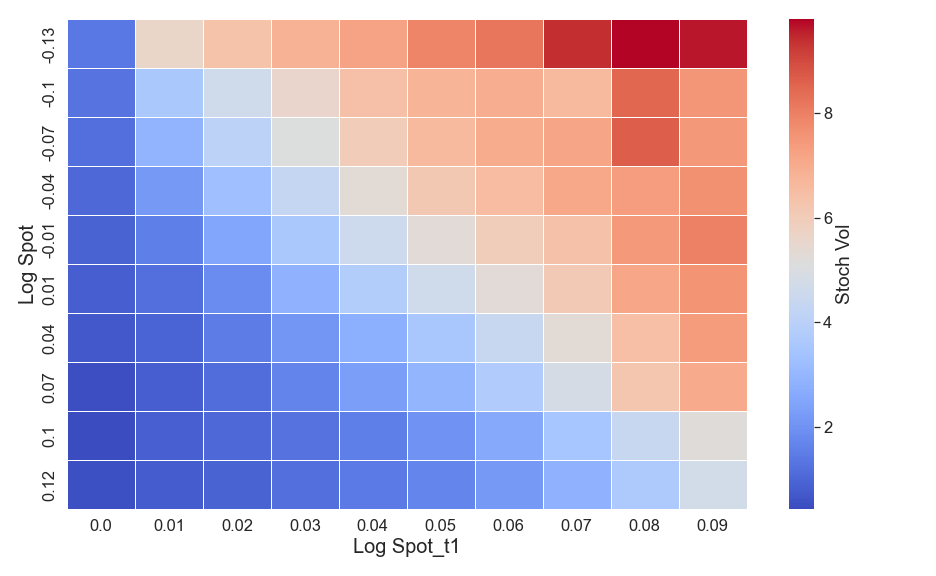
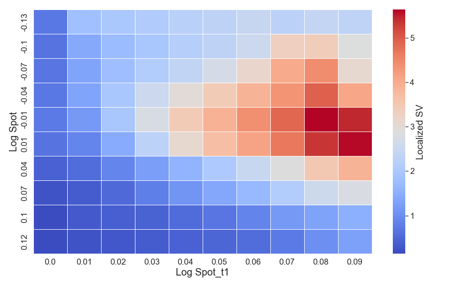
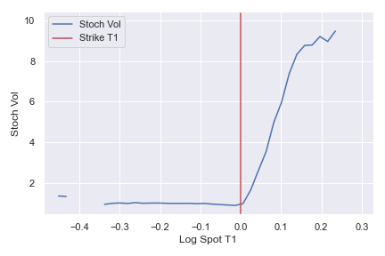
As an example, let us consider the case where consists of two types of options: european call options for all strikes (smile) and all dates , and a Bermudan option with exercise dates , , for which we have , where , are fixed and denotes the expectation conditional on , the information available up to . Due to and the "" non-linearity, the Bermudan option price depends on the forward smile and cannot be replicated with vanillas. Such option price is lower bounded by the maximum of the two european call options , , which we call maximum european: 111remember that .. Assume that is close to its lower bound, so that our goal is to find so as to minimize . First, notice that equals the maximum european means that if the maximum european is on , we should never exercise at for any path , and vice-versa if the maximum european is on . One can make the following heuristic reasoning to get the intuition that for must remember the value of , and hence be path-dependent, if we hope to minimize . If the maximum european is on , you need on paths for which is high, a high volatility on so that you do not exercise at . If the maximum european is on , the conclusion is the same, although the reasoning is different: you need to allocate high volatility on paths where is high, since doing so on paths where it is low will clearly result in not exercising at . Note that we use the terminology "allocate volatility", since the (unconditional) aggregated variances and are fixed by vanilla market smiles. Our informal reasoning will be validated by our learnt in figures 3-4.
It has been shown in Guyon, (2014) that volatility can, in theory, be path-dependent while preserving perfect fit to vanilla smiles. Even then, the difficulty lies in choosing the specific form of path dependence. Guyon provides examples of how to choose it in a heuristic way so as to achieve specific features, for example on the forward smile. The now popular class of rough volatility models Gatheral et al., (2018) also falls into the path-dependent category. The novel work of Cuchiero et al., (2020); Gierjatowicz et al., (2020) let be a neural network and calibration is performed via deep learning. Among other things, this opens the door to learning complex path-dependence of the volatility process, even though this aspect is not explored in these works. In particular, this approach requires storing the whole computational graph, which, due to memory considerations, limits the number of time steps and Monte Carlo trajectories that one can use to simulate the diffusion process. For this reason, both these work consider a small number of maturities to be calibrated (4-6), one neural network per maturity, and train one maturity at a time, since "training all neural networks at every maturity all at once, makes every step of the gradient algorithm used for training computationally heavy". Note that the same limitation has been identified in the learning to optimize literature, where the goal is to replace the traditional optimization gradient step by a neural network Chen et al., (2020, 2021). There, because of the aforementioned memory bottleneck, one typically trains on short time horizons, or optimization trajectories.
Contribution. We introduce a novel game theoretical formulation of the calibration problem 1 where individual particles acting locally cooperate towards the calibration objective at aggregate level. We introduce a numerical method to solve it by leveraging existing developments in modern deep multi-agent reinforcement learning to search in the space of stochastic processes. The latter is a reinforcement learning driven alternative to the aforementioned deep learning based approaches, which in particular doesn’t require storing the computational graph and as such doesn’t suffer from memory bottlenecks. This allows us to "train" all maturities at once using the concept of rewards obtained along agent trajectories, which is required in particular to handle the Bermudan option case discussed above, or to calibrate to a continuum of vanilla smiles in one shot, as we do in our experiments. In essence, our idea is to see Monte Carlo trajectories as players participating in a cooperative game, where player ’s action at time is the choice of the volatility to be used on trajectory over , and where the common reward that players try to minimize is the calibration error, which is, in game theoretical terms, a function of all players’ individual actions. Our experiments show that we are able to learn local volatility, as well as the path-dependence required to minimize the price of the Bermudan option previously discussed, matching our initial intuition. Finally, on the multi-agent reinforcement learning side, we introduce a new technique to handle the case of a very large number of players (), that turned out to be crucial in making our method work, where policy exploration across all players is obtained via interpolation of a few basis players ().
2 Game theoretical formulation of the calibration problem
As stated in introduction, we let be the stochastic price path process over some finite time horizon on a complete probability space and consider continuous-time diffusion models of the form:
| (1) |
where is a Brownian motion and is allowed to be a very general stochastic process.
We start by giving a concise exposition of the key concepts in Markov decision processes (single-agent case) and stochastic games (multi-agent case), that we will use to develop our approach. Reinforcement learning (RL) and its multi-agent counterpart (MARL) are used as numerical methods to solve the latter, which we will focus on in section 3. We refer to Sutton and Barto, (2018) for a presentation of the core concepts in RL, and Jaimungal, (2022); Hambly et al., (2021) illustrate some of its applications to finance.
Under a Markov decision process framework, an agent evolves over a series of discrete time steps . At each , it observes some information called its "state" , takes an action , and as a consequence, transitions to a new state as well as gets a reward , where the transition dynamics is called the "environment" and denotes the probability to reach conditional on . The design of the state is quite flexible, in particular one can include time as well as path-dependent information. This is even more true since the recent developments around neural networks which can be fed a large amount of information, and aforementioned path-dependent data can be encoded by means of the hidden state of a LSTM (long short-term memory). The agent samples its actions according to the stochastic policy representing the probability density function of conditionally on , and its goal is simply to maximize its expected cumulative reward:
| (2) |
where indicates that , and is usually called the value function. We focus here on the finite time horizon case and omit the classical discounting of rewards by since we do not need it in the present work. Due to the finite time horizon, we assume that includes time , since it is well-known that solutions of (2) must be time-dependent. A stochastic game is simply the extension of a Markov decision process to players: each agent is now allowed to have its own policy and reward function , but the latter now depends, in the most general case, on all agents’ actions and states , where we denote vectors in bold , . We consider the fully observable case where each player observes information and actions from all players at each time . We focus our attention on symmetric cooperative games where:
-
•
(cooperation) all agents rewards are the same .
-
•
(symmetry) agents are interchangeable: for all permutations , where the "superscript " denotes the permuted vector. In simple terms, this condition means that what matters is "what" is done and "where", but not "who" did it. In mathematical terms, the "what", "where" and "who" are respectively , , and .
One should think about such games as a set of interacting particles, or ants, acting locally towards a common goal at the aggregate level.
Solving cooperative games in the context of MARL has for example been studied in Gupta et al., (2017); Foerster et al., (2016). Similar to the single-agent case (2), we denote the value function of the symmetric cooperative game:
| (3) |
Definition 1.
(Nash equilibrium) The vector of players’ policies of the symmetric cooperative game associated to value function in (3) is a Nash equilibrium if:
| (4) |
where denotes the value of the game associated to , but with replaced by .
In simple terms, no player has an incentive to deviate unilaterally in a Nash equilibrium.
Back to our calibration problem. Let each Monte Carlo trajectory be a player, so that is the number of Monte Carlo trajectories, typically very large (). Let player ’s action , the volatility to use for trajectory over the timestep . We can more generally allow for some distribution , but we discuss this later. The discretization of the dynamics (1) yields:
| (5) |
where is a collection of i.i.d. standard normal random variables and is the time step value, for example for a time step of one day. The state typically contains spot and volatility for trajectory over a past historical window of size , , as well as time . It could also contain information relative to other trajectories, to include the McKean-Vlasov case where the diffusion coefficients depend on . As previously mentioned, the now standard technique to encode history of observations, required for example in imperfect information games, is via the hidden state of a LSTM Gupta et al., (2017), but other approaches are possible, for example path signatures Arribas et al., (2020).
We assume that we have option cashflows associated to market target prices . Option cashflows are random variables, and each is assumed to be a function of , remembering from our previous discussion that states can potentially encapsulate a large amount of information, including path-dependent one. We then define the game reward obtained at as the calibration loss:
| (6) | ||||
where are weights chosen by the user (for example related to the Vega of the option), is the Monte Carlo price and a suitable transformation, for instance the Black & Scholes implied volatility mapping in the case of a call option, in which case would be the market implied volatility. In the case of a call option, we have . In the case of the Bermudan, we have for and , where the conditional expectation is calculated empirically using all trajectories over using, for instance, American Monte Carlo regression methods Longstaff and Schwartz, (2001).
The deep MARL methods we employ in section 3 allow to have sparse reward signals as it is the case for the Bermudan option, the key being to use a neural network to approximate the value function, i.e. the expected sum of future rewards, given a particular state . Such approximation is called a "critic" in RL jargon, and was one of the keys to the success of AlphaGo, Deepmind’s pioneering work on the game of Go Silver et al., (2016).
Even though the true rewards can be sparse like in the Bermudan example, it is actually possible in many cases to construct per-timestep approximations of true rewards. Reward design, or "shaping" is an active area of research in RL. It consists in suitably designing the reward function to improve learning. In our case, it is perfectly reasonable to define "fake" cashflows and rewards such that cumulative rewards agree:
| (7) |
In the Bermudan example, a reasonable choice would be , where can be expressed either in percentage of the forward at time , or in delta space . We then define the fake rewards as:
| (8) |
where is the reward in (6) but associated to cashfows , and the implied volatility mapping associated to . One can observe that (7) is true due to the telescopic property (8) and that both and coincide at time .
In order to get a more meaningful reward signal, one should subtract to the reward in (6) the calibration error obtained with a reference model, for example the Black & Scholes model or the local volatility model.
We have the following game theoretical interpretation of the calibration problem, which follows by definition of the game reward (3), (6).
Proposition 2.1.
(Calibration as a Nash equilibrium) Let the number of Monte Carlo paths and time discretization value be fixed. Let be a minimizer, over all models simulated with Monte Carlo parameters , of the calibration error associated to a given set of options. Then is a Nash equilibrium of the calibration game.
Our calibration game is symmetric, so it is common to look for symmetric equilibria, i.e. where all players play the same strategy Vadori et al., (2020); Li and Wellman, (2021); Hefti, (2017). Asymmetric equilibria of symmetric games exist but they represent a degenerate case Fey, (2012), i.e. they are not natural and one has to work hard to identify them. We discuss in section 3 MARL driven methods to find such equilibria.
Players’s actions and volatility dynamics . For simplicity, we previously defined the volatility to be players’ actions: . Note that since actions are sampled from the distribution , they are by construction stochastic. It is however straightforward to consider a distribution parametrized by (a vector of) parameters , and simply define players’ actions to be those parameters, i.e. . Specific examples of such include the case where are parameters of a Gaussian mixture, possibly correlated with . In that case the overall correlation matrix is of size (volatility and spot), where is the number of components in the mixture. The rationale for adding more components is to make volatility increments deviate from Gaussianity, conditional on . In particular, this includes the case where are parameters driving the SDE of , where are independent from as in (5):
| (9) |
It is important to keep in mind that since actions depend on the state , which as discussed can encapsulate complex information such as path-dependence, can be complex functions of the state.
3 Multi-agent reinforcement learning of the calibration game
We discuss in this section a MARL-based method to solve empirically the game presented in section 2. Our main innovation is the concept of basis players needed to handle large number of players , which turned out to be crucial in making our algorithm work. We postpone to future work the connection of our algorithm to mean-field RL based methods. We will consider a policy gradient approach, i.e. where is a neural network with parameters that will be iteratively improved.
Our action and state spaces are continuous as subsets of , and we aim at finding symmetric equilibria of the symmetric game, as discussed in section 2, i.e. one where all players play the same strategy. Denoting the expected utility of player when it plays while all others play , one can find symmetric equilibria by solving:
| (10) |
This was done in Li and Wellman, (2021) and takes its origins in Hefti, (2017) under the name SOFA (symmetric opponents form approach). In our context, the and operations each involve solving a RL problem, so they are costly. The alternative that we will adopt is to approximate by a gradient step. This is a form of self-play, but in the context of players, where players, the "rest of the world", are tied together by a policy . This was discussed in Vadori et al., (2020, 2023) under the name shared equilibrium, where it was shown that policy sharing among players amounts to picking one player at random and making a step towards improving its reward, while freezing other players. In general, it is important to understand that convergence of self-play is linked to transitivity in games and is different, for example, from maximizing the sum of players’ rewards. As a simple example, the game where 2 players receive respectively and has by construction a sum of players’ utilities equal to zero, but optimizing at each training iteration the utility of a randomly selected player will eventually lead to finding a (local) maximizer of .
Recent successes of policy gradient methods are based on two pillars: the policy network , and the value function network , parametrized by . estimates the expected sum of future rewards of an agent currently in state and serves as a variance reduction method. The advantage represents the benefit of action in state , relative to some average level in state :
| (11) | ||||
The conditional expectation appearing in is estimated by a sample of the simulated trajectory, but it could be estimated using truncated trajectories instead (Generalized Advantage Estimation) Schulman et al., (2016).
The gradient according to which the shared policy is updated is computed by collecting all players’ experiences simultaneously and treating them as distinct sequences of local states, actions and rewards experienced by the shared policy Gupta et al., (2017); Vadori et al., (2020), yielding the following expression under A2C (advantage actor critic) Mnih et al., (2016), where we allow a set of parallel runs :
| (12) |
The gradient in equation (12) is presented in the context of A2C, but other policy gradient updates based on and can be used instead, for example we use proximal policy optimization (PPO) in our experiments Schulman et al., (2017).
The value network is estimated classically by performing a few steps of mini-batch gradient descent on the following objective, at each policy update:
| (13) |
Basis players. The gradient update (12) scales with the time horizon and the number of players . It is clearly not efficient when is large. In the case of local volatility or particle methods Guyon and Henry-Labordere, (2012), one does not compute the leverage function at every timestep of every Monte Carlo path, as it would be highly inefficient. Instead, one computes it on a much smaller grid of size in space and interpolate. We take inspiration from this idea to interpolate all players from a smaller set of basis players. In practice, a common choice for the action space exploration strategy in policy gradient methods is to let output the mean and standard deviation of actions:
| (14) | ||||
and are natural interpolators, so and can simply be computed by the forward pass of a neural network and as such can be evaluated cheaply for all trajectories . The exploration variable represents how players explore the space of actions and find "good" and "bad" actions, by using (12) to update their knowledge. Without , i.e. , equation (12) would not lead to any policy improvement. It is the analogous of the exploration policy used in learning, typically -greedy. Our innovation is to compute action of each trajectory as:
| (15) | ||||
where is interpolated from the basis players’ exploration . This way, exploration performed by basis players is propagated to the whole Monte Carlo computation, as each basis player impacts other players in its neighborhood via interpolation. As an interpolation method, we tried linear interpolation and -nearest neighbors (-NN), and both yielded similar results 222LinearNDInterpolator and KNeighborsRegressor in SciPy.. Basis players are picked at random among the trajectories at every time . We summarize our approach in algorithm 1.
Input: learning rate , initial policy and value network parameters , , number of basis players .
4 Experiments
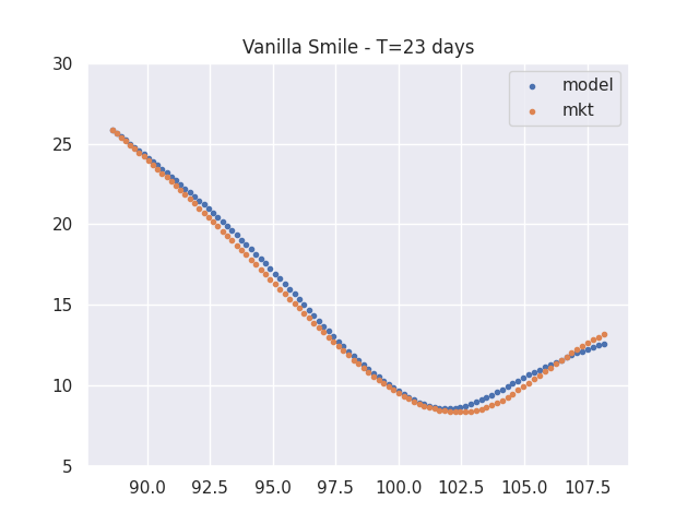
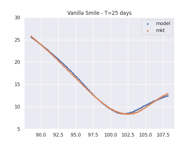
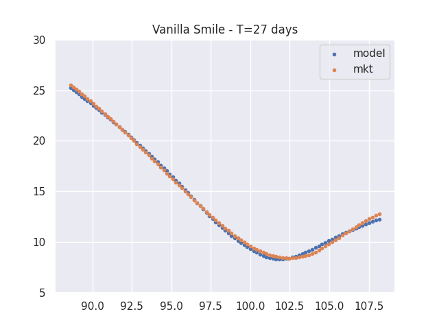
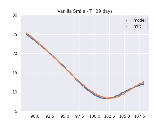
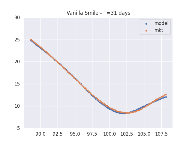
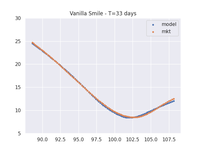
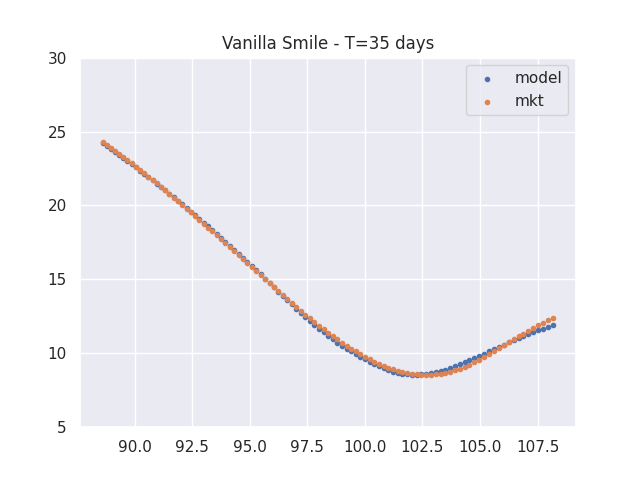
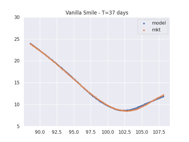
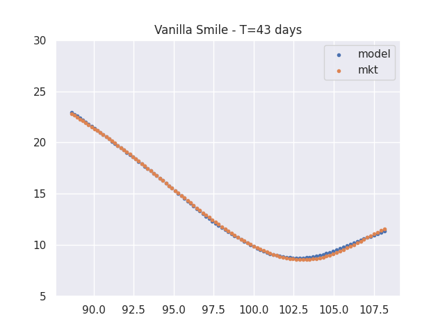
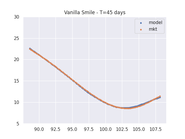
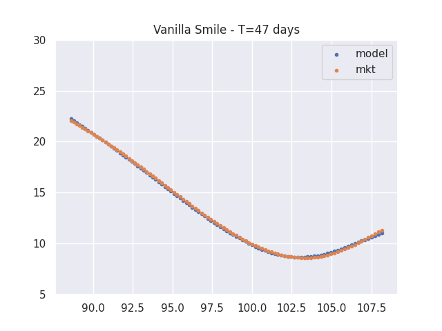
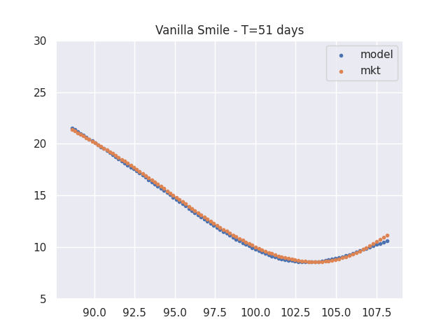
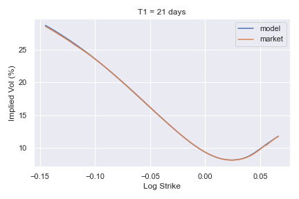
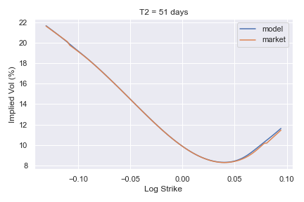
We consider S&P 500 (SPX) smiles as of August 1st 2018 for days and days. Smiles for dates in between are interpolated.
We first learn local volatility: our target instruments are all call options for all maturities up to . We see in figure 1 that we are able to fit the continuum of market smiles. In this case consists of , and actions consist of the mean and variance of a normal distribution, which we sample from. We trained using a time step day (), so that , trajectories, parallel runs and basis players. We checked empirically that the results are not too sensitive to these parameters, for example we considered ( day), , and from 20 to 100. Our approach doesn’t suffer too much from increasing these parameters except from the incompressible cost of the Monte Carlo simulation, since we do not need to store the computational graph as discussed in section 1.
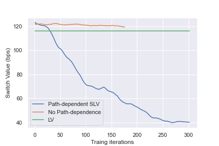
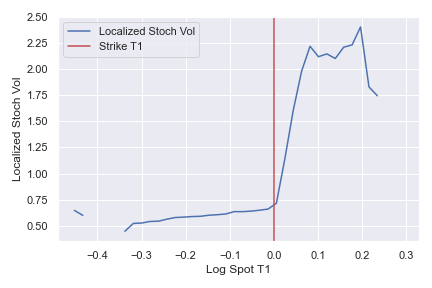
We then turn to the Bermudan case for which we have . We choose strikes , , so that the vanilla calls , have the same value: this is the interesting case, since if one call is worth much more than the other, the Bermudan price will already be close to its maximum european lower bound. We define the switch value as the difference between the Bermudan and the maximum european prices, both expressed in implied volatility points associated to . By construction the switch value is nonnegative. We consider similar numerical parameters as in the local volatility case, and considered different ways to define actions as discussed in section 2 and in (9), but our conclusions remained similar. The option price is calculated using American Monte Carlo Longstaff and Schwartz, (2001) with polynomial regression of degree 8. We compare two cases regarding the construction of (i) the path-dependent case considers , and (ii) the non path-dependent case considers . We see in figure 2 that path-dependence is required to minimize the price, while remaining calibrated to vanillas. Note that in this case, our calibration reward only consists of the Bermudan objective, while we ensure calibration to vanillas for all dates using localization. We check in figures 3-4 the nature of the learnt path-dependence, and we see that as intuited in section 1, we learn a volatility increasing in , decreasing in . In figure 4, we see that the cutoff strike is perfectly learnt by our RL policy, as it is obviously never optimal to exercise at if .
Due to the flexibility in defining the state , our approach can be extended straightforwardly to more Bermudan dates, where path-dependent information corresponding to past exercise dates is fed into the state process.
The RL policy was trained in the RLlib framework Liang et al., (2018), and run on AWS using a EC2 C5 4xlarge instance with CPUs, using Proximal Policy Optimization Schulman et al., (2017). We used configuration parameters in line with the latter paper, that is a clip parameter of 0.3, an adaptive KL penalty with a KL target of and a learning rate of . Each policy update was performed with 30 iterations of stochastic gradient descent with SGD minibatch size of . We used a fully connected neural net with 3 hidden layers, 50 nodes per layer, and activation. Although is much more expensive to evaluate than ReLU, we noticed that it lead to smoother and more efficient learning.
5 Conclusion
In this paper we provided a novel view on the derivative pricing model calibration problem using game theory and multi-agent reinforcement learning. We illustrated its ability to learn local volatility, as well as path-dependence in the volatility process required to minimize Bermudan option prices.


Disclaimer
This paper was prepared for information purposes by the Artificial Intelligence Research group of JPMorgan Chase & Co and its affiliates (“JP Morgan”), and is not a product of the Research Department of JP Morgan. JP Morgan makes no representation and warranty whatsoever and disclaims all liability, for the completeness, accuracy or reliability of the information contained herein. This document is not intended as investment research or investment advice, or a recommendation, offer or solicitation for the purchase or sale of any security, financial instrument, financial product or service, or to be used in any way for evaluating the merits of participating in any transaction, and shall not constitute a solicitation under any jurisdiction or to any person, if such solicitation under such jurisdiction or to such person would be unlawful.
References
- Arribas et al., (2020) Arribas, I. P., Salvi, C., and Szpruch, L. (2020). Sig-SDEs model for quantitative finance. Proceedings of the First ACM International Conference on AI in Finance.
- Chen et al., (2021) Chen, T., Chen, X., Chen, W., Heaton, H., Liu, J., Wang, Z., and Yin, W. (2021). Learning to Optimize: A Primer and A Benchmark. https://arxiv.org/abs/2103.12828.
- Chen et al., (2020) Chen, T., Zhang, W., Zhou, J., Chang, S., Liu, S., Amini, L., and Wang, Z. (2020). Training Stronger Baselines for Learning to Optimize. NeurIPS.
- Cuchiero et al., (2020) Cuchiero, C., Khosrawi, W., and Teichmann, J. (2020). A generative adversarial network approach to calibration of local stochastic volatility models. Risks.
- Fey, (2012) Fey, M. (2012). Symmetric games with only asymmetric equilibria. Games and Economic Behavior, 75(1):424–427.
- Foerster et al., (2016) Foerster, J. N., Assael, Y. M., de Freitas, N., and Whiteson, S. (2016). Learning to communicate with deep multi-agent reinforcement learning. In Proceedings of the 30th International Conference on Neural Information Processing Systems, NIPS’16, page 2145–2153.
- Gatheral et al., (2018) Gatheral, J., Jaisson, T., and Rosenbaum, M. (2018). Volatility is rough. Quantitative Finance.
- Gierjatowicz et al., (2020) Gierjatowicz, P., Sabate-Vidales, M., Siska, D., Szpruch, L., and Zuric, Z. (2020). Robust pricing and hedging via neural SDEs. https://arxiv.org/abs/2007.04154.
- Gupta et al., (2017) Gupta, J. K., Egorov, M., and Kochenderfer, M. (2017). Cooperative multi-agent control using deep reinforcement learning. In Autonomous Agents and Multiagent Systems, pages 66–83. Springer International Publishing.
- Guyon, (2014) Guyon, J. (2014). Path-dependent volatility. Risk Magazine.
- Guyon and Henry-Labordere, (2012) Guyon, J. and Henry-Labordere, P. (2012). Being particular about calibration. Risk Magazine.
- Hambly et al., (2021) Hambly, B., Xu, R., and Yang, H. (2021). Recent Advances in Reinforcement Learning in Finance. https://arxiv.org/abs/2112.04553.
- Hefti, (2017) Hefti, A. (2017). Equilibria in symmetric games: Theory and applications. Theoretical Economics.
- Jaimungal, (2022) Jaimungal, S. (2022). Reinforcement learning and stochastic optimisation. Finance and Stochastics, 26:103–129.
- Li and Wellman, (2021) Li, Z. and Wellman, M. P. (2021). Evolution Strategies for Approximate Solution of Bayesian Games. Proceedings of the AAAI Conference on Artificial Intelligence.
- Liang et al., (2018) Liang, E., Liaw, R., Nishihara, R., Moritz, P., Fox, R., Goldberg, K., Gonzalez, J., Jordan, M., and Stoica, I. (2018). RLlib: Abstractions for distributed reinforcement learning. In Proceedings of the 35th International Conference on Machine Learning, volume 80 of Proceedings of Machine Learning Research, pages 3053–3062.
- Longstaff and Schwartz, (2001) Longstaff, F. A. and Schwartz, E. S. (2001). Valuing american options by simulation: A simple least-squares approach. The Review of Financial Studies., 14:113–147.
- Mnih et al., (2016) Mnih, V., Badia, A. P., Mirza, M., Graves, A., Harley, T., Lillicrap, T. P., Silver, D., and Kavukcuoglu, K. (2016). Asynchronous methods for deep reinforcement learning. In Proceedings of the 33rd International Conference on International Conference on Machine Learning - Volume 48, ICML’16, page 1928–1937. JMLR.org.
- Schulman et al., (2016) Schulman, J., Moritz, P., Levine, S., Jordan, M., and Abbeel, P. (2016). High-Dimensional Continuous Control Using Generalized Advantage Estimation. ICLR.
- Schulman et al., (2017) Schulman, J., Wolski, F., Dhariwal, P., Radford, A., and Klimov, O. (2017). Proximal Policy Optimization Algorithms. https://arxiv.org/abs/1707.06347.
- Silver et al., (2016) Silver, D., Huang, A., Maddison, C. J., Guez, A., Sifre, L., van den Driessche, G., Schrittwieser, J., Antonoglou, I., Panneershelvam, V., Lanctot, M., Dieleman, S., Grewe, D., Nham, J., Kalchbrenner, N., Sutskever, I., Lillicrap, T., Leach, M., Kavukcuoglu, K., Graepel, T., and Hassabis, D. (2016). Mastering the game of Go with deep neural networks and tree search. Nature, 529(7587):484–489.
- Sutton and Barto, (2018) Sutton, R. S. and Barto, A. G. (2018). Reinforcement Learning: An Introduction. The MIT Press, second edition.
- Vadori et al., (2023) Vadori, N., Ardon, L., Ganesh, S., Spooner, T., Amrouni, S., Vann, J., Xu, M., Zheng, Z., Balch, T., and Veloso, M. (2023). Towards multi-agent reinforcement learning driven over-the-counter market simulations. Mathematical Finance, Special Issue on Machine Learning in Finance.
- Vadori et al., (2020) Vadori, N., Ganesh, S., Reddy, P., and Veloso, M. (2020). Calibration of Shared Equilibria in General Sum Partially Observable Markov Games. Advances in Neural Information Processing Systems (NeurIPS).