A Single Correspondence Is Enough: Robust Global Registration
to Avoid Degeneracy in Urban Environments

Abstract

Global registration using 3D point clouds is a crucial technology for mobile platforms to achieve localization or manage loop-closing situations. In recent years, numerous researchers have proposed global registration methods to address a large number of outlier correspondences. Unfortunately, the degeneracy problem, which represents the phenomenon in which the number of estimated inliers becomes lower than three, is still potentially inevitable. To tackle the problem, a degeneracy-robust decoupling-based global registration method is proposed, called Quatro. In particular, our method employs quasi-SO(3) estimation by leveraging the Atlanta world assumption in urban environments to avoid degeneracy in rotation estimation. Thus, the minimum degree of freedom (DoF) of our method is reduced from three to one. As verified in indoor and outdoor 3D LiDAR datasets, our proposed method yields robust global registration performance compared with other global registration methods, even for distant point cloud pairs. Furthermore, the experimental results confirm the applicability of our method as a coarse alignment. Our code is available: https://github.com/url-kaist/quatro

I Introduction

3D point cloud registration is a method to align 3D point clouds by estimating relative pose or poses between two or more 3D point clouds [1]. 3D registration methods are widely utilized in various research fields such as object recognition [2, 3, 4, 5], mapping [6, 7, 8], localization [9, 10, 11, 12], and so forth. In particular, 3D registration is also a fundamental task for terrestrial mobile platforms to estimate ego-motion [13, 14], i.e. odometry, and to manage loop closing situations [15, 16].

Accordingly, the registration algorithms are mainly divided into two categories. One is the local registration [17, 18, 19, 20, 21, 22], and the other is the global registration [23, 24, 25, 26, 27]. Iterative Closest Point (ICP) [17] is a renowned local registration method and it has made an impact on subsequent studies. Unfortunately, the ICP-variants set point pairs by using a greedy, exhaustive nearest neighbor (NN) search for every iteration. Consequently, the local registration methods are only applicable when two point clouds, namely source and target, are close enough and nearly overlapped [22]. Otherwise, the correspondences via the NN search are likely to become invalid; thus, the result of the local registration may get caught in the local minima [20].

The global registration [23, 24, 25, 26, 27], on which this paper places emphasis, aims to estimate the relative pose between distant and partially overlapped point clouds. Because the global registration is relatively invariant to the initial pose difference, the global registration is usually used to provide an initial alignment close enough for the local registration to allow the estimate to converge on the global minima. The global registration can be further classified into correspondence-based [23, 26, 27, 28] and correspondence-free methods [29, 30, 31], but the latter ones are beyond our scope.

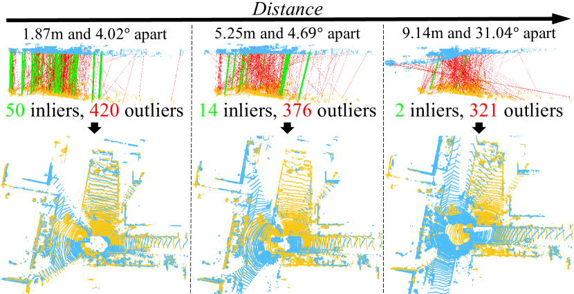
Figure 1: (T-B, L-R): Before and after the application of our proposed method called Quatro in KITTI dataset [7] when two distant and partially overlapped point clouds, i.e. source (cyan) and target (yellow), are given. As the distance between the two viewpoints of source and target becomes farther, it gives rise to an increase in the ratio of outliers within the putative correspondences and simultaneously reduces the number of inliers, which results in the performance degradation of correspondence-based global registration methods in general [23, 26, 28]. Under the circumstances, our proposed method shows robust performance, overcoming the effect of outliers, as well as the degeneracy issue. The red and green lines denote outlier and inlier correspondences, respectively (best viewed in color).

Some of the well-known correspondence-based methods are random sample consensus (RANSAC) [23] and its variants [32, 33, 34, 35], yet these are known to become slow and brittle with high outlier rates ($>50$%) [28]. On the other hand, branch-and-bound (BnB)-based methods [36, 37, 38] have been proposed for theoretical optimality guarantees. Unfortunately, BnB-based methods are not applicable to real-world applications because they are time-consuming ($>50$ sec) [39].

Aiming for both outlier-robust and fast registrations, graduated non-convexity (GNC) has been introduced based on Black-Rangarajan duality [40, 26]. For instance, Zhou et al. [26] showed that GNC outperforms previous approaches and is faster than existing methods by at least ten times, while tolerating 70-80% of outliers. As a result, many researchers have employed GNC to achieve robust pose estimation [28, 27, 41, 42]. In the meantime, semidefinite programming and sums of squares relaxation-based methods have been proposed to solve problems in polynomial-time with certifiable optimality guarantees [43, 44, 45, 46]. Further, novel graph-theoretic methods also have been proposed to prune spurious correspondences effectively [47, 48].

Unfortunately, a degeneracy problem is still potentially inevitable. Degeneracy usually refers to various phenomena in the perceptually degraded environments, such as corridors, mines, and so forth [49, 50, 51]. However, in this paper, we specify degeneracy as the phenomenon in which the number of the estimated inliers becomes lower than the minimum number of inliers during registration, which is generally three in the 3D space. Note that this effect can occur not only in the perceptually degraded environments but also in some cases where two distant and partially overlapped point clouds are given, resulting in catastrophic failure of global registration.

To sum up, the reason for the degeneracy problem is mainly twofold. First, there is a sparsity issue with 3D LiDAR sensors [52, 53, 54, 55], which means, as the distance from the sensor coordinate becomes farther away, a point cloud becomes too sparse; thus, it induces inaccurate feature matching. That is, even though the two point clouds represent the same space locally, the local areas have different densities because the source and target are captured in a different location. Consequently, the sparsity issue directly affects the quality of feature descriptors and then gives rise to more false correspondences. Thus, the ratio of the outliers within the putative correspondences increases, as shown in Fig. 1. Second, these outlier pairs let the outlier-rejection algorithms, such as graph-theoretic pruning methods [47, 48] or weight update in GNC [26, 27], reject the putative correspondences dramatically to prune outliers. Accordingly, too many correspondences are occasionally filtered. Finally, the number of the estimated inliers occasionally becomes less than three in the process, resulting in degeneracy.

To tackle the degeneracy problem, we propose a novel global registration method, called Quatro, which is a combination of the words Quasi- and cuatro meaning 4-DoF (degree of freedom). Some degeneracy-aware SLAM frameworks have been proposed in [49, 50, 51]. However, to the best of our knowledge, this is the first attempt to deal with the degeneracy in global registration by reducing the minimum number of required correspondences of SE(3) from three to one, named quasi-SE(3) by decoupling SE(3) estimation into quasi-SO(3) estimation followed by component-wise translation estimation (COTE) [27].

In summary, the contribution of this paper is threefold.

• To avoid degeneracy, we propose a novel rotation estimation method called quasi-SO(3) estimation by utilizing the characteristics of urban environments.

• As a result, our proposed method shows a more promising performance over the state-of-the-art methods on real-world indoor/outdoor 3D LiDAR datasets.

• In particular, it is remarkable that Quatro-c2f, a simple coarse-to-fine scheme, outperforms the state-of-the-art methods, including deep learning-based approaches. Therefore, we finally confirm the suitability of our proposed method as a coarse alignment.

II Quatro: Quasi-SE(3) Estimation

II-A Problem Definition

First, we begin by denoting source and target point cloud which are captured by a 3D LiDAR sensor on different viewpoints as $\mathcal{P}$ and $\mathcal{Q}$, respectively. Then, let us define $\mathcal{P}=\{\mathbf{p}_{1},\mathbf{p}_{2},\dots,\mathbf{p}_{N}\}$ and $\mathcal{Q}=\{\mathbf{q}_{1},\mathbf{q}_{2},\dots,\mathbf{q}_{M}\}$, where each point of the clouds, $\mathbf{p}_{i}\leavevmode\nobreak\ (1\leq i\leq N)$ and $\mathbf{q}_{j}\leavevmode\nobreak\ {(1\leq j\leq M)}$ $\in\mathbb{R}^{3}$, consists of $\{x,y,z\}$ in the Cartesian coordinate. It is assumed that the $xy$-plane of $\mathcal{P}$ and $\mathcal{Q}$ are already aligned with that of mobile platforms to utilize the Atlanta world assumption [56] (see Section II.C).

Next, let $(i,j)\in\mathcal{A}$ be candidate correspondences where $i$ and $j$ denote the indices of points in $\mathcal{P}$ and $\mathcal{Q}$, respectively. In practice, $\mathcal{A}$ inevitably includes inherent outlier set $\mathcal{O}$, such that $\mathcal{O}\cup\mathcal{O}^{c}=\mathcal{A}$. This happens in most of the 3D point feature matching algorithms [28, 57, 58]. Accordingly, the relationship of each pair can be expressed as follows:

$$\mathbf{q}_{j}=\mathbf{R}\mathbf{p}_{i}+\mathbf{t}+\boldsymbol{\epsilon}_{ij}$$ (1)

where $\mathbf{R}\in\mathrm{SO}(3)$ and $\mathbf{t}\in\mathbb{R}^{3}$ are the relative rotation and translation, respectively, and $\boldsymbol{\epsilon}_{ij}\in\mathbb{R}^{3}$ denotes the unknown measurement noise. That is, $\boldsymbol{\epsilon}_{ij}$ is Gaussian noise if $(i,j)\leavevmode\nobreak\ \in\leavevmode\nobreak\ \mathcal{O}^{c}$ or is irregular error if $(i,j)\leavevmode\nobreak\ \in\leavevmode\nobreak\ \mathcal{O}$. Finally, our objective function could be defined as follows:

$$\hat{\mathbf{R}},\hat{\mathbf{t}}=\mathop{\mathrm{argmin}}_{\mathbf{R}\in\mathrm{SO}(3),\mathbf{t}\in\mathbb{R}^{3}}\sum_{(i,j)\in\mathcal{A}}\rho\Big{(}r(\mathbf{q}_{j}-\mathbf{R}\mathbf{p}_{i}-\mathbf{t})\Big{)}$$ (2)

where $\rho(\cdot)$ denotes surrogate function [28] to suppress undesirable large errors produced by $\mathcal{O}$ and $r(\cdot)$ denotes the squared residual function, i.e. $\absolutevalue{\cdot}^{2}$. In summary, our goal is to estimate $\hat{\mathbf{R}}$ and $\hat{\mathbf{t}}$ while suppressing the effect of outliers as much as possible by employing $\rho(\cdot)$.

II-B Decoupling Rotation and Translation Estimation

According to [59] and [60], $\hat{\mathbf{R}}$ and $\hat{\mathbf{t}}$ can be easily obtained in closed form by decoupling rotation and translation estimation. To this end, first of all, two pairs ($i$, $j$) and ($i^{\prime}$, $j^{\prime}$) are subtracted to cancel out the effect of $\mathbf{t}$ by using (1). For simplicity, let $\boldsymbol{\alpha}_{k}\leavevmode\nobreak\ =\leavevmode\nobreak\ \mathbf{p}_{i^{\prime}}-\mathbf{p}_{i}$; $\boldsymbol{\beta}_{k}\leavevmode\nobreak\ =\leavevmode\nobreak\ \mathbf{q}_{j^{\prime}}-\mathbf{q}_{j}$; $\boldsymbol{\epsilon}_{k}\leavevmode\nobreak\ =\leavevmode\nobreak\ \boldsymbol{\epsilon}_{i^{\prime}j^{\prime}}-\boldsymbol{\epsilon}_{ij}$, and let $K$ be the total number of these translation invariant measurements (TIMs) [27]. Note that $K=\absolutevalue{\mathcal{A}}$ by subtracting consecutive pairs to build TIMs in a chain form to minimize computational cost and the first TIM is made by the subtraction between the first and $\absolutevalue{\mathcal{A}}$-th pair.

Then, the relationship between $\boldsymbol{\alpha}_{k}$ and $\boldsymbol{\beta}_{k}$ can be expressed as $\boldsymbol{\beta}_{k}=\mathbf{R}\boldsymbol{\alpha}_{k}+\boldsymbol{\epsilon}_{k}$. Accordingly, $\hat{\mathbf{R}}$ is estimated as follows:

$$\hat{\mathbf{R}}=\underset{\mathbf{R}\in\mathrm{SO}(3)}{\mathop{\mathrm{argmin}}}\sum_{k=1}^{K}\min\Big{(}w_{k}r({\boldsymbol{\beta}}_{k}-\mathbf{R}{\boldsymbol{\alpha}}_{k}),\bar{c}^{2}\Big{)}$$ (3)

where $w_{k}$ denotes the weight of each pair and $\bar{c}$ denotes the truncation parameter to suppress the effect of potential outliers. This is followed by COTE [27] to calculate $\hat{\mathbf{t}}$ in an element-wise way as follows:

$${}^{l}{\hat{\mathbf{t}}}=\underset{{}^{l}\mathbf{t}\in\mathbb{R}}{\mathop{\mathrm{argmin}}}\sum_{(i,j)\in\mathcal{A}}^{\absolutevalue{\mathcal{A}}}\min\bigg{(}\frac{r({{}^{l}\mathbf{t}}-{{}^{l}\mathbf{v}_{ij}})}{\sigma_{ij}^{2}},{\bar{c}^{2}}\bigg{)}$$ (4)

where $\mathbf{v}_{ij}=\mathbf{q}_{j}-{\hat{\mathbf{R}}}\mathbf{p}_{i}$, $\sigma_{ij}$ is the noise bound, and ${}^{l}(\cdot)$ denotes the $l$-th element of a 3D vector, where $l=1,2,3$, i.e. $\hat{\mathbf{t}}=\{{{}^{1}\hat{\mathbf{t}}},{{}^{2}\hat{\mathbf{t}}},{{}^{3}\hat{\mathbf{t}}}\}$.

Thus, (2) is decomposed into (3) followed by (4) using $\hat{{\mathbf{R}}}$.

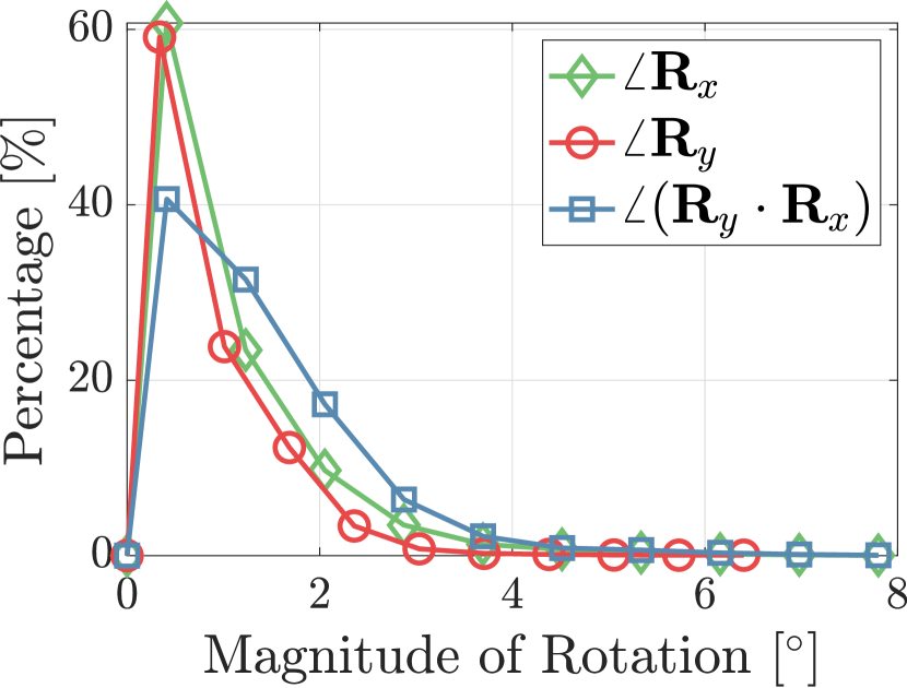
(a)

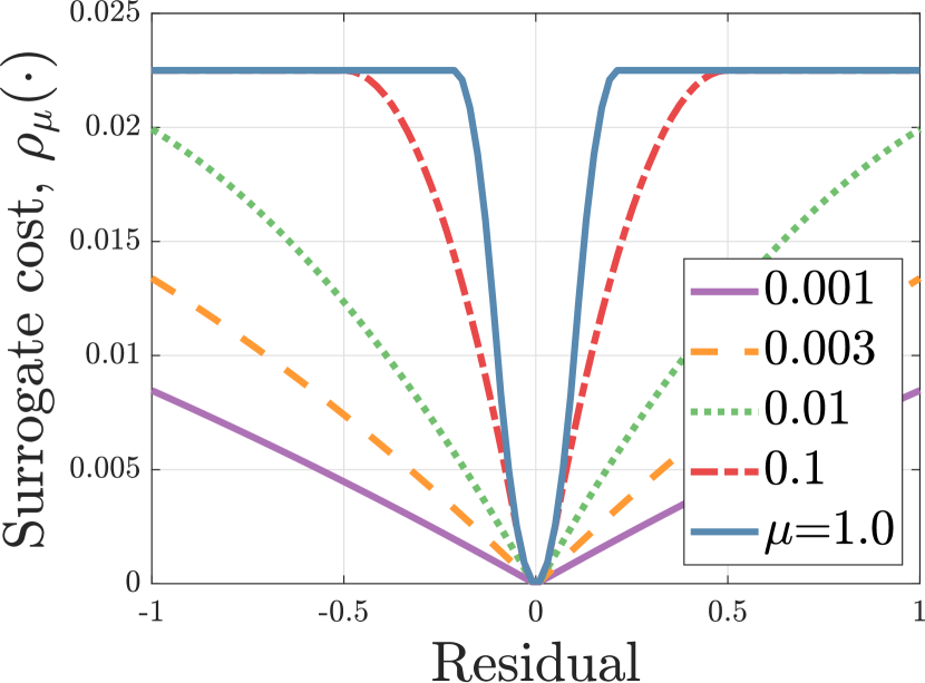
(b)

Figure 2: (a) Probability distribution function of the magnitudes of relative rotation between poses of source and target whose distances are between 0.5 to 10 m away in the KITTI dataset [7]. (b) Surrogate function $\rho_{\mu}(\cdot)$ that becomes convex if $\mu\rightarrow 0$ or truncated least squares if $\mu\rightarrow\infty$, where $\bar{c}=0.15$ (best viewed in color).

II-C Quasi-SO(3) in Urban Environments

Next, we introduce the concept of quasi-SO(3) to note that the relative rotation can be approximated as a pure yaw rotation in urban environments, which was postulated by Kim et al. [6] and Scaramuzza [61]. This is because, even though urban environments are not flat, two poses corresponding to the source and target cloud can be locally approximated to be coplanar based on the Atlanta world assumption [56]. Therefore, the yaw rotation is considered to be dominant than roll and pitch rotations.

To be more concrete, let us specify a relative rotation matrix $\mathbf{R}$ as $\mathbf{R}_{z}\cdot\mathbf{R}_{y}\cdot\mathbf{R}_{x}$, where $\mathbf{R}_{z}$, $\mathbf{R}_{y}$, and $\mathbf{R}_{x}$ denote rotation with respect to $z$, $y$, and $x$ axes, respectively. That is, these rotation elements denote yaw, pitch, and roll, respectively. As previously mentioned, the relative changes of pitch and roll were observed to be much smaller than that of yaw in urban canyons, i.e. $\angle\mathbf{R}_{z}\gg\angle(\mathbf{R}_{y}\cdot\mathbf{R}_{x})$, where $\angle\mathbf{R}=\cos^{-1}{\frac{\Tr(\mathbf{R})-1}{2}}$. In addition, as shown in Fig. 2(a), $\angle(\mathbf{R}_{y}\cdot\mathbf{R}_{x})$ is usually smaller than $10^{\circ}$; thus, the small angle assumption [62] is applicable, such that $\mathbf{R}_{y}\cdot\mathbf{R}_{x}\approx\mathbf{I}_{3}$, where $\mathbf{I}_{n}$ denotes an $n\times n$ identity matrix. This assumption results in $\mathbf{R}\approx\mathbf{R}_{z}$ and thus simplifies our goal to estimate $\mathbf{R}_{z}$ directly. Finally, this assumption reduces DoF of rotation from three to one, making our method robust against degeneracy. For simplicity, the approximated $\mathbf{R}$ is denoted by $\mathbf{R}_{+}$.

One might argue that this assumption does not hold in non-flat regions or if two viewpoints are no longer located in coplanar regions as the distance between two viewpoints increases [63, 64, 65]. However, most current mapping/navigation systems employ an inertial navigation system (INS). Accordingly, roll and pitch angles are fully observable by estimating the horizontal plane from the gravity vector [65, 66]. Consequently, the roll and pitch can be expressed as absolute states in the world coordinate, which means these are drift-free [67]. Thus, this still allows our goal to be valid, while restricting the relative rotation to relative yaw rotation (see Section IV.D).

II-D Quasi-SO(3) Estimation using Graduated Non-Convexity

To estimate $\mathbf{R}_{+}$, GNC with a truncated least square [28] is introduced. For simplicity, specifying the $k$-th measurement pair, i.e. $\boldsymbol{\alpha}_{k}$ and $\boldsymbol{\beta}_{k}$, as $\boldsymbol{\zeta}_{k}$, (3) can be redefined as $\mathop{\mathrm{argmin}}_{\mathbf{R}_{+}}\sum_{k=1}^{K}\rho_{\mu}\left(r\left(\boldsymbol{\zeta}_{k},\mathbf{R}_{+}\right)\right)$, where $\rho_{\mu}(\cdot)$ denotes surrogate function governed by parameter $\mu$, as shown in Fig. 2(b). For this, the equation is first rewritten by leveraging Black-Rangarajan duality as follows [26, 27]:

$$\hat{\mathbf{R}}_{+}=\mathop{\mathrm{argmin}}_{\mathbf{R}_{+}\in\mathrm{SO}(3),w_{k}\in[0,1]}\sum_{k=1}^{K}\left[w_{k}r\left(\boldsymbol{\zeta}_{k},\mathbf{R}_{+}\right)+\Phi_{\rho_{\mu}}\left(w_{k}\right)\right]$$ (5)

where $\Phi_{\rho_{\mu}}\left(w_{k}\right)=\frac{\mu\left(1-w_{k}\right)}{\mu+w_{k}}\bar{c}^{2}$ is a penalty term [42]. Unfortunately, the objective function cannot be directly solved [26]. Thus, (5) is solved by using alternating optimization as follows:

$$\hat{\mathbf{R}}^{(t)}_{+}=\underset{\mathbf{R}_{+}}{\mathop{\mathrm{argmin}}}\sum_{i=1}^{K}\hat{w}^{(t-1)}_{k}r\left(\boldsymbol{\zeta}_{k},\mathbf{R}_{+}\right),$$ (6)

$$\hat{\mathbf{W}}^{(t)}=\underset{w_{k}\in[0,1]}{\mathop{\mathrm{argmin}}}\sum_{k=1}^{K}\left[w_{k}r(\boldsymbol{\zeta}_{k},\hat{\mathbf{R}}^{(t)}_{+})+\Phi_{\rho_{\mu}}\left(w_{k}\right)\right]$$ (7)

where the superscript ^(t) denotes the $t$-th iteration and $\hat{\mathbf{W}}=\operatorname{diag}\left(\hat{w}_{1},\hat{w}_{2},\ldots,\hat{w}_{K}\right)$. Each $\hat{w}_{k}$ can be solved in a truncated closed form as follows:

$$\hat{w}_{k}^{(t)}=\begin{cases}0&\text{ if }\tilde{r}_{k}\in\left[\frac{\mu+1}{\mu}\bar{c}^{2},+\infty\right]\\ \bar{c}\sqrt{\frac{\mu(\mu+1)}{\tilde{r}_{k}}}-\mu&\text{ if }\tilde{r}_{k}\in\left[\frac{\mu}{\mu+1}\bar{c}^{2},\frac{\mu+1}{\mu}\bar{c}^{2}\right]\\ 1&\text{ if }\tilde{r}_{k}\in\left[0,\frac{\mu}{\mu+1}\bar{c}^{2}\right]\end{cases}$$ (8)

where $\tilde{r}_{k}$ denotes $r(\boldsymbol{\zeta}_{k},\mathbf{R}_{+}^{(t)})$ for simplicity. The overall procedure is illustrated in Fig. 3. For each iteration, $\mu$ is updated as $\mu^{(t)}\leftarrow\kappa\cdot\mu^{(t-1)}$, where $\mu^{(0)}={\bar{c}^{2}}/({\max(r(\boldsymbol{\zeta}_{k},\mathbf{I}_{3}))-\bar{c}^{2}})$ and $\kappa>1$ is a factor that increases the magnitude of non-convexity gradually, as presented in Fig. 2(b). The iteration ends if the differential of $\sum_{k=1}^{K}\hat{w}_{k}^{(t)}r(\boldsymbol{\zeta}_{k},\hat{\mathbf{R}}^{(t)}_{+})$ becomes small enough.

Figure 3: Illustration of Quatro in a degeneracy case when two distant and partially overlapped source (cyan) and target (yellow) are given. (a) Spurious correspondences. (b) The output of MCIS-heuristic. Most outliers are initially filtered. (c)-(e) An example of Quasi-SO(3) estimation via GNC. (c) First of all, all weights $w^{(0)}_{k}$ of TIMs are set to one. (d) During the optimization, sometimes GNC unexpectedly leaves less than three pairs by assigning near-zero values to some $w^{(t)}_{k}$ (red dashed rectangle). (e) In the degeneracy case, quasi-SO(3) estimation is successfully done because DoF of $\mathbf{R}_{+}$ is one, so it can be estimated even when a single pair of TIMs is left. (f) Before and the after the application of COTE. For (a), (b), and (f), the definite outliers, inliers, and quasi-inliers are represented by the red, green, and blue lines, respectively (best viewed in color).

Unfortunately, the outliers have a direct negative impact on the optimization at the first iteration because all the weights are initialized to 1, that is, $\hat{\mathbf{W}}^{(0)}=\mathbf{I}_{K}$ (Fig. 3(c)). Besides, in weight update, as in (8), most weights are occasionally assigned to zero (Fig. 3(d)), resulting in degeneracy in the 3D space (Figs. 3(d) and  3(g)). However, $\mathbf{R}_{+}$ is designed to suppress the effect of outliers, as well as to be robust against degeneracy; thus, catastrophic failure can be prevented, as shown in Fig. 3(e).

In short, $\mathbf{R}_{+}$ has advantages over $\mathbf{R}$ for the following three reasons. First, estimation of $\mathbf{R}_{+}$ resolves the degeneracy issue in itself. As previously mentioned, the number of estimated inliers is not always guaranteed to be more than the minimum DoF of rotation in GNC. However, note that the minimum DoF of $\mathbf{R}$ is three, whereas that of $\mathbf{R}_{+}$ is one. As a result, $\mathbf{R}_{+}$ can be more robust against degeneracy. Empirically, when the distance between the source and target viewpoints becomes more than 9 meters away, for example, in outdoor environments, the degeneracy occasionally occurs. However, our method can conduct robust registration, even if the two viewpoints are farther apart (see Section IV.A).

Second, $\mathbf{R}_{+}$ helps to suppress the effect of the outliers. Because the ground can be considered locally flat enough and most structures tend to be orthogonal to the ground, the local geometrical characteristics, e.g. surface normal, density, and so forth, are likely to be similar along the normal direction of the ground. Accordingly, the $\boldsymbol{\epsilon}_{k}$ can be decomposed into two terms: a) a parallel term to the ground plane, i.e. $xy$-plane, $\boldsymbol{\epsilon}^{||}_{k}$ and b) a perpendicular one $\boldsymbol{\epsilon}^{\perp}_{k}$, which satisfies $\boldsymbol{\epsilon}_{k}\leavevmode\nobreak\ =\leavevmode\nobreak\ \boldsymbol{\epsilon}^{||}_{k}\leavevmode\nobreak\ +\leavevmode\nobreak\ \boldsymbol{\epsilon}^{\perp}_{k}$. Consequently, the outliers are classfied into two groups. One is the quasi-inliers, $\mathcal{Q}$, which satisfies $\absolutevalue{\boldsymbol{\epsilon}^{||}_{k}}\approx 0$ and $\absolutevalue{\boldsymbol{\epsilon}^{\perp}_{k}}\gg 0$, and the other is the definite outliers, $\mathcal{D}$, which satisfies $\absolutevalue{\boldsymbol{\epsilon}^{||}_{k}}\gg 0$. Note that $\hat{\mathcal{Q}}\cup\hat{\mathcal{D}}={\hat{\mathcal{O}}}$, where $\hat{}$ denotes the estimated output of GNC. In that context, $\boldsymbol{\epsilon}^{\perp}_{k}$ of quasi-inliers rarely affect the estimation of $\mathbf{R}_{+}$ because the estimation of $\mathbf{R}_{+}$ is invariant to $z$-values. Thus, $\mathcal{Q}$ can be considered as additional inliers when optimizing (5).

Third, as an extension of the second reason, $\mathcal{Q}$ has a positive impact on divergence prevention by increasing the ratio of inliers (i.e. $\frac{|{\hat{\mathcal{O}}^{C}}|}{|\hat{\mathcal{O}}|}$ to $\frac{|{\hat{\mathcal{O}}^{C}}\cup\hat{\mathcal{Q}}|}{|\hat{\mathcal{D}}|}$). This is because GNC-based optimization sometimes diverge when the ratio of the outlier correspondences is too large [42, 47].

II-E Component-wise Translation Estimation

Finally, the relative translation is estimated in a component-wise way, as shown in Fig. 3(f). Let the boundary interval set ${{}^{l}\mathcal{E}}$ be the $2\absolutevalue{\mathcal{A}}$-tuples that comprises the lower bound, ${{}^{l}\mathbf{v}}_{ij}-\sigma_{ij}\bar{c}$, and the upper bound, ${}^{l}\mathbf{v}_{ij}+\sigma_{ij}\bar{c}$, and assume that all the elements of ${}^{l}\mathcal{E}$ is sorted in ascending order. Then, let the $g$-th consensus set be ${}^{l}\mathcal{I}_{g}=\{(i,j)|\frac{({{}^{l}\phi_{g}}-{{}^{l}\mathbf{v}}_{ij})^{2}}{\sigma_{ij}^{2}}\leq\bar{c}^{2}\}$, where ${{}^{l}\phi_{g}}\in\mathbb{R}$ is any value that satisfies ${{}^{l}\mathcal{E}}(g)<{{}^{l}\phi_{g}}<{{}^{l}\mathcal{E}}(g+1)$ for $g=1,2,\dots,2\absolutevalue{\mathcal{A}}-1$. Then, ${}^{l}{\hat{\mathbf{t}}}_{g}$ is estimated by the weighted average for non-empty ${}^{l}\mathcal{I}_{g}$ as follows:

$${{}^{l}{\hat{\mathbf{t}}}_{g}}=\Big{(}\sum_{(i,j)\in^{l}\mathcal{I}_{g}}\frac{1}{\sigma_{ij}^{2}}\Big{)}^{-1}\sum_{(i,j)\in^{l}\mathcal{I}_{g}}\frac{{}^{l}\mathbf{v}_{ij}}{\sigma_{ij}^{2}}.$$ (9)

Finally, among up to $2\absolutevalue{\mathcal{A}}-1$ candidates ${}^{l}\hat{\mathbf{t}}_{g}$, ${{}^{l}\hat{\mathbf{t}}}$ is selected which minimizes the truncated objective function (4). Note that COTE is based on the premise that the estimated rotation is precise enough.

Therefore, our method finally enables degeneracy-robust global registration even though a single pair is left due to poor feature matching and drastic correspondence pruning.

II-F Preprosessing of Correspondences

In this paper, fast point feature histogram (FPFH) [57] is utilized, which is widely used as a conventional descriptor for the registration [26]. However, the original FPFH for a 3D point cloud captured by a 64-channel LiDAR sensor takes tens of seconds, which is too slow. For this reason, we employ voxel-sampled FPFH, which is preceded by voxel-sampling with voxel size $\nu$. This is followed by the correspondence test [26] that outputs $\mathcal{A}_{\text{raw}}$, as represented in Fig. 3(a).

Thereafter, the max clique inlier selection (MCIS) [68] is applied, which takes $\mathcal{A}_{\text{raw}}$ as input and outputs $\mathcal{A}$, as shown in Fig. 3(b). TEASER++ [27] is the representative method to adopt the MCIS first, and the researchers showed that MCIS successfully discards gross outliers. We found that finding the exact maximal clique is the bottleneck of the algorithm in terms of speed. Thus, we revise it to find a heuristic maximal clique whose cardinality is large enough, which is named as MCIS-heuristic.

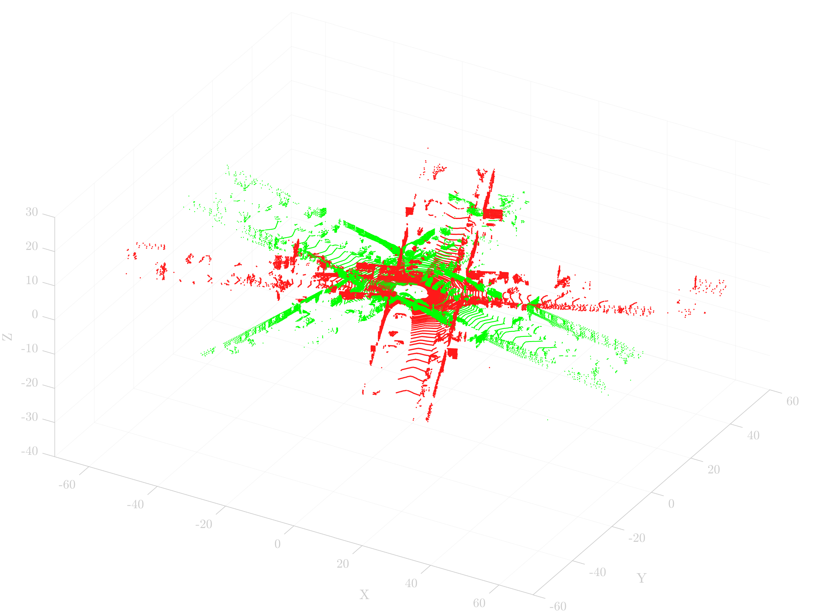
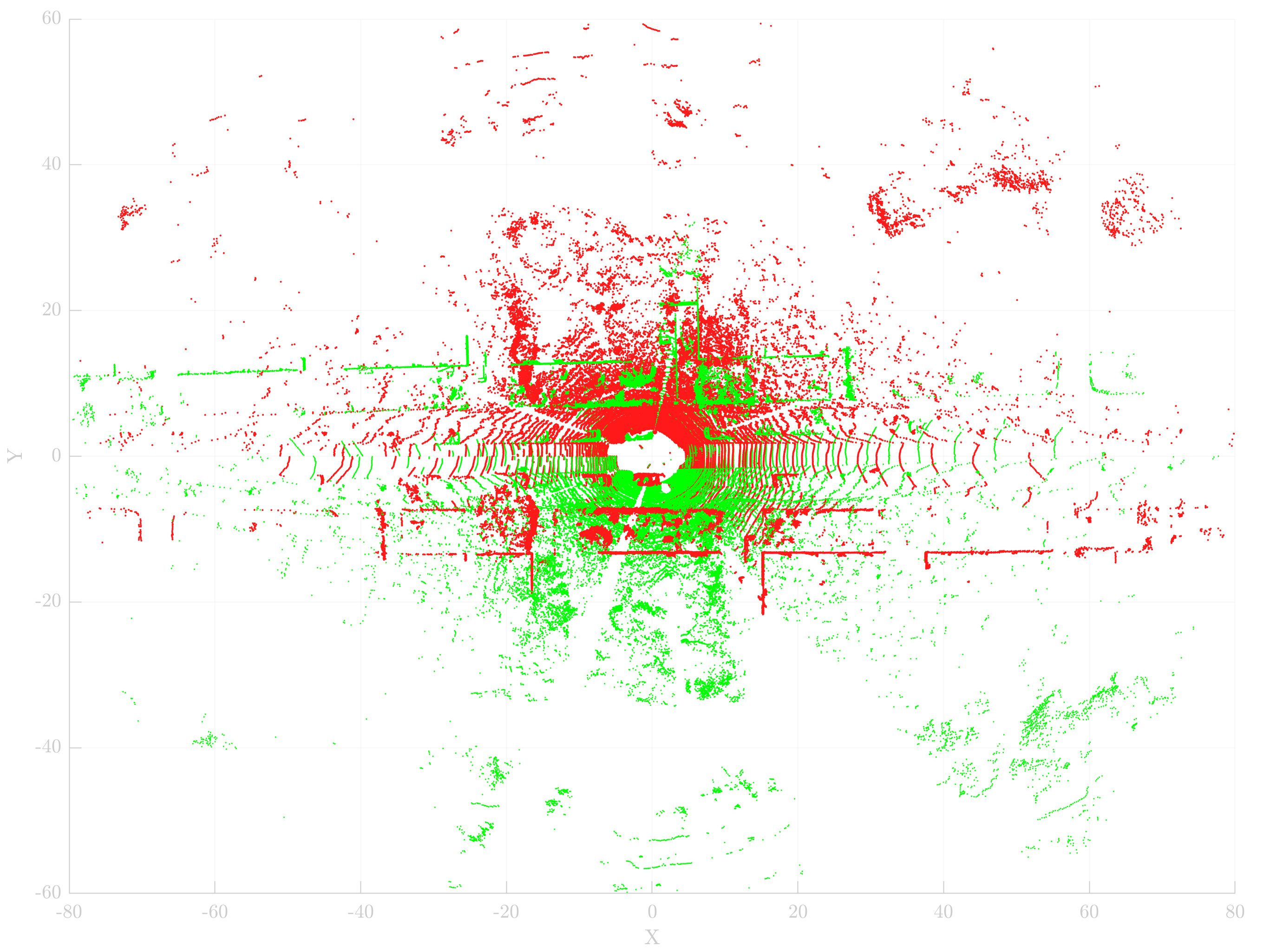
(a) Source and target

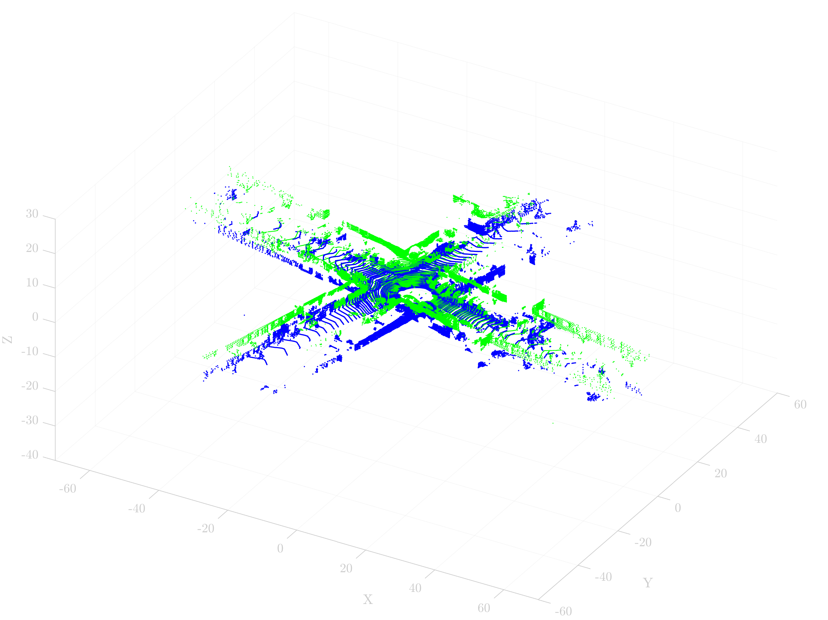
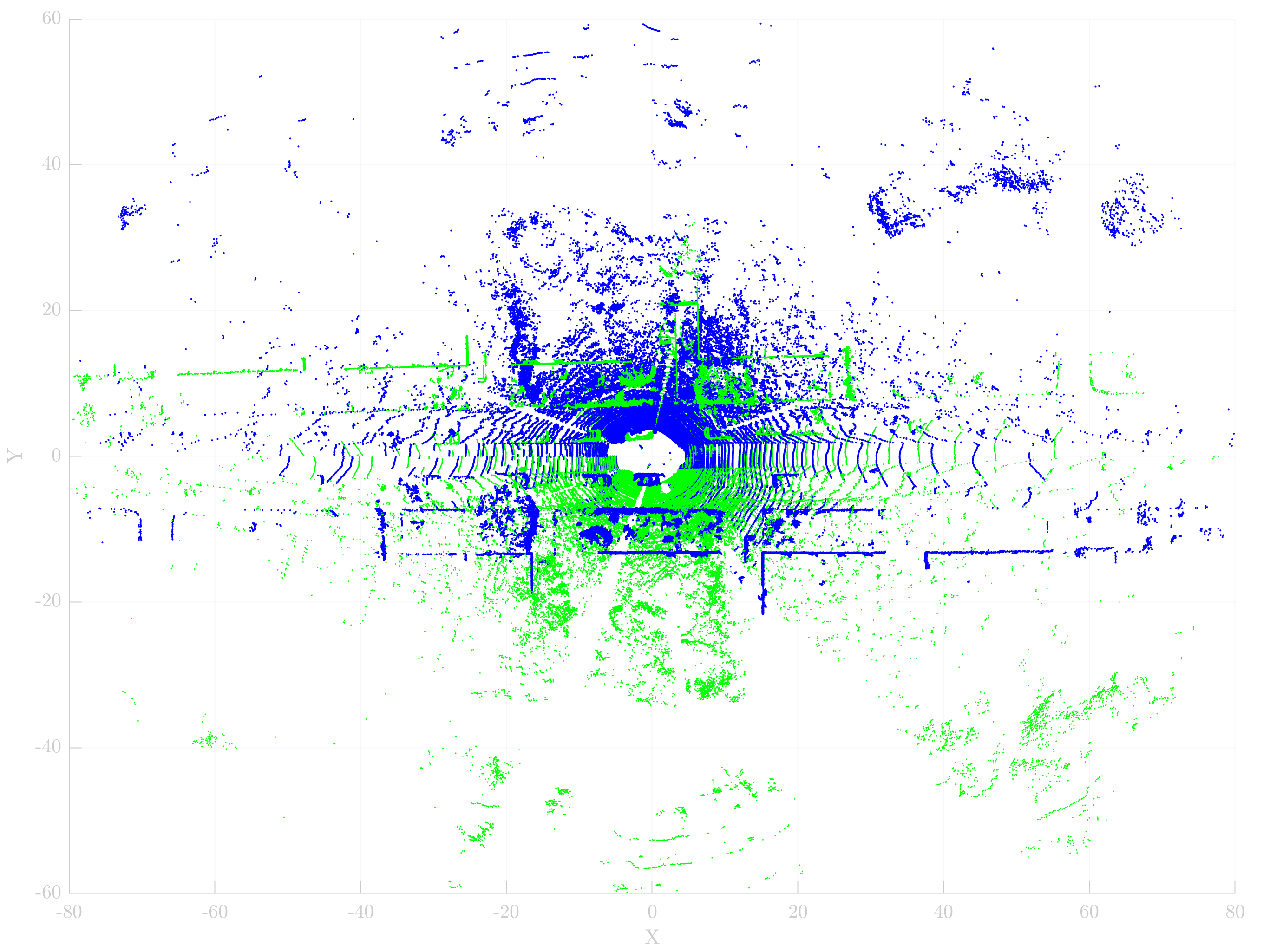
(b) RANSAC10K [23]

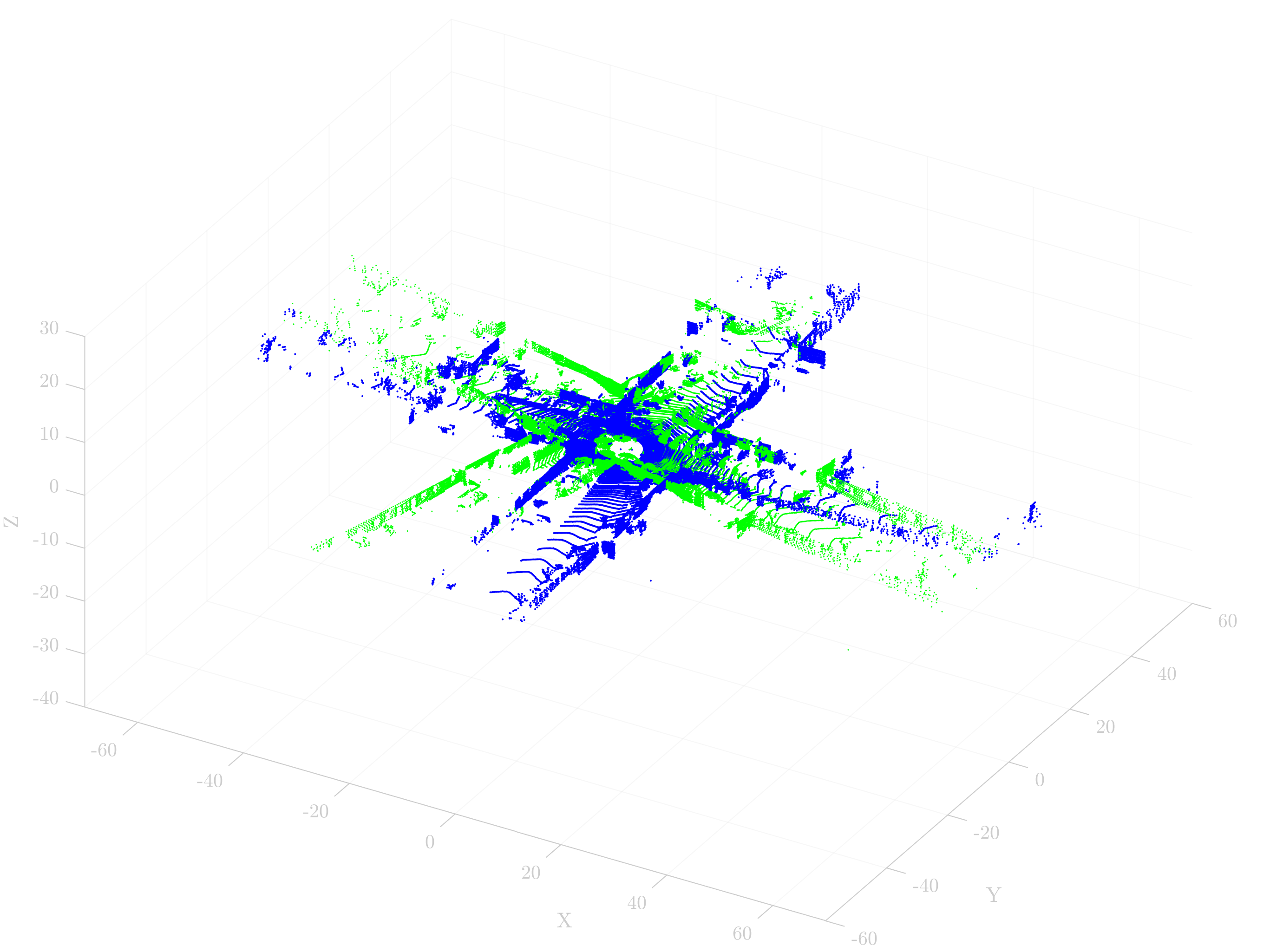
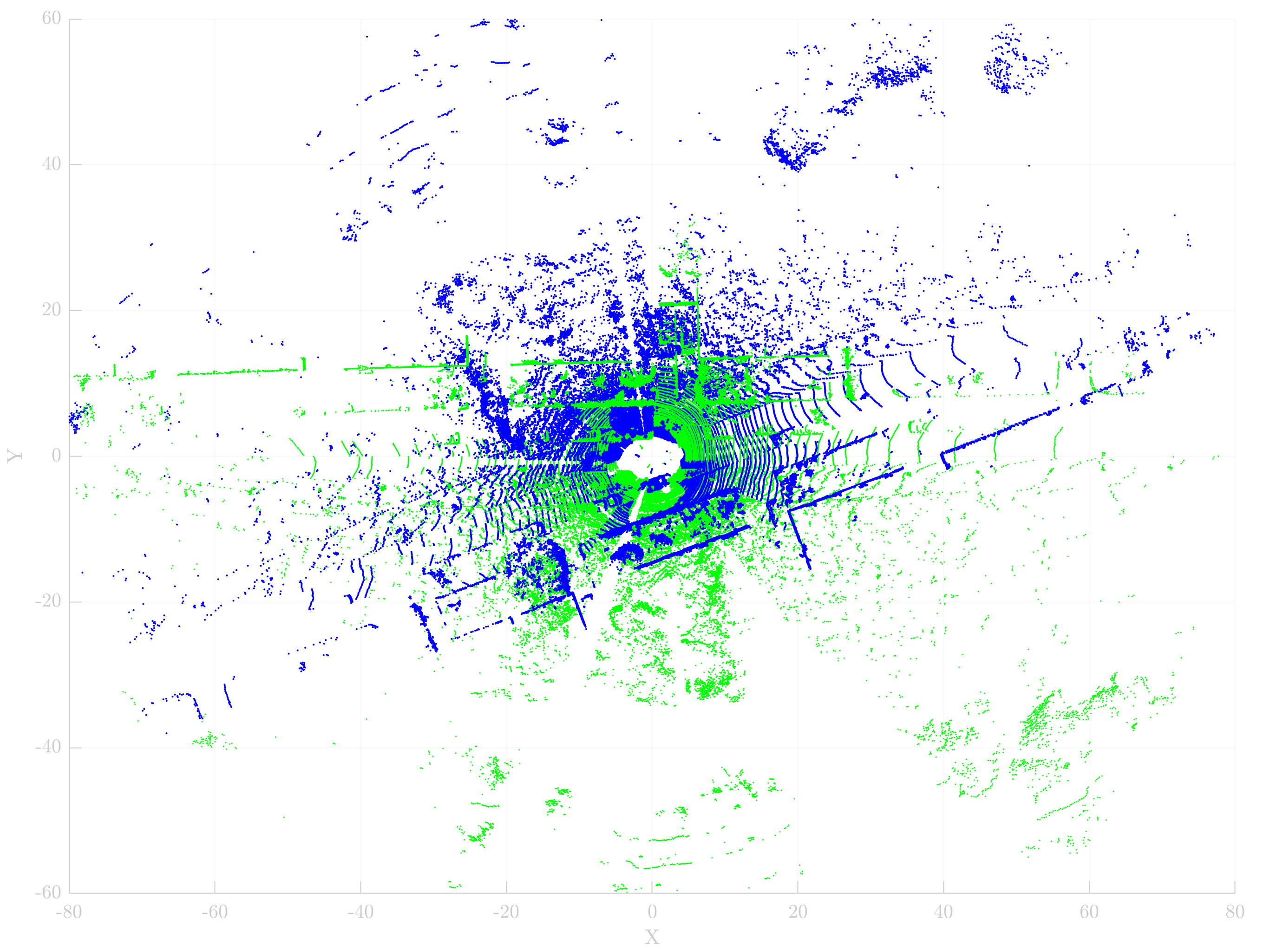
(c) FGR [26]

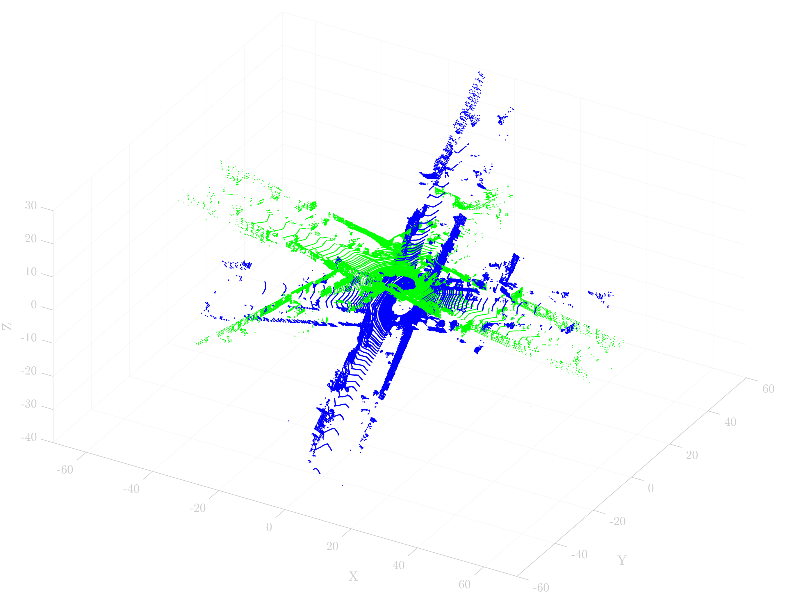
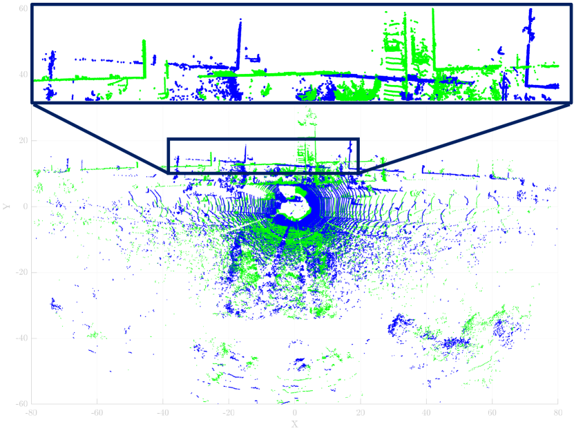
(d) TEASER++ [27]

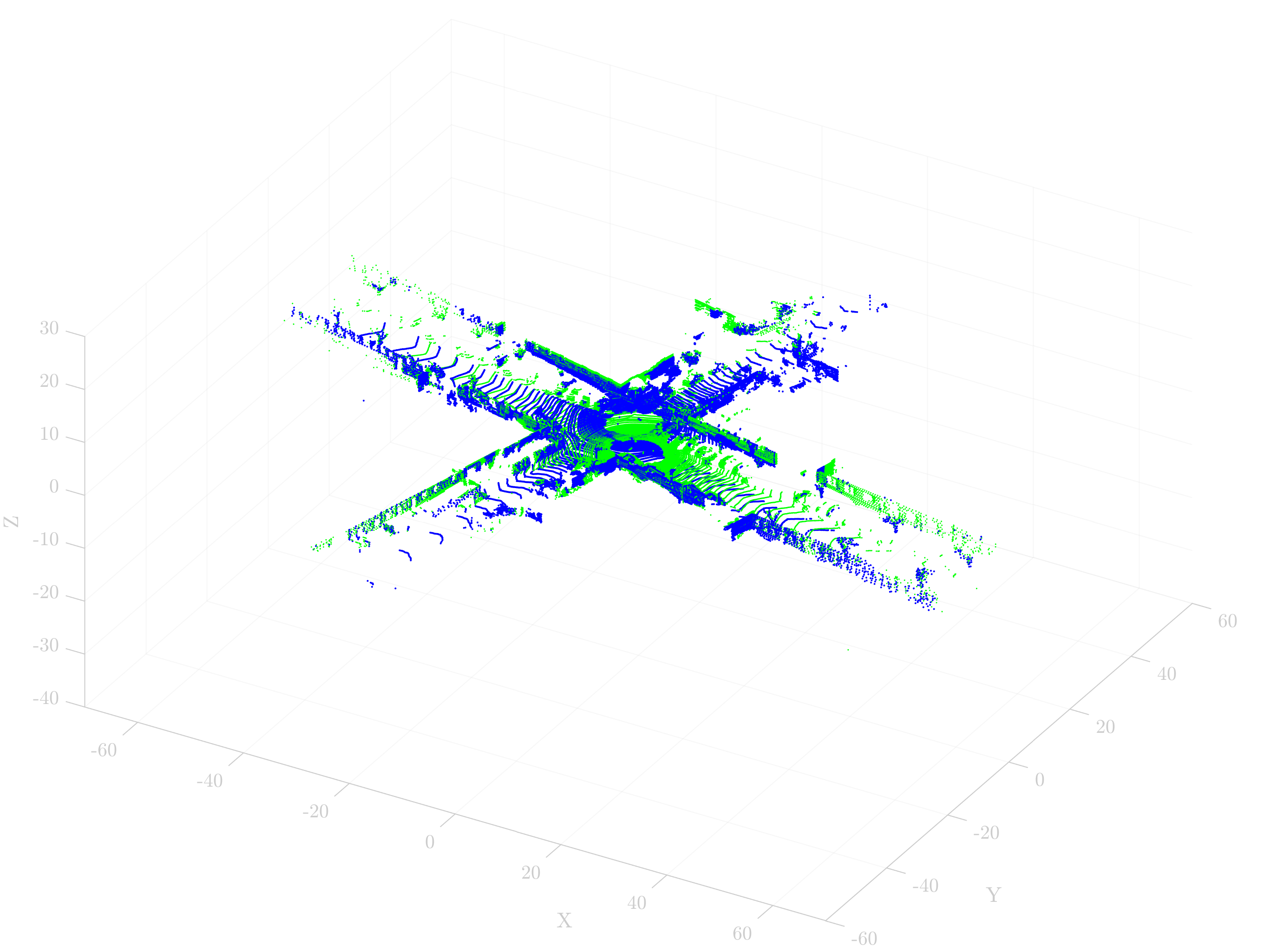
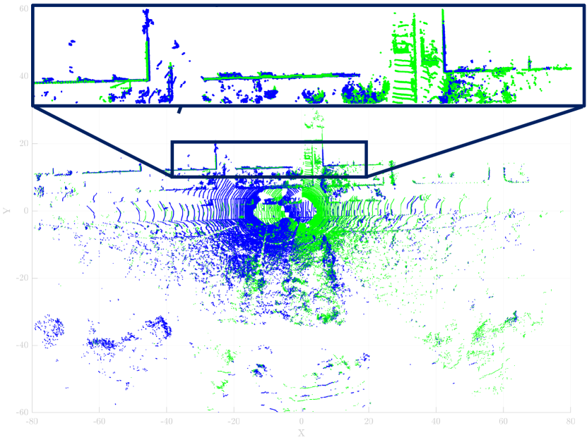
(e) Quatro (Ours)

Figure 4: Degeneracy cases (T-B): Registration results between 1,398 to 3,554 frames in Seq. 00, which are 9.88 m apart, and between 177 and 1,726 frames in Seq. 08, which are 9.82 m apart. The red, green, and blue points denote source, target, and estimate, respectively. Note that RANSAC [23] returns $\mathbf{I}_{4}$ if it fails to find correct putative correspondences. The closer the green and blue points are, the better (best viewed in color).

III Experiments

III-A Dataset

We experimented in the indoor/outdoor environments, i.e. KITTI dataset [7, 69] and NAVER LABS localization dataset [70]. In particular, we tested the algorithms in a) loop-closing situations, b) augmented rotation situations, and c) odometry situations.

III-B Error Metrics

As quantitative metrics, the average relative pose errors, $t_{\text{avg}}$ for translation and $r_{\text{avg}}$ for rotation, are used as follows:

• $t_{\text{avg}}=\sum_{n=1}^{N}(\mathbf{t}_{n,\text{GT}}-{\hat{\mathbf{t}}}_{n})^{2}/N$,

• $r_{\text{avg}}=\frac{180}{\pi}\cdot\sum_{n=1}^{N}\cos^{-1}(\frac{\operatorname{Tr}\left({\hat{\mathbf{R}}}_{n}^{\intercal}\mathbf{R}_{n,\text{GT}}\right)-1}{2})/N$

where the subscript GT denotes that the value is from the ground truth. For the odometry test, the relative odometry errors, $t_{\text{rel}}$ and $r_{\text{rel}}$, are used, which are calculated by [71].

III-C Parameters of Quatro

Empirically, we set $\bar{c}=0.15$ and $\kappa=1.4$. Because of the sparsity differences depend on the number of channels of LiDAR sensors, the parameters for voxel-sampled FPFH should be changed depending on the sensor configuration. Thus, we set $\nu=0.3\leavevmode\nobreak\ \text{m}$, radius for normal estimation $r_{\text{normal}}=0.5\leavevmode\nobreak\ \text{m}$, and radius for FPFH $r_{\text{FPFH}}=0.65\leavevmode\nobreak\ \text{m}$ in the KITTI dataset [7], and $\nu=0.1\leavevmode\nobreak\ \text{m}$, $r_{\text{normal}}=0.3\leavevmode\nobreak\ \text{m}$, and $r_{\text{FPFH}}=0.45\leavevmode\nobreak\ \text{m}$ in the NAVER LABS localization dataset [70].

IV Experimental Results

To check the effectiveness of our proposed method, Quatro was quantitatively compared with state-of-the-art methods, namely, RANSAC [23], (specifically, RANSAC1K and RANSAC10K, where each number denotes the number of iteration), FGR [26], and TEASER++ [27]. We leveraged the open-source implementations for the experiment. Quatro-c2f comprises the proposed Quatro as a coarse alignment, followed by G-ICP [20] as a fine alignment.

IV-A Impact of Quasi-SE(3) in Distant Global Registration

In general, the state-of-the-art methods estimate precise relative pose by overcoming the effect of gross outliers. However, our Quatro exhibits noticeable robustness in the case where the relative pose between two viewpoints of source and target is distant, as shown in Fig. 4 and Table I. In particular, it was observed that FGR was more likely to fail to conduct registration compared with TEASER++ and our Quatro. This is because FGR inherently uses linearization of SE(3) in optimization. Thus, if the linearization assumption does not hold, its performance becomes degraded, as shown in Fig. 5. Furthermore, FGR has no additional outlier rejection procedure, i.e. MCIS. Consequently, as the ratio of outliers increases, the performance obviously decreases.

Table I: Success rate (unit: %) for situations where distance is between 9$\sim$12 m away under the loop-closing condition in the KITTI dataset [7]. The registration result was considered successful when the transition and rotation errors were not larger than 2 m and 10^∘, respectively. The criteria were set based on [6]: a pose difference sufficient for the local registration to allow the estimate to converge toward global minima.

Method	00	02	05	06	07	08
FGR [26]	43.81	31.45	51.37	56.46	44.49	15.78
TEASER++ [27]	98.62	98.87	98.67	97.93	97.90	98.63
Quatro (Ours)	99.30	99.24	99.63	99.34	99.75	98.86

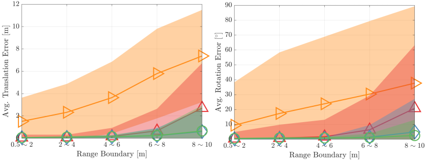
(a)

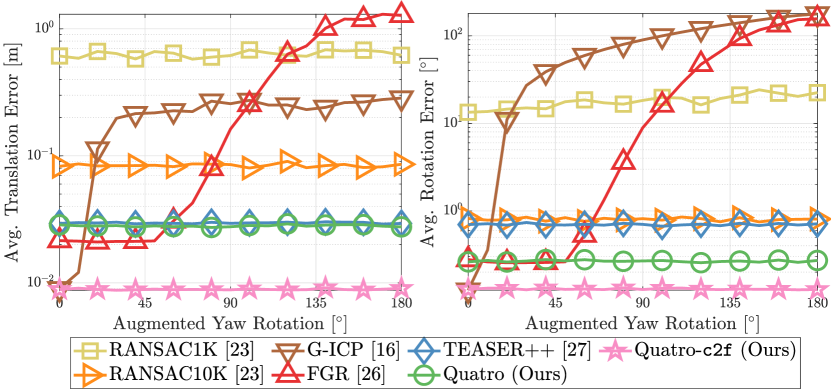
(b)

Figure 5: Performance changes with respect to (a) the range boundary in loop-closing situations in the KITTI dataset [7] and (b) the augmented yaw rotation when the frame interval is set to 5 (i.e. $\Delta 5$) in HD_B1 of the NAVER LABS localization dataset [70].

On the other hand, TEASER++, which employs MCIS similar to our proposed method, shows robust performance compared with FGR in the distant cases. Unfortunately, MCIS also occasionally rejected numerous matching pairs, so it was no longer guaranteed that there are more than three estimated inliers left in the estimating rotation. Note that TEASER++ also utilized decoupling of rotation and translation, so if TEASER++ fails to estimate the rotation, then it inevitably fails to estimate translation as a domino effect, as mentioned in Section II.E. Thus, TEASER++ shows relatively large variance as the range boundary becomes larger, compared with our Quatro, as shown in Fig. 5(a).

In particular, the variance difference between TEASER++ and Quatro in estimating rotation becomes significant, as presented in Fig. 5(a). This is because our quasi-SE(3) reduces its minimum number of the required pairs to one via quasi-SO(3) estimation and COTE. Accordingly, it successfully avoids degeneracy, even if it is given less than three estimated inliers. As a result, catastrophic failure in the rotation estimation can be somewhat prevented. Furthermore, due to the effect of the quasi-inliers, some irregular errors (i.e. $\epsilon_{k}^{\perp}$) no longer affect the estimation of $\mathbf{R}_{+}$.Thus, our method generally has a success rate of more than 99%.

Therefore, these experimental results corroborate that our quasi-SE(3) estimation enables robust global registration, while overcoming the degeneracy problem.

IV-B Comparison in Loop Closing/Odometry Test

As explained eariler, some registration methods show performance degradation as the distance or difference of rotation between two viewpoints of source and target becomes larger, as shown in Fig. 5. In contrast, our proposed method shows promising performance, especially with little variance in performance relative to other methods. Furthermore, it was shown that our quasi-SE(3) is additionally advantageous in indoor situations where the ground is mostly flat and the urban structures are orthogonal to the ground; thus, our assumption $\angle\mathbf{R}_{y}\cdot\mathbf{R}_{x}\approx\mathbf{I}_{3}$ is obviously met. As a result, our method maintains the smallest rotation error, even though source and target clouds are in diametrically opposite directions.

Furthermore, our method shows better odometry results, as shown in Table II. It is natural that local registration methods show better performance when the frame interval is small, but as the interval becomes larger, their performance drastically degraded. In contrast, the global registration methods show robust performance even though the frame interval becomes larger. In particular, performance of our method decreases little, showing smaller odometry errors than the other global registration methods.

IV-C Quatro as a Coarse Alignment

Finally, Quatro-c2f shows successful coarse-to-fine registration, as shown in Fig. 5(b) and Table II. In particular, Quatro-c2f even shows better performance compared with the state-of-the-art methods, including conventional and deep learning-based approaches in a sequence that is used as a training dataset. Therefore, we finally confirm that Quatro can provide a sufficiently accurate coarse alignment, thus helping local registration algorithms conduct fine alignment successfully.

Table II: Comparison of odometry test with the state-of-the-art methods on Seq. 00 of the KITTI dataset [7]. The results of deep learning-based methods are from [72, 73] ($t_{\text{rel}}$: %, $r_{\text{rel}}$: $\deg$/100m).

	Method	$\Delta 1$		$\Delta 3$		$\Delta 5$
		$t_{\text{rel}}$	$r_{\text{rel}}$	$t_{\text{rel}}$	$r_{\text{rel}}$	$t_{\text{rel}}$	$r_{\text{rel}}$
Local	ICP [17]	6.88	2.99	21.92	8.70	21.14	8.51
	G-ICP [18]	1.26	0.45	5.50	1.45	14.20	3.32
	VG-ICP [20]	1.03	0.30	11.83	1.65	19.11	6.32
Global	FGR [26]	2.73	0.69	7.17	1.58	14.66	4.12
	TEASER++ [27]	2.11	0.91	2.64	1.11	3.19	0.91
	Quatro (Ours)	1.45	0.41	1.38	0.24	1.94	0.46
Deep	LO-Net [74]	1.47	0.72	N/A	N/A	N/A	N/A
	LO-Net+M [74]	0.78	0.42	N/A	N/A	N/A	N/A
	DMLO† [73]	0.83	0.44	N/A	N/A	N/A	N/A
	DMLO+M† [73]	0.73	0.44	N/A	N/A	N/A	N/A
	StickyPillars†,§ [72]	0.65	0.26	0.79	0.31	1.29	0.48
Conv.	SUMA [13]	0.68	0.23	1.69	0.61	2.36	0.51
	A-LOAM [14]	0.70	0.27	0.97	0.38	31.16	12.10
	Quatro-c2f (Ours)	0.65	0.21	0.67	0.21	0.67	0.21

$\dagger$: Used for training

$\mathsection$: A-LOAM + StickyPillars

Table III: Comparison in loop-closing situations with the state-of-the-art methods on Seq. 06 of the KITTI dataset [7]. The bold and the gray-highlight denote the best and the second-best performance, respectively ($t_{\text{avg}}$: m, $r_{\text{avg}}$: $\deg$).

Method	0 $\sim$ 2m		4 $\sim$ 6m		8 $\sim$ 10m
	$t_{\text{avg}}$	$r_{\text{avg}}$	$t_{\text{avg}}$	$r_{\text{avg}}$	$t_{\text{avg}}$	$r_{\text{avg}}$
RANSAC10K [23]	2.369	14.22	5.010	27.35	8.341	33.34
FGR [26]	0.057	0.222	0.103	0.301	1.821	1.828
TEASER++ [27]	0.070	0.285	0.131	0.481	0.498	1.469
Quatro (Ours)	0.067	0.324	0.120	0.465	0.471	0.724
Quatro w/ INS (Ours)	0.059	0.207	0.101	0.230	0.429	0.346

IV-D Application: Leveraging INS in Non-flat Regions

In addition, we conducted a feasibility study on the utilization of an INS system. That is, Quasi-SO(3) estimation is followed by the estimation of roll and pitch angles via INS measurements, i.e. $\hat{\mathbf{R}}_{y}\cdot\hat{\mathbf{R}}_{x}$. As presented in Table III, even though the raw measurements were used, leveraging pitch and roll measurements reduced the rotation error effectively. Therefore, the results show the possibility of generalization of our proposed method in non-flat regions.

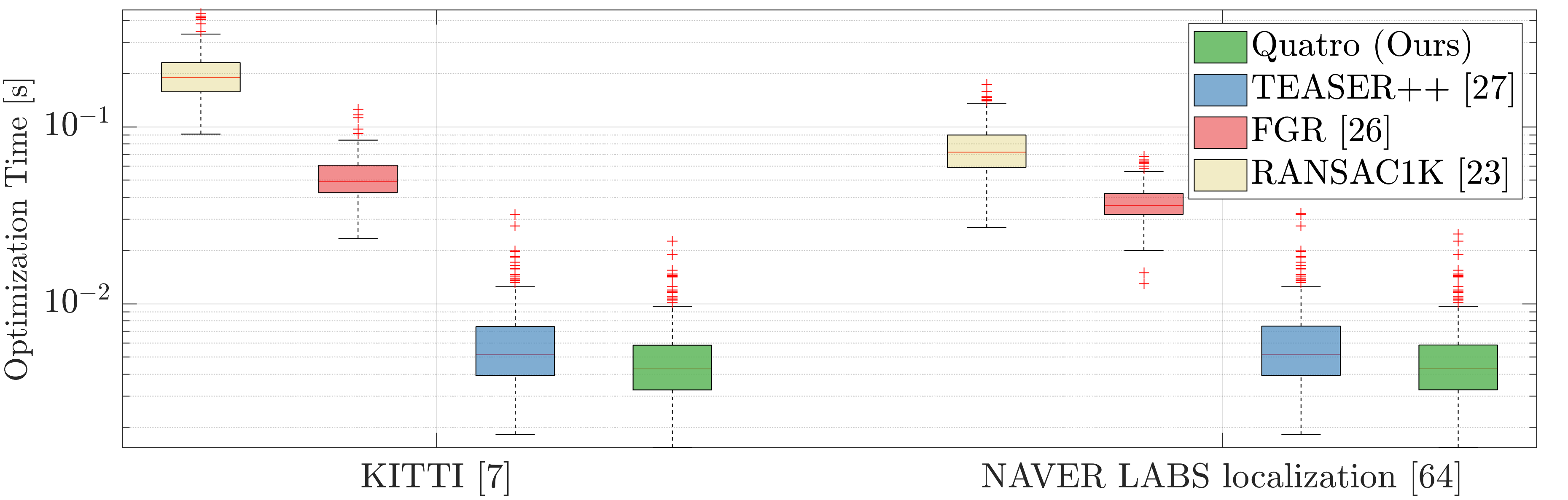
Figure 6: Average optimization time in the KITTI dataset [7] and the NAVER LABS localization dataset [70] on Intel(R) Core(TM) i9-9900KF.

IV-E Registration Speed

Furthermore, our proposed method shows the fastest optimization time by virtue of MCIS-heuristic, as represented in Fig. 6. On average, our method only takes 5 msec per optimization, which is sufficient for using our proposed method as a coarse alignment in real-time.

V Conclusion

In this study, a robust global registration method, Quatro, has been proposed. Our proposed method proved to be more robust against degeneracy compared with the state-of-the-art methods. In future works, we plan to apply the concept of Quatro for generalization on various platforms, including UAVs, backpack-type mapping systems, and so forth.

References

- [1] D. Holz, A. E. Ichim, F. Tombari, R. B. Rusu, and S. Behnke, “Registration with the point cloud library: A modular framework for aligning in 3-D,” IEEE Robot. Autom. Mag., vol. 22, no. 4, pp. 110–124, 2015.
- [2] A. Ashbrook, R. B. Fisher, C. Robertson, and N. Werghi, “Finding surface correspondence for object recognition and registration using pairwise geometric histograms,” in Proc. Eur. Conf. Comput. Vis., 1998, pp. 674–686.
- [3] C. S. Chua and R. Jarvis, “3D free-form surface registration and object recognition,” Int. J. Comput. Vis., vol. 17, no. 1, pp. 77–99, 1996.
- [4] Y. K. Cho and M. Gai, “Projection-recognition-projection method for automatic object recognition and registration for dynamic heavy equipment operations,” J. Comput. Civil Eng., vol. 28, no. 5, p. A4014002, 2014.
- [5] S. Belongie, J. Malik, and J. Puzicha, “Shape matching and object recognition using shape contexts,” IEEE Trans. Pattern Anal. Mach. Intell., vol. 24, no. 4, pp. 509–522, 2002.
- [6] H. Kim, S. Song, and H. Myung, “GP-ICP: Ground plane ICP for mobile robots,” IEEE Access, vol. 7, pp. 76 599–76 610, 2019.
- [7] A. Geiger, P. Lenz, and R. Urtasun, “Are we ready for autonomous driving? The KITTI vision benchmark suite,” in Proc. IEEE/CVF Conf. Comput. Vis. Pattern Recognit., 2012, pp. 3354–3361.
- [8] H. Lim, S. Hwang, S. Shin, and H. Myung, “Normal Distributions Transform is enough: Real-time 3D scan matching for pose correction of mobile robot under large odometry uncertainties,” in Proc. Int. Conf. Control, Automat. and Syst., 2020, pp. 1155–1161.
- [9] D. Cui, J. Xue, and N. Zheng, “Real-time global localization of robotic cars in lane level via lane marking detection and shape registration,” IEEE Trans. Intell. Transport. Syst., vol. 17, no. 4, pp. 1039–1050, 2015.
- [10] M. Javanmardi, E. Javanmardi, Y. Gu, and S. Kamijo, “Towards high-definition 3D urban mapping: Road feature-based registration of mobile mapping systems and aerial imagery,” Remote Sens., vol. 9, no. 10, p. 975, 2017.
- [11] D. Fontanelli, L. Ricciato, and S. Soatto, “A fast RANSAC-based registration algorithm for accurate localization in unknown environments using LiDAR measurements,” in Proc. IEEE Int. Conf. Autom. Sci. Eng., 2007, pp. 597–602.
- [12] S. Song and H. Myung, “Floorplan-based localization and map update using lidar sensor,” in Proc. Int. Conf. Ubiquti. Robot., 2021, pp. 30–34.
- [13] J. Behley and C. Stachniss, “Efficient surfel-based SLAM using 3D laser range data in urban environments.” in Robot. Sci. Syst., 2018.
- [14] J. Zhang and S. Singh, “LOAM: LiDAR odometry and mapping in real-time.” in Robot. Sci. Syst., vol. 2, no. 9, 2014.
- [15] G. Kim and A. Kim, “Scan context: Egocentric spatial descriptor for place recognition within 3D point cloud map,” in Proc. IEEE/RSJ Int. Conf. Intell. Robot. Syst., 2018, pp. 4802–4809.
- [16] M. Y. Chang, S. Yeon, S. Ryu, and D. Lee, “SpoxelNet: Spherical voxel-based deep place recognition for 3D point clouds of crowded indoor spaces,” in Proc. IEEE/RSJ Int. Conf. Intell. Robot. Syst., 2020, pp. 8564–8570.
- [17] P. J. Besl and N. D. McKay, “Method for registration of 3-D shapes,” in Sens. Fusion IV: Control Paradigms and Data Struct., vol. 1611, 1992, pp. 586–606.
- [18] A. Segal, D. Haehnel, and S. Thrun, “Generalized-ICP,” in Robot. Sci. Syst., vol. 2, no. 4, 2009, p. 435.
- [19] D. Chetverikov, D. Svirko, D. Stepanov, and P. Krsek, “The trimmed iterative closest point algorithm,” in Obj. Recognit. Supported by User Interact. for Serv. Robot., vol. 3, 2002, pp. 545–548.
- [20] K. Koide, M. Yokozuka, S. Oishi, and A. Banno, “Voxelized GICP for fast and accurate 3D point cloud registration,” EasyChair Preprint, no. 2703, 2020.
- [21] S. Rusinkiewicz and M. Levoy, “Efficient variants of the ICP algorithm,” in Proc. IEEE Int. Conf. on 3-D Digital Imaging and Modeling, 2001, pp. 145–152.
- [22] F. Pomerleau, F. Colas, R. Siegwart, and S. Magnenat, “Comparing ICP variants on real-world data sets,” Auton. Robot., vol. 34, no. 3, pp. 133–148, 2013.
- [23] M. A. Fischler and R. C. Bolles, “Random sample consensus: A paradigm for model fitting with applications to image analysis and automated cartography,” Commun. ACM, vol. 24, no. 6, pp. 381–395, 1981.
- [24] Z. Dong, B. Yang, Y. Liu, F. Liang, B. Li, and Y. Zang, “A novel binary shape context for 3D local surface description,” ISPRS J. of Photogramm. Remote Sens., vol. 130, pp. 431–452, 2017.
- [25] J. Yang, H. Li, D. Campbell, and Y. Jia, “Go-ICP: A globally optimal solution to 3D ICP point-set registration,” IEEE Trans. Pattern Anal. Mach. Intell., vol. 38, no. 11, pp. 2241–2254, 2015.
- [26] Q.-Y. Zhou, J. Park, and V. Koltun, “Fast global registration,” in Proc. Eur. Conf. Comput. Vis., 2016, pp. 766–782.
- [27] H. Yang, J. Shi, and L. Carlone, “TEASER: Fast and certifiable point cloud registration,” IEEE Trans. Robot., vol. 37, no. 2, pp. 314–333, 2020.
- [28] V. Tzoumas, P. Antonante, and L. Carlone, “Outlier-robust spatial perception: Hardness, general-purpose algorithms, and guarantees,” in Proc. IEEE/RSJ Int. Conf. Intell. Robot. and Syst., 2019, pp. 5383–5390.
- [29] L. Bernreiter, L. Ott, J. Nieto, R. Siegwart, and C. Cadena, “PHASER: A robust and correspondence-free global point cloud registration,” IEEE Robot. Automat. Lett., vol. 6, no. 2, pp. 855–862, 2021.
- [30] M. Rouhani and A. D. Sappa, “Correspondence free registration through a point-to-model distance minimization,” in Proc. IEEE Int. Conf. Comput. Vis., 2011, pp. 2150–2157.
- [31] M. Brown, D. Windridge, and J.-Y. Guillemaut, “A family of globally optimal branch-and-bound algorithms for 2D-3D correspondence-free registration,” Pattern Recognit., vol. 93, pp. 36–54, 2019.
- [32] C. Papazov, S. Haddadin, S. Parusel, K. Krieger, and D. Burschka, “Rigid 3D geometry matching for grasping of known objects in cluttered scenes,” Int. J. Robot. Res., vol. 31, no. 4, pp. 538–553, 2012.
- [33] O. Chum, J. Matas, and J. Kittler, “Locally optimized RANSAC,” in Joint Pattern Recognit. Symp., 2003, pp. 236–243.
- [34] S. Choi, T. Kim, and W. Yu, “Performance evaluation of RANSAC family,” J. Comput. Vis., vol. 24, no. 3, pp. 271–300, 1997.
- [35] R. Schnabel, R. Wahl, and R. Klein, “Efficient RANSAC for point-cloud shape detection,” in Comput. Graph. Forum, vol. 26, no. 2, 2007, pp. 214–226.
- [36] C. Olsson, F. Kahl, and M. Oskarsson, “Branch-and-bound methods for euclidean registration problems,” IEEE Trans. Pattern Anal. Mach. Intell., vol. 31, no. 5, pp. 783–794, 2008.
- [37] J. Pan, Z. Min, A. Zhang, H. Ma, and M. Q.-H. Meng, “Multi-view global 2D-3D registration based on branch and bound algorithm,” in Proc. IEEE Int. Conf. Robot. and Biomim., 2019, pp. 3082–3087.
- [38] R. I. Hartley and F. Kahl, “Global optimization through rotation space search,” Int. J. Comput. Vis., vol. 82, no. 1, pp. 64–79, 2009.
- [39] H. Lei, G. Jiang, and L. Quan, “Fast descriptors and correspondence propagation for robust global point cloud registration,” IEEE Trans. Image Process., vol. 26, no. 8, pp. 3614–3623, 2017.
- [40] M. J. Black and A. Rangarajan, “On the unification of line processes, outlier rejection, and robust statistics with applications in early vision,” Int. J. Comput. Vis., vol. 19, no. 1, pp. 57–91, 1996.
- [41] L. Sun, “IRON: Invariant-based highly robust point cloud registration,” arXiv preprint arXiv:2103.04357, 2021.
- [42] H. Yang, P. Antonante, V. Tzoumas, and L. Carlone, “Graduated Non-Convexity for robust spatial perception: From non-minimal solvers to global outlier rejection,” IEEE Robot. Autom. Lett., vol. 5, no. 2, pp. 1127–1134, 2020.
- [43] L. Vandenberghe and S. Boyd, “Semidefinite programming,” SIAM Review, vol. 38, no. 1, pp. 49–95, 1996.
- [44] J. Briales and J. Gonzalez-Jimenez, “Convex global 3D registration with lagrangian duality,” in Proc. IEEE/CVF Conf. Comput. Vis. Pattern Recognit., 2017, pp. 4960–4969.
- [45] H. Maron, N. Dym, I. Kezurer, S. Kovalsky, and Y. Lipman, “Point registration via efficient convex relaxation,” ACM Trans. Graph., vol. 35, no. 4, pp. 1–12, 2016.
- [46] L. Carlone, G. C. Calafiore, C. Tommolillo, and F. Dellaert, “Planar pose graph optimization: Duality, optimal solutions, and verification,” IEEE Trans. Robot., vol. 32, no. 3, pp. 545–565, 2016.
- [47] J. Shi, H. Yang, and L. Carlone, “ROBIN: a graph-theoretic approach to reject outliers in robust estimation using invariants,” arXiv preprint arXiv:2011.03659, 2020.
- [48] L. Sun, “RANSIC: Fast and highly robust estimation for rotation search and point cloud registration using invariant compatibility,” arXiv preprint arXiv:2104.09133, 2021.
- [49] K. Ebadi, M. Palieri, S. Wood, C. Padgett, and A.-A. Agha-mohammadi, “DARE-SLAM: Degeneracy-aware and resilient loop closing in perceptually-degraded environments,” arXiv preprint arXiv:2102.05117, 2021.
- [50] A. Hinduja, B.-J. Ho, and M. Kaess, “Degeneracy-aware factors with applications to underwater SLAM,” in Proc. IEEE/RSJ Int. Conf. Intell. Robot. Syst., 2019, pp. 1293–1299.
- [51] E. Westman and M. Kaess, “Degeneracy-aware imaging sonar simultaneous localization and mapping,” IEEE J. Ocean. Eng., vol. 45, no. 4, pp. 1280–1294, 2019.
- [52] H. Lim, M. Oh, and H. Myung, “Patchwork: Concentric zone-based region-wise ground segmentation with ground likelihood estimation using a 3D LiDAR sensor,” IEEE Robot. Autom. Lett., vol. 6, no. 4, pp. 6458–6465, 2021.
- [53] H. Lim, S. Hwang, and H. Myung, “ERASOR: Egocentric ratio of pseudo occupancy-based dynamic object removal for static 3D point cloud map building,” IEEE Robot. Autom. Lett., vol. 6, no. 2, pp. 2272–2279, 2021.
- [54] W. Lu, G. Wan, Y. Zhou, X. Fu, P. Yuan, and S. Song, “DeepVCP: An end-to-end deep neural network for point cloud registration,” in Proc. IEEE/CVF Int. Conf. Comput. Vis., 2019, pp. 12–21.
- [55] D.-U. Seo, H. Lim, S. Lee, and H. Myung, “PaGO-LOAM: Robust ground-optimized LiDAR odometry,” in Proc. Int. Conf. Ubiquti. Robot., 2021, Submitted.
- [56] J. Straub, O. Freifeld, G. Rosman, J. J. Leonard, and J. W. Fisher, “The Manhattan frame model—Manhattan world inference in the space of surface normals,” IEEE Trans. Pattern Anal. Mach. Intell., vol. 40, no. 1, pp. 235–249, 2017.
- [57] R. B. Rusu, N. Blodow, and M. Beetz, “Fast point feature histograms (FPFH) for 3D registration,” in Proc. IEEE Int. Conf. Robot. Autom., 2009, pp. 3212–3217.
- [58] Z. J. Yew and G. H. Lee, “3DFeat-Net: Weakly supervised local 3D features for point cloud registration,” in Proc. Eur. Conf. Comput. Vis., 2018, pp. 607–623.
- [59] B. K. Horn, “Closed-form solution of absolute orientation using unit quaternions,” J. Opt. Soc. Am. A, vol. 4, no. 4, pp. 629–642, 1987.
- [60] K. S. Arun, T. S. Huang, and S. D. Blostein, “Least-squares fitting of two 3-D point sets,” IEEE Trans. Pattern Anal. Mach. Intell., no. 5, pp. 698–700, 1987.
- [61] D. Scaramuzza, “1-Point-RANSAC structure from motion for vehicle-mounted cameras by exploiting non-holonomic constraints,” Int. J. Comput. Vis., vol. 95, no. 1, pp. 74–85, 2011.
- [62] W. Youn, H. Lim, H. S. Choi, M. B. Rhudy, H. Ryu, S. Kim, and H. Myung, “State estimation for HALE UAVs with deep-learning-aided virtual AOA/SSA sensors for analytical redundancy,” IEEE Robot. Autom. Lett., vol. 6, no. 3, pp. 5276–5283, 2021.
- [63] T. Shan, B. Englot, D. Meyers, W. Wang, C. Ratti, and D. Rus, “LIO-SAM: Tightly-coupled LiDAR inertial odometry via smoothing and mapping,” in Proc. IEEE/RSJ Int. Conf. Intell. Robot. Syst., 2020, pp. 5135–5142.
- [64] K. Lee, S.-H. Ryu, S. Yeon, H. Cho, C. Jun, J. Kang, H. Choi, J. Hyeon, I. Baek, W. Jung, et al., “Accurate continuous sweeping framework in indoor spaces with backpack sensor system for applications to 3-D mapping,” IEEE Robot. Autom. Lett., vol. 1, no. 1, pp. 316–323, 2016.
- [65] T. Qin, P. Li, and S. Shen, “VINS-Mono: A robust and versatile monocular visual-inertial state estimator,” IEEE Trans. Robot., vol. 34, no. 4, pp. 1004–1020, 2018.
- [66] H. Lim, Y. Kim, K. Jung, S. Hu, and H. Myung, “Avoiding Degeneracy for Monocular Visual SLAM with Point and Line Features,” arXiv preprint arXiv:2103.01501, 2021.
- [67] J. A. Hesch, D. G. Kottas, S. L. Bowman, and S. I. Roumeliotis, “Camera-IMU-based localization: Observability analysis and consistency improvement,” Int. J. Robot. Res., vol. 33, no. 1, pp. 182–201, 2014.
- [68] R. A. Rossi, D. F. Gleich, A. H. Gebremedhin, M. M. A. Patwary, and M. Ali, “Parallel maximum clique algorithms with applications to network analysis and storage,” arXiv preprint arXiv:1302.6256, 2013.
- [69] A. Geiger, P. Lenz, C. Stiller, and R. Urtasun, “Vision meets robotics: The KITTI dataset,” Int. J. Robot. Res., vol. 32, no. 11, pp. 1231–1237, 2013.
- [70] D. Lee, S. Ryu, S. Yeon, Y. Lee, D. Kim, C. Han, Y. Cabon, P. Weinzaepfel, N. Guérin, G. Csurka, et al., “Large-scale localization datasets in crowded indoor spaces,” in Proc. IEEE/CVF Conf. Comput. Vis. Pattern Recognit., 2021, pp. 3227–3236.
- [71] Z. Zhang and D. Scaramuzza, “A tutorial on quantitative trajectory evaluation for visual(-inertial) odometry,” in Proc. IEEE/RSJ Int. Conf. Intell. Robot. Syst., 2018.
- [72] K. Fischer, M. Simon, F. Olsner, S. Milz, H.-M. Gross, and P. Mader, “Stickypillars: Robust and efficient feature matching on point clouds using graph neural networks,” in Proc. IEEE/CVF Conf. on Comput. Vis. Pattern Recognit., 2021, pp. 313–323.
- [73] Z. Li and N. Wang, “DMLO: Deep matching LiDAR odometry,” in Proc. IEEE/RSJ Int. Conf. Intell. Robot. Syst., 2020, pp. 6010–6017.
- [74] Q. Li, S. Chen, C. Wang, X. Li, C. Wen, M. Cheng, and J. Li, “Lo-Net: Deep real-time LiDAR odometry,” in Proc. IEEE/CVF Conf. Comput. Vis. Pattern Recognit., 2019, pp. 8473–8482.