Quantum Entanglement with Generalized Uncertainty Principle

Abstract

We explore how the quantum entanglement is modified in the generalized uncertainty principle (GUP)-corrected quantum mechanics by introducing the coupled harmonic oscillator system. Constructing the ground state $\rho_{0}$ and its reduced substate $\rho_{A}=\mbox{Tr}_{B}\rho_{0}$, we compute two entanglement measures of $\rho_{0}$, i.e. ${\cal E}_{EoF}(\rho_{0})=S_{von}(\rho_{A})$ and ${\cal E}_{\gamma}(\rho_{0})=S_{\gamma}(\rho_{A})$, where $S_{von}$ and $S_{\gamma}$ are the von Neumann and Rényi entropies, up to the first order of the GUP parameter $\alpha$. It is shown that ${\cal E}_{\gamma}(\rho_{0})$ increases with increasing $\alpha$ when $\gamma=2,3,\cdots$. The remarkable fact is that ${\cal E}_{EoF}(\rho_{0})$ does not have first-order of $\alpha$. Based on there results we conjecture that ${\cal E}_{\gamma}(\rho_{0})$ increases or decreases with increasing $\alpha$ when $\gamma>1$ or $\gamma<1$ respectively for nonnegative real $\gamma$.

I Introduction

As IC (integrated circuit) becomes smaller and smaller in modern classical technology, the effect of quantum mechanics becomes prominent more and more. As a result, quantum technology (technology based on quantum mechanics and quantum information theoriestext ) becomes important more and more recently. The representative constructed by quantum technology is a quantum computersupremacy-1 , which was realized recently by making use of superconducting qubits. In quantum information processing quantum entanglementtext ; schrodinger-35 ; horodecki09 plays an important role as a physical resource. It is used in various quantum information processing, such as quantum teleportationteleportation ; Luo2019 , superdense codingsuperdense , quantum cloningclon , quantum cryptographycryptography ; cryptography2 , quantum metrologymetro17 , and quantum computersupremacy-1 ; qcreview ; computer . Furthermore, with many researchers trying to realize such quantum information processing in the laboratory for the last few decades, quantum cryptography and quantum computer seem to approaching the commercial levelwhite ; ibm .

Physics at the Planck scale suggests the existence of the minimal length (ML). The existence of the ML at this scale seems to be a universal characteristic of quantum gravitytownsend76 ; amati89 ; garay94 . It appears in loop quantum gravityrovelli88 ; rovelli90 ; rovelli98 ; carlip01 , string theorykonishi90 ; kato90 ; strominger91 , path-integral quantum gravitypadmanabhan85 ; padmanabhan85-2 ; padmanabhan86 ; padmanabhan87 ; greensite91 , and black hole physicsmaggiore93 . ML also appeared in some microscope thought-experimentmead64 . From an aspect of quantum mechanics the existence of ML modifies the uncertainty principle from Heisenberg uncertainty principle (HUP)uncertainty ; robertson1929 $\Delta P\Delta Q\geq\frac{\hbar}{2}$ to generalized uncertainty principle (GUP)kempf93 ; kempf94 . This is because of the fact that the uncertainty of the position $\Delta Q$ should be larger than the ML.

Then, it is natural to ask how the quantum entanglement is modified at the Planck scale. This question might be important to unveil the role of the quantum information at the Planck scale or early universe. In order to explore this issue we choose the GUP as the simplest form proposed in Ref. kempf94 :

$$\Delta P_{i}\Delta Q_{i}\geq\frac{\hbar}{2}\left[1+\alpha\left\{(\Delta{\bf P})^{2}+\langle\widehat{{\bf P}}\rangle^{2}\right\}+2\alpha\left\{(\Delta P_{i})^{2}+\langle\widehat{P}_{i}\rangle^{2}\right\}\right]\hskip 19.91684pt(i=1,2,\cdots,d)$$ (1)

where $\alpha$ is a GUP parameter, which has a dimension $(\mbox{momentum})^{-2}$. Using $\Delta A\Delta B\geq\frac{1}{2}|\langle[\widehat{A},\widehat{B}]\rangle|$, Eq. (1) induces the modification of the commutation relation as

$$\left[\widehat{Q}_{i},\widehat{P}_{j}\right]=i\hbar\left(\delta_{ij}+\alpha\delta_{ij}\widehat{{\bf P}}^{2}+2\alpha\widehat{P}_{i}\widehat{P}_{j}\right)$$ (2)

$$\hskip 28.45274pt\left[\widehat{Q}_{i},\widehat{Q}_{j}\right]=\left[\widehat{P}_{i},\widehat{P}_{j}\right]=0.$$

The existence of the ML can be seen in Eq. (1). If $\langle\widehat{{\bm{P}}}\rangle=0$ for simplicity, the equality of Eq. (1) yields

$$\Delta Q_{i}^{2}\geq\Delta Q_{i,min}^{2}=3\alpha\hbar^{2}\hskip 14.22636pt(i=1,2,\cdots,d)$$ (3)

which arises when $\Delta P_{j}=0\hskip 5.69046pt(j\neq i)$. If $\alpha$ is small, Eq. (2) can be solved as

$$\widehat{P}_{i}=\widehat{p}_{i}\left(1+\alpha\widehat{{\bf p}}^{2}+\alpha^{2}\widehat{{\bf p}}^{4}\right)+{\cal O}(\alpha^{3})\hskip 28.45274pt\widehat{Q}_{i}=\widehat{q}_{i}\left(1+\alpha^{2}\widehat{{\bf p}}^{4}\right)+{\cal O}(\alpha^{3})$$ (4)

where $p_{i}$ and $q_{i}$ obey the usual Heisenberg algebra $[q_{i},p_{j}]=i\hbar\delta_{ij}$. Thus, the ordering ambiguity occurs at ${\cal O}(\alpha^{2})$. We will use Eq. (4) in the following to compute the quantum entanglement within the first order of $\alpha$.

As commented before the purpose of this paper is to examine how the quantum entanglement is modified in the GUP-corrected quantum mechanics. In order to explore the issue we consider the two harmonic oscillator systems, which are coupled with each other via the quadratic term. The Hamiltonian of the system is presented in section II. In section III we derive the vacuum state $\rho_{0}$ and its reduced substate $\rho_{A}$. In this paper we adopt the entanglement measure for $\rho_{0}$ as von Neumann and Rényi entropies of the substate;

$${\cal E}_{EoF}(\rho_{0})=S_{von}(\rho_{A})=-\mbox{Tr}(\rho_{A}\ln\rho_{A})$$ (5)

$${\cal E}_{\gamma}(\rho_{0})=S_{\gamma}(\rho_{A})=\frac{1}{1-\gamma}\ln\left(\mbox{Tr}\rho_{A}^{\gamma}\right),$$

where $S_{von}$ and $S_{\gamma}$ denote the von Neumann and Rényi entropies. It is easy to show that these entanglement measures are invariant in the choice of the substate due to the Schmidt decompositiontext . The first entanglement measure is the most popular one called “entanglement of formation (EoF)”benn96 . The second measure was used in Ref. franchini08 ; its10 to explore the entanglement of the anisotropic XY spin chain with a transverse magnetic field in the various phases. In order to compute the entanglement measures in our system we compute $\mbox{Tr}\rho_{A}^{n}$ up to ${\cal O}(\alpha)$ in section IV. In section V we compute the entanglement of formation ${\cal E}_{EoF}(\rho_{0})$ and the second entanglement measure ${\cal E}_{\gamma}(\rho_{0})$ within the first order of $\alpha$ when $\gamma$ is positive integer. In this section it is shown that ${\cal E}_{\gamma}(\rho_{0})$ increases with increasing $\alpha$ when $\gamma=2,3,\cdots$. However, it is also shown that the first-order term of $\alpha$ in ${\cal E}_{EoF}(\rho_{0})$ is exactly zero. In section VI a brief conclusion is given.

II Hamiltonian

Let us consider the two coupled harmonic oscillator system, whose Hamiltonian is

$$\widehat{H}_{2}=\frac{1}{2m}\left(\widehat{P}_{1}^{2}+\widehat{P}_{2}^{2}\right)+\frac{1}{2}\left[k_{0}\left(\widehat{X}_{1}^{2}+\widehat{X}_{2}^{2}\right)+J\left(\widehat{X}_{1}-\widehat{X}_{2}\right)^{2}\right],$$ (6)

where $\left(\widehat{X}_{i},\widehat{P}_{i}\right)$ obeys the GUP (2). If we set

$$\widehat{X}_{j}=\widehat{x}_{j}\hskip 28.45274pt\widehat{P}_{j}=\widehat{p}_{j}(1+\alpha\widehat{p}_{j}^{2})\hskip 14.22636pt(j=1,2),$$ (7)

where $\left(\widehat{x}_{j},\widehat{p}_{j}\right)$ obeys the HUP, $\widehat{H}_{2}$ becomes

$$\widehat{H}_{2}=\widehat{h}_{1}+\widehat{h}_{2}+\frac{J}{2}(\widehat{x}_{1}-\widehat{x}_{2})^{2}+{\cal O}(\alpha^{2})$$ (8)

where

$$\widehat{h}_{j}=\frac{1}{2m}\left(\widehat{p}_{j}^{2}+2\alpha\widehat{p}_{j}^{4}\right)+\frac{1}{2}k_{0}\widehat{x}_{j}^{2}\hskip 14.22636pt(j=1,2).$$ (9)

Now, we introduce the new coordinates

$$\widehat{y}_{1}=\frac{1}{\sqrt{2}}(\widehat{x}_{1}+\widehat{x}_{2})\hskip 42.67912pt\widehat{y}_{2}=\frac{1}{\sqrt{2}}(-\widehat{x}_{1}+\widehat{x}_{2}).$$ (10)

Then, the Hamiltonian $\widehat{H}_{2}$ reduces to

$$\widehat{H}_{2}=\widehat{H}_{0}+\Delta\widehat{H}$$ (11)

where

$$\widehat{H}_{0}=\sum_{j=1}^{2}\left[\frac{1}{2m}\left(\widehat{\pi}_{j}^{2}+\alpha\widehat{\pi}_{j}^{4}\right)+\frac{1}{2}m\omega_{j}^{2}\widehat{y}_{j}^{2}\right]+{\cal O}(\alpha^{2})\hskip 28.45274pt\Delta\widehat{H}=\frac{3\alpha}{m}\widehat{\pi}_{1}^{2}\widehat{\pi}_{2}^{2}.$$ (12)

In eq. (12) $\widehat{\pi}_{1}$ and $\widehat{\pi}_{2}$ are the canonical momenta of $\widehat{y}_{1}$ and $\widehat{y}_{2}$, and the frequencies are

$$\omega_{1}=\sqrt{\frac{k_{0}}{m}}\hskip 28.45274pt\omega_{2}=\sqrt{\frac{k_{0}+2J}{m}}.$$ (13)

In next section we will derive the ground state for $\widehat{H}_{2}$ up to the order of $\alpha$ by treating $\Delta\widehat{H}$ as a small perturbation.

III Ground and its reduced states for $\widehat{H}_{2}$

Before we solve the Schrödinger equation for $\widehat{H}_{2}$, let us consider the one oscillator problem, whose Hamiltonian is $\widehat{H}_{1}=\frac{\widehat{p}^{2}}{2m}+\frac{\alpha}{m}\widehat{p}^{4}+\frac{1}{2}m\omega^{2}\widehat{x}^{2}+{\cal O}(\alpha^{2})$. In Ref. comment-1 the Schrödinger equation for $\widehat{H}_{1}$ is solved up to ${\cal O}(\alpha)$. For example, the $n$th eigenstate and the corresponding eigenvalue are

$$\psi_{n}(x:\alpha,\omega)=\phi_{n}(x:\omega)$$ (14)

$$+(\alpha m\hbar\omega)\bigg{[}\frac{(2n+3)\sqrt{(n+1)(n+2)}}{4}\phi_{n+2}(x:\omega)-\frac{(2n-1)\sqrt{n(n-1)}}{4}\phi_{n-2}(x:\omega)$$

$$+\frac{\sqrt{n(n-1)(n-2)(n-3)}}{16}\phi_{n-4}(x:\omega)-\frac{\sqrt{(n+1)(n+2)(n+3)(n+4)}}{16}\phi_{n+4}(x:\omega)\bigg{]}+{\cal O}(\alpha^{2})$$

$${\cal E}_{n}(\alpha,\omega)=\left(n+\frac{1}{2}\right)\hbar\omega\left[1+\frac{3(2n^{2}+2n+1)}{2(2n+1)}(\alpha m\hbar\omega)\right]+{\cal O}(\alpha^{2}),$$

where $n=0,1,2,\cdots$ and

$$\phi_{n}(x:\omega)=\frac{1}{\sqrt{2^{n}n!}}\left(\frac{m\omega}{\pi\hbar}\right)^{1/4}H_{n}\left(\sqrt{\frac{m\omega}{\hbar}}x\right)\exp\left[-\frac{m\omega}{2\hbar}x^{2}\right].$$ (15)

In Eq. (15) $H_{n}(z)$ is a $n$th-order Hermite polynomial. We assume $\phi_{m}(z:\omega)=0$ for $m<0$.

Now, let us consider the Schrödinger equation for $\widehat{H}_{0}$:

$$\widehat{H}_{0}\phi_{n_{1},n_{2}}^{(0)}(x_{1},x_{2})=E_{n_{1},n_{2}}^{(0)}\phi_{n_{1},n_{2}}^{(0)}(x_{1},x_{2}).$$ (16)

Since $\widehat{H}_{0}$ is diagonalized, the eigenvalue and the corresponding eigenfunction are

$$E_{n_{1},n_{2}}^{(0)}={\cal E}_{n_{1}}\left(\frac{\alpha}{2},\omega_{1}\right)+{\cal E}_{n_{2}}\left(\frac{\alpha}{2},\omega_{2}\right)$$ (17)

$$\phi_{n_{1},n_{2}}^{(0)}(x_{1},x_{2})=\psi_{n_{1}}\left(y_{1}:\frac{\alpha}{2},\omega_{1}\right)\psi_{n_{2}}\left(y_{2}:\frac{\alpha}{2},\omega_{2}\right).$$

If we treat $\Delta\widehat{H}$ as a small perturbation, the ground state $\Phi_{0,0}$ and its eigenvalue $E_{0,0}$ for $\widehat{H}_{2}$ become

$$E_{0,0}=\frac{\hbar}{2}(\omega_{1}+\omega_{2})+\frac{3}{8}(\alpha m\hbar^{2})(\omega_{1}+\omega_{2})^{2}+{\cal O}(\alpha^{2})$$ (18)

$$\Phi_{0,0}(x_{1},x_{2})=\phi_{0}(y_{1}:\omega_{1})\phi_{0}(y_{2}:\omega_{2})$$

$$+(\alpha m\hbar)\Bigg{[}\frac{3\sqrt{2}}{8}(\omega_{1}+\omega_{2})\left\{\phi_{0}(y_{1}:\omega_{1})\phi_{2}(y_{2}:\omega_{2})+\phi_{2}(y_{1}:\omega_{1})\phi_{0}(y_{2}:\omega_{2})\right\}$$

$$\hskip 56.9055pt-\frac{\sqrt{6}}{16}\left\{\omega_{1}\phi_{4}(y_{1}:\omega_{1})\phi_{0}(y_{2}:\omega_{2})+\omega_{2}\phi_{0}(y_{1}:\omega_{1})\phi_{4}(y_{2}:\omega_{2})\right\}$$

$$\hskip 142.26378pt-\frac{3}{4}\frac{\omega_{1}\omega_{2}}{\omega_{1}+\omega_{2}}\phi_{2}(y_{1}:\omega_{1})\phi_{2}(y_{2}:\omega_{2})\Bigg{]}+{\cal O}(\alpha^{2}).$$

Thus, the density matrix for the ground state is

$$\rho_{0}[x_{1},x_{2}:x_{1}^{\prime},x_{2}^{\prime}]$$ (19)

$$=\Phi_{0,0}(x_{1},x_{2})\Phi_{0,0}^{*}(x_{1}^{\prime},x_{2}^{\prime})$$

$$=\phi_{0}(y_{1}:\omega_{1})\phi_{0}(y_{2},\omega_{2})\phi_{0}(y_{1}^{\prime}:\omega_{1})\phi_{0}(y_{2}^{\prime}:\omega_{2})$$

$$+(\alpha m\hbar)\Bigg{\{}\phi_{0}(y_{1}:\omega_{1})\phi_{0}(y_{2},\omega_{2})\Bigg{[}\frac{3\sqrt{2}}{8}(\omega_{1}+\omega_{2})\left\{\phi_{0}(y_{1}^{\prime}:\omega_{1})\phi_{2}(y_{2}^{\prime}:\omega_{2})+\phi_{2}(y_{1}^{\prime}:\omega_{1})\phi_{0}(y_{2}^{\prime}:\omega_{2})\right\}$$

$$\hskip 156.49014pt-\frac{\sqrt{6}}{16}\left\{\omega_{1}\phi_{4}(y_{1}^{\prime}:\omega_{1})\phi_{0}(y_{2}^{\prime}:\omega_{2})+\omega_{2}\phi_{0}(y_{1}^{\prime}:\omega_{1})\phi_{4}(y_{2}^{\prime}:\omega_{2})\right\}$$

$$\hskip 199.16928pt-\frac{3}{4}\frac{\omega_{1}\omega_{2}}{\omega_{1}+\omega_{2}}\phi_{2}(y_{1}^{\prime}:\omega_{1})\phi_{2}(y_{2}^{\prime}:\omega_{2})\Bigg{]}$$

$$\hskip 227.62204pt+(y_{j}\leftrightarrow y_{j}^{\prime})\Bigg{\}}+{\cal O}(\alpha^{2})$$

where

$$y_{1}^{\prime}=\frac{1}{\sqrt{2}}(x_{1}^{\prime}+x_{2}^{\prime})\hskip 28.45274pty_{2}^{\prime}=\frac{1}{\sqrt{2}}(-x_{1}^{\prime}+x_{2}^{\prime}).$$ (20)

In order to examine the entanglement of $\rho_{0}$ we should derive its reduced substate. After long and tedious calculation one can derive the reduced state $\rho_{A}=\mbox{Tr}_{B}\rho_{0}$ in a form

$$\rho_{A}[x_{1},x_{1}^{\prime}]$$ (21)

$$\equiv\int dx_{2}\rho_{0}[x_{1},x_{2}:x_{1}^{\prime},x_{2}]$$

$$=\sqrt{\frac{2m\omega_{1}\omega_{2}}{\pi\hbar(\omega_{1}+\omega_{2})}}e^{-a(x_{1}^{2}+x_{1}^{\prime 2})+2bx_{1}x_{1}^{\prime}}\Bigg{[}1+\frac{\alpha m}{256\hbar(\omega_{1}+\omega_{2})^{5}}\Bigg{\{}g_{1}(x_{1}^{4}+x_{1}^{\prime 4})+g_{2}(x_{1}^{3}x_{1}^{\prime}+x_{1}x_{1}^{\prime 3})$$

$$\hskip 199.16928pt+g_{3}x_{1}^{2}x_{1}^{\prime 2}+g_{4}(x_{1}^{2}+x_{1}^{\prime 2})+g_{5}x_{1}x_{1}^{\prime}+g_{6}\Bigg{\}}\Bigg{]}+{\cal O}(\alpha^{2})$$

where

$$a=\frac{m}{8\hbar(\omega_{1}+\omega_{2})}(\omega_{1}^{2}+\omega_{2}^{2}+6\omega_{1}\omega_{2})\hskip 28.45274ptb=\frac{m(\omega_{1}-\omega_{2})^{2}}{8\hbar(\omega_{1}+\omega_{2})}$$ (22)

and

$$g_{1}=-m^{2}(\omega_{1}^{8}+5\omega_{1}^{7}\omega_{2}+94\omega_{1}^{6}\omega_{2}^{2}+459\omega_{1}^{5}\omega_{2}^{3}+930\omega_{1}^{4}\omega_{2}^{4}+459\omega_{1}^{3}\omega_{2}^{5}+94\omega_{1}^{2}\omega_{2}^{6}+5\omega_{1}\omega_{2}^{7}+\omega_{2}^{8})$$

$$g_{2}=4m^{2}(\omega_{1}-\omega_{2})^{2}(\omega_{1}^{6}+7\omega_{1}^{5}\omega_{2}+35\omega_{1}^{4}\omega_{2}^{2}+106\omega_{1}^{3}\omega_{2}^{3}+35\omega_{1}^{2}\omega_{2}^{4}+7\omega_{1}\omega_{2}^{5}+\omega_{2}^{6})$$

$$g_{3}=-6m^{2}(\omega_{1}-\omega_{2})^{4}(\omega_{1}^{4}+9\omega_{1}^{3}\omega_{2}+28\omega_{1}^{2}\omega_{2}^{2}+9\omega_{1}\omega_{2}^{3}+\omega_{2}^{4})$$ (23)

$$g_{4}=24\hbar m(\omega_{1}+\omega_{2})(2\omega_{1}^{6}+23\omega_{1}^{5}\omega_{2}+82\omega_{1}^{4}\omega_{2}^{2}+170\omega_{1}^{3}\omega_{2}^{3}+82\omega_{1}^{2}\omega_{2}^{4}+23\omega_{1}\omega_{2}^{5}+2\omega_{2}^{6})$$

$$g_{5}=-48\hbar m(\omega_{1}+\omega_{2})(\omega_{1}-\omega_{2})^{2}(2\omega_{1}^{4}+11\omega_{1}^{3}\omega_{2}+30\omega_{1}^{2}\omega_{2}^{2}+11\omega_{1}\omega_{2}^{3}+2\omega_{2}^{4})$$

$$g_{6}=-48\hbar^{2}(\omega_{1}+\omega_{2})^{2}(4\omega_{1}^{4}+17\omega_{1}^{3}\omega_{2}+38\omega_{1}^{2}\omega_{2}^{2}+17\omega_{1}\omega_{2}^{3}+4\omega_{2}^{4}).$$

It is useful to note

$$a+b=\frac{m(\omega_{1}+\omega_{2})}{4\hbar}\hskip 28.45274pta-b=\frac{m\omega_{1}\omega_{2}}{\hbar(\omega_{1}+\omega_{2})}.$$ (24)

Also, one can show

$$\frac{3}{16(a-b)^{2}}(2g_{1}+2g_{2}+g_{3})+\frac{1}{4(a-b)}(2g_{4}+g_{5})+g_{6}=0.$$ (25)

Using Eq. (25) one can explicitly show $\mbox{Tr}\rho_{A}=1$ within the leading order of $\alpha$, which guarantees that $\rho_{A}$ is a mixed quantum state.

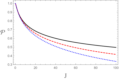
Figure 1: (Color online) The $J$-dependence of the purity function when $k_{0}=m=\hbar=1$. The black solid, red dashed, and blue dotted lines correspond to $\alpha=0$, $0.2$, and $0.4$ respectively. The figure shows that the reduced state $\rho_{A}$ becomes more mixed with increasing the GUP parameter $\alpha$.

In order to quantify how much $\rho_{A}$ is mixed we compute the purity function, whose expression is

$${\cal P}(\rho_{A})\equiv\mbox{Tr}\rho_{A}^{2}=\frac{2\sqrt{\omega_{1}\omega_{2}}}{\omega_{1}+\omega_{2}}\left[1-\frac{3\alpha m\hbar}{32}\frac{(\omega_{1}-\omega_{2})^{4}}{(\omega_{1}+\omega_{2})^{3}}+{\cal O}(\alpha^{2})\right].$$ (26)

Fig. $1$ shows the $J$-dependence of the purity function when $k_{0}=m=\hbar=1$. The black solid, red dashed, and blue dotted lines correspond to $\alpha=0$, $0.2$, and $0.4$ respectively. When $J=0$, $\rho_{A}$ is a pure state regardless of $\alpha$. With increasing $J$, $\rho_{A}$ becomes more and more mixed. The remarkable fact is that at fixed $J$ the GUP parameter $\alpha$ makes $\rho_{A}$ to be more mixed. This is due to the minus sign in the bracket of Eq. (26).

IV calculation of $\mbox{Tr}\rho_{A}^{n}$

The most typical way for computing the Rényi and von Neumann entropies of $\rho_{A}$ is to solve the eigenvalue equation

$$\int dx_{1}^{\prime}\rho_{A}[x_{1},x_{1}^{\prime}]f_{n}(x_{1}^{\prime})=\lambda_{n}f_{n}(x_{1}).$$ (27)

If $\rho_{A}$ is a Gaussian state, the eigenvalue equation (27) can be solved straightforwardlyserafini . Then, the Rényi entropy of order $\gamma$ and von Neumann entropy can be computed by making use of the eigenvalue $\lambda_{n}$ as following:

$${\cal E}_{\gamma}(\rho_{0})=\frac{1}{1-\gamma}\ln\sum_{n}\left(\lambda_{n}\right)^{\gamma}\hskip 28.45274pt{\cal E}_{EoF}(\rho_{0})=-\sum_{n}\lambda_{n}\ln\lambda_{n},$$ (28)

where $\gamma$ is arbitrary nonnegative real. The problem is that $\rho_{A}$ is not Gaussian state if $\alpha\neq 0$ as Eq. (21) shows. Thus, it seems to be extremely difficult to solve Eq. (27) directly.

Although we cannot solve the eigenvalue equation (27) explicitly, we can compute ${\cal E}_{\gamma=n}(\rho_{0})$ and ${\cal E}_{EoF}(\rho_{0})$ at least up to the ${\cal O}(\alpha)$ by computing $\mbox{Tr}\rho_{A}^{n}$ gup-sho . In this case ${\cal E}_{\gamma=n}(\rho_{0})$ can be computed by

$${\cal E}_{\gamma=n}(\rho_{0})=\frac{1}{1-n}\ln\mbox{Tr}\rho_{A}^{n}.$$ (29)

Then, ${\cal E}_{EoF}(\rho_{0})$ also can be computed from Eq. (29) by taking $n\rightarrow 1$ limit. In this reason we will compute $\mbox{Tr}\rho_{A}^{n}$ in this section within ${\cal O}(\alpha)$.

From Eq. (21) one can show

$$\mbox{Tr}\rho_{A}^{n}\equiv\int dx_{1}\cdots dx_{n}\rho_{A}[x_{1},x_{2}]\rho_{A}[x_{2},x_{3}]\cdots\rho_{A}[x_{n-1},x_{n}]\rho_{A}[x_{n},x_{1}]$$ (30)

$$\hskip 28.45274pt=\left(\frac{2m\omega_{1}\omega_{2}}{\pi\hbar(\omega_{1}+\omega_{2})}\right)^{n/2}\int dx_{1}\cdots dx_{n}\exp\left[-{\bm{X}}G_{n}{\bm{X}}^{\dagger}\right]$$

$$\times\Bigg{\{}1+\frac{\alpha m}{256\hbar(\omega_{1}+\omega_{2})^{5}}\Bigg{[}2g_{1}\left(x_{1}^{4}+\dots+x_{n}^{4}\right)$$

$$\hskip 128.0374pt+g_{2}\left[x_{1}x_{2}(x_{1}^{2}+x_{2}^{2})+\cdots+x_{n-1}x_{n}(x_{n-1}^{2}+x_{n}^{2})+x_{n}x_{1}(x_{n}^{2}+x_{1}^{2})\right]$$

$$\hskip 142.26378pt+g_{3}(x_{1}^{2}x_{2}^{2}+\cdots+x_{n-1}^{2}x_{n}^{2}+x_{n}^{2}x_{1}^{2})+2g_{4}(x_{1}^{2}+\cdots+x_{n}^{2})$$

$$\hskip 142.26378pt+g_{5}(x_{1}x_{2}+\cdots+x_{n-1}x_{n}+x_{n}x_{1})+ng_{6}\Bigg{]}+{\cal O}(\alpha^{2})\Bigg{\}},$$

where $X$ is a $n$-dimensional row vector defined by ${\bm{X}}=(x_{1},x_{2},\cdots,x_{n})$ and $G_{n}$ is a $n\times n$ matrix given by

$$G_{n}=\left(\begin{array}[]{cccccc}2a&\hskip 5.69046pt-b&&&&\hskip 5.69046pt-b\\ -b&\hskip 5.69046pt2a&\hskip 5.69046pt\bullet&&&\\ &\hskip 5.69046pt\bullet&\hskip 5.69046pt\bullet&\hskip 5.69046pt\bullet&&\\ &&\hskip 5.69046pt\bullet&\hskip 5.69046pt\bullet&\hskip 5.69046pt\bullet&\\ &&&\hskip 5.69046pt\bullet&\hskip 5.69046pt\bullet&\hskip 5.69046pt-b\\ -b&&&&\hskip 5.69046pt-b&\hskip 5.69046pt2a\end{array}\right).$$ (37)

In Eq. (37) the matrix components in the empty space are all zero. As shown in Ref. gup-sho , the determinant of $G_{n}$ is

$$\det G_{n}=2^{-n}\left[\left(\sqrt{a+b}+\sqrt{a-b}\right)^{n}-\left(\sqrt{a+b}-\sqrt{a-b}\right)^{n}\right]^{2}=\left(\frac{m}{8\hbar(\omega_{1}+\omega_{2})}\right)^{n}{\cal Z}_{-,2n}^{2}$$ (38)

where

$${\cal Z}_{\pm,\ell}=\left(\sqrt{\omega_{2}}+\sqrt{\omega_{1}}\right)^{\ell}\pm\left(\sqrt{\omega_{2}}-\sqrt{\omega_{1}}\right)^{\ell}.$$ (39)

Then, it is possible to show

$$\int dx_{1}\cdots dx_{n}\exp\left[-{\bm{X}}G_{n}{\bm{X}}^{\dagger}\right]=\frac{\pi^{n/2}}{\sqrt{\det G_{n}}}\equiv h_{n}$$ (40)

$$\int dx_{1}\cdots dx_{n}(x_{1}^{2}+\cdots+x_{n}^{2})\exp\left[-{\bm{X}}G_{n}{\bm{X}}^{\dagger}\right]$$

$$=h_{n}\frac{n}{4\sqrt{a^{2}-b^{2}}}\frac{(\sqrt{a+b}+\sqrt{a-b})^{n}+(\sqrt{a+b}-\sqrt{a-b})^{n}}{(\sqrt{a+b}+\sqrt{a-b})^{n}-(\sqrt{a+b}-\sqrt{a-b})^{n}}$$

$$=h_{n}\frac{n\hbar}{2m\sqrt{\omega_{1}\omega_{2}}}\frac{{\cal Z}_{+,2n}}{{\cal Z}_{-,2n}}$$

$$\int dx_{1}\cdots dx_{n}(x_{1}x_{2}+\cdots+x_{n-1}x_{n}+x_{n}x_{1})\exp\left[-{\bm{X}}G_{n}{\bm{X}}^{\dagger}\right]$$

$$=h_{n}\frac{nb}{2\sqrt{a^{2}-b^{2}}}\frac{(\sqrt{a+b}+\sqrt{a-b})^{n-2}+(\sqrt{a+b}-\sqrt{a-b})^{n-2}}{(\sqrt{a+b}+\sqrt{a-b})^{n}-(\sqrt{a+b}-\sqrt{a-b})^{n}}$$

$$=h_{n}\frac{n\hbar(\omega_{1}-\omega_{2})^{2}}{2m\sqrt{\omega_{1}\omega_{2}}}\frac{{\cal Z}_{+,2n-4}}{{\cal Z}_{-,2n}}.$$

Also, one can showgup-sho

$$\int dx_{1}\cdots dx_{n}(x_{1}^{4}+\cdots+x_{n}^{4})\exp\left[-{\bm{X}}G_{n}{\bm{X}}^{\dagger}\right]$$ (41)

$$=h_{n}\frac{3n}{4}\frac{(\mbox{det}H_{n-1})^{2}}{(\det G_{n})^{2}}=h_{n}\frac{3n\hbar^{2}}{4m^{2}\omega_{1}\omega_{2}}\left(\frac{{\cal Z}_{+,2n}}{{\cal Z}_{-,2n}}\right)^{2}$$

$$\int dx_{1}\cdots dx_{n}(x_{1}^{2}x_{2}^{2}+\cdots+x_{n-1}^{2}x_{n}^{2}+x_{n}^{2}x_{1}^{2})\exp\left[-{\bm{X}}G_{n}{\bm{X}}^{\dagger}\right]$$

$$=h_{n}\frac{n}{4(\det G_{n})^{2}}\Bigg{[}12a^{2}(\det H_{n-2})^{2}-12ab^{2}(\det H_{n-2})(\det H_{n-3})$$

$$\hskip 142.26378pt+3b^{4}(\det H_{n-3})^{2}-2(\det H_{n-2})(\det G_{n})\bigg{]}$$

$$=h_{n}\frac{n\hbar^{2}}{4m^{2}\omega_{1}\omega_{2}{\cal Z}_{-,2n}^{2}}\bigg{[}3{\cal Z}_{+,2n}^{2}-16(\omega_{1}+\omega_{2})\sqrt{\omega_{1}\omega_{2}}{\cal Z}_{-,4n-4}\bigg{]}$$

$$\int dx_{1}\cdots dx_{n}\left[x_{1}x_{2}(x_{1}^{2}+x_{2}^{2})+\cdots+x_{n-1}x_{n}(x_{n-1}^{2}+x_{n}^{2})+x_{n}x_{1}(x_{n}^{2}+x_{1}^{2})\right]$$

$$\hskip 227.62204pt\times\exp\left[-{\bm{X}}G_{n}{\bm{X}}^{\dagger}\right]$$

$$=h_{n}\frac{3n}{2}\frac{\left[b^{n-1}+b(\det H_{n-2})\right]\left[2a(\det H_{n-2})-b^{2}(\det H_{n-3})\right]}{(\det G_{n})^{2}}$$

$$=h_{n}\frac{3n\hbar^{2}(\omega_{1}-\omega_{2})^{2}}{2m^{2}\omega_{1}\omega_{2}}\frac{{\cal Z}_{+,2n}}{{\cal Z}_{-,2n}^{3}}\bigg{[}8(\omega_{1}+\omega_{2})\sqrt{\omega_{1}\omega_{2}}(\omega_{1}-\omega_{2})^{2(n-2)}+{\cal Z}_{-,4n-4}\bigg{]},$$

where $H_{n}$ is a $n\times n$ tridiagonal matrix given by

$$H_{n}=\left(\begin{array}[]{cccccc}2a&\hskip 5.69046pt-b&&&&\\ -b&\hskip 5.69046pt2a&\hskip 5.69046pt\bullet&&&\\ &\hskip 5.69046pt\bullet&\hskip 5.69046pt\bullet&\hskip 5.69046pt\bullet&&\\ &&\hskip 5.69046pt\bullet&\hskip 5.69046pt\bullet&\hskip 5.69046pt\bullet&\\ &&&\hskip 5.69046pt\bullet&\hskip 5.69046pt\bullet&\hskip 5.69046pt-b\\ &&&&\hskip 5.69046pt-b&\hskip 5.69046pt2a\end{array}\right).$$ (48)

It is straightforward to show

$$\det H_{n} = \frac{1}{\sqrt{a^{2}-b^{2}}}\left[a\sqrt{\det G_{2n}}-\frac{b^{2}}{2}\sqrt{\det G_{2n-2}}\right]$$

$$= \frac{1}{8(\omega_{1}+\omega_{2})\sqrt{\omega_{1}\omega_{2}}}\left(\frac{m}{8\hbar(\omega_{1}+\omega_{2})}\right)^{n}{\cal Z}_{-,4n+4}.$$

Eq. (IV) is valid for any nonnegative integer $n$.

Inserting Eqs. (40) and (41) into Eq (30), one can show that $\mbox{Tr}\rho_{A}^{n}$ can be written as a form

$$\mbox{Tr}\rho_{A}^{n}=\frac{(1-\xi)^{n}}{1-\xi^{n}}\left[1-\frac{3n(\alpha m\hbar)}{4096}\frac{(\omega_{1}-\omega_{2})^{4}}{\omega_{1}\omega_{2}(\omega_{1}+\omega_{2})^{5}}\frac{{\cal Z}_{-,4}}{{\cal Z}_{-,2n}^{2}}{\cal J}_{n}(\omega_{1},\omega_{2})+{\cal O}(\alpha^{2})\right]$$ (50)

where

$${\cal J}_{n}(\omega_{1},\omega_{2})={\cal Z}_{-,2n}\left[{\cal Z}_{+,2n+4}+2(\omega_{1}-\omega_{2})^{2}{\cal Z}_{+,2n}-2(\omega_{1}-\omega_{2})^{6}{\cal Z}_{+,2n-8}\right]$$ (51)

$$\hskip 85.35826pt-3(\omega_{1}-\omega_{2})^{2n}{\cal Z}_{-,4}-(\omega_{1}-\omega_{2})^{8}{\cal Z}_{-,4n-12}$$

and $\xi=\left[(\sqrt{\omega_{2}}-\sqrt{\omega_{1}})/(\sqrt{\omega_{2}}+\sqrt{\omega_{1}})\right]^{2}$.

It is easy to show that when $n=2$, Eq. (50) reproduces the purity function in Eq. (26). When $n=3$, Eq. (50) yields

$$\mbox{Tr}\rho_{A}^{3}=\frac{16\omega_{1}\omega_{2}}{(3\omega_{1}+\omega_{2})(\omega_{1}+3\omega_{2})}\left[1-\frac{9(\alpha m\hbar)}{4}\frac{(\omega_{1}+\omega_{2})(\omega_{1}-\omega_{2})^{4}}{(3\omega_{1}+\omega_{2})^{2}(\omega_{1}+3\omega_{2})^{2}}+{\cal O}(\alpha^{2})\right].$$ (52)

It is not difficult to show that as expected, Eq. (52) exactly coincides with $\int dx_{1}dx_{2}dx_{3}\rho_{A}[x_{1},x_{2}]\rho_{A}[x_{2},x_{3}]\rho_{A}[x_{3},x_{1}]$. In next section we will discuss on the entanglement of $\rho_{0}$ by making use of Eq. (50).

V Entanglement for $\rho_{0}$

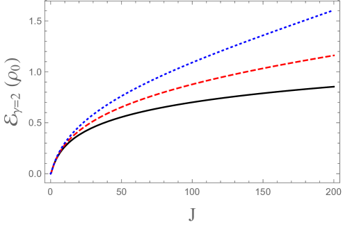
Figure 2: (Color online) The $J$-dependence of the ${\cal E}_{\gamma=2}(\rho_{0})$ when $k_{0}=m=\hbar=1$. The black solid, red dashed, and blue dotted lines correspond to $\alpha=0$, $0.2$, and $0.4$ respectively. This figure shows that it increases with increasing the GUP parameter $\alpha$.

The second entanglement measure ${\cal E}_{\gamma=n}(\rho_{0})$ can be derived by inserting Eq. (50) into Eq. (29), which is

$${\cal E}_{\gamma=n}=\frac{1}{1-n}\left[\ln\frac{(1-\xi)^{n}}{1-\xi^{n}}+\ln\left\{1-\frac{3n(\alpha m\hbar)}{4096}\frac{(\omega_{1}-\omega_{2})^{4}}{\omega_{1}\omega_{2}(\omega_{1}+\omega_{2})^{5}}\frac{{\cal Z}_{-,4}}{{\cal Z}_{-,2n}^{2}}{\cal J}_{n}(\omega_{1},\omega_{2})+{\cal O}(\alpha^{2})\right\}\right].$$ (53)

Now, let us compute the EoF of $\rho_{0}$. This is achieved by taking $n\rightarrow 1$ limit to Eq. (53). One can show that ${\cal J}_{n}(\omega_{1},\omega_{2})$ in Eq. (51) satisfies

$${\cal J}_{1}(\omega_{1},\omega_{2})=\frac{d}{dn}{\cal J}_{n}(\omega_{1},\omega_{2})\Bigg{|}_{n=1}=0.$$ (54)

Eq. (54) implies that the EoF of $\rho_{0}$ does not involve the first order of $\alpha$. Thus, it is expressed as

$${\cal E}_{EoF}(\rho_{0})=-\ln(1-\xi)-\frac{\xi}{1-\xi}\ln\xi+{\cal O}(\alpha^{2}).$$ (55)

In Fig. 2 we plot the $J$-dependence of ${\cal E}_{\gamma=2}(\rho_{0})$ when $\alpha$ is $0$ (black solid line), $0.2$ (red dashed line), and $0.4$ (blue dotted line). We set $k_{0}=m=\hbar=1$ for simplicity. This figure shows that it increases with increasing the GUP parameter $\alpha$. This can be seen from the fact that the second term in the bracket of Eq. (53) increases in the negative region with respect to $\alpha$.

VI Conclusions

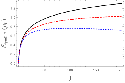
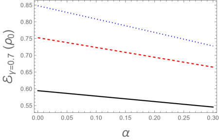
Figure 3: (Color online) (a) The $J$-dependence of the ${\cal E}_{\gamma=0.7}(\rho_{0})$ when $k_{0}=m=\hbar=1$. The black solid, red dashed, and blue dotted lines correspond to $\alpha=0$, $0.2$, and $0.4$ respectively. (b) The $\alpha$-dependence of the ${\cal E}_{\gamma=0.7}(\rho_{0})$ when $k_{0}=m=\hbar=1$. The black solid, red dashed, and blue dotted lines correspond to $J=10$, $20$, and $30$ respectively. Both figures shows that it decreases with increasing the GUP parameter $\alpha$.

In this paper we examine how the quantum entanglement is modified in the GUP-corrected quantum mechanics. In order to explore this issue we consider the coupled harmonic oscillator system. Constructing the vacuum state $\rho_{0}$ and its substate $\rho_{A}$, we compute the entanglement by choosing the EoF ${\cal E}_{EoF}(\rho_{0})=S_{von}(\rho_{A})$ and the Rényi entropy ${\cal E}_{\gamma}(\rho_{0})=S_{\gamma}(\rho_{A})$ of the substate as entanglement measures. It is shown that the second entanglement measure increases with increasing $\alpha$ when $\gamma=2,3,\cdots$. Remarkable fact is that the EoF is invariant within the first-order of $\alpha$ in quantum mechanics with HUP and GUP. Since ${\cal E}_{EoF}(\rho_{0})=\lim_{\gamma\rightarrow 1}{\cal E}_{\gamma}(\rho_{0})$, we conjecture that ${\cal E}_{\gamma}(\rho_{0})$ decreases with increasing $\alpha$ when $\gamma<1$.

In order to compute ${\cal E}_{\gamma}(\rho_{0})$ for nonnegative real $\gamma$ we should derive the eigenvalue $\lambda_{n}$ in Eq. (27). However, it seems to be highly difficult (or might be impossible) to derive the eigenvalue due to non-Gaussian nature of $\rho_{A}$. Thus, we cannot confirm our conjecture directly. If ${\cal E}_{\gamma}(\rho_{0})$ is equal to the right-hand side of Eq. (53) with changing only $n\rightarrow\gamma$ for all nonnegative real $\gamma$, it is possible to show that our conjecture is right. For example, we plot the $J$- dependence and $\alpha$-dependence of ${\cal E}_{\gamma=0.7}(\rho_{0})$ in Fig. 3(a) and Fig. 3(b) respectively. We choose various $\alpha$ in Fig. 3(a) and various J in Fig. 3(b). These two figures show that ${\cal E}_{\gamma=0.7}(\rho_{0})$ decreases with increasing $\alpha$, which is consistent with our conjecture.

The well-known example of the Planck scale is an early universe ($t\leq 10^{-43}(s)$ after big bang). However, we do not understand the role of quantum information at this early stage, in particular in the context of cosmology. We hope to explore this issue in the future.

Acknowledgments: This work was supported by the National Research Foundation of Korea(NRF) grant funded by the Korea government(MSIT) (No. 2021R1A2C1094580).

References

(1) M. A. Nielsen and I. L. Chuang, Quantum Computation and Quantum Information (Cambridge
University Press, Cambridge, England, 2000).
(2) F. Arute et al.,Quantum supremacy using a programmable superconducting processor, Nature 574 (2019) 505. Its supplementary information is given in arXiv:1910.11333.
(3) E. Schrödinger, Die gegenwärtige Situation in der Quantenmechanik, Naturwissenschaften,
23 (1935) 807.
(4) R. Horodecki, P. Horodecki, M. Horodecki, and K. Horodecki, Quantum Entanglement, Rev. Mod. Phys.
81 (2009) 865 [quant-ph/0702225] and references therein.
(5) C. H. Bennett, G. Brassard, C. Crepeau, R. Jozsa, A. Peres and W. K. Wootters, Teleporting
an Unknown Quantum State via Dual Classical and Einstein-Podolsky-Rosen Channles, Phys.Rev. Lett. 70 (1993) 1895.
(6)Y. H. Luo et al., Quantum Teleportation in High Dimensions, Phys. Rev. Lett. 123 (2019) 070505 [arXiv:1906.09697 (quant-ph)].
(7) C. H. Bennett and S. J. Wiesner, Communication via one- and two-particle operators on
Einstein-Podolsky-Rosen states, Phys. Rev. Lett. 69 (1992) 2881.
(8) V. Scarani, S. Lblisdir, N. Gisin and A. Acin, Quantum cloning, Rev. Mod. Phys. 77 (2005)
1225 [quant-ph/0511088] and references therein.
(9) A. K. Ekert , Quantum Cryptography Based on Bell’s Theorem, Phys. Rev. Lett. 67 (1991)
661.
(10) C. Kollmitzer and M. Pivk, Applied Quantum Cryptography (Springer, Heidelberg, Germany, 2010).
(11) K. Wang, X. Wang, X. Zhan, Z. Bian, J. Li, B. C. Sanders, and P. Xue, Entanglement-enhanced quantum metrology in a noisy environment, Phys. Rev. A97 (2018) 042112 [arXiv:1707.08790 (quant-ph)].
(12) T. D. Ladd, F. Jelezko, R. Laflamme, Y. Nakamura, C. Monroe, and J. L. O’Brien,
Quantum Computers, Nature, 464 (2010) 45 [arXiv:1009.2267 (quant-ph)].
(13) G. Vidal, Efficient classical simulation of slightly entangled quantum computations, Phys. Rev.
Lett. 91 (2003) 147902 [quant-ph/0301063].
(14) S. Ghernaouti-Helie, I. Tashi, T. Laenger, and C. Monyk, SECOQC Business White Paper, arXiv:0904.4073 (quant-ph).
(15) see https://www.technologyreview.com/s/609451/ibm-raises-the-bar-with-a-50-qubit-quantum-computer/.
(16) P. K. Townsend, Small-scale structure of spacetime as the origin of the gravitational constant, Phys. Rev. D 15 (1977) 2795.
(17) D. Amati, M. Ciafaloni, and G. Veneziano, Can spacetime be probed below the string size?, Phys. Lett. B 216 (1989) 41.
(18) L. J. Garay, Quantum gravity and minimum length, Int. J. Mod. Phys. A 10 (1995) 145 [gr-qc/9403008].
(19) C. Rovelli and L. Smolin, Knot Theory and Quantum Gravity, Phys. Rev. Lett. 61 1988 1155.
(20) C. Rovelli and L. Smolin, Loop space representation of quantum general relativity, Nucl. Phys. B 331 (1990) 80.
(21) C. Rovelli, Loop Quantum Gravity, Living Rev. Relativity, 1 (1998) 1 [gr-qc/9710008].
(22) S. Carlip, Quantum Gravity: a Progress Report, Rep. Prog. Phys. 64 (2001) 885 [gr-qc/0108040].
(23) K. Konishi, G. Paffuti, and P. Provero, it Minimum physical length and the generalized uncertainty principle in string theory, Phys. Lett. B 234 (1990) 276.
(24) M. Kato, Particle theories with minimum observable length and open string theory, Phys. Lett. B 245 (1990) 43.
(25) A. Strominger, Quantum Gravity and String Theory, What Have We Learned?, hep-th/9110011.
(26) T. Padmanabhan, Physical significance of planck length, Ann. Phys. 165 (1985) 38.
(27) T. Padmanabhan, Planck length as the lower bound to all physical length scales, Gen. Rel. Grav. 17 (1985) 215.
(28) T. Padmanabhan, The role of general relativity in the uncertainty principle, Class. Q. Grav. 3 (1986) 911.
(29) T. Padmanabhan, Limitations on the operational definition of spacetime events and quantum gravity, Class. Quant. Grav. 4 (1987) L107.
(30) J. Greensite, Is there a minimum length in D=4 lattice quantum gravity?, Phys. Lett. B 255 (1991) 375.
(31) M. Maggiore, A Generalized Uncertainty Principle in Quantum Gravity, Phys. Lett. B 304 (1993) 65 [hep-th/9301067].
(32) C. A. Mead, Possible Connection Between Gravitation and Fundamental Length, Phys. Rev. 135 (1964) B849.
(33) W. Heisenberg, Über den anschaulichen Inhalt der quantentheoretischen Kinematik und Mechanik, Z. Phys. 43 (1927) 172.
(34) H. P. Robertson, The Uncertainty Principle, Phys. Rev. 34 (1929) 163.
(35) A. Kempf, Uncertainty Relation in Quantum Mechanics with Quantum Group Symmetry, J. Math. Phys. 35 (1994) 4483 [hep-th/9311147].
(36) A. Kempf, G. Mangano, and R. B. Mann, Hilbert Space Representation of the Minimal Length Uncertainty Relation, Phys. Rev. D 52 (1995) 1108 [hep-th/9412167].
(37) C. H. Bennett, D. P. DiVincenzo, J. A. Smokin and W. K. Wootters,
Mixed-state entanglement and quantum error correction, Phys. Rev. A 54 (1996) 3824 [quant-ph/9604024].
(38) F. Franchini, A. R. Its, and V. E. Korepin, Renyi Entropy of the XY Spin Chain, J. Phys. A: Math. Theor. 41 (2008) 025302 [arXiv:0707.2534 (quant-ph)].
(39) A. R. Its and V. E. Korepin, Generalized Entropy of the Heisenberg Spin Chain Theor. Math. Phys. 164 (2010) 1136.
(40) DaeKil Park and Eylee Jung, Comment on “Path-integral action of a particle with the generalized uncertainty principle and correspondence with noncommutativity”, Phys. Rev. D 101 (2020) 068501 [arXiv:2002.07954 (quant-ph)].
(41) A. Serafini, Quantum Continuous Variable: A primer of Theoretical Methods (CRC Press, 2017, New York).
(42) MuSeong Kim, Mi-Ra Hwang, Eylee Jung, and DaeKil Park, Rényi and von Neumann entropies of thermal state in Generalized Uncertainty Principle-corrected harmonic oscillator, Mod. Phys. Lett. A 36 (2021) 2150250 [arXiv:2006.02717 (quant-ph)].