A smoothed particle hydrodynamics approach for phase field modeling of brittle fracture

Abstract

Fracture is a very challenging and complicated problem with various applications in engineering and physics. Although it has been extensively studied within the context of mesh-based numerical techniques, such as the finite element method (FEM), the research activity within the Smoothed Particle Hydrodynamics (SPH) community remains scarce. SPH is a particle-based numerical method used to discretize equations of continuum media. Its meshfree nature makes it ideal to simulate fracture scenarios that involve extreme deformations. However, to model fracture, SPH researchers have mostly relied on ad-hoc empirical local damage models, cohesive zone approaches, or pseudo-spring models, which come with a set of drawbacks and limitations. On the other hand, phase field models of brittle fracture have recently gained popularity in academic circles and provide significant improvements compared to previous approaches. These improvements include the derivation from fundamental fracture theories, the introduction of non-locality, and the ability to model multiple crack initiation, propagation, branching, and coalescence, in situations where no prior knowledge of the crack paths is available. Nevertheless, phase field for fracture has not been studied within SPH. In this proof-of-concept paper we develop and implement a phase field model of brittle fracture within the context of SPH. Comprehensive mathematical and implementation details are provided, and several challenging numerical examples are computed and illustrate the proposed method’s ability to accurately and efficiently simulate complex fracture scenarios.

A framework for modeling brittle fracture within SPH is proposed.

SPH is posed in a total Lagrangian formulation to eliminate tensile instability.

Cracks are regularized over a length scale using a hyperbolic phase field approach.

The hyperbolic phase field equation is compatible with explicit time integration.

Challenging problems with complex fracture paths are presented.

1 Introduction

The Smoothed Particle Hydrodynamics (SPH) is one of the oldest and well established particle methods, and has an outstanding application history in many fields. SPH was originally developed as an interpolation technique to study astrophysics related problems [1, 2], and was later extended to discretize fluid mechanics equations [3]. One of the major advantages of SPH over other existing particle methods, is that the inclusion of new physics is quite straightforward, and it can therefore be readily extended to new areas of application [4]. When it comes to solid mechanics, its ability to handle extreme material distortion makes it ideal for simulating large deformation problems, where conventional Lagrangian mesh-based techniques fail due to mesh entanglement and the need for frequent mesh updating or remeshing. Many interesting variants of the technique have been developed since it’s initial appearance, and the interested reader should consult [1, 2, 3, 5, 6, 7, 8, 4, 9, 10, 11, 12, 13] and the references therein.

Although SPH has been successfully applied to some complex problems in solid mechanics, fracture is still a challenging and open research area within the SPH community, and has not been extensively studied. This is because SPH is traditionally used to discretize equations of continuum mechanics, thus modeling of fracture and distinct crack surfaces is difficult. SPH researchers have so far relied on ad-hoc empirical local damage models, “cracking particles” approaches, pseudo-spring and virtual link approaches, and cohesive zone models. All the aforementioned techniques have undoubtedly advanced the state-of-the-art in simulating fracture within SPH. However, they come with certain limitations and drawbacks. For example, local damage [14] models are based on empirical damage laws rather than comprehensive fracture theories, and lead to mesh dependency and non-convergent results under refinement. The “cracking particles” approach [15] resembles the extended finite element method (XFEM) [16, 17], therefore the fracture surfaces need to be tracked, whereas the local enrichment of the approximation space leads to increased computational costs. In the pseudo-spring approach [18, 19, 20] the damage evolution is based on rather simple linear damage models, the softening curve of the damage law might lead to instabilities, and past research has shown that they are prone to spurious damage patterns. Finally, when it comes to cohesive zone models, the authors in [21, 22, 23] developed a continuum constitutive model featuring a cohesive fracture process zone, with an intrinsic physical length scale that helps remove the mesh dependency, while at the same time fracture surfaces do not need to be explicitly tracked. Nonetheless, kinematic enrichment is performed (similar to XFEM), which might potentially lead to increased computational times and complex implementation. Even though the aforementioned crack simulation techniques proved sufficient for certain classes of problems, it is evident that there is significant room for improvement when it comes to modeling fracture within the SPH framework.

Recently, phase field models of brittle fracture gained popularity within academic circles. Many interesting variants of the method have emerged and several challenging applications have been addressed [24, 25, 26, 27, 28, 29, 30, 31, 32, 33]. In phase field for fracture, cracks are not explicitly introduced in the solid, but instead the fracture surface is approximated by a phase field parameter that diffuses the discontinuity over a small region. The phase field parameter represents the material integrity, and it is a continuous variable that describes the smooth transition from the fully intact to the fully damaged state. The evolution of phase field, and hence of the fracture surface, is governed by a partial differential equation (PDE). Thus, a degree of non-locality is introduced, since the damage state at one point depends (through derivative information) on the states of neighboring points. The non-locality of the method leads to a well-posed mathematical model that exhibits mesh independence and convergence under refinement. At the same time, it can easily handle complicated discontinuity scenarios, such as crack initiation, propagation, coalescence, and branching, without prior knowledge of the crack paths, and without the need to embed any evolving discontinuities in the displacement field. As a result, propagating cracks are tracked automatically through the solution of the phase field PDE, which makes the method very attractive over other numerical approaches that require the explicit or implicit tracking of the discontinuities. Several approaches to phase field modeling of brittle fracture have been independently developed within the physics and mechanics communities, and for a thorough review the reader is encouraged to consult [27]. In the mechanics community, the starting point for deriving the method is the variational formulation of brittle fracture [34], which was regularized in [35], and extended Griffith’s theory of fracture [36].

Despite its many advantages, phase field modeling of brittle fracture has been mostly applied within the context of mesh-based numerical techniques, such as the finite element method (FEM) and isogeometric analysis (IGA) [24, 25, 26, 37, 27, 38, 39]. Employing particle and meshfree methods to discretize phase field equations for fracture comes with its own set of challenges, and very few relevant works can be found in the literature [40, 41, 42, 43, 44, 45, 46, 47, 48]. To the best of the authors’ knowledge, phase field models of brittle fracture have not been developed and investigated within SPH. In this proof-of-concept paper we develop a phase field model of brittle fracture suitable for SPH, and we demonstrate that phase field is a viable option to model fracture without running into issues that many of the previously used methods exhibit.

This paper is outlined as follows. In Section 2, we review the basics of SPH, with a particular emphasis on total Lagrangian SPH. In Section 3 we provide the basics of phase field modeling of brittle fracture, with a focus on hyperbolic phase field models that are amenable to explicit time integration. In Section 4 we outline the proposed SPH framework for coupling phase field for fracture with solid mechanics. Section 5 contains several challenging numerical examples. Section 6 draws conclusions and outlines future research directions.

2 SPH approximation and the Total Lagrangian SPH

2.1 Conventional SPH approximation

The SPH approach was initially proposed as a smoothed interpolation technique to deal with problems related to astrophysics [1, 2]. The fundamental principle of SPH requires the integral representation of functions. The SPH utilizes a weighted interpolation technique to approximate the value of any arbitrary function $f\equiv f(\textbf{x})$ at any arbitrary point x in Euclidean space. This is also known as the kernel approximation and can be written as [1, 2]

$$f(\textbf{x})\approxeq\int\displaylimits_{\Omega_{\textbf{x}}}f(\textbf{x}^{\prime})~{}W(r,h)~{}d\textbf{x}^{\prime},$$ (1)

where $\textbf{x}^{\prime}\in\Omega_{\textbf{x}}$ refers to the spatial coordinates of all the points located within the interpolation space $\Omega_{\textbf{x}}$ of point x. The term $W\equiv W(r,h)$, known as the kernel, represents the interpolation weights as a function of the Euclidean distance $r=|\textbf{x}-\textbf{x}^{\prime}|$ and the smoothing length $h=1.33\Delta x$, where $\Delta x$ is the initial particle spacing. The interpolant in Eq.(1) reproduces the function $f$ exactly if the kernel is a delta function; that is $W=1$ if $\textbf{x}^{\prime}=\textbf{x}$, and $W=0$ if $\textbf{x}^{\prime}\neq\textbf{x}$. In practice, the kernel is chosen to be a compactly supported function and approaches the delta function as $h\rightarrow 0$.

The essential advantage of the SPH interpolation is that it allows an exact differentiation of the interpolant to produce the derivatives of function $f$. The spatial derivatives of $f$ can be computed using the exact differentiation of the kernel as [1, 2]

$$\nabla f\approxeq\int\displaylimits_{\Omega_{\textbf{x}}}f(\textbf{x}^{\prime})~{}\nabla W~{}d\textbf{x}^{\prime}\text{.}$$ (2)

However, this kind of approximation does not vanish if the function is constant. To improve the accuracy of SPH for constant fields, Eq.(2) is rewritten by replacing $f$ with $\Phi f$, allowing for the nabla operator to be written as $\nabla(\Phi f)=\Phi\nabla f+f\nabla\Phi$. Thus, the derivative of the function becomes

$$\nabla f=\frac{1}{\Phi}\left[\nabla(\Phi f)-f\nabla\Phi\right],$$ (3)

where $\Phi$ is any differentiable field. Generally, in continuum mechanics related applications, $\Phi$ is set to be the density $\rho$ since it represents a physical quantity in the continuity equation. By doing so, one arrives at the following form of SPH approximation which delivers a zero derivative for constant functions [8]

$$\nabla f(\textbf{x})\approxeq\frac{1}{\rho(\textbf{x})}\int\displaylimits_{\Omega_{\textbf{x}}}\rho(\textbf{x}^{\prime})\left[f(\textbf{x}^{\prime})-f(\textbf{x})\right]~{}\nabla W~{}d\textbf{x}^{\prime}\text{.}$$ (4)

In a spatially discretized SPH particle domain Eq.(1) and Eq.(4) are written as

$$f_{\textbf{i}}\approxeq\sum_{\textbf{j}=1}^{N_{\textbf{i}}}f_{\textbf{j}}~{}W_{\textbf{ij}}~{}V_{\textbf{j}},$$ (5)

$$\frac{\partial f_{\textbf{i}}}{\partial x_{\textbf{i}}^{s}}\approxeq\frac{1}{\rho_{\textbf{i}}}\sum_{\textbf{j}=1}^{N_{\textbf{i}}}\rho_{\textbf{j}}~{}(f_{\textbf{j}}-f_{\textbf{i}})~{}\frac{\partial W_{\textbf{ij}}}{\partial x_{\textbf{j}}^{s}}~{}V_{\textbf{j}},$$ (6)

in which $N_{\textbf{i}}$ is the total number of particles located within the interpolation space, also known as the neighborhood, influence, or support domain, of particle i. $V_{\textbf{j}}$ is the infinitesimal volume of particle j. $W_{\textbf{ij}}$ is the kernel function relating the particles i and j, $x_{\textbf{j}}^{s}$ is the $s$ component of the spatial (or Eulerian) coordinate of particle j, and $\rho_{\mathbf{j}}$ is the density of particle j.

As noted in [49, 7, 11], the discretization scheme introduced in Eq.(5) and Eq.(6) suffers from the particle inconsistency arising from the non-homogeneous distribution of particles and truncation of the support domain near the boundaries, as seen in Fig. 1. This leads to a lack of conservation of mass, and linear and angular momentum.

Figure 1: Discretized SPH particle domain with the illustration of full and truncated supports.

A number of correction strategies to restore the particle consistency based on the kernel and gradient correction have been introduced [7, 12, 50]. For its simplicity, throughout this paper, we follow the gradient correction approach presented in [7], in which the gradient is corrected as $\tilde{\nabla}W_{\textbf{ij}}=\textbf{C}_{\textbf{i}}\cdot\nabla W_{\textbf{ij}}$.

$$\textbf{C}_{\textbf{i}}=-\left(\sum_{\textbf{j}=1}^{N_{\textbf{i}}}\left(\nabla W_{\textbf{ij}}\otimes\textbf{r}_{\textbf{ij}}\right)V_{\textbf{j}}\right)^{-1}\text{,}$$ (7)

is a second rank correction tensor, and $\textbf{r}_{\textbf{ij}}=\textbf{x}_{\textbf{i}}-\textbf{x}_{\textbf{j}}$ is the relative position vector of particles i and j. The use of $\textbf{C}_{\textbf{i}}$ ensures that the gradient of any linear velocity field is exactly evaluated. From this point forward, for brevity, we will omit the approximation sign and will use $``\nabla W_{\textbf{ij}}"$ or $``\partial W/\partial\textbf{x}"$ to refer to the corrected form of the kernel gradient $\tilde{\nabla}W_{\textbf{ij}}=\textbf{C}_{\textbf{i}}\cdot\nabla W_{\textbf{ij}}$.

2.2 SPH in Total Lagrangian form

So far, the general procedure for SPH as an approximation technique was presented. In this section, we further explore its applicability for solid mechanics related applications. It is well established that, when SPH is applied to solve the governing equations of solid mechanics, the use of Eulerian kernels (kernels defined on Eulerian coordinates) leads to the so-called tensile instability [5, 51]. Such kind of instability is observed in the form of material distortion under tensile stress state. This phenomenon was first noticed in [5] by carrying out the Von Neumann stability analysis (see [5] for detailed explanation). The authors in [5] concluded that for a stable solution the following condition should be satisfied

$$\frac{\partial^{2}W}{\partial\textbf{x}^{2}}\boldsymbol{\sigma}\leq 0,$$ (8)

where $\boldsymbol{\sigma}$ is the stress. This implies that as long as the left hand side of Eq.(8) is greater than 0 for a particle, the SPH approximation delivers unstable solutions. Several remedies have been suggested to overcome such instability. For example, [52] suggested an approach based on “Mutating the kernel” (see Section 6.6 of [52]). Since the tensile instability has a close relation with the second derivative of the kernel, using a proper kernel will result in a stable solution. However, such an approach is only effective in special cases [9]. Instead, the authors in [6] suggested the use of “stress points” in which additional computational nodes are introduced away from the original SPH particles to carry the stress information separately. However, in [53] it was noted that the use of Eulerian kernels along with the stress points does not fully mitigate the innate instability of SPH. The authors in [53] proposed the use of Lagrangian kernels which deliver a more stable solution. The difference between Eulerian and Lagrangian kernels is that the former is a function of Eulerian (or spatial) coordinates, whereas the later is established based on the Lagrangian/reference (or material) coordinates.

In the Total Lagrangian SPH (TLSPH) formalism, the kernel function and its derivatives are written as functions of the Lagrangian coordinates, thus, leading to the TLSPH approximation of an arbitrary function and its derivative as

$$f_{\textbf{i}}=\sum_{\textbf{j}=1}^{N_{\textbf{i}}}\frac{m_{0\textbf{j}}}{\rho_{0\textbf{j}}}~{}f_{\textbf{j}}~{}W_{\textbf{0ij}},$$ (9)

$$\frac{\partial f_{\textbf{i}}}{\partial X_{\textbf{i}}^{s}}=\frac{1}{\rho_{0\textbf{i}}}\sum_{\textbf{j}=1}^{N_{\textbf{i}}}m_{0\textbf{j}}~{}(f_{\textbf{j}}-f_{\textbf{i}})~{}\frac{\partial W_{0\textbf{ij}}}{\partial X_{\textbf{j}}^{s}},$$ (10)

where

$$\textbf{X}=\textbf{x}-\textbf{u}.$$ (11)

$W_{0\textbf{ij}}$, $m_{0}$, and $\rho_{0}$ are the kernel, mass, and density of the associated particle evaluated in the reference (initial) configuration, respectively. u is the displacement, and X is the Lagrangian coordinate, as depicted in Fig. 2.

Figure 2: Initial and displaced configurations in TLSPH.

One major advantage of TLSPH is that, unlike the conventional SPH, its support domain does not change and is evaluated only once at the beginning of the simulation. This decreases the computational cost considerably. However, it becomes problematic in situations where the domain distortion is such that it leads to significant changes in a particle’s neighbors. Cases like this are not considered in this paper and will be studied in subsequent works.

2.3 Governing Equations in TLSPH framework

In this section we present the governing equation of elastic dynamics in TLSPH formalism. Our primary concern is the conservation of momentum, given that the mass is constant, and the total energy is naturally conserved. In elastodynamics, the momentum balance equation in the reference configuration is written as [53]

$$\frac{d\textbf{v}}{dt}=\frac{1}{\rho_{0}}\nabla_{0}\cdot\textbf{P}+\textbf{b}_{0}\;\text{in}\;\Omega_{0},$$ (12)

where $\Omega_{0}$ is the domain of the continuum body in the reference coordinates, and v, $\textbf{b}_{0}$, and $t$, are the velocity, external force, and time, respectively. $\nabla_{0}\cdot\textbf{P}$ is the divergence of the first Piola–Kirchhoff stress tensor with respect to the reference coordinates. The first Piola–Kirchhoff stress tensor, P, is computed through an appropriate constitutive model, in which the deformation gradient is the corresponding measure of deformation. Details of the specific constitutive models employed in this work will be presented in subsequent sections. The deformation gradient is given as

$$\textbf{F}=\frac{\partial\textbf{x}}{\partial\textbf{X}}=\frac{\partial(\textbf{u}+\textbf{X})}{\partial\textbf{X}}=\frac{\partial\textbf{u}}{\partial\textbf{X}}+\textbf{I},$$ (13)

where I is the identity matrix. In order to calculate the deformation gradient for particle i we utilize the TLSPH approach as follows

$$\textbf{F}_{\textbf{i}}=\textbf{I}+\frac{1}{\rho_{0\textbf{i}}}\sum_{\textbf{j}=1}^{N_{\textbf{i}}}m_{0\textbf{j}}~{}(\textbf{u}_{\textbf{j}}-\textbf{u}_{\textbf{i}})\otimes\nabla_{0}W_{0\textbf{ij}},$$ (14)

or in index notation as

$$F^{ks}_{\textbf{i}}=\delta^{ks}+\frac{1}{\rho_{0\textbf{i}}}\sum_{\textbf{j}=1}^{N_{\textbf{i}}}m_{0\textbf{j}}~{}u^{k}_{\textbf{ji}}~{}\frac{\partial W_{0\textbf{ij}}}{\partial X_{\textbf{j}}^{s}},$$ (15)

in which $u_{\textbf{ji}}^{k}$ is the $k$ component of the displacement difference vector $\textbf{u}_{\textbf{ji}}=\textbf{u}_{\textbf{j}}-\textbf{u}_{\textbf{i}}$, and $\delta^{ks}$ is the Kronecker delta. Recall that $\partial W_{0\textbf{ij}}/\partial X_{\textbf{j}}^{s}$ is the corrected derivative of the Lagrangian kernel (see Section 2.1). Similarly, Eq.(12) can be written for particle i as [55]

$$\frac{d\textbf{v}_{\textbf{i}}}{dt}=\sum_{\textbf{j}=1}^{N_{\textbf{i}}}m_{0\textbf{j}}\left(\frac{\textbf{P}_{\textbf{i}}}{\rho^{2}_{0\textbf{i}}}+\frac{\textbf{P}_{\textbf{j}}}{\rho^{2}_{0\textbf{j}}}+\textbf{P}_{v\textbf{ij}}\right)\cdot\nabla_{0}W_{0\textbf{ij}}+\textbf{b}_{0\textbf{i}},$$ (16)

or in index notation as

$$\frac{dv^{k}_{\textbf{i}}}{dt}=\sum_{\textbf{j}=1}^{N_{\textbf{i}}}m_{0\textbf{j}}\left(\frac{P^{ks}_{\textbf{i}}}{\rho^{2}_{0\textbf{i}}}+\frac{P^{ks}_{\textbf{j}}}{\rho^{2}_{0\textbf{j}}}+P^{ks}_{v\textbf{ij}}\right)~{}\frac{\partial W_{0\textbf{ij}}}{\partial X_{\textbf{j}}^{s}}+b_{0\textbf{i}}^{k},$$ (17)

where Einstein’s summation rule is employed for the repeated index $s$. Furthermore, the artificial viscosity term $\textbf{P}_{v\textbf{ij}}=\textrm{det}(\textbf{F}_{\textbf{i}})~{}\pi_{\textbf{ij}}~{}\textbf{F}_{\textbf{i}}^{-1}$ is included to avoid numerical instabilities arising from zero-energy mode discrepancy in the form of a jump in the field variables or shock waves [56, 19, 57, 13]. Following the work of [57] we compute the coefficient $\pi_{\textbf{ij}}$ as

$$\pi_{\textbf{ij}}=\frac{1}{\rho_{0\textbf{i}}}(\beta_{2}G_{\textbf{ij}}^{2}-\beta_{1}~{}c_{0\textbf{i}}G_{\textbf{ij}}),$$ (18)

in which

$$c_{0\textbf{i}}=c_{0}=\sqrt{\frac{\kappa+\frac{4}{3}\mu}{\rho_{0}}}$$ (19)

is the speed of sound at particle i, $\kappa=E/(3(1-2\nu))$ is the bulk modulus, $\mu=E/(2(\nu+1))$ is the shear modulus, with $E$ and $\nu$ being the elastic modulus and Poisson’s ratio, respectively. $\beta_{1}$ and $\beta_{2}$ are scalar factors, and $G_{\textbf{ij}}$ is calculated as

$$G_{\textbf{ij}}=\frac{h~{}(\textbf{v}_{\textbf{i}}-\textbf{v}_{\textbf{j}})\cdot(\textbf{X}_{\textbf{i}}-\textbf{X}_{\textbf{j}})}{r^{2}_{0\textbf{ij}}+0.001h^{2}}.$$ (20)

Here, $r_{0\textbf{ij}}=|\textbf{X}_{\textbf{i}}-\textbf{X}_{\textbf{j}}|$ is the initial distance between particles i and j. In most of the numerical examples in this paper we set $\beta_{1}=0.04$ and $\beta_{2}=0$. Note that for larger values of time step and lower particle resolutions, higher $\beta_{1}$ and $\beta_{2}$ values may be necessary. It should be mentioned that the artificial viscosity introduces nonphysical dumping to the system. Thus, the smallest possible values of $\beta_{1}$ and $\beta_{2}$ are preferred.

3 Griffith’s theory of brittle fracture and the phase field approximation

(a)

(b)

Figure 3: (a) A solid body $\Omega$ with internal discontinuity $\Gamma$. (b) Approximation of the internal discontinuity by the phase field $s(\mathbf{x},t)$. $\epsilon_{0}$ is the length scale parameter that controls the width of the discontinuity.

In this section, to be self contained, we briefly present the basics of phase field modeling of brittle fracture. In the mechanics community, the prevailing models mostly originate from the variational formulation of brittle fracture [34] and the related regularized formulation [35, 27]. According to Griffith’s theory of brittle fracture [36], the fracture energy density $G_{c}$ is the amount of energy required to open a unit area of crack surface. Then, the total potential energy of an elastic body $\Omega$, being the sum of the elastic energy and the fracture energy, is given by the expression

$$\Pi_{p}(\mathbf{u},\Gamma)=\int_{\Omega}\psi_{e}(\bm{\varepsilon}({\mathbf{u}}))d\mathbf{x}+\int_{\Gamma}G_{c}d\Gamma,$$ (21)

where $\psi_{e}$ is the elastic strain energy density, the details of which will be presented in subsequent sections, $\boldsymbol{\varepsilon}$ is the infinitesimal strain tensor, and $\Gamma$ is the evolving internal discontinuity boundary which represents a set of discrete cracks. Extending this approach to dynamic problems the kinetic energy is defined as

$$\Pi_{k}(\mathbf{\dot{u}})=\frac{1}{2}\int_{\Omega}\rho~{}\dot{\textbf{u}}\cdot\dot{\textbf{u}}~{}d\mathbf{x},$$ (22)

where $\rho$ is the material density in the current configuration, and the superimposed dot denotes time differentiation. Combining the kinetic energy with the potential energy of Eq.(21) we arrive at the Lagrangian of the discrete fracture problem

$$L(\mathbf{u},\mathbf{\dot{u}},\Gamma)=\Pi_{k}(\mathbf{\dot{u}})-\Pi_{p}(\mathbf{u},\Gamma)=\int_{\Omega}\Bigg{(}\frac{1}{2}\rho~{}\dot{\textbf{u}}\cdot\dot{\textbf{u}}~{}-\psi_{e}(\boldsymbol{\varepsilon}(\mathbf{u}))\Bigg{)}d\mathbf{x}-\int_{\Gamma}G_{c}d\Gamma.$$ (23)

The Euler-Lagrange equations of this functional determine the equations of motion of the body, including the entire process of crack initiation, propagation, and branching of preexisting cracks. However, the numerical treatment is quite complex because tracking of the evolving discontinuity $\Gamma$ is required, which leads to complicated and expensive computations [24, 26]. Therefore, to circumvent the above-mentioned difficulties, the regularized expression for the fracture energy was instead proposed in [35] given as

$$\int_{\Gamma}G_{c}d\Gamma\approx\int_{\Omega}G_{c}\Bigg{(}\frac{(1-s)^{2}}{4\epsilon_{0}}+\epsilon_{0}|\nabla s|^{2}\Bigg{)}\,d\mathbf{x},$$ (24)

where $s$ is the so-called phase field parameter (or damage parameter) which represents the fracture surface $\Gamma$. It is a continuous variable that describes the smooth transition from the undamaged state ($s=1$) to the fully damaged one ($s=0$). $\epsilon_{0}$ is a parameter that has dimension of a length and controls the width of the smooth approximation of the crack (see Fig. 3). When $\epsilon_{0}\to 0$ the phase field approximation converges to the discrete fracture surface. In practice, $\epsilon_{0}$ should be sufficiently small so that the physics of the problem are not violated, but at the same time it should be greater or roughly equal to the spatial discretization size so that the crack is regularized over some finite width. To model the loss of material stiffness, the elastic strain energy density is defined as [25, 26]

$$\psi_{e}(\boldsymbol{\varepsilon},s)=s^{2}\psi_{e}^{+}+\psi_{e}^{-}.$$ (25)

$\psi_{e}^{+}$ and $\psi_{e}^{-}$ are the positive and negative parts of the elastic strain energy density, respectively, which will be defined in the next section according to the particular constitutive models employed. As can become evident from Eq.(25), crack propagation is only allowed in tension since the phase field parameter is applied only to the tensile part of the elastic strain energy. By substituting the phase field approximations for the fracture energy Eq.(24) and the elastic energy density Eq.(25) into the expression for the Lagrangian functional Eq.(23), and by deriving the corresponding Euler-Lagrange equations, we arrive at the strong form equations of motion that consist of the momentum balance presented in Eq.(12) and the phase field parameter evolution equation

$$\bigg{(}\frac{4\epsilon_{0}\psi_{e}^{+}}{G_{c}}+1\bigg{)}s-4\epsilon_{0}^{2}\nabla^{2}s=1\;\text{in}\;\Omega_{0},$$ (26)

where $\nabla^{2}s$ is the Laplacian of $s$.

Remark 1.

It can be seen that the kinetic energy term in the Lagrange energy functional is not affected by the phase field parameter $s$, which leads to conservation of mass.

In order to model the irreversibility condition (cracks do not heal) a history functional is introduced as

$$\mathcal{H}(\mathbf{X},t)=\max_{\tau<=t}(\psi_{e}^{+}(\mathbf{X},\tau)),$$ (27)

and is used in place of the tensile elastic strain energy $\psi_{e}^{+}$ in the phase field’s governing equation. The updated strong form that governs the evolution of the phase field parameter is

$$\bigg{(}\frac{4\epsilon_{0}\mathcal{H}}{G_{c}}+1\bigg{)}s-4\epsilon_{0}^{2}\nabla^{2}s=1\;\text{in}\;\Omega_{0}.$$ (28)

Finally, initial conditions need to be introduced for the history functional, i.e.

$$\mathcal{H}(\mathbf{X},0)=\mathcal{H}_{0}(\mathbf{X}).$$ (29)

The initial condition of the history functional $\mathcal{H}_{0}(\mathbf{X})$ can be used to model preexisting cracks in the domain. Eq.(28) and the corresponding initial condition Eq.(29) need to be solved together with the equations of motion (e.g. momentum balance Eq.(12)) to compute both the displacement field $\mathbf{u}(\mathbf{X},t)$ and the phase field parameter $s(\mathbf{X},t)$.

Although the aforementioned approach and its variants have been successfully applied within the context of numerical methods based on implicit time integration, they become problematic when lumped-mass explicit dynamics schemes are employed. The reason is that Eq.(28) is an elliptic PDE, and therefore a linear system needs to be solved in every time step to determine the phase field parameter. Though it is possible from an implementation point of view, the solution of an elliptic equation in every explicit step would make the approach computationally expensive. To overcome this difficulty, phase field models which include time dependency have been proposed. In [24] the phase field parameter evolves according to a parabolic PDE as

$$\frac{1}{M}\dot{s}+2s\psi_{e}^{+}-G_{c}\bigg{(}2\epsilon_{0}\nabla^{2}s+\frac{1-s}{2\epsilon_{0}}\bigg{)}=0\;\text{in}\;\Omega_{0},$$ (30)

where $M$ is a parameter controlling the rate at which local damage information diffuses into the bulk material. Clearly, when $M\to\infty$ the model approaches the standard elliptic models like the one of Eq.(26). However, Eq.(30) is a heat-equation-like PDE, and is subjected to an unfavorable CFL condition when explicit time integration is employed [58]

$$\Delta t\leq\Delta x^{2},$$ (31)

where $\Delta t$ and $\Delta x$ are time and length scales associated with the discretization. Therefore, the authors in [58] proposed a novel model in which the phase field parameter evolves according to a hyperbolic PDE by adding a second-order time derivative to the model of Eq.(30). The resulting PDE is

$$\frac{2G_{c}\epsilon_{0}}{c^{2}}\ddot{s}+\frac{1}{M}\dot{s}+2s\psi_{e}^{+}-G_{c}\bigg{(}2\epsilon_{0}\nabla^{2}s+\frac{1-s}{2\epsilon_{0}}\bigg{)}=0\;\text{in}\;\Omega_{0}.$$ (32)

$c$ is a speed limit on the propagation of the phase field parameter through the undamaged material and is taken to be equal to the sound speed given in Eq.(19). The model of Eq.(32) is subjected to the hyperbolic stability condition of

$$c\Delta t\leq\Delta x,$$ (33)

which is much less restrictive than the parabolic one (Eq.(31)), especially in the limit of $\Delta x\to 0$. To avoid any wave-like behavior due to the hyperbolic nature of the governing equation, the authors in [58] proposed an upper bound on $M$ such that the system is overdamped and the behavior of the phase field parameter is monotonic. The upper bound is given as

$$M\leq\frac{c}{2\sqrt{4G_{c}\epsilon_{0}\psi_{e}+G_{c}^{2}}}.$$ (34)

Finally, the irreversibility condition is enforced in a way similar to the elliptic problem (Eq.(27)) and the updated hyperbolic governing equation for the phase field damage parameter becomes

$$\frac{2G_{c}\epsilon_{0}}{c^{2}}\ddot{s}+\frac{1}{M}\dot{s}+2s\mathcal{H}-G_{c}\bigg{(}2\epsilon_{0}\nabla^{2}s+\frac{1-s}{2\epsilon_{0}}\bigg{)}=0\;\text{in}\;\Omega_{0},$$ (35)

with the initial condition of Eq.(29), whereas the upper bound on the parameter M becomes

$$M\leq\frac{c}{2\sqrt{4G_{c}\epsilon_{0}\mathcal{H}+G_{c}^{2}}}.$$ (36)

Traditionally, explicit time integration is used in SPH. Although there have been some efforts to develop SPH variants based on implicit time integration (e.g. [59]), the process is rather tedious and computationally expensive due to the large number of neighbors associated with each particle, and requires the solution of large linear systems. Thus, the hyperbolic version of the phase field PDE (Eq.(35)) is employed in this work.

4 Proposed framework

4.1 Governing equations

With the two previous sections at hand (Section 2 and Section 3), we present a total Lagrangian SPH framework for the solution of the coupled elastodynamics–phase field problem expressed through the following strong form governing equations,

$$\left\{\begin{array}[]{lr}\frac{d\textbf{v}}{dt}=\frac{1}{\rho_{0}}\nabla_{0}\cdot\textbf{P}+\textbf{b}_{0}&\text{in}\;\Omega_{0}\\ \frac{2G_{c}\epsilon_{0}}{c^{2}}\ddot{s}+\frac{1}{M}\dot{s}+2s\mathcal{H}-G_{c}\bigg{(}2\epsilon_{0}\nabla^{2}s+\frac{1-s}{2\epsilon_{0}}\bigg{)}=0&\text{in}\;\Omega_{0}\end{array}\right..$$ (37)

In the above-mentioned coupled problem, the first equation corresponds to the balance of linear momentum, that was briefly outlined in Section 2, whereas the second equation corresponds to the phase field (damage) parameter evolution. The solution of the phase field PDE is based upon the basics of TLSPH, and the overall solution procedure is outlined in this section. Before proceeding to the solution procedure we provide the details of the constitutive model.

4.2 Constitutive modeling

In Section 2 we presented the basics of TLSPH for discretizing solid mechanics equations in terms of the first Piola–Kirchhoff stress, whereas in Section 3 we outlined the basics of the phase field approach for brittle fracture in terms of a general elastic strain energy density $\psi_{e}$. Here, we provide the details of the elastic strain energy density and the corresponding constitutive equations based on two hyperelastic models; the isotropic Saint-Venant Kirchhoff and the neo-Hookean model. However, we would like to point out that other constitutive models can be used with the proposed framework.

4.2.1 Saint-Venant Kirchhoff

The Saint-Venant Kirchhoff model can be easily derived by extending the linear-elastic framework presented in [26] to large rotations. This is achieved by replacing the infinitesimal strain tensor with the Green–Lagrange strain tensor $\mathbf{E}=\frac{1}{2}(\mathbf{F}^{T}\mathbf{F}-\textbf{I})$. Then, the elastic strain energy density functional becomes

$$\psi_{e}=\frac{1}{2}\lambda(\text{tr}\mathbf{E})^{2}+\mu\text{tr}(\mathbf{E}^{2}),$$ (38)

where $\lambda=\kappa-\frac{2}{3}\mu$ and $\mu=E/(2(\nu+1))$ are the Lame parameters. We then define

$$\psi_{e}^{+}=\frac{1}{2}\lambda\{\text{tr}\mathbf{E}\}_{+}^{2}+\mu\text{tr}(\mathbf{E}^{+}\mathbf{E}^{+}),$$ (39)

$$\psi_{e}^{-}=\frac{1}{2}\lambda\{\text{tr}\mathbf{E}\}_{-}^{2}+\mu\text{tr}(\mathbf{E}^{-}\mathbf{E}^{-}),$$ (40)

where the following decomposition is employed

$$\mathbf{E}^{+}=\mathbf{Q}\mathbf{\Lambda}^{+}\mathbf{Q}^{T},$$ (41)

$$\mathbf{E}^{-}=\mathbf{Q}\mathbf{\Lambda}^{-}\mathbf{Q}^{T},$$ (42)

$$\mathbf{E}=\mathbf{Q}\mathbf{\Lambda}\mathbf{Q}^{T}.$$ (43)

$\Lambda=\text{diag}(\lambda_{1},\lambda_{2},\lambda_{3})$ has the eigenvalues of $\mathbf{E}$ on its diagonal, $\mathbf{Q}$ has the corresponding eigenvectors as its columns, $\Lambda^{\pm}=\text{diag}(\lambda_{1}^{\pm},\lambda_{2}^{\pm},\lambda_{3}^{\pm})$, and $\{\,.\,\}_{\pm}$ selects the $\pm$ part of its argument, i.e.

$$\{x\}_{\pm}=\left\{\begin{array}[]{lr}x&x\in\mathbb{R}^{\pm}\\ 0&\text{otherwise}\end{array}\right.\text{ .}$$ (44)

The second Piola–Kirchhoff stress can then be computed by differentiating the strain energy density $\psi_{e}$ with respect to the Green–Lagrange strain tensor $\mathbf{E}$,

$$\mathbf{S}^{\pm}=\frac{\partial\psi_{e}^{\pm}}{\partial\mathbf{E}}=\lambda~{}\{\text{tr}\mathbf{E}\}_{\pm}\textbf{I}+2\mu\textbf{E}^{\pm},$$ (45)

and

$$\mathbf{S}=s^{2}\mathbf{S}^{+}+\mathbf{S}^{-}.$$ (46)

Finally, the first Piola–Kirchhoff stress can be computed as

$$\mathbf{P}=\mathbf{F}\mathbf{S}.$$ (47)

4.2.2 Neo-Hookean

The Saint-Venant Kirchhoff model is known to exhibit instabilities in the case of strong compression [60]. Thus, for the problems in this paper involving strong compression, we employ a Neo-Hookean material. For the Neo-Hookean model we follow the presentation in [61, 42]. The positive and negative parts of the elastic strain energy density are given as

$$\psi_{e}^{+}=\left\{\begin{array}[]{lr}U(J)+\overline{\psi}_{e}(\overline{\mathbf{b}})&J\geq 1\\ \overline{\psi}_{e}(\overline{\mathbf{b}})&J<1,\end{array}\right.$$ (48)

$$\psi_{e}^{-}=\left\{\begin{array}[]{lr}0&J\geq 1\\ U(J)&J<1,\end{array}\right.$$ (49)

where

$$U(J)=\frac{1}{2}\kappa~{}\bigg{(}\frac{1}{2}(J^{2}-1)-\text{ln}J\bigg{)},$$ (50)

$$\overline{\psi}_{e}(\overline{\mathbf{b}})=\frac{1}{2}\mu\Big{(}\text{tr}\overline{\mathbf{b}}-3\Big{)},$$ (51)

$$J=\text{det}\mathbf{F},$$ (52)

$$\mathbf{b}=\mathbf{F}\mathbf{F}^{T},$$ (53)

$$\overline{\mathbf{b}}=J\,^{-2/3}\mathbf{b}.$$ (54)

The second Piola–-Kirchhoff stress can then be computed as

$$\mathbf{S}=2\frac{\partial\psi_{e}}{\partial\mathbf{b}}.$$ (55)

For the given elastic strain energy density this results in

$$\mathbf{S}=2\left\{\begin{array}[]{lr}s^{2}\bigg{(}U^{\prime}(J)\frac{\partial J}{\partial\mathbf{b}}+\frac{\partial\overline{\psi}_{e}(\overline{\mathbf{b})}}{\partial\mathbf{b}}\bigg{)}&J\geq 1\\ U^{\prime}(J)\frac{\partial J}{\partial\mathbf{b}}+s^{2}\frac{\partial\overline{\psi}_{e}(\overline{\mathbf{b})}}{\partial\mathbf{b}}&J<1.\end{array}\right.$$ (56)

The derivatives in the above expression are computed as

$$U^{\prime}(J)=\frac{1}{2}\kappa\Big{(}J-J^{-1}\Big{)},$$ (57)

$$\frac{\partial J}{\partial\mathbf{b}}=\frac{\partial\sqrt{\text{det}\mathbf{b}}}{\partial\mathbf{b}}=\frac{1}{2}J\mathbf{b}^{-1},$$ (58)

$$\frac{\partial\overline{\psi}_{e}}{\partial\mathbf{b}}=\frac{\partial\overline{\psi}_{e}}{\partial\overline{\mathbf{b}}}\frac{\partial\overline{\mathbf{b}}}{\partial\mathbf{b}}=\frac{J^{-2/3}}{2}\mu\bigg{(}\mathbf{I}-\frac{1}{3}\big{(}\text{tr}\mathbf{b}\big{)}\mathbf{b}^{-1}\bigg{)}.$$ (59)

Substituting the above equations into Eq.(56) we get

$$\mathbf{S}=\left\{\begin{array}[]{lr}s^{2}\bigg{(}\frac{1}{2}\kappa\big{(}J^{2}-1\big{)}\mathbf{b}^{-1}+J^{-2/3}\mu\Big{(}\mathbf{I}-\frac{1}{3}\big{(}\text{tr}\mathbf{b}\big{)}\mathbf{b}^{-1}\Big{)}\bigg{)}&J\geq 1\\ \frac{1}{2}\kappa\big{(}J^{2}-1\big{)}\mathbf{b}^{-1}+s^{2}\bigg{(}J^{-2/3}\mu\Big{(}\mathbf{I}-\frac{1}{3}\big{(}\text{tr}\mathbf{b}\big{)}\mathbf{b}^{-1}\Big{)}\bigg{)}&J<1.\end{array}\right.$$ (60)

Finally, the first Piola–Kirchhoff stress is computed as in Eq.(47).

4.3 Solution procedure and numerical implementation

We first define two common terms that will be used regularly throughout this paper, the soft particle and the phase field limit.

Definition 1.

Soft (damaged) particle refers to any SPH particle whose phase field parameter drops sufficiently so that its stress is fairly low, and thus the effect on neighboring particles is negligible. From a numerical implementation point of view, soft particles behave as rigid objects having inertia but no internal force.

Definition 2.

The phase field limit refers to the threshold value of the phase field parameter below which the particle is assumed to be a soft particle.

In order to compute the first Piola–Kirchhoff stress through the constitutive model presented in the previous subsection, we redefine the deformation gradient as

$$\textbf{F}_{\textbf{i}}=\left\{\begin{array}[]{lr}\frac{\partial\textbf{u}_{\textbf{i}}}{\partial\textbf{X}_{\textbf{i}}}+\textbf{I}&s_{\textbf{i}}>s_{l}\\ \textbf{I}&\text{otherwise}\end{array}\right.\text{~{}}{.}$$ (61)

Here $s_{l}$ is the phase field limit that determines the particle’s stiffness state and $\partial\textbf{u}_{\textbf{i}}/\partial\textbf{X}_{\textbf{i}}$ is calculated utilizing the corrected form of the TLSPH approach (see Section 2.3) as

$$\frac{\partial u^{k}_{\textbf{i}}}{\partial X^{s}_{\textbf{i}}}=\frac{1}{\rho_{0\textbf{i}}}\sum_{\textbf{j}=1}^{N}m_{0\textbf{j}}~{}u^{k}_{\textbf{ji}}~{}\frac{\partial W_{0\textbf{ij}}}{\partial X_{\textbf{j}}^{s}},$$ (62)

where $u_{\textbf{ji}}^{k}$ is the $k$ component of the displacement difference vector $\textbf{u}_{\textbf{ji}}=\textbf{u}_{\textbf{j}}-\textbf{u}_{\textbf{i}}$ between particles i and j. The kernel function in Eq.(62), and in any other calculation involving SPH interpolation, is chosen to be a cubic spline [62] defined in reference coordinates as

$$W_{0\textbf{ij}}=\left\{\begin{array}[]{ll}0&q>2\\ \frac{1}{4}C~{}(2-q)^{3}&1\leq q\leq 2\\ C~{}(1-1.5q^{2}+0.75q^{3})&0\leq q\leq 1\end{array}\right.\text{~{}}{,}$$ (63)

in which $q=|\textbf{X}_{\textbf{i}}-\textbf{X}_{\textbf{j}}|/h$ and C is a constant determined as

$$C=\left\{\begin{array}[]{ll}2/(3h)&\text{for one dimensional space}\\ 10/(7\pi h^{2})&\text{for two dimensional space}\\ 1/(\pi h^{3})&\text{for three dimensional space}\end{array}\right.\text{~{}}{,}$$ (64)

where $h$ is the smoothing length. We further rearrange Eq.(35) as

$$\ddot{s}=\frac{c^{2}}{2G_{c}\epsilon_{0}}\left[G_{c}\bigg{(}2\epsilon_{0}\nabla^{2}s+\frac{1-s}{2\epsilon_{0}}\bigg{)}-\frac{1}{M}\dot{s}-2s\mathcal{H}\right]$$ (65)

in order to have an explicit definition of the phase field inertia $\ddot{s}$, in terms of the phase field parameter $s$, its time derivative $\dot{s}$, and its Laplacian $\nabla^{2}s$. The Laplacian of the phase field is calculated utilizing the SPH Laplacian operator [63] in TLSPH formalism as

$$\nabla^{2}s_{\textbf{i}}=2\sum_{\textbf{j}=1}^{N}(s_{\textbf{i}}-s_{\textbf{j}})~{}V_{0\textbf{j}}~{}\frac{r^{s}_{0\textbf{ij}}}{|\textbf{r}_{0\textbf{ij}}|^{2}}~{}\frac{\partial W_{0\textbf{ij}}}{\partial X_{\textbf{j}}^{s}},$$ (66)

where $V_{0\textbf{j}}$ is the initial volume of j, $|\textbf{r}_{0\textbf{ij}}|$ is the magnitude of the relative initial position vector $\textbf{r}_{0\textbf{ij}}=\textbf{X}_{\textbf{i}}-\textbf{X}_{\textbf{j}}$, and $r^{s}_{0\textbf{ij}}$ is the $s$-component of $\textbf{r}_{0\textbf{ij}}$. Note that Einstein summation is used for the repeated index $s$. After solving for the phase field inertia, the phase field and its first time derivative are evolved explicitly, and the results are used in updating the first Piola–Kirchhoff stress through the corresponding constitutive model. Finally, the momentum balance equation is solved for the other TLSPH field variables, e. g. v, $\dot{\textbf{v}}$, u.

Remark 2.

It can be observed that for soft particles ($s_{\textbf{i}}<s_{l}$) the deformation is assumed to be zero (Eq.(61)). Although in reality soft particles have obviously non-zero deformations, this is a convenient assumption that improves the numerical stability of the proposed algorithm, and does not affect the physics of the problem since the deformation gradient is only used in the stress computation which is close to zero for soft particles. From a numerical implementation perspective, soft particles stick to their neighboring undamaged particles and move with them as rigid bodies, with their only effect to the problem being through means of inertia. Obviously, a higher value of the soft particle limit would interfere with the physics of the fracture, and hence it should be selected as small as possible. Based on our experience, a value of 0.1 is enough to improve the numerical stability while preserving the physics of the problem.

The overall computational procedure of the proposed framework consists of two main modules; a pre-processing module and a time integration module. In the pre-processing module, the domain is first discretized into particles, the field variables are initialized, and any preexisting discontinuities are introduced. Then, a neighbor search is performed to determine the support domain of each particle. At this stage the conventional kernel and its derivatives are computed using Eq.(63), and then the gradient correction tensor for each particle is computed from Eq.(7). The corrected kernel gradients are subsequently computed and substituted utilizing the $\tilde{\nabla}W_{\textbf{ij}}=\textbf{C}_{\textbf{i}}\cdot\nabla W_{\textbf{ij}}$ relation (see Section 2.1). The details of the prepossessing module are given in Algorithm 1.

Algorithm 1 Preprocessing module

Preprocess

$\vartriangleright$ Get input from file or user interface

$\vartriangleright$ Discretize the continuous domain into discrete particles

$\vartriangleright$ Introduce preexisting discontinuities

for i $\leftarrow$ 1 to Total number of particles do

 $\vartriangleright$ Search for j neighbor of particle i in its support domain. Add j to the neighbor list of i.

 $\vartriangleright$ Compute kernel $W_{0\textbf{ij}}$, and its gradient $\nabla_{0}W_{0\textbf{ij}}$, between particles i and j using Eq.(63).

end for

for i $\leftarrow$ 1 to Total number of particles do

 $\vartriangleright$ Compute gradient correction tensor of particle i, $\textbf{C}_{\textbf{i}}$, using Eq.(7) or in index form as

    $C^{ks}_{\textbf{i}}=-\left(\sum_{\textbf{j}=1}^{N_{\textbf{i}}}r^{s}_{0\textbf{ij}}\frac{\partial W_{0\textbf{ij}}}{\partial X^{k}_{\textbf{j}}}V_{0\textbf{j}}\right)^{-1}\text{,}$ where $N_{\textbf{i}}$ is the number of neighbors of particle i.

end for

for i $\leftarrow$ 1 to Total number of particles do

 for j $\leftarrow$ 1 to $N_{i}$ do

  $\vartriangleright$ Correct the kernel gradient as $\frac{\partial W_{0\textbf{ij}}}{\partial X^{k}_{\textbf{j}}}=C^{ks}_{\textbf{i}}\frac{\partial W_{0\textbf{ij}}}{\partial X^{s}_{\textbf{j}}}$ (summation is done over index $s$)

 end for

end for

$\vartriangleright$ Initialize field variables

$\vartriangleright$ Apply static loads (if exist)

Remark 3.

Traditionally, in phase field for fracture, a preexisting crack is modeled either through a geometrical notch of finite width, or a prescribed value in the history functional, $\mathcal{H}_{0}$. Although both approaches have been extensively and successfully applied in the phase field literature, problems can potentially arise, especially in the case where the discontinuity is introduced as a physical notch. For example, in the case of meshfree and particle methods, care must be taken so that the physical discontinuity is large enough and the supports of the particles in either side of the crack do not overlap. Here, we propose a third way of modeling preexisting cracks, in which the neighbor search for particles that lie in either side of the discontinuity is restricted in that side of the crack only, as can be seen in Fig. 4d. Simply put, we are blocking any communication among particles that lie in different sides of the preexisting crack surface $\Gamma_{0}$. This way the preexisting discontinuity is modeled easily and exactly without the need for a physical geometrical gap. One major advantage of this approach is that for arbitrarily shaped complex discontinuities a neighbor search restriction can be easily performed, whereas introducing geometrical gaps is fairly complicated. In this paper, we used either the physical gap or the neighbor search restriction approach and observed that both lead to similar results.

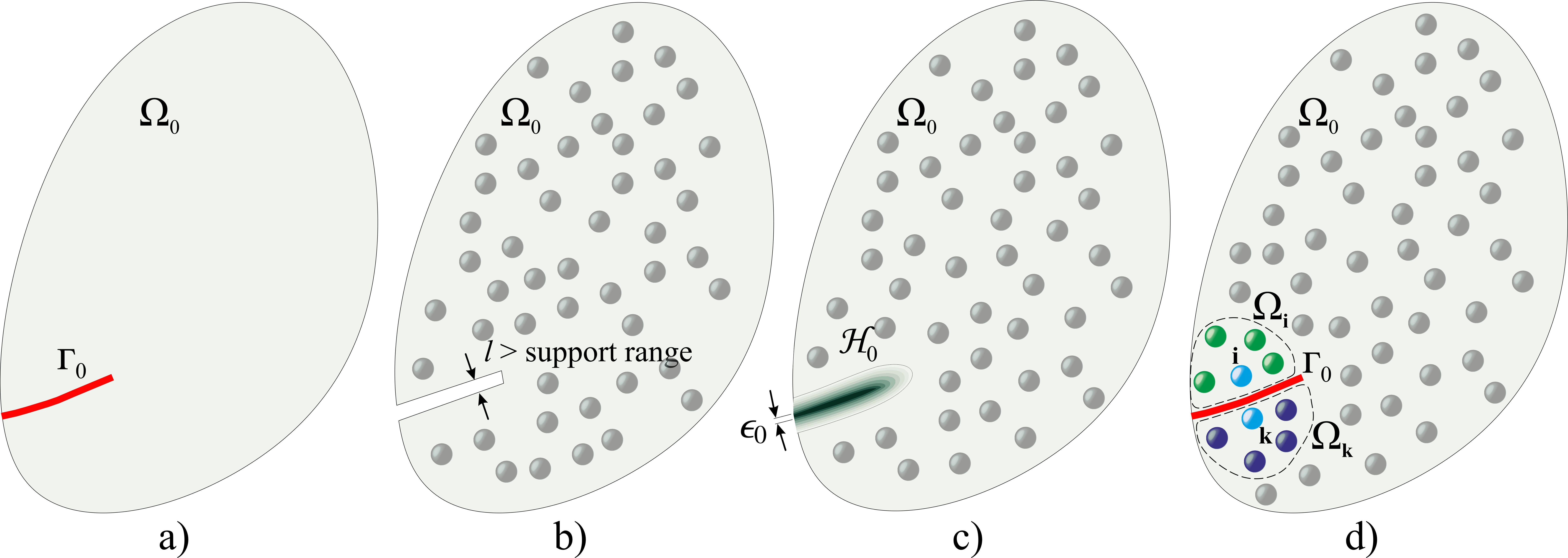
Figure 4: A description of a) preexisting discontinuity and its approximation by means of b) introducing a geometrical notch, c) assigning a prescribed value in the history functional, and d) restricting the neighbor search only among particles that lie in the same side of the discontinuity with the particle under consideration.

When it comes to time integration, a second-order Euler predictor-corrector time integration scheme is adopted with a CFL condition of

$$\Delta t\leq\text{min}\left(0.25\frac{h}{c_{0}+|\textbf{v}_{max}|},\,\frac{\Delta x}{c_{0}}\right),$$ (67)

where the second term ensures the stability of the phase field solution, and $\textbf{v}_{max}$ is the maximum possible velocity of the computational domain in space and time. At the beginning of each time step the field variables are updated utilizing the predictor scheme as

$$\mathbf{v}_{\mathbf{i}}^{(t+1/2)}=\mathbf{v}_{\mathbf{i}}^{(t)}+0.5\Delta t\left(\frac{d\mathbf{v}_{\textbf{i}}}{dt}\right)^{(t-1/2)}\text{,}$$ (68)

$$\mathbf{u}_{\mathbf{i}}^{(t+1/2)}=\mathbf{u}_{\mathbf{i}}^{(t)}+0.5\Delta t\mathbf{v}_{\mathbf{i}}^{(t+1/2)}\text{,}$$ (69)

$$\dot{s}_{\mathbf{i}}^{(t+1/2)}=\dot{s}_{\mathbf{i}}^{(t)}+0.5\Delta t\ddot{s}_{\textbf{i}}^{(t-1/2)}\text{,}$$ (70)

$$s_{\mathbf{i}}^{(t+1/2)}=s_{\mathbf{i}}^{(t)}+0.5\Delta t\dot{s}_{\mathbf{i}}^{(t+1/2)}\text{,}$$ (71)

where the superscripts $(t+1/2)$, $(t-1/2)$, and $(t)$ denote the values of the related field variable at half time step, previous half time step, and previous time step, respectively. Then, using the values of $\mathbf{u}^{(t+1/2)}$, the deformation gradient of the TLSPH particles is computed using Eqs.(61-62). At this stage, an appropriate constitutive model is utilized (see Section 4.2.1 or Section 4.2.2) to compute the first Piola–Kirchhoff stress tensor as a function of the computed deformation gradient and the predicted half time step values of phase field (damage). Then, Eq.(17), Eq.(66), and Eq.(65) are in turn solved using the values of the variables at half-time step to compute the acceleration $(d\mathbf{v}/dt)^{(t+1/2)}$, Laplacian of the phase field $(\nabla^{2}s)^{(t+1/2)}$, and the phase field inertia $\ddot{s}^{(t+1/2)}$, respectively. Finally, the corrected values for the field variables are computed as

$$\mathbf{v}_{\mathbf{i}}^{(t+1)}=\mathbf{v}_{\mathbf{i}}^{(t)}+\Delta t\left(\frac{d\mathbf{v}_{\textbf{i}}}{dt}\right)^{(t+1/2)}\text{,}$$ (72)

$$\mathbf{u}_{\mathbf{i}}^{(t+1)}=\mathbf{u}_{\mathbf{i}}^{(t)}+\Delta t\mathbf{v}_{\mathbf{i}}^{(t+1)}\text{,}$$ (73)

$$\dot{s}_{\mathbf{i}}^{(t+1)}=\dot{s}_{\mathbf{i}}^{(t)}+\Delta t\ddot{s}_{\textbf{i}}^{(t+1/2)}\text{,}$$ (74)

$$s_{\mathbf{i}}^{(t+1)}=s_{\mathbf{i}}^{(t)}+\Delta t\dot{s}_{\mathbf{i}}^{(t+1)}\text{,}$$ (75)

where the $(t+1)$ superscript denotes the current time step. Note that the initial conditions for $\dot{s}$ and $\ddot{s}$ are set to zero. Algorithm 2 and Algorithm 3 present the implementation of the time integration module and the constitutive models for a single step calculation, respectively. It should be noted that for problems involving the contact of two separate bodies an additional interface force is included in the momentum equation (Eq.(17)). Hence, the momentum equation becomes

Algorithm 2 Single step calculations of time integration module

1:

2:Time integration

3:

4:$\vartriangleright$ Apply dynamic force and/or displacement boundary conditions

5:

6:for i $\leftarrow$ 1 to Total number of particles do

7: $\vartriangleright$ Compute half-time step values of field variables using Eqs.(68-71)

8:end for

9:

10:for i $\leftarrow$ 1 to Total number of particles do

11: $\vartriangleright$ Compute deformation gradient $\textbf{F}_{\textbf{i}}$ as in Eq.(61), using half step displacement values

12: $\vartriangleright$ Utilize Algorithm 3 to calculate $\textbf{P}_{\textbf{i}}$, $\psi_{e\textbf{i}}^{+}$, and $\psi_{e\textbf{i}}^{-}$ using the appropriate constitutive model

13: if $\psi_{e\textbf{i}}^{+}>\mathcal{H}_{\textbf{i}}$ then

14:  $\vartriangleright$ $\mathcal{H}_{\textbf{i}}=\psi_{e\textbf{i}}^{+}$ (here we update the history functional)

15: end if

16: $\vartriangleright$ Compute $M_{\textbf{i}}$ parameter as in Eq.(36)  (note that we use the upper bound value of M)

17: $\vartriangleright$ Using half-step values of the phase field parameter $s^{(t+1/2)}$ compute the Laplacian $\nabla^{2}s_{\textbf{i}}$ as in Eq.(66)

18: $\vartriangleright$ Using half step values of $s^{(t+1/2)}$ and $\dot{s}^{(t+1/2)}$ compute $\ddot{s}^{(t+1/2)}$ as in Eq.(65)

19: $\vartriangleright$ If contact exists, using half-step values of $\textbf{x}^{(t+1/2)}$, compute contact force for particle i as in A

20:end for

21:

22:for i $\leftarrow$ 1 to Total number of particles do

23: $\vartriangleright$ Using half step values of field variables compute acceleration $(d\mathbf{v}_{\textbf{i}}/dt)^{(t+1/2)}$ as in Eq.(17) (or Eq.(76) for problems involving contact interactions)

24: $\vartriangleright$ Correct field variables using Eqs.(72-75)

25:end for

26:

27:$\vartriangleright$ Write results (occasionally)

Algorithm 3 Implementation of the Saint-Venant Kirchhoff and neo-Hookean hyperelastic constitutive models

1:

2:If constitutive model is Saint-Venant Kirchhoff:

3: $\vartriangleright$ Compute Green–Lagrange strain tensor as $E_{\mathbf{i}}^{ks}=\frac{1}{2}\left(F_{\mathbf{i}}^{mk}F_{\mathbf{i}}^{ms}+\delta^{ks}\right)$ (summation is done over index m)

4: $\vartriangleright$ Decompose $\textbf{E}_{\textbf{i}}$ into $\textbf{E}_{\textbf{i}}^{+}$ and $\textbf{E}_{\textbf{i}}^{-}$ using Eqs.(41-42)

5: $\vartriangleright$ Compute $\psi_{e\textbf{i}}^{+}$ and $\psi_{e\textbf{i}}^{-}$ using Eqs.(39-40)

6: $\vartriangleright$ Compute $\textbf{S}_{\textbf{i}}^{+}$ and $\textbf{S}_{\textbf{i}}^{-}$ using Eq.(45)

7: $\vartriangleright$ Compute $\textbf{S}_{\textbf{i}}=\left(s_{\textbf{i}}^{(t+1/2)}\right)^{2}\textbf{S}_{\textbf{i}}^{+}+\textbf{S}_{\textbf{i}}^{-}$

8: $\vartriangleright$ Compute $P^{ks}_{\textbf{i}}=F^{km}_{\textbf{i}}S^{ms}_{\textbf{i}}$ (summation is done over index m)

9:

10:Else if constitutive model is neo-Hookean:

11: $\vartriangleright$ Compute $J$, b, and $\overline{\textbf{b}}$ using Eq.(52), Eq.(53), and Eq.(54), respectively.

12: $\vartriangleright$ Compute $U(J)$ and $\overline{\psi}_{e}(\overline{\textbf{b}})$ using Eq.(50) and Eq.(51), respectively.

13: $\vartriangleright$ Compute $\psi_{e\textbf{i}}^{+}$ and $\psi_{e\textbf{i}}^{-}$ using Eq.(48) and Eq.(49), respectively.

14: $\vartriangleright$ Compute $\textbf{S}_{\textbf{i}}$ from Eq.(60) using half-step values of phase field, $s_{\textbf{i}}^{(t+1/2)}$.

15: $\vartriangleright$ Compute $P^{ks}_{\textbf{i}}=F^{km}_{\textbf{i}}S^{ms}_{\textbf{i}}$ (summation is done over index m)

16:

17:Else:

18: $\vartriangleright$ Apply a different constitutive model here to calculate $\textbf{P}_{\textbf{i}}$, $\psi_{e\textbf{i}}^{+}$, and $\psi_{e\textbf{i}}^{-}$

$$\frac{dv^{k}_{\textbf{i}}}{dt}=\sum_{\textbf{j}=1}^{N_{\textbf{i}}}m_{0\textbf{j}}\left(\frac{P^{ks}_{\textbf{i}}}{\rho^{2}_{0\textbf{i}}}+\frac{P^{ks}_{\textbf{j}}}{\rho^{2}_{0\textbf{j}}}+P^{ks}_{v\textbf{ij}}\right)~{}\frac{\partial W_{0\textbf{ij}}}{\partial X_{\textbf{j}}^{s}}+b_{0\textbf{i}}^{k}+\sum_{\textbf{a}=1}^{\hat{N}_{\textbf{i}}}f_{\textbf{ai}}r_{\textbf{ai}}^{k}~{}$$ (76)

where $\hat{N}_{\textbf{i}}$ is the total number of particles located at a separate body within the contact distance, $r_{c}$, of particle i, $r_{\textbf{ai}}^{k}$ is the k component of the relative position vector $\textbf{r}_{\textbf{ai}}=\textbf{x}_{\textbf{a}}-\textbf{x}_{\textbf{i}}$ between particles a and i calculated using the Eulerian coordinates x, as given in Fig. 5, and $f_{\textbf{ai}}$ is a scalar multiplier whose details are given in A. For the cases involving contact interaction in this paper we set $r_{c}=2.5\Delta x$ unless stated otherwise.

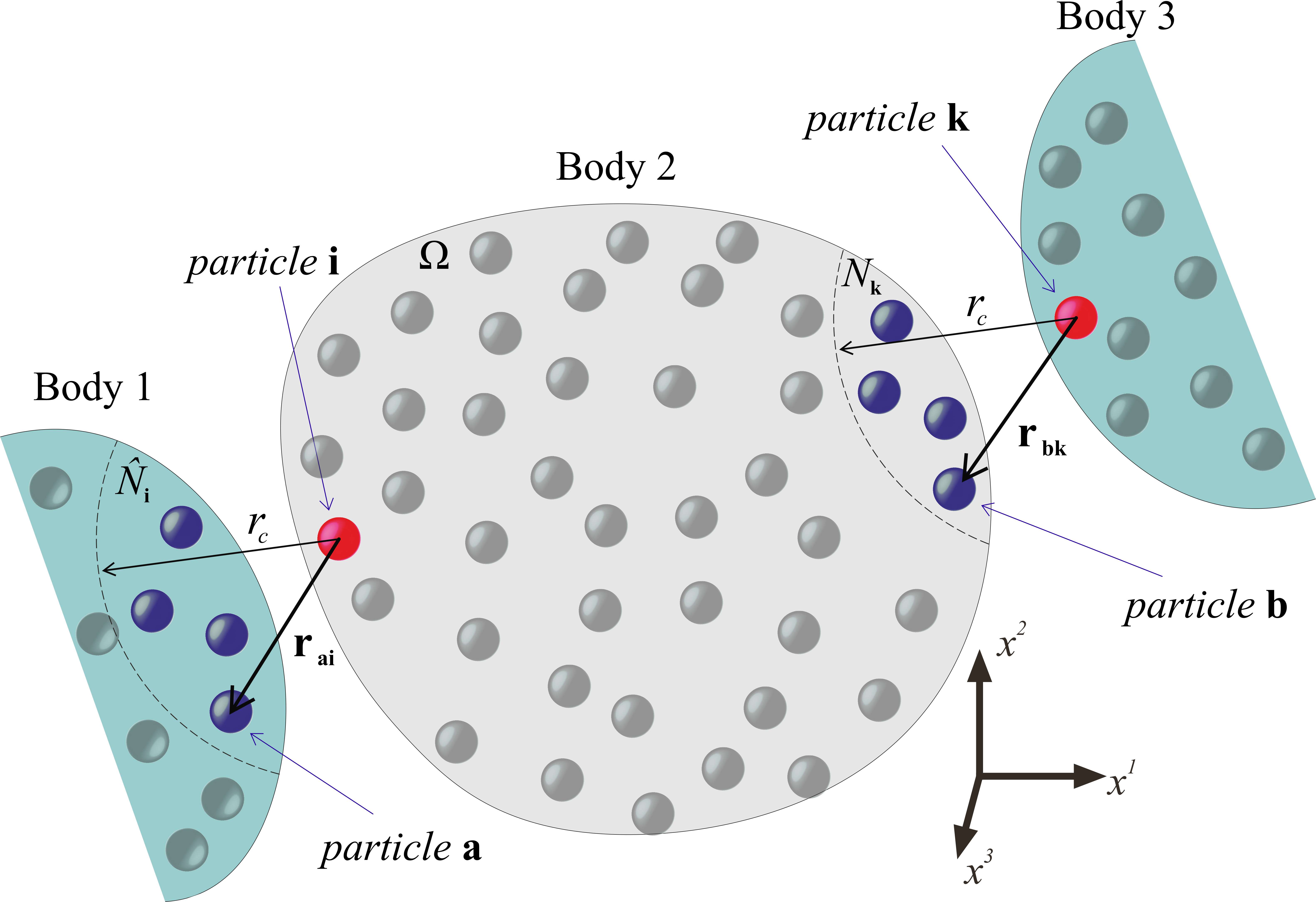
Figure 5: Interface details of the contact domain with multiple body contacts in SPH.

5 Numerical examples

In this section, we first apply the proposed framework to model various challenging problems from the literature. We then illustrate further capabilities of our model by addressing the failure occurrences in a three dimensional impact problem. All problems except the last one are simulated in two dimensions under plane strain assumption with a CPU parallel code. The simulations were carried out on a 40-core node on SeaWulf cluster located at the Institute for Advanced Computational Science (IACS) at Stony Brook University. The animated videos of the simulations are provided in Electronic Annex I (B).

5.1 Symmetric three point bending test

We first solve the crack propagation in a plate subjected to symmetric three point bending [27, 25]. The length and width of the plate are set to $L_{x}=8.2$ mm and $L_{y}=2$ mm, respectively. The material parameters $\lambda=12$ GPa, $\mu=8$ GPa, density $\rho_{0}=1190$ kg/m³, and $G_{c}=0.54$ kJ/m² are adopted from [25]. The contact parameters, length scale, and time step values, are set to $K_{p}=9\times 10^{12}$ and $r_{0}=2.5\Delta x$, $\epsilon_{0}=\Delta x$, and $\Delta t=0.1$ ns, respectively. A preexisting crack with a length of $0.4$ mm is located at the lower central portion of the plate and is modeled by restricting the neighbor search of the particles around the discontinuity region, as suggested in Section 4.3 and Fig. 4d. We enforce the boundary conditions through contact with rigid circular bands with outer diameters of $0.4$ mm at three regions, as shown in Fig. 6. The contact force is applied in the $X^{2}$-direction only, and a velocity of $-5$ m/s in the $X^{2}$-direction is assigned to the upper band, whereas the two lower bands are fixed in the $X^{1}$- and $X^{2}$-directions.

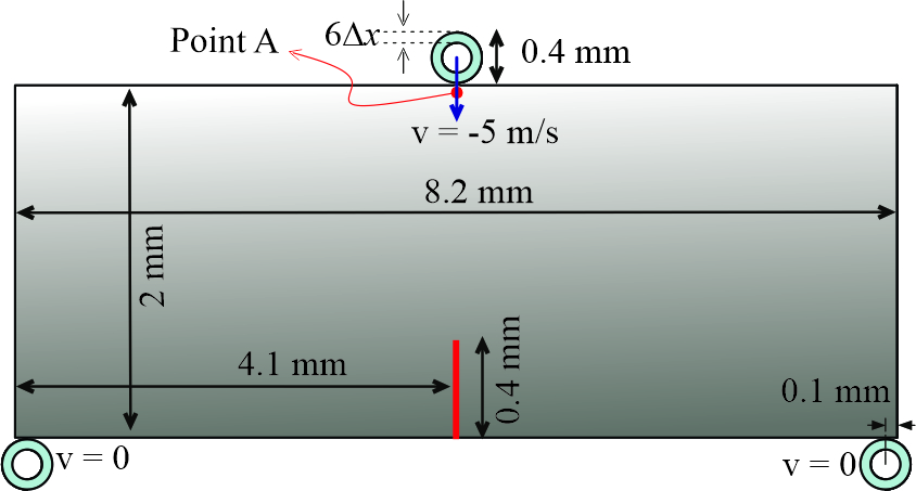
Figure 6: Symmetric three point bending test. Geometry and loading conditions.

We set the artificial viscosity parameters (see Section 2.3) to $\beta_{1}=0.2$ and $\beta_{2}=0$, and a phase field limit of $s_{l}=0.1$ is chosen for soft particles. The domain is discretized into $423,665$ particles with a particle spacing of $\Delta x=6.25$ $\mu$m, out of which $3,825$ particles belong to the contact bodies. Both the Saint-Venant Kirchhoff and Neo-Hookean constitutive models are employed. Fig. 7 shows the snapshots of the phase field parameter at different stages of the propagation.

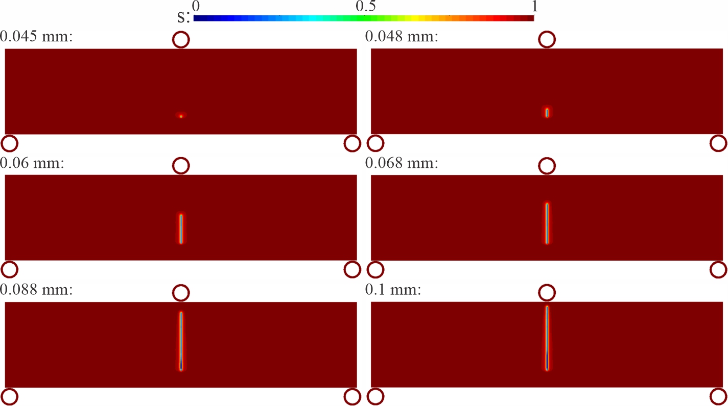
Figure 7: Symmetric three point bending test. Contours of the phase field parameter (crack path) for different values of the $X^{2}$-displacement of Point A. The snapshots correspond to computations performed with the Saint-Venant Kirchhoff constitutive model.

As can be seen, the propagation starts from the preexisting crack tip, continues in a vertical direction, and stops near the upper boundary of the plate. The start and end time of the propagation correspond to a displacement of $0.045$ mm and $0.1$ mm of Point A (see Fig. 6) in the $X^{2}$-direction, which agrees well with the ones reported in [25]. In Fig. 8 we compare the propagation length predicted by Saint-Venant Kirchhoff and Neo-Hookean constitutive models, in which both models deliver similar propagation curves.

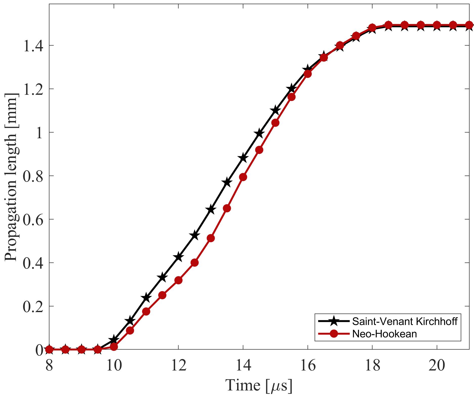
Figure 8: Symmetric three point bending test. Evolution of the propagation length of the crack for the Saint-Venant Kirchhoff and Neo-Hookean constitutive models.

5.2 Asymmetric three point bending test

Here, we model the asymmetric three point bending test [64, 27, 25]. The boundary conditions are similar to the previous case and are given in Fig. 9. The geometric properties and material parameters are adopted as $L_{x}=20$ mm, $L_{y}=8$ mm, $\lambda=12$ GPa, $\mu=8$ GPa, $\rho_{0}=1190$ kg/m³, and $G_{c}=1$ kJ/m².

Figure 9: Asymmetric three point bending test. Geometry and loading conditions.

We model the preexisting crack by restricting the neighbor search of the particles around the discontinuity region. The contact force is applied in the $X^{2}$-direction with contact parameters of $K_{p}=12\times 10^{12}$ and $r_{0}=2.5\Delta x$. Other simulation parameters are set to $\epsilon_{0}=\Delta x$, $\Delta t=0.1~{}ns$, $\beta_{1}=0.2$, $\beta_{2}=0$, and $s_{l}=0.1$. We discretize the domain into approximately 400K particles with a particle spacing of $\Delta x=0.02$ mm. The Saint-Venant Kirchhoff constitutive model is employed. Fig. 10 shows the snapshots of the phase field for the deformed plate at different stages of the propagation.

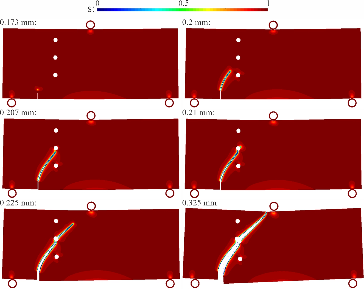
Figure 10: Asymmetric three point bending test. Contours of the phase field parameter (crack path) for different values of the $X^{2}$-displacement of Point A.

As can be seen, the crack initiation occurs when point A has displaced by approximately $0.17$ mm in the $X^{2}$-direction. Then, the crack joins the middle hole after a displacement of approximately $0.21$ mm, and the complete rupture is recorded at a displacement of around $0.325$ mm. The crack first propagates on a somewhat curved path from the preexisting crack tip to the middle hole, and then on an almost linear path until the full rupture. Fig. 11 compares the experimentally [64] and numerically [27, 25] obtained crack paths with the one predicted by the present approach.

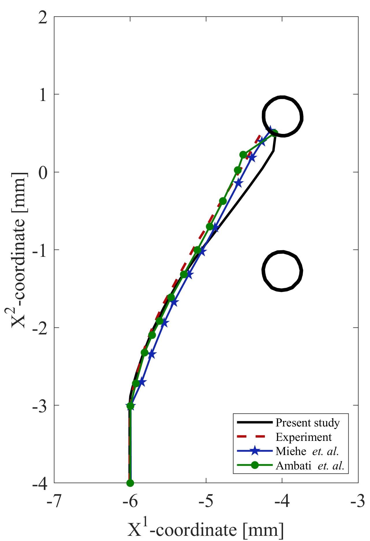
Figure 11: Asymmetric three point bending test. Crack path compared with experimental [64] and phase field results of Miehe et al. [25] and Ambati et al. [27].

As can be seen, the predicted crack path agrees very well with both the experimental and numerical studies found in the literature. There is a small deviation observed within a small region near the middle hole. One potential reason for this could be the imperfect representation of the circular holes in the discretized particle domain, which can alter the local strain energy concentrations. Nevertheless, the recorded deviation is negligible and does not change the overall physical behavior of the crack.

5.3 Dynamic crack branching

The dynamic crack branching problem has been widely investigated for different boundary conditions and loading setups [26, 58, 42, 65, 66]. In the present effort we focus on the setup used in [26, 58, 42], where a plate with a notch is subjected to a tensile surface loading. We set the material properties of the plate to $E=32$ GPa, $\rho=2450$ kg/m³, $\nu=0.2$, and $G_{c}=3$ J/m², whereas the Saint-Venant Kirchhoff constitutive model is employed. The length and width of the plate are taken as $L_{x}=100$ mm and $L_{y}=40$ mm, respectively. The preexisting notch is introduced as a geometrical discontinuity with a width of $4\Delta x$ and length of $50$ mm located at the center. The plate is assumed to be under a tensile load of $1$ MPa applied to its upper and lower surfaces, as depicted in Fig. 12. The length scale and time step values are set to $\epsilon_{0}=0.09375$ mm and $\Delta t=2.5$ ns, respectively. We set the artificial viscosity parameters (see Section 2.3) to $\beta_{1}=0.04$ and $\beta_{2}=0$, and a phase field limit of $s_{l}=0.1$ is chosen for soft particles.

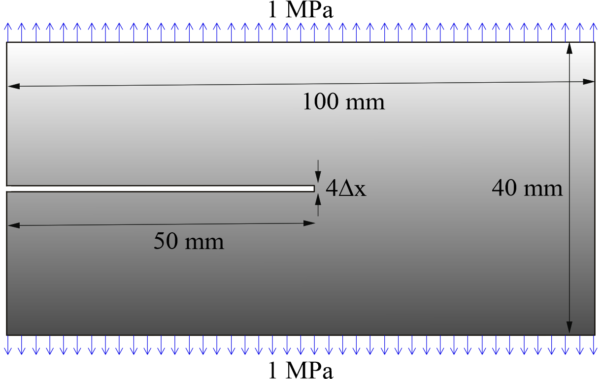
Figure 12: Dynamic crack branching. Geometry and loading conditions.

To demonstrate the resolution independence of the crack pattern in the phase field method, we consider four different particle resolutions, R1-R4, with initial particle spacing of $\Delta x=0.1$ mm, $\Delta x=0.08$ mm, $\Delta x=0.0625$ mm, and $\Delta x=0.05$ mm, leading to a discretization of the domain into $398,000$, $622,500$, $1,020,800$, and $1,596,000$ particles, respectively.

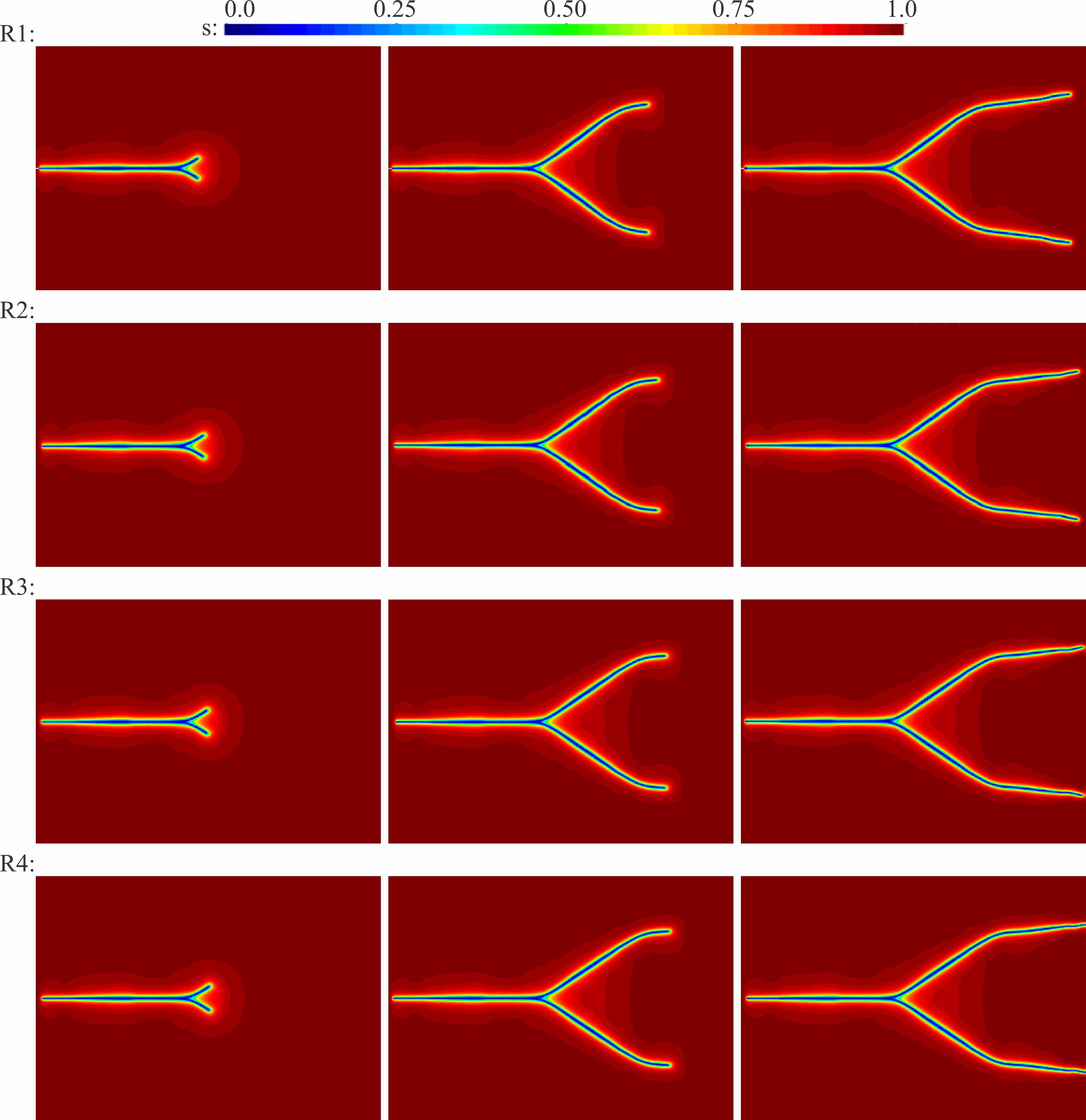
Figure 13: Dynamic crack branching. Contours of the phase field parameter (crack path) at $55~{}\mu$s (left), $80~{}\mu$s (middle), and $105~{}\mu$s (right), for R1-R4 resolutions. The snapshots are presented for the right half of the plate.

Fig. 13 presents several snapshots of the phase field contours for R1-R4 resolutions at different stages of the crack propagation for the right half of the plate (the left half stays intact and we therefore omit that region). The crack propagation starts from the tip of the notch at approximately $t=10$ $\mu$s and continues in a horizontal manner. At approximately $t=50$ $\mu$s, branching occurs, and the fracture propagates at an angle of $\approx 37^{o}$. At later stages, the propagation angles of the two branches tend to change back to horizontal. As expected, an identical crack pattern is predicted for all different resolutions, highlighting phase field’s feature of mesh independence, which is hard to achieve when local damage models are employed. At the same time, the predicted crack patterns are in excellent agreement with the ones reported in [26, 58, 42]. However, the crack in resolutions R1 and R2 fails to reach the end of the plate in the given time. This is a common behavior seen for low discretization resolutions and it is attributed to the fact that for lower resolutions the fracture zone is slightly wider and hence there is more fracture energy per unit length. Similar behavior was also reported in [26, 58, 42]. Fig. 14 compares the crack propagation speed predicted by the current model with the ones of [26, 58]. A close agreement is observed between the present results and the ones of [58]. In [26], however, a slightly higher propagation speed is reported. This difference is attributed to the absence of the inertia term ($\ddot{s}$) in the phase-field PDE utilized in [26] (see Section 3). Obviously, the inclusion of the inertia term in the current effort (i.e. the use of a hyperbolic phase field PDE instead of an elliptic one, as described in Section 3) introduces an extra amount of work to be carried out in order for the phase field to propagate, thereby causing a decrease in the propagation speed. However, it should be pointed out that no experimental data exist for this problem, therefore it is not clear which model’s crack propagation speed is more accurate. Nonetheless, as mentioned in [58], the elliptic models tend to overestimate the crack propagation speeds because they ignore the rate toughening effect in brittle fracture.

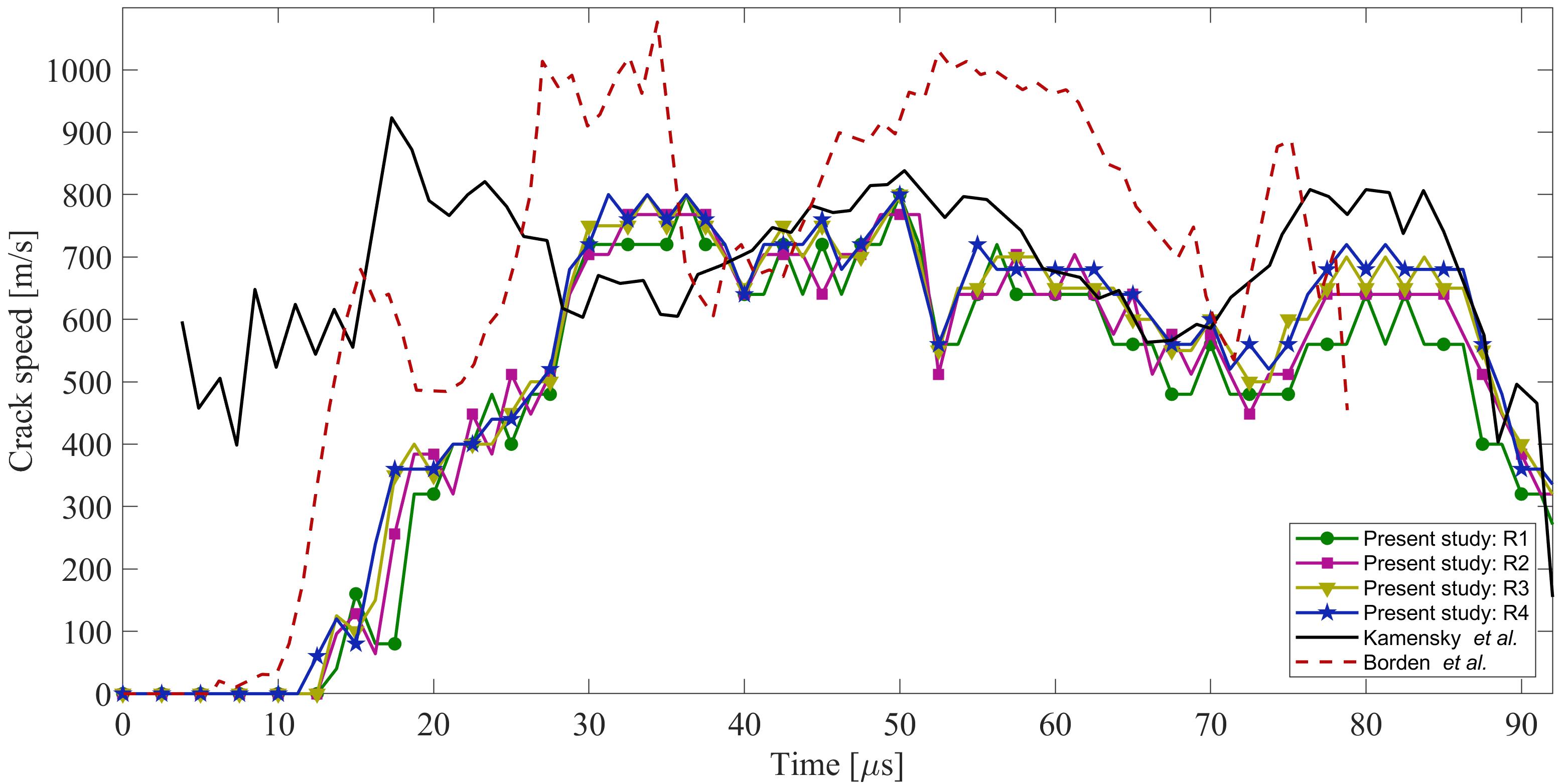
Figure 14: Dynamic crack branching. $X^{1}$- component of crack velocity for resolutions R1-R4 compared with the phase field results of Kamensky et al. [58] and Borden et al. [26].

It is also worth mentioning that the strategy employed to track the crack tip, and hence the propagation speed, highly affects the recorded crack initiation time. Here, we consider the furthest particle in the $+X^{1}$-direction with a phase field value of $s<0.7$ to be the tip of the crack. Therefore, as soon as the phase field value decreases to 0.7, the propagation is assumed to initiate. However, the choice of this value does not affect the computed propagation speed since the speed is computed between the two iso-curves of the same value.

In Fig. 15 the post-processed final results of the phase field and the crack opening are given for resolution R4, where the particles with $s<s_{l}=0.1$ are not shown, and the deformation is scaled by a factor of 50. As can be seen, after the complete failure, the domain separates into three regions, marking the end of the propagation.

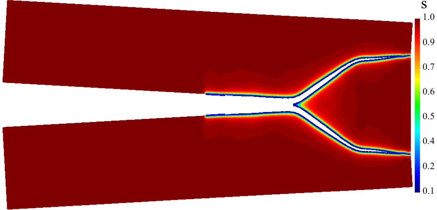
Figure 15: Dynamic crack branching. Opening of the crack and phase field distribution at the failure moment ($\approx 105$ $\mu$s) for resolution R4. Particles with $s<s_{l}=0.1$ are not shown. The deformation is magnified by a factor of $50$.

5.4 Kalthoff–Winkler experiment

Here we revisit the well-known Kalthoff–Winkler experiment where a plate is subjected to an impact shear loading [67]. The length and width of the plate are adopted from [26, 58, 42] as $L_{x}=100$ mm and $L_{y}=100$ mm, respectively. The material properties are set to $E=190$ GPa, $\rho=8000$ kg/m³, $\nu=0.3$, $G_{c}=22.13$ kJ/m², and the Saint-Venant Kirchhoff constitutive model is employed. The domain is discretized into $638,400$ particles with an initial particle spacing of $\Delta x=0.125$ mm. The length scale, time step, artificial viscosity parameters, and phase field limit for the soft particles, are chosen as $\epsilon_{0}=0.125$ mm, $\Delta t=1.0$ ns, $\beta_{1}=0.04$ and $\beta_{2}=0$, and $s_{l}=0.1$, respectively. A geometrical discontinuity with a width of $4\Delta x$ and length of $50$ mm is introduced in the left side of the plate to model the preexisting notch, as shown in Fig. 16.

Figure 16: Kalthoff–Winkler experiment. Geometry and loading conditions.

The plate is subjected to an impact loading in the horizontal direction, applied to the particles located at the lower portion of the left surface. The loading condition is applied as a time-dependent ramp-up velocity of

$$v=\left\{\begin{array}[]{lr}\frac{t}{t_{0}}16.5~{}m/s&t\leq t_{0}\\ 16.5~{}m/s&\text{otherwise}\end{array}\right.\text{ ,}$$ (77)

in the $X^{1}$-direction, where $t_{0}=1$ $\mu$s is the ramp-up time. Upon impact ($t=0$), the displacement field starts propagating towards the right, eventually causing stress and strain energy concentrations at the notch tip, which are then dissipated by the propagating crack (or phase field). Fig. 17 shows the snapshots of the results for different stages of the propagation. The crack propagation starts at approximately $25$ $\mu$s and continues diagonally until the full rapture at approximately $100$ $\mu$s. A local disturbance in the diagonal path of the crack is recorded between $t\approx 63$ $\mu$s and $t\approx 75$ $\mu$s (marked in Circle A in Fig. 17) which implies a mixed mode I–II fracture (also reported in [26, 58, 42]).

(a)

(b)

Figure 17: Kalthoff–Winkler experiment. a) Contours of the phase field parameter and b) opening of the crack at $50$ $\mu$s (left), $80$ $\mu$s (middle), and $101$ $\mu$s (right). In b), particles with $s<s_{l}=0.1$ are not shown and the deformation is magnified by a factor of $5$.

Fig. 18 compares the propagation speed and crack orientation predicted by the current approach with the ones of the elliptic phase field [26] and peridynamic [68] models. Due to the explicit dynamics nature of the present computations that results in a somewhat oscillatory behavior, the graphs were smoothed for visualization purposes. The portion belonging to the disturbance region (Circle A) is marked with gray color.

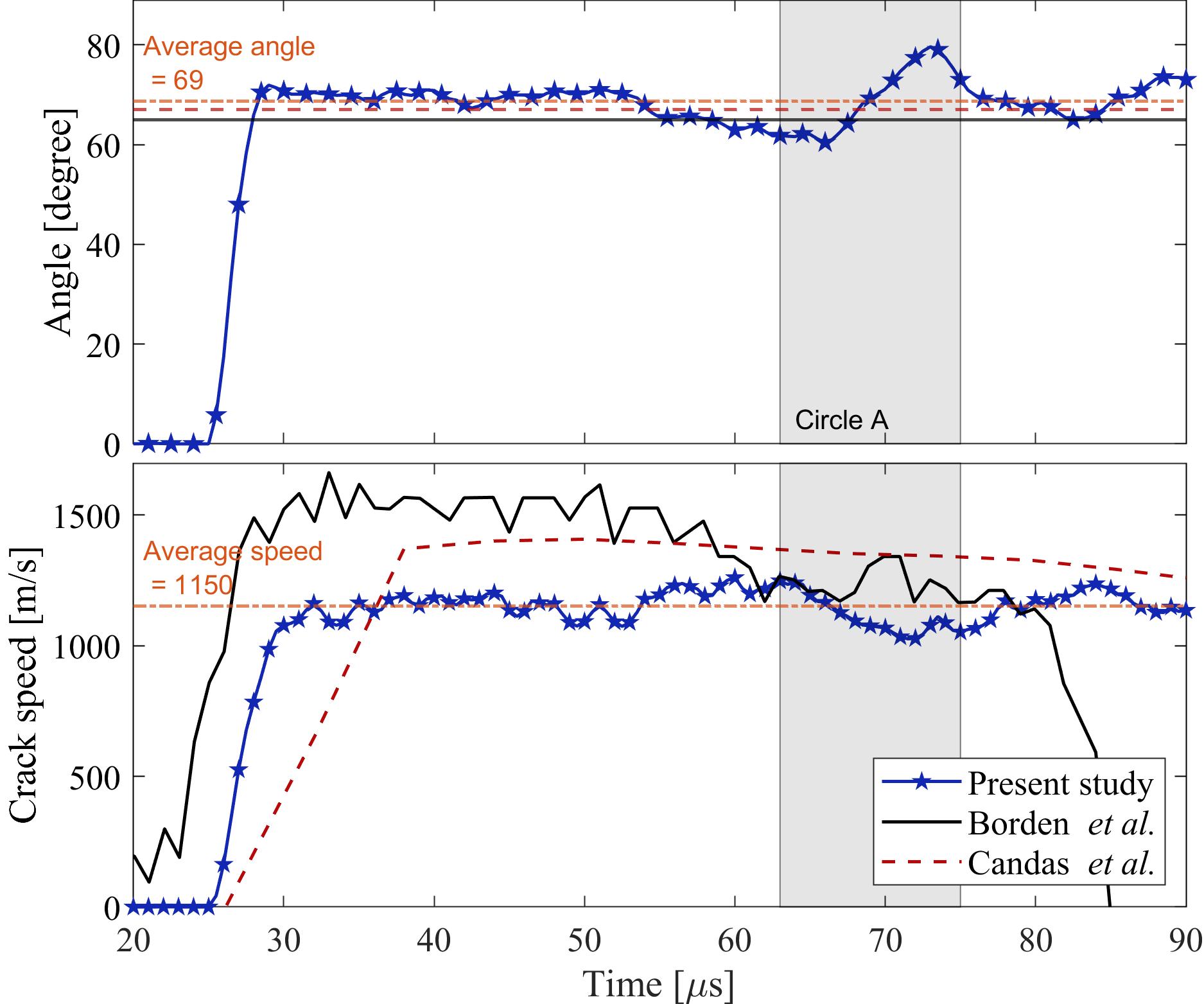
Figure 18: Kalthoff–Winkler experiment. Propagation speed and orientation of crack compared to phase field results of Borden et al. [26] and peridynamics results of Candas et al. [68].

The predicted results of crack propagation and orientation, as well as the elastodynamic behavior of the plate, are in good agreement with the aforementioned computational efforts and the corresponding experimental work. Overall, the proposed framework is able to capture all the complex qualitative and quantitative characteristics of the crack propagation.

5.5 Notched plate with hole

In this example, we simulate the interaction of cracks with other structural defects in a porous plate with an eccentric hole. The geometry of the plate is provided in Fig. 19. The material properties are set to $\lambda=1.94$ GPa, $\mu=2.45$ GPa, $\rho=2000$ kg/m³, $G_{c}=2.28$ kJ/m², and the Saint-Venant Kirchhoff constitutive model is employed. The domain is discretized into $732,852$ particles with an initial particle spacing of $\Delta x=0.1$ mm. The length scale, time step, artificial viscosity parameters, and phase field limit for the soft particles, are chosen as $\epsilon_{0}=0.1$ mm, $\Delta t=4.0$ ns, $\beta_{1}=0.04$ and $\beta_{2}=0$, and $s_{l}=0.1$, respectively.

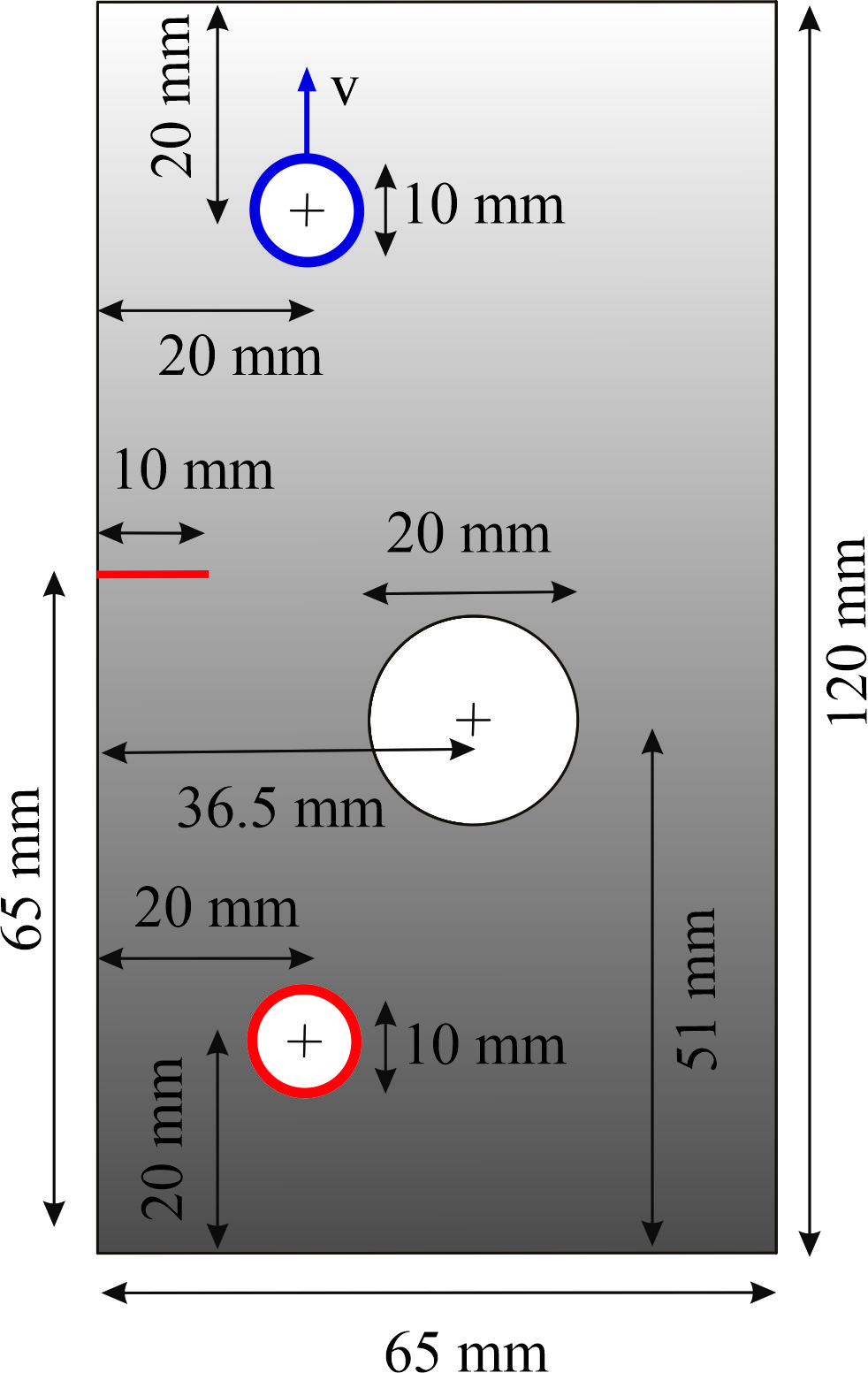
Figure 19: Notched plate with hole. Geometry and loading conditions. The particles around the lower hole (colored in red) are fixed in the $X^{1}$- and $X^{2}$-directions, and the prescribed velocity condition is applied to the particles around the upper hole (colored in blue) in the $X^{2}-$direction. The preexisting crack with a length of $10$ mm can be seen in red $65$ mm from the bottom edge of the specimen.

The original experiment [27] was performed in a displacement-control manner, where a prescribed displacement rate of $0.1$ mm/min was applied. The corresponding simulations [27, 69, 29] were carried out under static displacement loading condition. For both the experiment and the simulations, the prescribed displacement was applied to the upper hole (colored in blue in Fig. 19) of the plate, while the lower hole (colored in red in Fig. 19) was fixed in the horizontal and vertical directions. Here, due to the explicit nature of the SPH method, we conduct dynamic simulations, with three different cases of prescribed velocity in the vertical direction; $v=0.5$ m/s, $0.2$ m/s, $0.1$ m/s, applied on two layers of particles around the upper hole, whereas the two layers of particles around the lower hole are fixed in the $X^{1}$- and $X^{2}$-directions. A preexisting crack with a length of $10$ mm is located in the left-central portion of the plate, as shown in Fig. 19, and is modeled by restricting the neighbor search of the particles around the discontinuity region, as suggested in Section 4.3 and Fig. 4d.

The crack initiation is observed after the upper hole has displaced by approximately $0.3$ mm in the $X^{2}$-direction for all three cases of the prescribed velocity. The presence of the eccentric hole forms a weak-zone in the vicinity of the crack tip which generates the so-called accelerating effect on the propagating crack [70, 65]. As a result, the crack path is directed towards the hole, and eventually joins the hole after a displacement of approximately $0.4$ mm. Upon joining the hole the crack dissipates its energy, leading to a significant delay in propagation, caused by the arresting effect of the hole. At a displacement of approximately $1.4$ mm, a new crack initiates from the right side of the hole and causes a fast and complete rapture. The complex physics in terms of the accelerating and arresting effects of the hole on the crack are well-captured by the proposed approach. Identical accelerating and arresting effects were reported in [70, 65] using peridynamics. Fig. 20 depicts the snapshots of the final crack pattern under different prescribed velocity loading conditions.

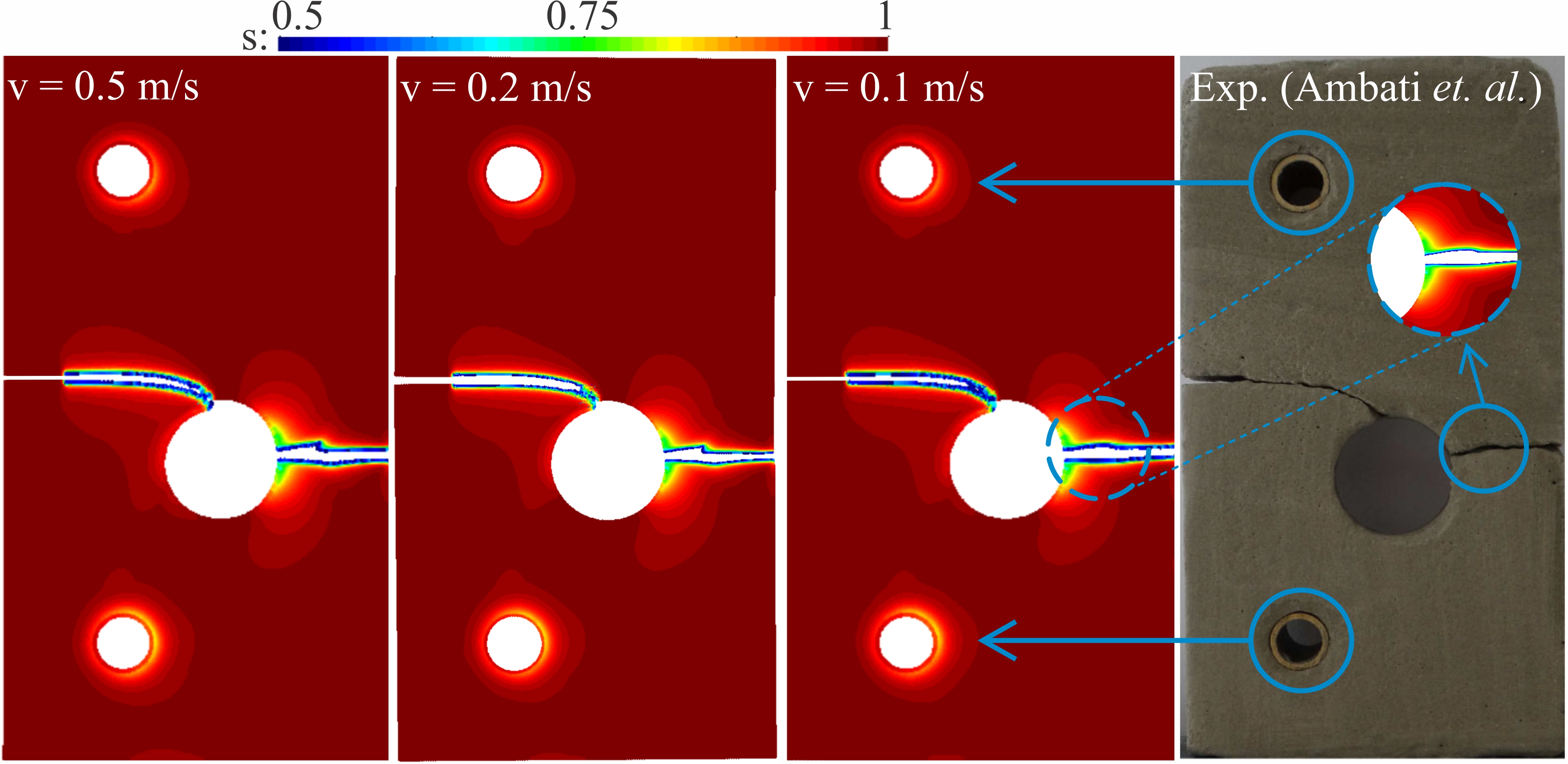
Figure 20: Notched plate with hole. Comparison of the final crack path with the experimental results of Ambati et al. [27]. Particles with $s<0.5$ are not shown.

As it is seen, the present approach is able to capture all the major qualitative features of fracture, such as the damaged region around the supports, as well as the tendency of the crack to branch in the vicinity of the eccentric hole (marked with circles in Fig. 20), which demonstrates a good agreement with the experimental results of [27]. A small deviation of the crack path in terms of small branching is observed for higher prescribed velocity values. This is in agreement with the reported effects of the dynamic loading on crack branching [71] and the experimental observations in [27]. Fig. 21 compares the phase field values for different loading conditions at various stages of the propagation. As can be seen, for lower values of the prescribed velocity, the branching effect close to the hole vanishes, which agrees well with the findings of [71].

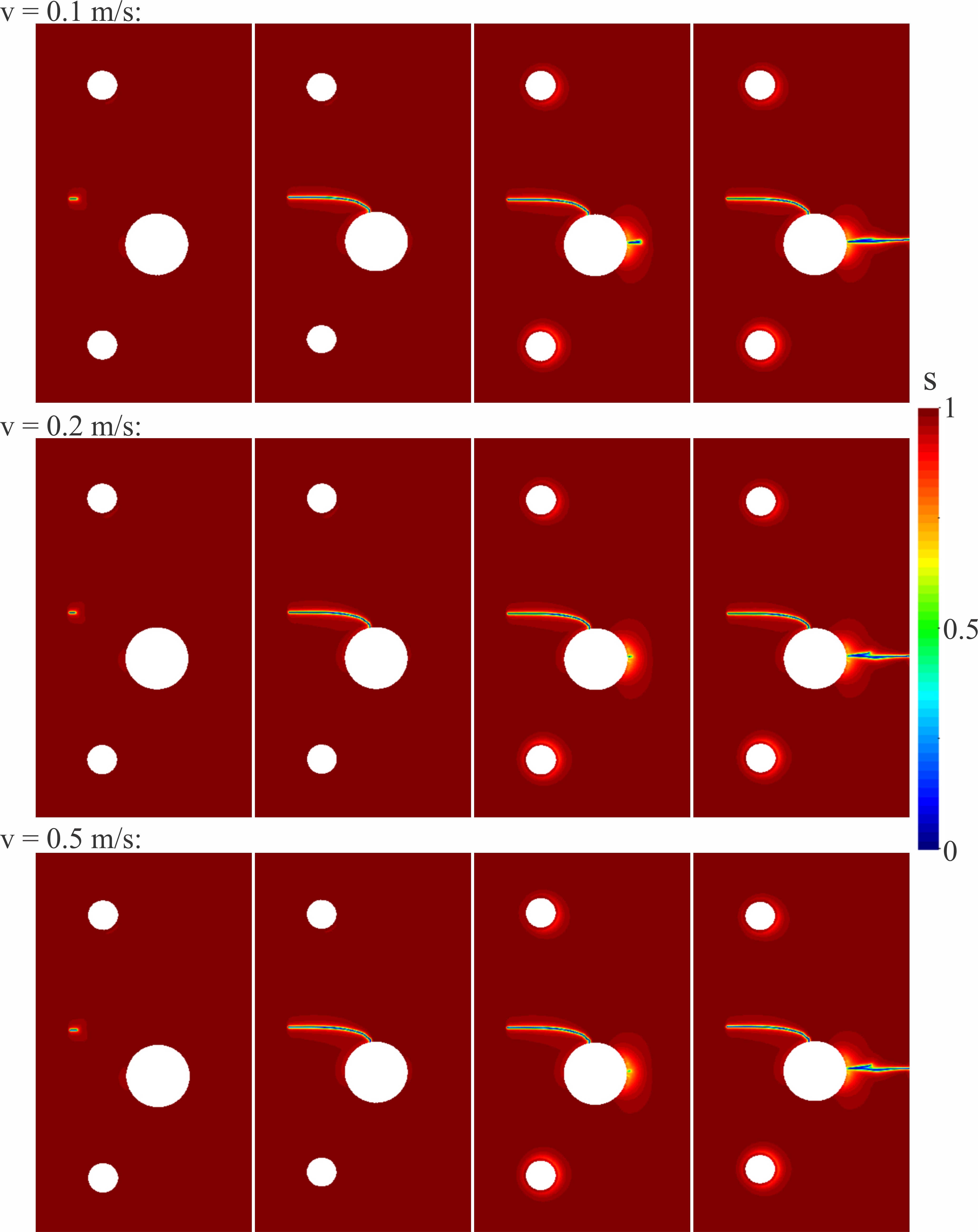
Figure 21: Notched plate with hole. Contours of the phase field parameter (crack path) under different velocity loading conditions for upper hole displacement values of $0.3$ mm (first column), $0.42$ mm (second column), $1.42$ mm (third column), and $1.48$ mm (fourth column).

Fig. 22 presents the smoothed graph of the reaction force (at the lower hole) versus maximum displacement (displacement of the upper hole) for $v=0.1$ m/s.

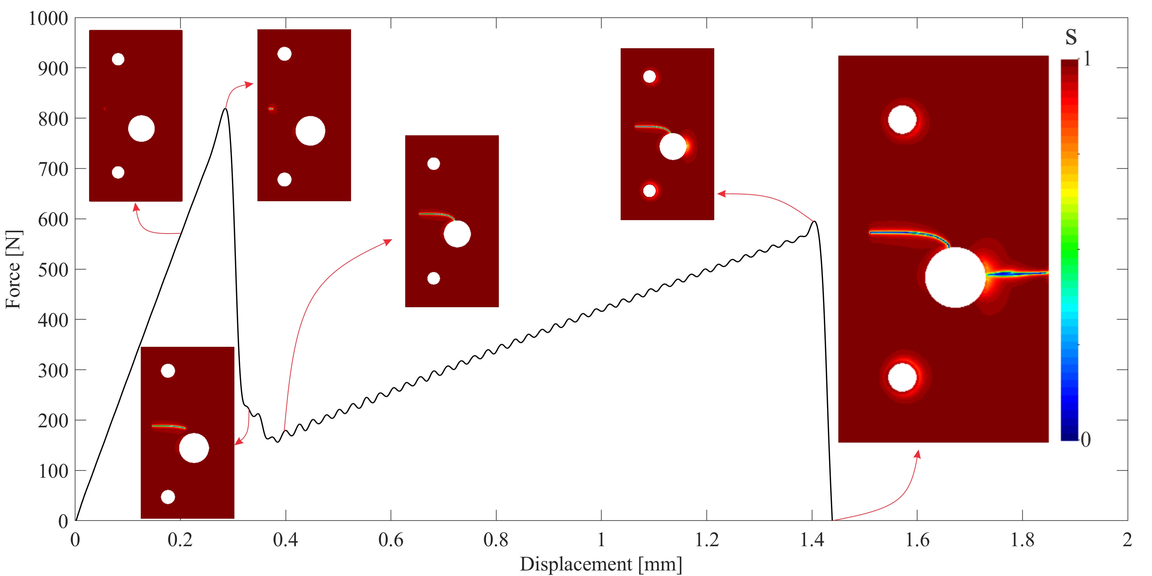
Figure 22: Notched plate with hole. Reaction force–displacement graph for $v=0.1$ m/s. Snapshots of the crack at various stages are superimposed for a comparative view.

We would like to point out that although this problem has been investigated by several researchers in the past [27, 69, 29], the corresponding reaction force–displacement graphs are not in agreement among each other. Furthermore, all the previous works, in contrast to the present effort, solved the problem in a static manner. Hence, some discrepancies are expected in the reaction force–displacement curve. However, the qualitative features of the graph are captured well. Moreover, the time at which the first crack initiation occurs (sudden drop in the curve at approximately $0.3$ mm) is in excellent agreement with the one reported in [69, 29].

5.6 Impact of a spherical projectile on a notched circular plate

To further demonstrate the capabilities of our proposed framework we simulate the impact of a rigid spherical projectile on a notched circular plate. Fig. 23 illustrates the geometric properties of the domain in which the diameter and thickness of the plate are given as $37$ mm and $5\Delta x$, respectively.

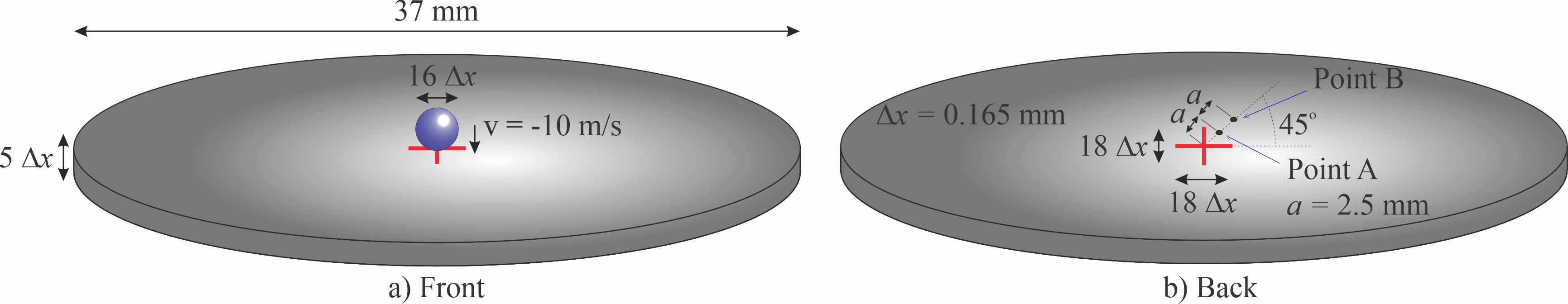
Figure 23: Impact of a spherical projectile on a notched circular plate. Geometry and loading conditions.

A rigid spherical projectile with a diameter of $16\Delta x$ and a prescribed velocity of $-10$ m/s in the $X^{3}$-direction impacts the plate at time $t=0$. A through-the-thickness cross-shaped notch with side lengths of $18\Delta x$ is applied at the center of the plate and is modeled by restricting the neighbor search of the particles around the notch. The displacement is constrained at the outer edge of the plate. We set the material and simulation parameters to $\lambda=4.75$ GPa, $\mu=0.9$ GPa, $\rho_{0}=1200$ kg/m³, $G_{c}=703$ J/m², $\epsilon_{0}=\Delta x$, $\Delta t=2.5$ ns, $\beta_{1}=0.05$, $\beta_{2}=0$, $s_{l}=0.1$, $r_{0}=2\Delta x$, and $K_{p}=1.2\times 10^{12}$. The domain is discretized into $800,774$ particles and the particle spacing is $\Delta x=0.165$ mm, whereas the Neo-Hookean constitutive model is employed. Fig. 24 and Fig. 25 show the three- and two- dimensional views of the phase field in the deformed plate, respectively.

Figure 24: Impact of a spherical projectile on a notched circular plate. Three dimensional view of the phase field parameter.

Figure 25: Impact of a spherical projectile on a notched circular plate. Two dimensional view of the phase field parameter.

As can be seen, upon impact the plate starts to deform, and after approximately $80$ $\mu$s the propagation initiates from the back side of the preexisting notch tips. Since the back side of the plate undergoes higher tension than the front, the propagation at the back starts earlier. At later stages of the propagation, the plate is forced to break from the boundaries of the weak regions under high tension which correspond to the regions under the impact of the projectile, thus, leading to an ultimate penetration. After the penetration, the plate bounces back and dissipates its accumulated strain energy marking the end of crack propagation. Fig. 26 shows the displacements of Point A and Point B (see Fig. 23) in the $X^{3}$-direction with respect to time.

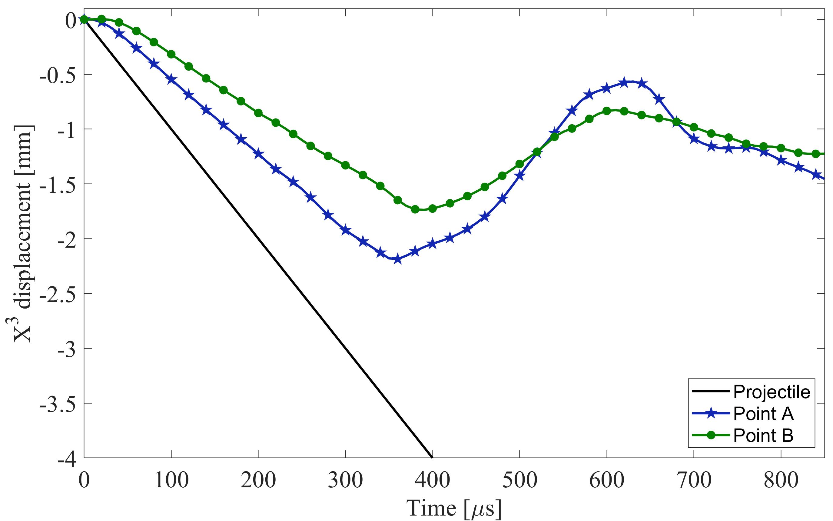
Figure 26: Impact of a spherical projectile on a notched circular plate. Displacements of Point A and Point B in the $X^{3}$-direction.

As can be seen, the proposed approach is able to efficiently capture the pre- and post-failure behaviors of the complex contact problem with complex fracture patterns. This problem is merely a demonstration of capabilities, and although neither experimental nor numerical results exist for comparison purposes, all the qualitative features that are expected from the underlying physics are produced.

6 Conclusions

We presented a robust, accurate, and convergent computational framework for modeling dynamic brittle fracture within the SPH method. The proposed approach employs the well-known SPH approximation technique to discretize a coupled system of a recently developed hyperbolic phase field model of brittle fracture and solid mechanics. The use of SPH allows for the simulation of large deformation problems that potentially involve multi-body interactions and fragmentation, whereas the use of a hyperbolic PDE for the phase field governing equation permits explicit integration in time, without having to solve expensive linear systems associated with elliptic models, or introduce severe time step restrictions associated with parabolic models.

The results of fracture simulations performed with the proposed formulation are in excellent agreement with solutions calculated using standard mesh-based numerical techniques, such as the finite element method and isogeometric analysis. At the same time, they are in very good agreement with results from experimental studies. The last numerical example, although it does not have any corresponding experimental or numerical results, is a demonstration-of-capabilities study, and produces all the qualitative features that are expected from the underlying physics.

This proof-of-concept work presents the core formulation for coupling solid mechanics with phase field for fracture within the SPH framework. Immediate future efforts will focus on large deformation fluid–structure interaction problems, functionally graded materials, as well as parallelization based on graphics processing units (GPU).

Appendix A Interface force for contact problems in SPH

In a typical contact problem in SPH an additional term arising from the contact of two separate bodies is included in the governing equation. Thus, the resulting momentum equation (Eq.(17)) becomes

$$\frac{dv^{k}_{\textbf{i}}}{dt}=\sum_{\textbf{j}=1}^{N_{\textbf{i}}}m_{0\textbf{j}}\left(\frac{P^{ks}_{\textbf{i}}}{\rho^{2}_{0\textbf{i}}}+\frac{P^{ks}_{\textbf{j}}}{\rho^{2}_{0\textbf{j}}}+P^{ks}_{v\textbf{ij}}\right)~{}\frac{\partial W_{0\textbf{ij}}}{\partial X_{\textbf{j}}^{s}}+b_{0\textbf{i}}^{k}+\sum_{\textbf{a}=1}^{\hat{N}_{\textbf{i}}}f_{\textbf{ai}}r_{\textbf{ai}}^{k}~{}.$$ (78)

In the newly included term, $\hat{N}_{\textbf{i}}$ is the total number of particles located at a separate body within the contact distance of particle i, $r_{\textbf{ai}}^{k}$ is the k component of the relative position vector $\textbf{r}_{\textbf{ai}}=\textbf{x}_{\textbf{a}}-\textbf{x}_{\textbf{i}}$ between particles a and i calculated using the Eulerian coordinates x (see Fig. 5), and $f_{\textbf{ai}}$ is a scalar multiplier. Borrowing mostly from [72] we calculate $f_{\textbf{ai}}$ as

$$f_{\textbf{ai}}=\frac{m_{0\textbf{a}}K_{p}}{|\textbf{r}_{\textbf{ai}}|^{2}}\left\{\begin{array}[]{lr}B_{\textbf{ai}}R_{\textbf{ai}}&|\textbf{r}_{\textbf{ai}}|\leq r_{c}\\ \textbf{0}&\text{otherwise}\end{array}\right.\text{~{}}{,}$$ (79)

where

$$B_{\textbf{ai}}=\frac{1+\frac{|\textbf{r}_{\textbf{ai}}|}{r_{c}}}{1-e}\left(e^{1+\frac{|\textbf{r}_{\textbf{ai}}|}{r_{c}}}-1\right)\text{~{}}{,}$$ (80)

$$R_{\textbf{ai}}=\left\{\begin{array}[]{lr}\frac{(1+1.5\tilde{q})(2-\tilde{q})^{3}}{8}&\frac{d(|\textbf{r}_{\textbf{ai}}|)}{dt}\leq 0\\ 0&\text{otherwise}\end{array}\right.\text{~{}}{,}$$ (81)

$$\tilde{q}=\frac{|\textbf{r}_{\textbf{ai}}|}{1.33\Delta x}\text{~{}}{.}$$ (82)

$m_{0\textbf{a}}$ is the initial mass of particle a, $r_{c}$ is the contact distance, and $K_{p}$ is a constant determining the potential of the contact. The $K_{p}$ and $r_{c}$ constants need to be determined carefully through numerical experiments in order to preserve the physical nature of contact and to avoid any penetration.

Appendix B Supplementary data

Supplementary material related to this article can be found online at https://doi.org/10.1016/j.cma.2022.115191.

References

- [1] Robert A. Gingold and Joseph J. Monaghan. Smoothed particle hydrodynamics: theory and application to non-spherical stars. Monthly Notices of the Royal Astronomical Society, 181(3):375–389, 1977.
- [2] Leon. B. Lucy. A numerical approach to the testing of the fission hypothesis. The Astronomical Journal, 82(12):1013–1024, 1977.
- [3] Joseph J. Monaghan. Simulating free surface flows with sph. Journal of Computational Physics, 110(2):399–406, 1994.
- [4] Larry Libersky and Albert Petschek. Smooth particle hydrodynamics with strength of materials’, in Advances in the Free-Lagrange Method, volume 395, pages 248–257. 01 2006.
- [5] Jeff W. Swelge, Darrell L. Hicks, and Steve W. Attaway. SPH Stability Analysis. Journal of Computational Physics, 116:123–134, 1995.
- [6] Carl T. Dyka and Robert P. Ingel. An approach for tension instability in smoothed particle hydrodynamics (sph). Computers & Structures, 57(4):573–580, 1995.
- [7] Javier Bonet and T. S.L. Lok. Variational and momentum preservation aspects of Smooth Particle Hydrodynamic formulations. Computer Methods in Applied Mechanics and Engineering, 180(1-2):97–115, 1999.
- [8] Joseph J. Monaghan. Smoothed particle hydrodynamics. Reports on Progress in Physics, 68(8):1703–1759, 2005.
- [9] Juan R. Reveles. Development of a total Lagrangian SPH code for the simulation of solids under dynamic loading. PhD thesis, Cranfield University, 2007.
- [10] M.B. Liu and G.R. Liu. Smoothed Particle Hydrodynamics (SPH): an Overview and Recent Developments. Archives of Computational Methods in Engineering, 17(1):25–76, 2010.
- [11] Leonardo Di G. Sigalotti, Jaime Klapp, Otto Rendón, Carlos A. Vargas, and Franklin Peña-Polo. On the kernel and particle consistency in smoothed particle hydrodynamics. Applied Numerical Mathematics, 108:242–255, 2016.
- [12] Shan Qun Chen, Bin Liao, and Tao Huang. Corrected SPH methods for solving shallow-water equations. Journal of Hydrodynamics, 28(3):389–399, 2016.
- [13] M. Naqib Rahimi, Deniz Can Kolukisa, Mehmet Yildiz, Murat Ozbulut, and Adnan Kefal. A generalized hybrid smoothed particle hydrodynamics–peridynamics algorithm with a novel lagrangian mapping for solution and failure analysis of fluid–structure interaction problems. Computer Methods in Applied Mechanics and Engineering, 389:114370, 2022.
- [14] Timon Rabczuk and J Eibl. Simulation of high velocity concrete fragmentation using sph/mlsph. International Journal for Numerical Methods in Engineering, 56(10):1421–1444, 2003.
- [15] Timon Rabczuk and Ted Belytschko. Cracking particles: a simplified meshfree method for arbitrary evolving cracks. International Journal for Numerical Methods in Engineering, 61(13):2316–2343, 2004.
- [16] Nicolas Moës, John Dolbow, and Ted Belytschko. A finite element method for crack growth without remeshing. International Journal for Numerical Methods in Engineering, 46(1):131–150, 1999.
- [17] Nicolas Moës and Ted Belytschko. Extended finite element method for cohesive crack growth. Engineering Fracture Mechanics, 69(7):813–833, 2002.
- [18] Sukanta Chakraborty and Amit Shaw. A pseudo-spring based fracture model for sph simulation of impact dynamics. International Journal of Impact Engineering, 58:84–95, 2013.
- [19] Md Rushdie Ibne Islam and Chong Peng. A total lagrangian sph method for modelling damage and failure in solids. International Journal of Mechanical Sciences, 157:498–511, 2019.
- [20] Md Rushdie Ibne Islam and Amit Shaw. Pseudo-spring sph simulations on the perforation of metal targets with different damage models. Engineering Analysis with Boundary Elements, 111:55–77, 2020.
- [21] Yingnan Wang, Ha H. Bui, Giang D. Nguyen, and PG Ranjith. A new sph-based continuum framework with an embedded fracture process zone for modelling rock fracture. International Journal of Solids and Structures, 159:40–57, 2019.
- [22] Yingnan Wang, Hieu T. Tran, Giang D. Nguyen, Pathegama G. Ranjith, and Ha H. Bui. Simulation of mixed-mode fracture using sph particles with an embedded fracture process zone. International Journal for Numerical and Analytical Methods in Geomechanics, 44(10):1417–1445, 2020.
- [23] Ha H. Bui and Giang D. Nguyen. Smoothed particle hydrodynamics (SPH) and its applications in geomechanics: From solid fracture to granular behaviour and multiphase flows in porous media. Computers and Geotechnics, 138:104315, 2021.
- [24] Charlotte Kuhn and Ralf Müller. A phase field model for fracture. In PAMM: Proceedings in Applied Mathematics and Mechanics, volume 8, pages 10223–10224. Wiley Online Library, 2008.
- [25] Christian Miehe, Martina Hofacker, and Fabian Welschinger. A phase field model for rate-independent crack propagation: Robust algorithmic implementation based on operator splits. Computer Methods in Applied Mechanics and Engineering, 199(45-48):2765–2778, 2010.
- [26] Michael J. Borden, Clemens V. Verhoosel, Michael A. Scott, Thomas J.R. Hughes, and Chad M. Landis. A phase-field description of dynamic brittle fracture. Computer Methods in Applied Mechanics and Engineering, 217-220:77–95, 2012.
- [27] Marreddy Ambati, Tymofiy Gerasimov, and Laura De Lorenzis. A review on phase-field models of brittle fracture and a new fast hybrid formulation. Computational Mechanics, 55(2):383–405, 2015.
- [28] Jian-Ying Wu and Vinh Phu Nguyen. A length scale insensitive phase-field damage model for brittle fracture. Journal of the Mechanics and Physics of Solids, 119:20–42, 2018.
- [29] Adrian Egger, Udit Pillai, Konstantinos Agathos, Emmanouil Kakouris, Eleni Chatzi, Ian A. Aschroft, and Savvas P. Triantafyllou. Discrete and phase field methods for linear elastic fracture mechanics: A comparative study and state-of-the-art review. Applied Sciences, 9(12), 2019.
- [30] Jian-Ying Wu, Vinh Phu Nguyen, Chi Thanh Nguyen, Danas Sutula, Sina Sinaie, and Stéphane PA Bordas. Phase-field modeling of fracture. In Advances in Applied Mechanics, volume 53, pages 1–183. Elsevier, 2020.
- [31] Lampros Svolos, Curt A Bronkhorst, and Haim Waisman. Thermal-conductivity degradation across cracks in coupled thermo-mechanical systems modeled by the phase-field fracture method. Journal of the Mechanics and Physics of Solids, 137:103861, 2020.
- [32] Tushar Kanti Mandal, Vinh Phu Nguyen, Jian-Ying Wu, Chi Nguyen-Thanh, and Alban de Vaucorbeil. Fracture of thermo-elastic solids: Phase-field modeling and new results with an efficient monolithic solver. Computer Methods in Applied Mechanics and Engineering, 376:113648, 2021.
- [33] Lampros Svolos, Hashem M Mourad, Curt A Bronkhorst, and Haim Waisman. Anisotropic thermal-conductivity degradation in the phase-field method accounting for crack directionality. Engineering Fracture Mechanics, 245:107554, 2021.
- [34] Gilles A Francfort and J-J Marigo. Revisiting brittle fracture as an energy minimization problem. Journal of the Mechanics and Physics of Solids, 46(8):1319–1342, 1998.
- [35] Blaise Bourdin, Gilles A Francfort, and Jean-Jacques Marigo. Numerical experiments in revisited brittle fracture. Journal of the Mechanics and Physics of Solids, 48(4):797–826, 2000.
- [36] Alan Arnold Griffith. Vi. the phenomena of rupture and flow in solids. Philosophical transactions of the royal society of London. Series A, containing papers of a mathematical or physical character, 221(582-593):163–198, 1921.
- [37] Michael J Borden, Thomas JR Hughes, Chad M Landis, and Clemens V Verhoosel. A higher-order phase-field model for brittle fracture: Formulation and analysis within the isogeometric analysis framework. Computer Methods in Applied Mechanics and Engineering, 273:100–118, 2014.
- [38] Lin Chen, Bin Li, and René de Borst. Adaptive isogeometric analysis for phase-field modeling of anisotropic brittle fracture. International Journal for Numerical Methods in Engineering, 121(20):4630–4648, 2020.
- [39] Khuong D Nguyen, Cuong-Le Thanh, H Nguyen-Xuan, and Magd Abdel-Wahab. A hybrid phase-field isogeometric analysis to crack propagation in porous functionally graded structures. Engineering with Computers, pages 1–21, 2021.
- [40] Fatemeh Amiri, Daniel Millán, Marino Arroyo, Mohammad Silani, and Timon Rabczuk. Fourth order phase-field model for local max-ent approximants applied to crack propagation. Computer Methods in Applied Mechanics and Engineering, 312:254–275, 2016.
- [41] Emmanouil G. Kakouris and Savvas P. Triantafyllou. Phase-field material point method for brittle fracture. International Journal for Numerical Methods in Engineering, 112(12):1750–1776, 2017.
- [42] Georgios Moutsanidis, David Kamensky, JS Chen, and Yuri Bazilevs. Hyperbolic phase field modeling of brittle fracture: Part II—immersed IGA–RKPM coupling for air-blast–structure interaction. Journal of the Mechanics and Physics of Solids, 121:114–132, 2018.
- [43] Emmanouil G. Kakouris and Savvas P. Triantafyllou. Phase-field material point method for dynamic brittle fracture with isotropic and anisotropic surface energy. Computer Methods in Applied Mechanics and Engineering, 357:112503, 2019.
- [44] Ngoc-Hien Nguyen, Vinh Phu Nguyen, Jian-Ying Wu, Thi-Hong-Hieu Le, Yan Ding, et al. Mesh-based and meshfree reduced order phase-field models for brittle fracture: One dimensional problems. Materials, 12(11):1858, 2019.
- [45] Yulong Shao, Qinglin Duan, and Shasha Qiu. Adaptive consistent element-free galerkin method for phase-field model of brittle fracture. Computational Mechanics, 64(3):741–767, 2019.
- [46] Weidong Li, Nhon Nguyen-Thanh, and Kun Zhou. Phase-field modeling of brittle fracture in a 3d polycrystalline material via an adaptive isogeometric-meshfree approach. International Journal for Numerical Methods in Engineering, 121(22):5042–5065, 2020.
- [47] Junchao Wu, Dongdong Wang, Zeng Lin, and Dongliang Qi. An efficient gradient smoothing meshfree formulation for the fourth-order phase field modeling of brittle fracture. Computational Particle Mechanics, 7(2):193–207, 2020.
- [48] Yulong Shao, Qinglin Duan, and Shasha Qiu. Adaptive analysis for phase-field model of brittle fracture of functionally graded materials. Engineering Fracture Mechanics, 251:107783, 2021.
- [49] Yury Krongauz and Ted Belytschko. Consistent pseudo-derivatives in meshless methods. Computer Methods in Applied Mechanics and Engineering, 146(3-4):371–386, 1997.
- [50] Jean Paul Vila. On particle weighted methods and smooth particle hydrodynamics. Mathematical Models and Methods in Applied Sciences, 9(2):161–209, 1999.
- [51] Ted Belytschko, Yong Guo, Wing Kam Liu, and Shao Ping Xiao. A unified stability analysis of meshless particle methods. International Journal for Numerical Methods in Engineering, 48(9):1359–1400, 2000.
- [52] Joseph Peter Morris. An overview of the method of smoothed particle hydrodynamics. 1995.
- [53] Timon Rabczuk, Ted Belytschko, and Shaoping Xiao. Stable particle methods based on Lagrangian kernels. Computer Methods in Applied Mechanics and Engineering, 193(12-14):1035–1063, 2004.
- [54] J.J. Monaghan. Particle methods for hydrodynamics. Computer Physics Reports, 3(2):71–124, 1985.
- [55] Jun Lin, Hakim Naceur, Daniel Coutellier, and Abdel Laksimi. Geometrically nonlinear analysis of two-dimensional structures using an improved smoothed particle hydrodynamics method. Engineering Computations, 32(3):779–805, jan 2015.
- [56] Jiandong He, Nima Tofighi, Mehmet Yildiz, Juanmian Lei, and Afzal Suleman. A coupled wc-tl sph method for simulation of hydroelastic problems. International Journal of Computational Fluid Dynamics, 31(3):174–187, 2017.
- [57] Joseph J. Monaghan and Robert A. Gingold. Shock simulation by the particle method sph. Journal of Computational Physics, 52(2):374–389, 1983.
- [58] David Kamensky, Georgios Moutsanidis, and Yuri Bazilevs. Hyperbolic phase field modeling of brittle fracture: Part I—Theory and simulations. Journal of the Mechanics and Physics of Solids, 121:81–98, 2018.
- [59] Andreas Peer, Christoph Gissler, Stefan Band, and Matthias Teschner. An implicit sph formulation for incompressible linearly elastic solids. In Computer Graphics Forum, volume 37, pages 135–148. Wiley Online Library, 2018.
- [60] Gerhard A Holzapfel. Nonlinear solid mechanics: a continuum approach for engineering science. Meccanica, 37(4):489–490, 2002.
- [61] Michael J. Borden, Thomas J.R. Hughes, Chad M. Landis, Amin Anvari, and Isaac J. Lee. A phase-field formulation for fracture in ductile materials: Finite deformation balance law derivation, plastic degradation, and stress triaxiality effects. Computer Methods in Applied Mechanics and Engineering, 312:130–166, 2016.
- [62] Joseph J. Monaghan. Smoothed particle hydrodynamics. Annual Review of Astronomy and Astrophysics, 30(1):543–574, 1992.
- [63] Leigh Brookshaw. A method of calculating radiative heat diffusion in particle simulations. Publications of the Astronomical Society of Australia, 6(2):207–210, January 1985.
- [64] Tulio N. Bittencourt, Paul A. Wawrzynek, Anthony R. Ingraffea, and J.L. Sousa. Quasi-automatic simulation of crack propagation for 2d lefm problems. Engineering Fracture Mechanics, 55(2):321–334, 1996.
- [65] M. Naqib Rahimi, Adnan Kefal, Mehmet Yildiz, and Erkan Oterkus. An ordinary state-based peridynamic model for toughness enhancement of brittle materials through drilling stop-holes. International Journal of Mechanical Sciences, 182(May), 2020.
- [66] M. Naqib Rahimi. Peridynamic modelling of internal features and interfaces for material toughening. Master’s thesis, Sabanci University, dec 2020.
- [67] J.F. Kalthoff and S. Winkler. Failure mode transition at high rates of shear loading. DGM Informationsgesellschaft mbH, Impact Loading and Dynamic Behavior of Materials, 1:185–195, 1988.
- [68] Adem Candaş, Erkan Oterkus, and Cevat Erdem İmrak. Dynamic Crack Propagation and Its Interaction With Micro-Cracks in an Impact Problem. Journal of Engineering Materials and Technology, 143(1), 08 2020.
- [69] Yousef Navidtehrani, Covadonga Betegón, and Emilio Martínez-Pañeda. A unified abaqus implementation of the phase field fracture method using only a user material subroutine. Materials, 14(8):1–19, 2021.
- [70] M. Naqib Rahimi, Adnan Kefal, and Mehmet Yildiz. An improved ordinary-state based peridynamic formulation for modeling FGMs with sharp interface transitions. International Journal of Mechanical Sciences, 197(December 2020):106322, 2021.
- [71] Florin Bobaru and Guanfeng Zhang. Why do cracks branch? A peridynamic investigation of dynamic brittle fracture. International Journal of Fracture, 196(1-2):59–98, 2015.
- [72] Rui Yan, Yong qiang Bi, and Wei Jiang. Simulation of contact interface between elastic solids using smoothed particle hydrodynamics. Computational Particle Mechanics, 9(1):167–177, 2022.