Complex structure and characterization
of multi-photon split states in integrated circuits

Abstract

Multi-photon split states, where each photon is in a different spatial mode, represent an essential resource for various quantum applications, yet their efficient characterization remains an open problem. Here, we formulate the general structure of their reduced spatial density matrices and identify the number of real and complex-valued independent coefficients, which in particular completely determine the distinguishability of all photons. Then, we show that this density matrix can be fully characterized by measuring correlations after photon interference in a static integrated circuit, where the required outputs scale sub-quadratically versus the number of photons. We present optimized circuit designs composed of segmented coupled waveguides, representing a linear optical neural network, which minimize the reconstruction error and facilitate robustness to fabrication deviations.

I Introduction

The multi-photon split states (M-PSS), where each photon is in a different spatial mode of free-space beams, fibers, or waveguides, represent an essential resource for fundamental tests of quantum mechanics and various applications in quantum simulations and computations [1]. For example, many photon interference and distinguishability experiments are based on M-PSSs where each photon is injected from a different spatial port [2, 3, 4, 5, 6, 7, 8]. Furthermore, photon boson sampling experiments that can demonstrating quantum advantage commonly employ PSS sources that provide multiple indistinguishable photons with each of the photons injected to a different port of a linear optical network [9, 10, 11, 12, 13, 14]. Remarkably, PSSs with more than two photons were recently shown to possess a multi-photon collective phase beyond the real-valued pair-wise photon distinguishability measure, opening new degrees of freedom for quantum information [4, 15, 16]. Therefore, the characterisation of PSSs is of great importance from fundamental and practical perspectives.

Importantly, the indistinguishability of all photons in M-PSS cannot be inferred from the distinguishability of constituent photon pairs, which demands the characterization based on multi-photon interference. Efficient protocols for witnessing multiphoton indistinguishability were developed and realized with reconfigurable multi-port interfrometers [7] under the assumption of a specific density matrix form, whereas this remains an open problem for general states (see a discussion in the Supplementary of Ref. [6]).

Beyond the quantification of indistinguishability, the measurement of the full density matrix can provide comprehensive information about the state, including the collective photon phase. This is typically done by a process called quantum state tomography, where the density matrix of the input quantum state is reconstructed after a series of projection measurements [17, 18, 19]. To fully reconstruct the density matrix, the number of distinct measurements which are in the form of multi-photon correlations should exceed the number of free parameters in the density matrix that increases exponentially with the number of photons [20]. To satisfy this requirement, conventional tomography approaches are based on free-space setups or integrated circuits that are reconfigured multiple times [21, 22, 7], yet the reconfiguration can be a source of experimental inaccuracies and also make the characterization time-consuming for larger numbers of photons. On the other hand, static tomography approaches have been suggested [23, 24, 25, 26, 27] and realized experimentally [28, 29], where the measurements at the outputs of a fixed photonic circuit enable the full state reconstruction. However, such methods have been developed for general states without taking into account the specific structure of PSSs. It remained an outstanding question of how to perform optimal characterization of PSSs with the minimum number of measurements, high robustness to fabrication inaccuracy, and measurement noise while using the most compact and practical photonic circuit design.

In this work, we formulate the general properties of the spatial density matrix structure for the PSSs without any assumptions. Then, we present a scalable approach for single-shot complete state measurement with a static integrated photonic circuit, without a need for reconfigurability. Specifically, we first theoretically derive the number of free parameters and the structure of the reduced spatial density matrix as a function of the number of photons. Furthermore, we obtain the number of free real and imaginary parts, in which the imaginary values of the density matrix are associated with the multi-photon collective phases. To realize the state tomography, we propose a multiport coupled waveguide array that is segmented into multiple sections along the propagation direction with the specially introduced local phase shifts between adjacent sections. Such a configuration effectively represents a photonic neural network (NN), where the waveguide coupling and local phase shifts function as the weight and bias, respectively. By optimizing the photonic circuit, we identify the configurations allowing for the most efficient tomography of two-, three- and four-photon split states with reduced sensitivity to measurement noise and fabrication deviations. Different from previous reconfigurable platforms which require multiple measurements with an exponential increase in the number of photons, the proposed scheme can realize the tomography in a single shot without reconfigurability. When compared with previous static approaches developed for general states, the performance is better and the complexity of the photonic circuit is reduced. This makes the proposed scheme scalable to larger photon numbers.

The paper is organized as follows. In Sec. II, we formulate the general structure of the reduced spatial density matrix for PSSs after tracing out the internal spectral degree of freedom and determine the numbers of independent real- and complex-valued coefficients as a function of the number of photons. In the following Sec. III, we introduce a circuit design based on coupled waveguides, representing a linear artificial neural network, and describe its application for split-state tomography. Then, in Sec. IV, we present the circuit designs for two-, three- and four-photon split states, optimized for accurate state reconstruction in presence of measurement noise or fabrication imperfections. Finally, we present conclusions and outlook in Sec. V

II Multi-photon split states and the spatial density matrix

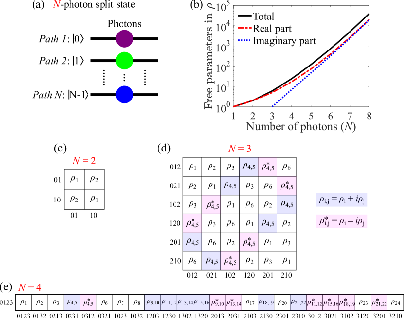
Figure 1: (a) Schematic of the $N$-photon split state (PSS) where each photon is located in a different spatial mode or path. (b) Number of real, imaginary, and total independent parameters in the reduced spatial density matrix of N-PSS as a function of the number of photons. (c,d) The structure of the reduced spatial density matrices for (b) two- and (c) three-PSSs. The elements without or with backgrounds are purely real or complex-valued, respectively. Note that only the nonzero elements of the full density matrix (dimension: $N^{N}\times N^{N}$) are shown. (e) First row of the nonzero elements of the four-PSS density matrix. Other rows will have the same elements in different orders.

We define a multi-photon split state formed by $N$ photons where each photon is located on a different spatial path with orthogonal states labeled by $|0\rangle$, $|1\rangle$, $\cdots$, $|N-1\rangle$, as shown in Fig. 1(a). The frequency dependent wavefunction of such a PSS can be expressed as

$$|\Psi\rangle=\int d\omega_{0}d\omega_{1}\cdots d\omega_{N-1}\psi(\omega_{0},\omega_{1},\cdots,\omega_{N-1})\hat{a}_{0}^{\dagger}(\omega_{0})\hat{a}_{1}^{\dagger}(\omega_{1})\cdots\hat{a}_{N-1}^{\dagger}(\omega_{N-1})|0\rangle,$$ (1)

where $\psi(\omega_{0},\omega_{1},\cdots,\omega_{N-1})$ is the joint spatial and spectral distribution of $N$ photons. Note that the $|0\rangle$ in Eq. (1) stands for the photon vacuum state instead of the spatial mode of the first path mentioned earlier.

We consider the setups using commonly available single-photon click detectors. The coincidences of signals from several detectors then provide a measure of the photon correlations. While the photons might have different internal structure, such as frequency spectra, the conventional detectors only register the arrival time within specific time bins. Such detection and correlation measurements in photonic circuits do not distinguish the photons by their spectral properties [22, 30]. Also, experiments can realize multi-photon interference that does not explicitly depend on the internal structure of photons [4, 28, 29, 16], and such transformations are mathematically described by a unitary operator that mixes different input ports but does not depend on frequency spectra of photons [31, 15]. In addition, the single-photon click detectors cannot resolve the number of photons that arrived on the detector.

For the case where the experimental detectors do not distinguish the photons by their spectrum, a PSS can be characterized by a reduced density matrix, where the internal spectrum degree of freedom of the photons is traced out via integration. In the reduced spatial density matrix, which has a dimension of $N^{N}\times N^{N}$, each element is determined by [28]:

$$\rho_{s^{\prime}_{0},s^{\prime}_{1},\cdots s^{\prime}_{N-1};s_{0},s_{1},\cdots s_{N-1}}={\rm Tr}\left(\hat{\rho}\,\hat{O}_{s^{\prime}_{0},s^{\prime}_{1},\cdots s^{\prime}_{N-1};s_{0},s_{1},\cdots s_{N-1}}\right)\,,$$ (2)

where $\hat{\rho}=|\Psi\rangle\langle\Psi|$ is the full density matrix, and the $N$-photon density matrix projection operator is defined as

$$\hat{O}_{s^{\prime}_{0},s^{\prime}_{1},\cdots s^{\prime}_{N-1};s_{0},s_{1},\cdots s_{N-1}}=\frac{1}{N!}\int d\omega_{0}d\omega_{1}\cdots d\omega_{N-1} {\hat{a}_{s^{\prime}_{0}}^{\dagger}(\omega_{0})\hat{a}_{s^{\prime}_{1}}^{\dagger}(\omega_{1})\cdots\hat{a}_{s^{\prime}_{N-1}}^{\dagger}(\omega_{N-1})|0\rangle}$$ (3)

$${\langle 0|\hat{a}_{s_{0}}(\omega_{0})\hat{a}_{s_{1}}(\omega_{1})\cdots\hat{a}_{s_{N-1}}(\omega_{N-1})}.$$

For a split state, the nonzero density matrix elements can only be associated with indices $(s^{\prime}_{0},s^{\prime}_{1},\cdots,s^{\prime}_{N-1})$ and $(s_{0},s_{1},\cdots,s_{N-1})$ that are permutations in the set $(0,1,\cdots,N-1)$ without repetitions. We also note that the reduced density matrix is invariant under the simultaneous exchange of indices $s^{\prime}_{i}\leftrightarrow s^{\prime}_{j}$ and $s_{i}\leftrightarrow s_{j}$ for arbitrary $i$ and $j$, since the photons are indistinguishable after the internal spectrum degree of freedom is traced out. Using this property, we can map all the elements to just the first row of the density matrix with elements $\rho_{0,1,\cdots,N-1,s_{0}s_{1}\cdots s_{N-1}}$, where $(s^{\prime}_{0},s^{\prime}_{1},\cdots,s^{\prime}_{N-1})=(0,1,\cdots,{N-1})$. Therefore, the number of nonzero and independent elements of the spatial density matrix is the number of permutations of $(s_{0},s_{1},\cdots,s_{N-1})$ in the set $(0,1,\cdots,N-1)$ without repetition, which is $N!$.

Within this formulation, we can associate the appearance of collective multi-photon phase [15] with the presence of complex-valued density matrix elements. Since the ordering of $|0\rangle\langle s_{0}|,|1\rangle\langle s_{1}|,\cdots,|N-1\rangle\langle s_{N-1}|$ doesn’t affect the values of density matrix elements, we have

$$\begin{split}\rho_{0,1,\cdots N-1;s_{0},s_{1},\cdots s_{N-1}}&=\rho_{q_{0},q_{1},\cdots q_{N-1};0,1,\cdots N-1}\\ &=\rho_{0,1,\cdots N-1;q_{0},q_{1},\cdots q_{N-1}}^{\ast},\end{split}$$ (4)

where $(s_{0},s_{1},\cdots s_{N-1})$ is reordered into $(0,1,\cdots N-1)$ and $(q_{0},q_{1},\cdots q_{N-1})$ is the new order from $(0,1,\cdots N-1)$ after the same permutation operation. When $(q_{0},q_{1},\cdots q_{N-1})\equiv(s_{0},s_{1},\cdots s_{N-1})$, then it follows from Eq. (4) that $\rho_{0,1,\cdots,N-1;s_{0},s_{1},\cdots,s_{N-1}}=\rho_{0,1,\cdots,N-1;s_{0},s_{1},\cdots,s_{N-1}}^{\ast}$, i.e. this element is real-valued. Let us denote the number of such cases by $A_{N}$. The remaining $N!-A_{N}$ elements will have complex values and include $(N!-A_{N})/2$ complex-conjugate pairs. Correspondingly, the number of independent real and imaginary parts of the density matrix are $(N!+A_{N})/2$ and $(N!-A_{N})/2$, respectively, resulting in a total of $N!$ real-valued free parameters. We prove that $A_{N}$ satisfies the recurrence relation $A_{N}=A_{N-1}+(N-1)A_{N-2}$ for $N\geq 3$, with $A_{1}=1$ and $A_{2}=2$, see Appendix A for the derivation.

We show in Fig. 1(b) the number of total, real, and imaginary independent parameters of the split-state density matrix as a function of the number of photons. For $N=(2,3,4)$, there are $(2,6,24)$ total, $(2,5,17)$ real, and $(0,1,7)$ imaginary parameters. The corresponding structures of the reduced density matrices are presented in Figs. 1(c-e). We label the independent real and imaginary coefficients with single sequential indices. The Figs. 1(c) and 1(d) illustrate that one row contains all the different elements, and we show just the first row for four-PSS in Figs. 1(e) to save space. Notably, the imaginary parts can only appear for three or more photons ($N\geq 3$), in agreement with the properties of collective multi-photon phase [4, 15, 16].

We emphasise that the number of independent density matrix parameters for split states ($N!$) is much smaller than that for the general states [28]. This allows for the efficient tomography of split states by taking into account their structure, as we discuss in the following.

III Integrated circuit for split-state measurements

We now analyse how the characterization of split states can be performed by adopting a static tomography approach [23, 24, 25, 26, 27, 28, 29]. We consider an $N$-input-$M$-output waveguide circuit where the $N$ input photons interfere, and the $N$-photon correlations are measured between different combinations of the $M$ output ports, as schematically shown in Fig. 2(a). To realise the state tomography without reconfigurability, the number of different $N$-photon correlation measurements at the output should exceed the number of unknown density matrix elements, that is

$$\frac{M!}{N!(M-N)!}\geq N!\,.$$ (5)

The required minimum number of waveguides $M$ grows linearly up to five-photon states, $M_{\rm min}=2N-1$ for $N\leq 5$. At larger photon numbers, we obtain an exact quadratic fitting as $M_{\rm min}=\lceil 0.139N^{2}+1.174N-0.387\rceil$ for $N\leq 30$, see Fig. 2(b). We confirm the quadratic scalability at high photon numbers using Stirling’s approximation, which provides an asymptotic estimate $M>(N/e)^{2}\simeq 0.135N^{2}$ for $N\gg 1$.

Since no structure tunability is required, there is a large design freedom of the input-to-output transformation based on integrated waveguide circuits. We demonstrate the general approach of split-state tomography for the realization based on arrays of straight coupled waveguides [32, 33, 34] where the undesirable bending losses are absent, since higher transmission is critical for the observation of multi-photon interference [35]. Furthermore, the continuous inter-waveguide coupling along the propagation direction can make the circuit more compact compared with the commonly used scheme of cascaded Mach–Zehnder interferometers [12, 36], while allowing for the realization of various quantum logic operations [37].

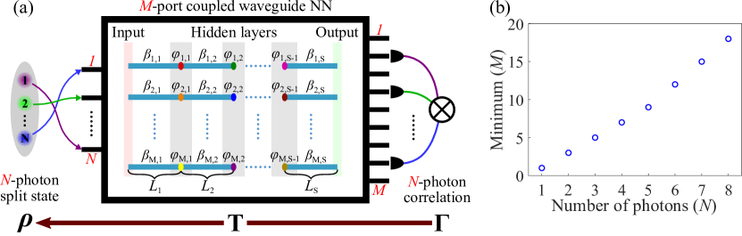
Figure 2: (a) Schematic of the proposed $M$-port coupled waveguide neural network for $N$-photon split state tomography, where the output $N$-photon correlations enable the reconstruction of the input density matrix. (b) Required number of waveguides for different photon numbers.

The proposed waveguide circuit is sketched inside the central frame in Fig. 2(a). It consists of $M$ waveguides, which optical modes are coupled to the nearest-neighbours with the constant coupling coefficient $\kappa$. The waveguides are segmented into $S$ sections with lengths $(L_{1},L_{2},\cdots,L_{S})$. We consider the presence of tailored phase shifts $\varphi_{i,j}$ at the interfaces between adjacent sections, noting that such localized shifts were demonstrated experimentally [38] and their incorporation was predicted to allow arbitrary unitary transformations [33, 39]. In addition, the design based on straight and identical waveguides ensures that there is no mismatch in the photon propagation lengths and dispersion, and the circuit is expected to better preserve the degree of photon indistinguishability during their interference compared to cascaded interferometers [40]. By design, the losses are expected to be similar for all waveguides, and we assume in the following that the output multi-photon correlations are above the noise level [35], which can be satisfied experimentally for at least $N=5$ photons [40]. Essentially, the configuration in Fig. 2(a) represents a linear artificial neural-network [41] with $S-1$ hidden layers, where each hidden layer has $M$ neurons. The waveguide couplings in each section function as the weights and the local phase shifts play similar roles to the bias.

The overall linear system transformation of the multi-photon state, provided that the losses are negligible, can be determined by a classical or one-photon unitary transfer matrix

$$\textbf{U}=\textbf{W}_{S}\leavevmode\nobreak\ \textbf{B}_{S-1}\leavevmode\nobreak\ \textbf{W}_{S-1}\leavevmode\nobreak\ \cdots\leavevmode\nobreak\ \textbf{B}_{2}\leavevmode\nobreak\ \textbf{W}_{2}\leavevmode\nobreak\ \textbf{B}_{1}\leavevmode\nobreak\ \textbf{W}_{1}\,.$$ (6)

Here $\textbf{W}_{j}=\exp(i\textbf{C}L_{j})$, calculated through the matrix exponent, is the weight matrix of the layer $j$, where the coupling matrix elements are $\textbf{C}_{n,m}=\kappa\delta_{n,m\pm 1}$. The bias matrix acting on the $j$-th hidden layer is $\textbf{B}_{j}=\exp(i\Phi_{j})$, where the exponent is applied element-wise to the phase shift matrix $\Phi_{j}={\rm diag}(\varphi_{1,j},\varphi_{2,j},\ldots,\varphi_{M,j})$. The $M\times M$ unitary matrix U can be flexibly tuned by varying the lengths of sections and local phase shifts.

For an $N$-photon split state, where the photons are coupled to specific $N$ ports at the input, its transformation is governed by N-in-M-out matrix $\textbf{U}_{r}$, which contains $N$ columns of U corresponding to the selected inputs. Then, we use a standard procedure [28, 29] to calculate the output $N$-photon correlations, which values can be represented by a vector $\vec{\Gamma}$ of the length equal to different combinations $M!/[N!(M-N)!]$. The correlations can be expressed through the independent elements of the input density matrix arranged in a vector $\vec{\rho}_{\rm free}$ of length $N!$,

$$\vec{\Gamma}=\textbf{T}\leavevmode\nobreak\ \vec{\rho}_{\rm free}\,,$$ (7)

where the matrix T is determined by $\textbf{U}_{r}$ and the structure of the split state density matrix.

Finally, we can reconstruct the input density matrix based on the measured $N$-photon correlations as

$$\vec{\rho}_{\rm free}=\textbf{T}^{+}\,\vec{\Gamma}\,,$$ (8)

where $\textbf{T}^{+}$ is the pseudoinverse of T.

It is essential to optimize the integrated circuit to reduce the reconstruction sensitivity to noise and measurement errors. Mathematically, this is achieved by minimizing the condition number of the matrix T, defined as the ratio of the transformation’s maximum and minimum singular values $\sigma_{max}(\textbf{T})/\sigma_{min}(\textbf{T})$ [42]. For our structure design, we perform numerical optimization of the waveguide section lengths and the local phase shifts based on the Nelder-Mead simplex direct search algorithm realized using the fminsearch function in Matlab.

IV Results and discussions

We performed extensive simulations of coupled-waveguide neural networks and found that tomography of split states with the photon number at least up to four can be efficiently performed in structures where all sections have the same length, all waveguides have the same propagation constants and thus zero detunings, and all the near-neighbour waveguide couplings are equal to each other. These conditions make the photonic circuit design and fabrication simpler, where all the waveguides have the same widths and the spacings between them are identical. We show in the following that optimization of the local phase shifts and the total waveguide length ($L$) allows us to reach low condition numbers, corresponding to low sensitivity to noise during the reconstruction. To simplify the notations, we consider the scaling of the waveguide length in the units of $\kappa^{-1}$, such that the coupling coefficient is normalized to one.

We first analyze the tomography of two-PSS. We choose the minimum required number of $M=3$ waveguides according to Eq. (5) and Fig. 2(b), select the first and third waveguides as the input ports, and consider a circuit structure with one hidden layer ($S=2$) as sketched in Fig. 3(a). We perform the optimization for different waveguide lengths and show the best condition number values in Fig. 3(b). One can see that the condition number reaches a minimum value of $\simeq 2.3$ when the waveguide length is longer than 0.84. This optimized condition number is smaller than the previously reported values for tomography of general two-photon states [26, 28]. The corresponding optimized phase shifts at the hidden layer are shown in Fig. 3(c), where we assign zero to one of the phases since the global phase does not affect the output correlations. Interestingly, all the three phase shifts are zero for the waveguide length shorter than 0.84, which effectively corresponds to the absence of hidden layer. For longer waveguides, the minimum value of condition number is achieved for circuits with an optimal hidden layer. For comparison, Fig. 3(d) shows the condition number for a structure without a hidden layer. We see that the circuit can allow for optimal performance over a broad range of structure lengths, offering more flexibility in integrating with other photonic components.

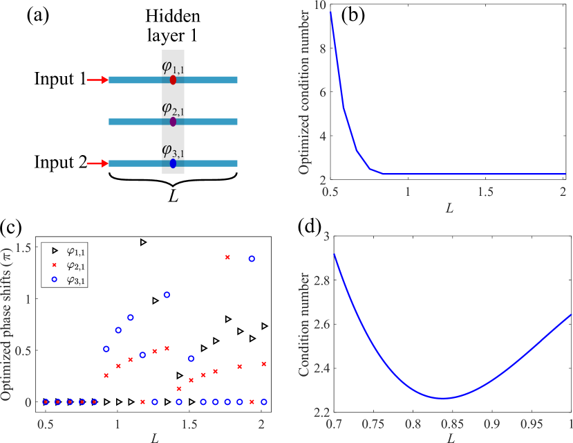
Figure 3: Optimized circuit for two-PSS tomography. (a) The structure of three coupled waveguides with one hidden layer. (b,c) Optimized (b) condition number and (c) phase shifts at the hidden layer as a function of the total waveguide length. (d) Condition number for a structure without a hidden layer vs. the waveguide length.

Next, we investigate the three-PSS tomography. Then, we use Eq. (5) to determine the required number of waveguides as $M=5$ and choose the first, third, and fifth waveguides as the input ports, see an illustration in Fig. 4(a). We check that without hidden layers, the condition number is very high, which would prevent a state reconstruction. The condition number dependencies on the structure length with the optimized one or two hidden layers are presented in Fig. 4(b). Overall, for a certain length, more hidden layers can provide lower condition numbers due to more tuning parameters. The smallest condition numbers are $\simeq 4.1$ at $L=2.5$ and $\simeq 3.9$ at $L=3$ for one and two hidden layers, respectively. These values are much smaller than the ones for general three-photon states [43]. The corresponding optimized phase shifts are $\varphi_{j,1}=(0,1.083,1.167,0.973,5.509)$ for one hidden layer and $\varphi_{j,1}=(0,4.248,3.808,1.442,5.098)$, $\varphi_{j,2}=(0,1.844,1.948,2.988,4.155)$ for two hidden layers.

We confirm the practicality of the designs by quantifying the tolerance of the optimal structures for three-PSS tomography to variations of the phase shifts due to potential fabrication errors. Figures 4(c) and 4(d) show the normalized probability density of the condition number values for random deviations of the phase shifts from the optimal values in different variation ranges. The white-colored numbers are the average condition numbers for different variation magnitudes. At small deviations, the structure with two hidden layers has better performance with the smaller condition number. In case of phase shift variations of $0.04\,\pi$ or larger, the structure with one hidden layer is better. This is because there are fewer phase shifts, and the performance is more robust to their variations. Overall, the condition numbers are smaller than 7, even when the phase shifts vary from the optimized values by a magnitude up to $0.1\pi$. This confirms the high fabrication tolerance of the circuits.

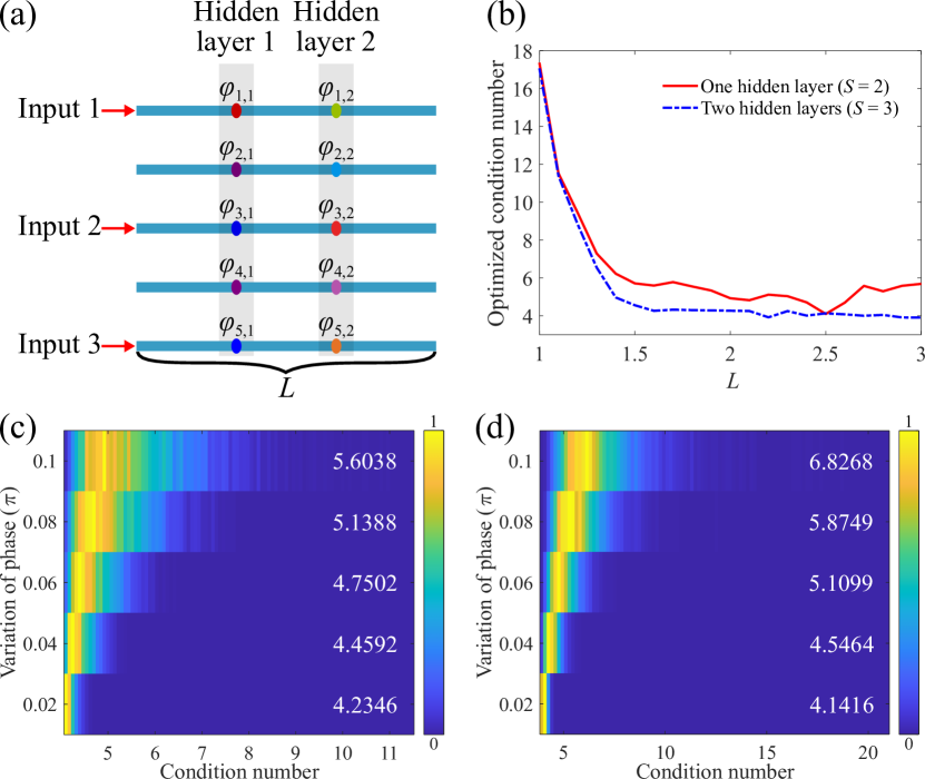
Figure 4: Tomography of three-PSS. (a) The structure of the 3-in-5-out couped-waveguide network with two hidden layers. (b) Optimized condition numbers vs. the total waveguide length with one or two hidden layers. (c,d) Normalized probability density of condition number values for 5000 simulations with random variations of the phase shifts from the optimal values for structures with (c) one hidden layer ($S=2$, $L=2.5$) and (d) two hidden layers ($S=3$, $L=3$). The vertical axis represents the magnitude of the random variations and the white-colored numbers are the corresponding averaged condition numbers.

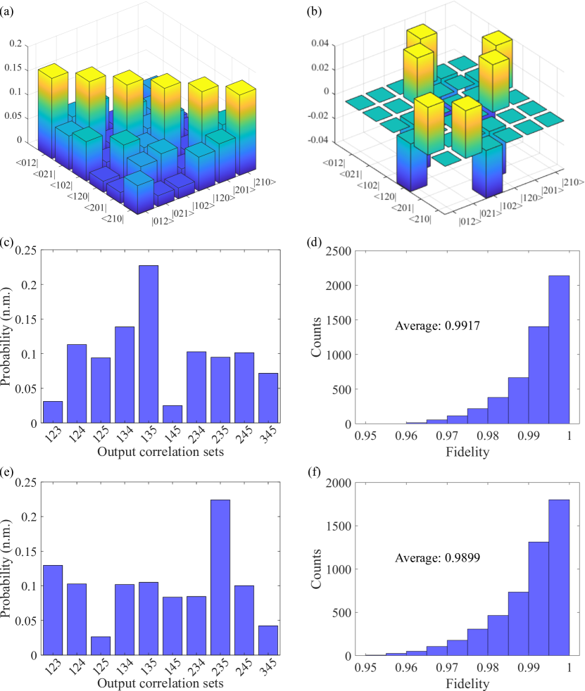
Figure 5: Three-photon reconstruction fidelity in presence of measurement noise. (a) Real and (b) imaginary parts of the density matrix for an input three-photon split state with a collective phase of $-\pi/3$. (c,e) The predicted three-photon correlation probabilities after passing through the optimized waveguide network. (d) The statistical distribution of the density matrix reconstruction fidelity for 5000 simulations when a Gaussian noise with a standard deviation of $5\%$ is added to the output correlations. Results correspond to the structures with (c,d) one and (e,f) two hidden layers.

Next, we demonstrate numerically the density matrix reconstruction of three-PSS. As an example, we consider the three-PSS composed of photons with uncorrelated frequency spectra, defined by the wavefunction $|\Psi\rangle=\int d\omega_{0}d\omega_{1}d\omega_{2}\phi_{0}(\omega_{0})\phi_{1}(\omega_{1})\phi_{2}(\omega_{2})\hat{a}_{0}^{\dagger}(\omega_{0})\hat{a}_{1}^{\dagger}(\omega_{1})\hat{a}_{2}^{\dagger}(\omega_{2})|0\rangle$, where $\phi_{j}(\omega)$ represents the spectral wavefunction of one photon in the $j$-th spatial path. In simulations, we assume the pairwise spectral overlaps as $\langle\phi_{0}|\phi_{1}\rangle=0.7e^{-i\pi/3}$, $\langle\phi_{1}|\phi_{2}\rangle=0.65$, and $\langle\phi_{2}|\phi_{0}\rangle=0.6$, which define all the spatial density matrix elements and the collective photon phase of $-\pi/3$ as formulated in Appendix B. The real and imaginary parts of the density matrix of this state are presented in Figs. 5(a) and 5(b), respectively. Figures 5(c) and 5(e) show the predicted three-photon correlation probabilities at the output of the optimized circuits with one and two hidden layers, respectively. We see that the correlations are different for each structure. Based on the output correlations, one can reconstruct the input density matrix. In order to verify the low sensitivity to the measurement noise, we apply a Gaussian noise to the correlations and use them to reconstruct the input density matrix. We quantify the quality of the tomography procedure by the fidelity between the reconstructed ($\rho_{rec}$) and the input ($\rho_{th}$) density matrices, defined as ${\rm Tr}(\sqrt{\sqrt{\rho_{th}}\rho_{rec}\sqrt{\rho_{th}}})$. Figures 5(d) and 5(f) show the corresponding statistical distributions of the reconstruction fidelity for 5000 simulations when a Gaussian noise with a standard deviation of $5\%$ is added to the predicted correlation probabilities. We find that the fidelity stays above 0.95 for both one- and two- hidden layer structures, with the average values of $\simeq 0.99$. We also confirm similarly high fidelity for different three-PSSs, including those with a zero collective phase. These results indicate the high accuracy of the tomographic reconstruction of split states under the presence of measurement noise.

The proposed approach and its high tolerance to fabrication errors and shot noise are also applicable to a larger number of photons. For example, we numerically designed a circuit with $N=4$, $M=7$, $S=3$, and $L=3$ for the tomography of four-PSS with an optimized condition number of 16.3464, for the hidden-layer phase shifts $\varphi_{j,1}=(0,1.126,0.306,4.331,4.990,1.633,2.419)$, $\varphi_{j,2}=(0,1.212,1.998,2.246,0.371,6.002,0.894)$

The designed circuits can be realized experimentally based on different integrated photonic platforms with established fabrication techniques. The localized phase shifts in coupled segmented waveguides were achieved through fs-laser writing in silica [38] and phase control using voids inside the waveguide was shown in silicon photonic circuits [44].

V Conclusion

To conclude, we have formulated the general structure of spatial density matrix for multi-photon split states, which are an important resource for various quantum applications and whose resource-efficient characterization is a sought-after capability. We then proposed a coupled waveguide array forming a photonic neural network for the quantum tomography of such states with low sensitivity to noise and high tolerance to fabrication errors. The state measurement can be performed using a static photonic circuit and this approach is scalable to high photon numbers.

We anticipate that the proposed platform, enabling simple and robust characterization of such commonly used quantum states, will stimulate further developments and applications of quantum optical circuits. In particular, since our scheme does not require reconfigurability, it is especially suitable for integration with on-chip superconducting nanowire single-photon detectors operating at cryogenic temperatures to facilitate plug-and-play split-state measurements. Furthermore, the theoretical methodology can be extended to the split states where photons are separated not only in spatial ports but also in other degrees of freedom, such as polarization and orbital angular momentum.

Appendix A Number of real and imaginary free parameters in density matrices of split states

As derived above, the number of nonzero elements in the reduced density matrix of $N$-photon split state equals to the distinct projection operators in the form of Eq. (3), and it is $N!$. The numbers of real and imaginary parts are determined by the numbers of nonzero distinct $(\hat{O}+\hat{O}_{H.C.})/2$ and $(\hat{O}-\hat{O}_{H.C.})/2$, respectively, where $H.C.$ stands for Hermitian conjugate [28]. To perform the counting, we define by $A_{N}$ the number of cases when $\hat{O}=\hat{O}_{H.C.}$, such that the related imaginary parts are zero. Next, we derive the recurrence relation for $A_{N}$ as a function of $N$. Let us consider the value of $s_{N-1}$. When $s_{N-1}=N-1$, the number of cases where $\hat{O}=\hat{O}_{H.C.}$ is $A_{N-1}$. When $s_{N-1}=\tilde{n}$ for $\tilde{n}=(0,1,\ldots,N-2)$, the condition $\hat{O}=\hat{O}_{H.C.}$ can only be satisfied when $s_{\tilde{n}}=N-1$. In this case, the number of cases where $\hat{O}=\hat{O}_{H.C.}$ becomes $A_{N-2}$. Since $\tilde{n}$ can take $N-1$ values, the total number is $(N-1)A_{N-2}$. Therefore, we obtain the relation

$$A_{N}=A_{N-1}+(N-1)A_{N-2}\quad{\rm for}\quad N\geq 3,$$ (9)

and the values for one- and two-photon states are $A_{1}=1$ and $A_{2}=2$.

Appendix B The spatial split-state density matrix for photons with uncorrelated frequency spectra

Whereas our approach is applicable to arbitrary multi-photon split states, here we discuss an example of states composed of photons with uncorrelated frequency spectra. Specifically, we consider a pure $N$-photon state

$$|\Psi\rangle=\int\,d\omega_{0}\,d\omega_{1}\,\cdots,d\omega_{N-1}\psi(\omega_{0},\omega_{1},\ldots\omega_{N-1})\hat{a}_{0}^{\dagger}(\omega_{0})\hat{a}_{1}^{\dagger}(\omega_{1})\cdots\hat{a}_{N-1}^{\dagger}(\omega_{N-1})|0\rangle\,$$ (10)

with the frequency-dependent wavefunction featuring no correlations between the individual spectra of photons,

$$\psi(\omega_{0},\omega_{1},\ldots,\omega_{N-1})=\phi_{0}(\omega_{0})\phi_{1}(\omega_{1})\cdots\phi_{N-1}(\omega_{N-1})\,.$$ (11)

Here $\phi_{j}(\omega_{j})$ is an individual spectral wavefunction of the photon coupled to a spatial mode number $j$.

We calculate the $N!$ nonzero elements of the first row of the reduced density matrix for the $N$-photon split state as

$$\begin{split}&{\rho_{0,1,\cdots,N-1;s_{0},s_{1},\cdots,s_{N-1}}={\rm Tr}\left(\hat{\rho}\,\hat{O}_{0,1,\cdots,N-1;s_{0},s_{1},\cdots,s_{N-1}}\right)}\\ &\quad{=\frac{1}{N!}\int d\omega_{0}d\omega_{1}\cdots d\omega_{N-1}\phi_{0}^{\ast}(\omega_{0})\phi_{1}^{\ast}(\omega_{1})\cdots\phi_{{N-1}}^{\ast}(\omega_{N-1})}{\phi_{{s_{0}}}(\omega_{0})\phi_{{s_{1}}}(\omega_{1})\cdots\phi_{{s_{N-1}}}(\omega_{N-1})}\\ &\quad{=\frac{1}{N!}I_{0,{s_{0}}}I_{1,{s_{1}}}\cdots I_{{N-1},{s_{N-1}}}}\,,\end{split}$$ (12)

where $(s_{0},s_{1},\cdots,s_{N-1})$ are permutations in the set $(0,1,\cdots,N-1)$ without repetition and we define the spectral overlaps between different photon pairs as

$$I_{i,j}=\langle\phi_{i}|\phi_{j}\rangle=\int d\omega\phi_{i}^{\ast}(\omega)\phi_{j}(\omega)\,,$$ (13)

with the normalization $I_{j,j}=1$.

For an $N=3$ photon case, we have

$${\rho_{0,1,2;0,1,2}=\frac{1}{6}}\,,\,\,{\rho_{0,1,2;0,2,1}=\frac{1}{6}|I_{1,2}|^{2}}\,,\,\,{\rho_{0,1,2;1,0,2}=\frac{1}{6}|I_{0,1}|^{2}}\,,\,\,{\rho_{0,1,2;2,1,0}=\frac{1}{6}|I_{2,0}|^{2}}\,,$$ (14)

$${\rho_{0,1,2;1,2,0}=\frac{1}{6}I_{0,1}I_{1,2}I_{2,0}}\,,\,\,{\rho_{0,1,2;2,0,1}=\frac{1}{6}I_{0,1}^{\ast}I_{1,2}^{\ast}I_{2,0}^{\ast}}.\quad$$

We see that the elements $\rho_{0,1,2;201}=\rho_{0,1,2;120}^{\ast}$ are related to the collective phase of three photons. Correspondingly, the six free parameters in Fig. 1(d) are

$${\rho_{1}=\rho_{0,1,2;0,1,2}},\quad{\rho_{2}=\rho_{0,1,2;0,2,1}},\quad{\rho_{3}=\rho_{0,1,2;1,0,2}}\,,$$ (15)

$${\rho_{4}={\rm Re}(\rho_{0,1,2;1,2,0})},\quad{\rho_{5}={\rm Im}(\rho_{0,1,2;1,2,0})},\quad{\rho_{6}=\rho_{0,1,2;2,1,0}}\,.$$

References

- Nielsen and Chuang [2011] M. A. Nielsen and I. L. Chuang, Quantum Computation and Quantum Information, 10th ed. (Cambridge University Press, Cambridge, 2011).
- Hong et al. [1987] C. K. Hong, Z. Y. Ou, and L. Mandel, Measurement of subpicosecond time intervals between 2 photons by interference, Phys. Rev. Lett. 59, 2044 (1987).
- Bouchard et al. [2021] F. Bouchard, A. Sit, Y. W. Zhang, R. Fickler, F. M. Miatto, Y. Yao, F. Sciarrino, and E. Karimi, Two-photon interference: the Hong-Ou-Mandel effect, Rep. Prog. Phys. 84, 012402 (2021).
- Menssen et al. [2017] A. J. Menssen, A. E. Jones, B. J. Metcalf, M. C. Tichy, S. Barz, W. S. Kolthammer, and I. A. Walmsley, Distinguishability and many-particle interference, Phys. Rev. Lett. 118, 153603 (2017).
- Spagnolo et al. [2013] N. Spagnolo, C. Vitelli, L. Aparo, P. Mataloni, F. Sciarrino, A. Crespi, R. Ramponi, and R. Osellame, Three-photon bosonic coalescence in an integrated tritter, Nat. Commun. 4, 1606 (2013).
- Brod et al. [2019] D. J. Brod, E. F. Galvao, N. Viggianiello, F. Flamini, N. Spagnolo, and F. Sciarrino, Witnessing genuine multiphoton indistinguishability, Phys. Rev. Lett. 122, 063602 (2019).
- Pont et al. [2022] M. Pont, R. Albiero, S. E. Thomas, N. Spagnolo, F. Ceccarelli, G. Corrielli, A. Brieussel, N. Somaschi, H. Huet, A. Harouri, A. Lemaitre, I. Sagnes, N. Belabas, F. Sciarrino, R. Osellame, P. Senellart, and A. Crespi, Quantifying n-photon indistinguishability with a cyclic integrated interferometer, Phys. Rev. X 12, 031033 (2022).
- Giordani et al. [2020] T. Giordani, D. J. Brod, C. Esposito, N. Viggianiello, M. Romano, F. Flamini, G. Carvacho, N. Spagnolo, E. F. Galvao, and F. Sciarrino, Experimental quantification of four-photon indistinguishability, New J. Phys. 22, 043001 (2020).
- Spring et al. [2013] J. B. Spring, B. J. Metcalf, P. C. Humphreys, W. S. Kolthammer, X. M. Jin, M. Barbieri, A. Datta, N. Thomas-Peter, N. K. Langford, D. Kundys, J. C. Gates, B. J. Smith, P. G. R. Smith, and I. A. Walmsley, Boson sampling on a photonic chip, Science 339, 798 (2013).
- Broome et al. [2013] M. A. Broome, A. Fedrizzi, S. Rahimi-Keshari, J. Dove, S. Aaronson, T. C. Ralph, and A. G. White, Photonic boson sampling in a tunable circuit, Science 339, 794 (2013).
- Tillmann et al. [2013] M. Tillmann, B. Dakic, R. Heilmann, S. Nolte, A. Szameit, and P. Walther, Experimental boson sampling, Nat. Photon. 7, 540 (2013).
- Crespi et al. [2013] A. Crespi, R. Osellame, R. Ramponi, D. J. Brod, E. F. Galvao, N. Spagnolo, C. Vitelli, E. Maiorino, P. Mataloni, and F. Sciarrino, Integrated multimode interferometers with arbitrary designs for photonic boson sampling, Nat. Photon. 7, 545 (2013).
- Shchesnovich [2015a] V. S. Shchesnovich, Tight bound on the trace distance between a realistic device with partially indistinguishable bosons and the ideal bosonsampling, Phys. Rev. A 91, 063842 (2015a).
- Renema et al. [2018] J. J. Renema, A. Menssen, W. R. Clements, G. Triginer, W. S. Kolthammer, and I. A. Walmsley, Efficient classical algorithm for boson sampling with partially distinguishable photons, Phys. Rev. Lett. 120, 220502 (2018).
- Shchesnovich and Bezerra [2018] V. S. Shchesnovich and M. E. O. Bezerra, Collective phases of identical particles interfering on linear multiports, Phys. Rev. A 98, 033805 (2018).
- Jones et al. [2020] A. E. Jones, A. J. Menssen, H. M. Chrzanowski, T. A. W. Wolterink, V. S. Shchesnovich, and I. A. Walmsley, Multiparticle interference of pairwise distinguishable photons, Phys. Rev. Lett. 125, 123603 (2020).
- Altepeter et al. [2005] J. B. Altepeter, E. R. Jeffrey, and P. G. Kwiat, Photonic state tomography, Adv. Atom. Mol. Opt. Phys. 52, 105 (2005).
- Lvovsky and Raymer [2009] A. I. Lvovsky and M. G. Raymer, Continuous-variable optical quantum-state tomography, Rev. Mod. Phys. 81, 299 (2009).
- Toninelli et al. [2019] E. Toninelli, B. Ndagano, A. Valles, B. Sephton, I. Nape, A. Ambrosio, F. Capasso, M. J. Padgett, and A. Forbes, Concepts in quantum state tomography and classical implementation with intense light: a tutorial, Adv. Opt. Photon. 11, 67 (2019).
- Teo et al. [2021] Y. S. Teo, S. Shin, H. Jeong, Y. Kim, Y. H. Kim, G. I. Struchalin, E. V. Kovlakov, S. S. Straupe, S. P. Kulik, G. Leuchs, and L. L. Sanchez-Soto, Benchmarking quantum tomography completeness and fidelity with machine learning, New J. Phys. 23, 103021 (2021).
- James et al. [2001] D. F. V. James, P. G. Kwiat, W. J. Munro, and A. G. White, Measurement of qubits, Phys. Rev. A 64, 052312 (2001).
- Shadbolt et al. [2012] P. J. Shadbolt, M. R. Verde, A. Peruzzo, A. Politi, A. Laing, M. Lobino, J. C. F. Matthews, M. G. Thompson, and J. L. O’Brien, Generating, manipulating and measuring entanglement and mixture with a reconfigurable photonic circuit, Nat. Photon. 6, 45 (2012).
- D’Ariano [2002] G. M. D’Ariano, Universal quantum observables, Phys. Lett. A 300, 1 (2002).
- Allahverdyan et al. [2004] A. E. Allahverdyan, R. Balian, and T. M. Nieuwenhuizen, Determining a quantum state by means of a single apparatus, Phys. Rev. Lett. 92, 120402 (2004).
- D’Ariano et al. [2004] G. M. D’Ariano, P. Perinotti, and M. F. Sacchi, Quantum universal detectors, Europhys. Lett. 65, 165 (2004).
- Titchener et al. [2016] J. G. Titchener, A. S. Solntsev, and A. A. Sukhorukov, Two-photon tomography using on-chip quantum walks, Opt. Lett. 41, 4079 (2016).
- Banchi et al. [2018] L. Banchi, W. S. Kolthammer, and M. S. Kim, Multiphoton tomography with linear optics and photon counting, Phys. Rev. Lett. 121, 250402 (2018).
- Titchener et al. [2018] J. G. Titchener, M. Grafe, R. Heilmann, A. S. Solntsev, A. Szameit, and A. A. Sukhorukov, Scalable on-chip quantum state tomography, npj Quant. Inform. 4, 19 (2018).
- Wang et al. [2018] K. Wang, J. G. Titchener, S. S. Kruk, L. Xu, H. P. Chung, M. Parry, I. I. Kravchenko, Y. H. Chen, A. S. Solntsev, Y. S. Kivshar, D. N. Neshev, and A. A. Sukhorukov, Quantum metasurface for multiphoton interference and state reconstruction, Science 361, 1104 (2018).
- Shchesnovich [2014] V. S. Shchesnovich, Sufficient condition for the mode mismatch of single photons for scalability of the boson-sampling computer, Phys. Rev. A 89, 022333 (2014).
- Shchesnovich [2015b] V. S. Shchesnovich, Partial indistinguishability theory for multiphoton experiments in multiport devices, Phys. Rev. A 91, 013844 (2015b).
- Christodoulides et al. [2003] D. N. Christodoulides, F. Lederer, and Y. Silberberg, Discretizing light behaviour in linear and nonlinear waveguide lattices, Nature 424, 817 (2003).
- Zhou et al. [2018] J. H. Zhou, J. J. Wu, and Q. S. Hu, Tunable arbitrary unitary transformer based on multiple sections of multicore fibers with phase control, Opt. Express 26, 3020 (2018).
- Skryabin et al. [2021] N. N. Skryabin, I. V. Dyakonov, M. Y. Saygin, and S. P. Kulik, Waveguide-lattice-based architecture for multichannel optical transformations, Opt. Express 29, 26058 (2021).
- Garcia-Patron et al. [2019] R. Garcia-Patron, J. J. Renema, and V. Shchesnovich, Simulating boson sampling in lossy architectures, Quantum 3, 169 (2019).
- Clements et al. [2016] W. R. Clements, P. C. Humphreys, B. J. Metcalf, W. S. Kolthammer, and I. A. Walsmley, Optimal design for universal multiport interferometers, Optica 3, 1460 (2016).
- Lahini et al. [2018] Y. Lahini, G. R. Steinbrecher, A. D. Bookatz, and D. Englund, Quantum logic using correlated one-dimensional quantum walks, npj Quant. Inform. 4, 2 (2018).
- Szameit et al. [2008] A. Szameit, F. Dreisow, M. Heinrich, T. Pertsch, S. Nolte, A. Tunnermann, E. Suran, F. Louradour, A. Barthelemy, and S. Longhi, Image reconstruction in segmented femtosecond laser-written waveguide arrays, Appl. Phys. Lett. 93, 181109 (2008).
- Saygin et al. [2020] M. Y. Saygin, I. V. Kondratyev, I. V. Dyakonov, S. A. Mironov, S. S. Straupe, and S. P. Kulik, Robust architecture for programmable universal unitaries, Phys. Rev. Lett. 124, 010501 (2020).
- Bell et al. [2019] B. A. Bell, G. S. Thekkadath, R. Y. Ge, X. L. Cai, and I. A. Walmsley, Testing multi-photon interference on a silicon chip, Opt. Express 27, 35646 (2019).
- Steinbrecher et al. [2019] G. R. Steinbrecher, J. P. Olson, D. Englund, and J. Carolan, Quantum optical neural networks, npj Quant. Inform. 5, 60 (2019).
- Press et al. [2007] W. H. Press, S. A. Teukolsky, W. T. Vetterling, and B. P. Flannery, Numerical Recipes: The Art of Scientific Computing, 3rd ed. (Cambridge University Press, Cambridge, 2007).
- Wang et al. [2019a] K. Wang, S. V. Suchkov, J. G. Titchener, A. Szameit, and A. A. Sukhorukov, Inline detection and reconstruction of multiphoton quantum states, Optica 6, 41 (2019a).
- Wang et al. [2019b] Z. Wang, T. T. Li, A. Soman, D. Mao, T. Kananen, and T. Y. Gu, On-chip wavefront shaping with dielectric metasurface, Nat. Commun. 10, 3547 (2019b).