Excitations of the ferroelectric order

Abstract

We identify the bosonic excitations in ferroelectrics that carry electric dipoles from the phenomenological Landau-Ginzburg-Devonshire theory. The “ferron” quasi-particles emerge from the concerted action of anharmonicity and broken inversion symmetry. In contrast to magnons, the transverse excitations of the magnetic order, the ferrons in displacive ferroelectrics are longitudinal with respect to the ferroelectric order. Based on the ferron spectrum, we predict temperature dependent pyroelectric and electrocaloric properties, electric-field-tunable heat and polarization transport, and ferron-photon hybridization.

The spontaneous emergence of order in condensed matter below a critical temperature breaks a symmetry, while the low-energy collective excitations of the order parameter tend to restore it. The latter can often be modeled by non-interacting quasi-particles that in extended system are plane waves with a well-defined dispersion relation. Their lifetime is finite due to self-interactions or coupling with the environment. Wave packets of these quasiparticles transport energy, momentum, and order parameter with the group velocity from the dispersion relations.

Lattice vibrations disturb the translational symmetry of homogeneous elastic media, and phonons are the associated quasi-particles. The excitations of a magnetic order are spin waves. The associated quanta, the magnons, carry magnetic moments that reduce the magnetization and can transport spin angular momentum and energy Kruglyak et al. (2010); Chumak et al. (2015). Gradients of temperature and magnon chemical potential Cornelissen et al. (2015, 2016) induce magnon spin and heat currents, with associated spin Seebeck Uchida et al. (2010) and spin Peltier Flipse et al. (2014); Daimon et al. (2016) effects.

Ferroelectric materials exhibit ordered electric dipoles with unique dielectric, pyroelectric, piezoelectric and electrocaloric properties Xu (2013), with many analogies with ferromagnets Spaldin (2007). However, to the best of our knowledge, the quasi-particles associated to the ferroelectric order have so far remained elusive. We previously addressed the elementary excitations of ferroelectrics or “ferrons” and the associated polarization and heat transport Bauer et al. (2021); Tang et al. (2021) by a phenomenological diffusion equation and a simple ball-spring model. The latter was inspired by magnons, which are transverse fluctuations that preserve the magnitude of the local magnetization. The assumption of local electric dipoles with fixed modulus should hold for order-disorder ferroelectrics such as NaNO₂ that are formed by stable molecular dipoles Blinc and Žekš (1972). However, most ferroelectrics are “displacive”, i.e., formed by the condensation of a particular soft phonon Cochran (1959, 1960) with a flexible dipole moment (or are of mixed type Müller et al. (1982); Dalal et al. (1998); Zalar et al. (2003); Bussmann-Holder et al. (2009)), and cannot be described by our previous model.

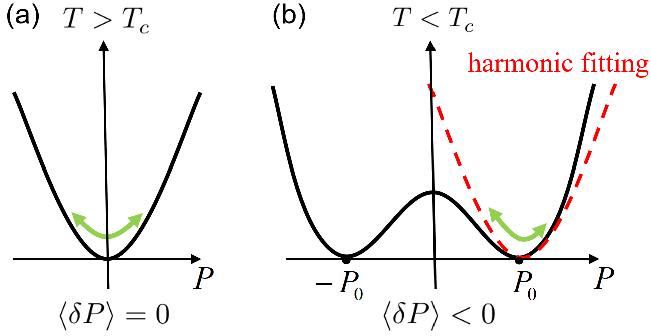
Figure 1: Landau potential energy landscape for polarization fluctuations in ferroelectrics (green arrows). (a) Above the critical temperature $T_{c}$ in the paraelectric phase the potential is symmetric for the fluctuations around the minimum $P_{0}=0$ and the average of the fluctuations $\langle\delta P\rangle=\langle P-P_{0}\rangle=0$ even in the presence of anharmonicity (see Eq. (8)). (b) Below $T_{c}$ the ferroelectric order breaks inversion symmetry and polarization fluctuates around finite $\pm P_{0}$ (e.g., the positive one in the figure) in an asymmetric potential, therefore carrying a non-vanishing average electric dipoles, i.e., $\langle\delta P\rangle=\langle P-P_{0}\rangle<0$.

In this Letter, we formulate the quasi-particle excitations of displacive ferroelectrics in the framework of the Landau-Ginzburg-Devonshire (LGD) theory Devonshire (1949, 1951), which has been widely used to model ferroelectrics over a broad temperature range Salje (1990). These ferrons are longitudinal rather than transverse fluctuations and carry electric polarization because of the non-parabolicity of the free energy around the local minima below the phase transition (see Fig. 1). The parameters of the LGD free energy are well-known for many materials, which allows quantitative predictions of their thermodynamic and transport properties.

Model: The LGD free energy $F(\mathbf{P})$ for a ferroelectric is a functional of the macroscopic polarization texture $\mathbf{P}(\mathbf{r})$ that obeys the crystal symmetry of the parent paraelectric phase Cao (2008). For a uniaxial ferroelectric formed out of a centrosymmetric paraelectric phase the (Gibbs) free energy is an integral over the sample volume $V$ Chandra and Littlewood (2007):

$$F=\int d^{3}\mathbf{r}\left(\frac{g}{2}(\nabla\mathbf{P})^{2}+\frac{\alpha}{2}P^{2}+\frac{\beta}{4}P^{4}+\frac{\lambda}{6}P^{6}-\mathbf{E}\cdot\mathbf{P}\right),$$ (1)

where $\alpha$, $\beta$ and $\lambda>0$ are the Landau coefficients, $g>0$ is the Ginzburg-type parameter that accounts for the energy cost of polarization textures and $\mathbf{E}$ an external electric field. A constant spontaneous polarization $(\mathbf{P}_{0})$ minimizes $F(\mathbf{P})$ of a uniform medium when

$$\alpha P_{0}+\beta P_{0}^{3}+\lambda P_{0}^{5}=E$$ (2)

where $P_{0}$ ($E$) is the modulus of the vectors $\mathbf{P}_{0}$ ($\mathbf{E}$) and $\mathbf{E\|P}_{0}.$ Below a critical temperature $T_{c}$ the system orders in a first (second)-order phase transition for $\beta<0$ ($\beta>0$) with $P_{0}^{2}=\left(-\beta+\sqrt{\beta^{2}-4\alpha\lambda}\right)/2\lambda$ for $E=0$.

In the presence of fluctuations, the longitudinal polarization dynamics ($\mathbf{P}\|\mathbf{P}_{0}$) obeys the Landau-Khalatnikov-Tani equation Tani (1969); Ishibashi (1989); Sivasubramanian et al. (2004); Widom et al. (2010),

$$m_{p}\frac{\partial^{2}P}{\partial t^{2}}+\gamma\frac{\partial P}{\partial t}=-\frac{\partial F}{\partial P}+E_{\mathrm{th}},$$ (3)

where $m_{p}=(\varepsilon_{0}\omega_{p}^{2})^{-1}$ is the polarization inertia, $\varepsilon_{0}$ the vacuum dielectric constant, and $\gamma$ a phenomenological damping constant. The plasma frequency $\omega_{p}$ depends on the ionic masses $M_{i}$ and charges $Q_{i}$ in the unit cell of volume $V_{0}$ as $\omega_{p}^{2}=(\varepsilon_{0}V_{0})^{-1}\sum_{i}Q_{i}^{2}/M_{i}$ Sivasubramanian et al. (2004). $E_{\mathrm{th}}(\mathbf{r},t)$ is a Langevin noise field that obeys a fluctuation-dissipation theorem Landau et al. (1980),

$$\langle E_{\mathrm{th}}(\mathbf{q},\omega) E_{\mathrm{th}}^{\ast}(\mathbf{q}^{\prime},\omega^{\prime})\rangle=\frac{(2\pi)^{4}\gamma\hbar\omega\delta(\mathbf{q}-\mathbf{q}^{\prime})\delta(\omega-\omega^{\prime})}{\tanh(\hbar\omega/2k_{B}T)}$$

$$\overset{k_{B}T\gg\hbar\omega}{\rightarrow}(2\pi)^{4}2\gamma k_{B}T\delta(\mathbf{q}-\mathbf{q}^{\prime})\delta(\omega-\omega^{\prime}),$$ (4)

where $\langle\cdots\rangle$ is an ensemble average, $E_{\mathrm{th}}(\mathbf{q},\omega)=\int dt\int d^{3}\mathbf{r}E_{\mathrm{th}}(\mathbf{r},t)e^{-i\mathbf{q}\cdot\mathbf{r}+i\omega t}$ the Fourier component of $E_{\mathrm{th}}(\mathbf{r},t)$ and the second line indicates the classical white noise limit. Substituting the small fluctuations $\delta P(\mathbf{r},t)=P(\mathbf{r},t)-P_{0}$ into Eq. (3):

$$\hat{G}^{-1}\delta P=E_{\mathrm{th}}-\left(3\beta+10\lambda P_{0}^{2}\right)P_{0}\delta P^{2}+\mathcal{O}(\delta P^{3})$$ (5)

where $\hat{G}^{-1}\equiv m_{p}\partial_{t}^{2}+\gamma\partial_{t}-g\nabla^{2}+(\alpha+3\beta P_{0}^{2}+5\lambda P_{0}^{4})$ is an inverse propagator. The non-linear terms on the right-hand side of Eq. (5) are proportional to the anharmonicity parameters $\beta$ and $\lambda$ in Eq. (1). At temperatures sufficiently below the $T_{c}$ the fluctuations $E_{\mathrm{th}}$ are small and we may solve Eq. (5) iteratively. To leading order,

$$\delta P=\delta P_{\mathrm{h}}-\left(3\beta+10\lambda P_{0}^{2}\right)P_{0}\hat{G}\delta P_{\mathrm{h}}^{2}+\mathcal{O}(E_{\mathrm{th}}^{3})$$ (6)

where $\delta P_{\mathrm{h}}\equiv\hat{G}E_{\mathrm{th}}$ are the harmonic thermal fluctuations that on average do not change the polarization since $\left\langle\delta P_{\mathrm{h}}\right\rangle=0$. In Fourier space

$$\delta P_{\mathrm{h}}(\mathbf{q},\omega)=\frac{E_{\mathrm{th}}(\mathbf{q},\omega)}{m_{p}(\omega_{\mathbf{q}}^{2}-\omega^{2})-i\omega\gamma}$$ (7)

where $\omega_{\mathbf{q}}=m_{p}^{-1/2}(\alpha+3\beta P_{0}^{2}+5\lambda P_{0}^{4}+g\mathbf{q}^{2})^{1/2}$ is the dispersion relation. Assuming weak dissipation $\gamma\ll m_{p}\omega_{\mathbf{q}}$, Eqs. (Excitations of the ferroelectric order), (6) and (7) leads to fluctuations

$$\langle\delta P\rangle=-\frac{\hbar(3\beta+10\lambda P_{0}^{2})P_{0}}{2m_{p}(\alpha+3\beta P_{0}^{2}+5\lambda P_{0}^{4})}\int\frac{d^{3}\mathbf{q}}{(2\pi)^{3}}\frac{1}{\omega_{\mathbf{q}}}\coth\frac{\hbar\omega_{\mathbf{q}}}{2k_{B}T}$$ (8)

that suppress the ground state polarization $P_{0}$ because of the anharmonicity, see Fig. 1. We may quantize the harmonic fluctuations as

$$\delta\hat{P}_{\mathrm{h}}=\sqrt{\frac{\hbar}{2m_{p}V}}\sum_{\mathbf{q}}\hat{a}_{\mathbf{q}}\frac{e^{i\mathbf{q}\cdot\mathbf{r}}}{\sqrt{\omega_{\mathbf{q}}}}+\mathrm{H.c}{\normalsize.}$$ (9)

where $\hat{a}_{\mathbf{q}}$ ($\hat{a}_{\mathbf{q}}^{\dagger}$) represents the bosonic annihilation (creation) operator of “ferrons” with wave vector $\mathbf{q}$ and frequency $\omega_{\mathbf{q}}$. After substracting the zero-point fluctuations, the elementary electric dipole carried by a single ferron is $\delta p_{\mathbf{q}}=\langle\mathbf{q}|\delta\hat{P}|\mathbf{q}\rangle-\langle 0|\delta\hat{P}|0\rangle$, where $|\mathbf{q}\rangle=\hat{a}_{\mathbf{q}}^{\dagger}|0\rangle$ and $|0\rangle$ the vacuum. By substituting Eq. (9) into Eq. (6),

$$\delta p_{\mathbf{q}}=-\frac{\hbar(3\beta+10\lambda P_{0}^{2})P_{0}}{m_{p}(\alpha+3\beta P_{0}^{2}+5\lambda P_{0}^{4})}\frac{1}{\omega_{\mathbf{q}}}.$$ (10)

Using the non-linear dielectric susceptibility $\chi=\partial P_{0}/\partial E=(\alpha+3\beta P_{0}^{2}+5\lambda P_{0}^{4})^{-1}$ that follows from Eq. (2), Eq. (10) can be rewritten as

$$\delta p_{\mathbf{q}}=\frac{\hbar}{2m_{p}}\frac{\partial\ln\chi}{\partial P_{0}}\frac{1}{\omega_{\mathbf{q}}}.$$ (11)

Eq. (10) and Eq. (11) agree with the intuitive relation

$$\delta p_{\mathbf{q}}=-\frac{\partial\hbar\omega_{\mathbf{q}}}{\partial E}$$ (12)

which also holds for $E\neq 0$. According to Eq. (10) the ferron electric dipole reduces $\mathbf{P}_{0}$ (i.e., $\partial\ln\chi/\partial P_{0}<0$) and emerges from the anharmonicity of the free energy below the phase transition. As in order-disorder ferroelectrics Bauer et al. (2021); Tang et al. (2021) and in contrast to the magnetic dipole associated to magnons, the electric dipole of the longitudinal ferrons depends strongly and non-universally on the wave vector. In the paraelectric phase, the spontaneous polarization vanishes and hence $\delta p_{\mathbf{q}}=0$, but a strong enough applied external field polarizes the paraelectric state and its elementary excitations as well.

The expansion to leading order in the amplitudes limits quantitative predictions to temperatures sufficiently below $T_{c}$. However, we may profit in the future from the large knowledge base on computing phononic non-linearities in complex materials Tadano and Tsuneyuki (2018).

We assume dominance of a single-band soft mode that triggers the symmetry-breaking structural phase transitions to the ferroelectric state. In displacive ferroelectrics this is the lowest soft optical phonon that vibrates parallel to $\mathbf{P}_{0}$. Hybridization with other, such as acoustic, phonon modes can become significant for some physical properties Tang and Bauer .

The free energy Eq. (1) does not introduce non-parabolicities to the transverse oscillations, which therefore do not carry any dipolar moment. Order-disorder ferroelectrics can also be treated by Landau theory, but polarized fluctuations only emerge by introducing non-linearities in the transverse amplitudes. At sufficiently low temperatures this can conveniently be achieved by the constraint $\left|\mathbf{P}\right|=P_{0}$, which to leading order gives rise to a finite dipole of the transverse ferrons, analogous to the magnetic moment of magnons Bauer et al. (2021); Tang et al. (2021). Longitudinal and transverse ferrons may coexist in some multiaxial materials.

Since the LGD parameters are well documented for many ferroelectric materials Haun et al. (1987); Pertsev et al. (1998); Scrymgeour et al. (2005); Li et al. (2005); Hlinka and Marton (2006); Liang et al. (2009), we are in an excellent position to quantitatively study ferron-related thermodynamic, optical, and transport properties. Table 1 summarizes the key information for selected displacive ferroelectrics with perovskite crystal structure at room temperature.

Pyroelectricity and electrocalorics. Pyroelectricity (electrocalorics) is the change of polarization (entropy) under a temperature (electric field) change Whatmore (1986); Muralt (2001); Mischenko et al. (2006); Neese et al. (2008); Li et al. (2020). They are conventionally calculated directly by the LGD free energy with linear temperature dependence of the Landau quadratic coefficient ($\alpha$) Muralt (2001); Li et al. (2020). However, this approach is valid only near the phase transition. At lower temperatures the fluctuations are well represented by the ferrons, and $\alpha$ becomes temperature independent. The total polarization is $P(T)=P(0)+\Delta P(T)$ with

$$\Delta P(T) =\int\frac{d^{3}\mathbf{q}}{(2\pi)^{3}}f_{0}\left(\xi_{\mathbf{q}}\right)\delta p_{\mathbf{q}}$$

$$\rightarrow-\frac{\hbar(3\beta+10\lambda P_{0}^{2})P_{0}}{(2\pi g)^{3/2}m_{p}^{1/2}}\frac{1}{\xi_{0}^{3/2}}\exp\left(-\xi_{0}\right),$$ (13)

where $f_{0}(\xi_{\mathbf{q}})=[\exp(\xi_{\mathbf{q}})-1]^{-1}$ is the Planck distribution, $\xi_{\mathbf{q}}=\hbar\omega_{\mathbf{q}}/k_{B}T$ and in the second step we took the low temperature limit $\xi_{0}=\hbar\omega_{0}/k_{B}T\gg 1$ with $\omega_{0}=m_{p}^{-1/2}(\alpha+3\beta P_{0}^{2}+5\lambda P_{0}^{4})^{1/2}$ the ferron gap (at $E=0$). By disregarding the temperature dependence of material parameters, the low-temperature pyroelectric coefficient we arrive at the thermally activated form

$$\frac{\partial\Delta P}{\partial T}\rightarrow-\frac{(\hbar k_{B})^{1/2}(3\beta+10\lambda P_{0}^{2})P_{0}}{(2\pi g)^{3/2}(m_{p}\omega_{0})^{1/2}}\frac{1}{\sqrt{T}}\exp\left(-\xi_{0}\right).$$ (14)

The electrocaloric coefficient, i.e. the isothermal entropy change with electric field, is according to the Maxwell relation

$$\left(\frac{\partial\Delta S}{\partial E}\right)_{T}=\left(\frac{\partial\Delta P}{\partial T}\right)_{E}.$$ (15)

The temperature dependence deviates strongly from a Curie-Weiss power-law. Glass and Lines Glass and Lines (1976) derived the scaling relation Eq. (14) in order to explain the low-temperature pyroelectricity of LiNbO₃ and LiTaO${}_{3},$ thereby implicitly introducing the ferron concept for equilibrium properties a long time ago. Lang et al. Lang et al. (1969) observed a negative pyroelectric coefficient in BaTiO₃ ceramic at low temperature, whose absolute value increases exponentially with temperature, in qualitative agreement with Eq. (14). However, the experimental $\partial\Delta P/\partial T=-5\times 10^{-7}$ C/(m²K) at $4.9$ K is much larger than Eq. (14), which has been ascribed to a polarization of acoustic phonons coupled to the soft mode Born (1945); Szigeti (1975). 

Polarization and heat transport by ferrons. We consider here diffuse and ballistic ferron transport in bulk ferroelectrics Bauer et al. (2021) and through constrictions Tang et al. (2021), respectively. In the former case we focus on homogeneous single-domain ferroelectrics at local thermal equilibrium with an electric field generated by internal polarization and external charges. Electric field ($\partial E$) and temperature ($\partial T$) gradients set along the $x$ direction induce polarization $\left(j_{p}\right)$ and heat $\left(j_{q}\right)$ current densities. The driving forces include non-equilibrium contributions from polarization and heat accumulations that should be computed self-consistently Bauer et al. (2021). We can derive the polarization $\left(\sigma\right)$ and thermal $\left(\kappa\right)$ conductivities and the Seebeck $\left(S_{d}\right)$ and Peltier $\left(\Pi_{d}\right)$ coefficients in the linear response relations

$$\left(\begin{matrix}-j_{p}\\ j_{q}\end{matrix}\right)=\sigma\left(\begin{matrix}1&S_{d}\\ \Pi_{d}&\kappa/\sigma\end{matrix}\right)\left(\begin{matrix}\partial E\\ -\partial T\end{matrix}\right)$$ (16)

by the Landau theory introduced above. The linearized Boltzmann transport equation of the ferron gas in a constant relaxation time approximation Bauer et al. (2022) yields

$$\sigma =\frac{\tau}{\hbar}\int(v_{\mathbf{q}}^{x})^{2}(\delta p_{\mathbf{q}})^{2}\left(-\frac{\partial f_{0}}{\partial\omega_{\mathbf{q}}}\right)\frac{d^{3}\mathbf{q}}{(2\pi)^{3}}$$

$$=\frac{\tau\hbar}{8\pi^{2}m_{p}^{3/2}g^{1/2}}\left[\frac{\partial\ln\chi}{\partial P_{0}}\right]^{2}\left\{\begin{array}[c]{c}\sqrt{\frac{\pi}{2}}\xi_{0}^{-3/2}e^{-\xi_{0}},\\ \frac{\pi}{16}\xi_{0}^{-1},\end{array}\begin{array}[c]{c}\xi_{0}\gg 1\\ \xi_{0}\ll 1\end{array}\right.$$ (21)

$$S_{d} =\frac{\tau}{\hbar(\sigma T)}\int(v_{\mathbf{q}}^{x})^{2}(-\delta p_{\mathbf{q}})\hbar\omega_{\mathbf{q}}\left(-\frac{\partial f_{0}}{\partial\omega_{\mathbf{q}}}\right)\frac{d^{3}\mathbf{q}}{(2\pi)^{3}}$$

$$=\frac{\tau k_{B}^{2}T}{12\pi^{2}\hbar(m_{p}g)^{1/2}\sigma}\frac{\partial\ln\chi}{\partial P_{0}}\left\{\begin{array}[c]{c}3\sqrt{\frac{\pi}{2}}\xi_{0}^{1/2}e^{-\xi_{0}},\\ \frac{\pi^{2}}{3},\end{array}\begin{array}[c]{c}\xi_{0}\gg 1\\ \xi_{0}\ll 1\end{array}\right.$$ (26)

$$\kappa =\frac{\tau}{\hbar T}\int(v_{\mathbf{q}}^{x})^{2}(\hbar\omega_{\mathbf{q}})^{2}\left(-\frac{\partial f_{0}}{\partial\omega_{\mathbf{q}}}\right)\frac{d^{3}\mathbf{q}}{(2\pi)^{3}}$$

$$=\frac{\tau k_{B}^{4}T^{3}m_{p}^{1/2}}{6\pi^{2}\hbar^{3}g^{1/2}}\left\{\begin{array}[c]{c}3\sqrt{\frac{\pi}{2}}\xi_{0}^{5/2}e^{-\xi_{0}},\\ \frac{4\pi^{4}}{15},\end{array}\begin{array}[c]{c}\xi_{0}\gg 1\\ \xi_{0}\ll 1\end{array}\right.$$ (31)

and the Kelvin-Onsager relation $\Pi_{d}=TS_{d}$. Here $\tau$ is the ferron relaxation time, $v_{\mathbf{q}}^{x}=\partial\omega_{\mathbf{q}}/\partial q_{x}=gq_{x}/(m_{p}\omega_{\mathbf{q}})$ the group velocity in the tranport $(x)$ direction. We may define a Lorenz number

$$L_{d}\equiv\frac{\kappa}{\sigma T}=\frac{4m_{p}^{2}k_{B}^{4}T^{2}}{\hbar^{4}}\left[\frac{\partial\ln\chi}{\partial P_{0}}\right]^{-2}\left\{\begin{array}[c]{c}\xi_{0}^{4},\\ \frac{64\pi^{3}}{45}\xi_{0},\end{array}\begin{array}[c]{c}\xi_{0}\gg 1\\ \xi_{0}\ll 1\end{array}\right.$$

that is material specific and, assuming that the other parameters are approximately constant, scales with $T^{-2}$ ($T$) at low (high) temperatures.

Next, we consider a quasi-one dimensional ballistic ferroelectric wire that connects to reservoirs. Within the linear response regime, the effective field ($\Delta E$) and temperature ($\Delta T$) differences between the reservoirs generate the polarization $(J_{p})$ and heat $(J_{q})$ currents as Tang et al. (2021)

$$\left(\begin{matrix}-J_{p}\\ J_{q}\end{matrix}\right)=G\left(\begin{matrix}1&S_{b}\\ \Pi_{b}&K/G\end{matrix}\right)\left(\begin{matrix}\Delta E\\ -\Delta T\end{matrix}\right),$$ (32)

noting that the currents driven by an effective field difference are transient. The polarization ($G$) and thermal ($K$) conductances and the ballistic Seebeck ($S_{b}$) and Peltier ($\Pi_{b}=TS_{b}$) coefficients follow from the Landauer-Büttiker formalism Tang et al. (2021):

$$G =\frac{1}{\hbar}\int(\delta p_{k})^{2}\left(-\frac{\partial f_{0}}{\partial\omega_{k}}\right)\frac{d\omega_{k}}{2\pi}$$

$$=\frac{\hbar\chi}{8\pi m_{p}}\left[\frac{\partial\ln\chi}{\partial P_{0}}\right]^{2}\left\{\begin{array}[c]{c}e^{-\xi_{0}},\\ \frac{1}{3}\xi_{0}^{-1},\end{array}\begin{array}[c]{c}\xi_{0}\gg 1\\ \xi_{0}\ll 1\end{array}\right.$$ (37)

$$S_{b} =\frac{1}{\hbar(GT)}\int(-\delta p_{k})\hbar\omega_{k}\left(-\frac{\partial f_{0}}{\partial\omega_{k}}\right)\frac{d\omega_{k}}{2\pi}$$

$$=\frac{\hbar}{4\pi m_{p}(GT)}\frac{\partial\ln\chi}{\partial P_{0}}f_{0}\left(\xi_{0}\right)$$ (38)

$$K =\frac{1}{\hbar T}\int(\hbar\omega_{k})^{2}\left(-\frac{\partial f_{0}}{\partial\omega_{k}}\right)\frac{d\omega_{k}}{2\pi}$$

$$=K_{0}\left\{\begin{array}[c]{c}\frac{3}{\pi^{2}}\xi_{0}^{2}e^{-\xi_{0}},\\ 1,\end{array}\begin{array}[c]{c}\xi_{0}\gg 1\\ \xi_{0}\ll 1\end{array}\right.$$ (43)

where $k$ is the wave vector of the ferrons propagating along the wire with the dispersion relation $\omega_{k}$, $K_{0}=\pi k_{B}^{2}T/(6\hbar)$ the single-mode quantum thermal conductance and the summation over transverse modes was restricted to the lowest subband. The Lorenz number turns out to be quite different

$$L_{b}\equiv\frac{K}{GT}=\frac{4}{(T\chi)^{2}}\left[\frac{\partial\ln\chi}{\partial P_{0}}\right]^{-2}\left\{\begin{array}[c]{c}1,\\ \pi^{2}\xi_{0}^{-1},\end{array}\begin{array}[c]{c}\xi_{0}\gg 1\\ \xi_{0}\ll 1\end{array}\right..$$ (44)

Table 1: The material parameters introduced in the text for selected perovskite ferroelectrics at room temperature.

	BaTiO3 Hlinka and Marton (2006)	PbTiO3 Haun et al. (1987)	LiNbO3 Scrymgeour et al. (2005)	units
$\alpha$	$-5.544\times 10^{-2}$	$-0.3416$	$-2.012$	$10^{9}$ Jm/C2
$\beta$	$-2.590$	$-0.29$	$3.608$	$10^{9}$ Jm5/C4
$\lambda$	$4.802$	$0.1563$	$0$	$10^{10}$ Jm9/C6
$g$	$5.1$	$2$ Behera et al. (2011)	$5.39$ Richman et al. (2019)	$10^{-10}$Jm3/C2
$m_{p}$	$1.35$	$1.59$ Morozovska et al. (2016)	$1.81$	$10^{-18}$Jms2/C2
$\tau$ tau	0.21 Fontana et al. (1994)	0.15 Sanjurjo et al. (1983)	0.54 Ridah et al. (1997)	ps
$V_{0}$	66	63.18	317.73	$\mathrm{\AA}^{3}$

All the above transport coefficients depend on an applied uniform electric field via the field-dependence of $P_{0}$ (see Eq. (2)). The integrand of the diffuse thermal conductivity Eq. (31) depends on the field only via the occupation numbers,

$$\kappa^{\prime}\equiv \frac{\partial\kappa}{\partial E}=\frac{\tau}{T\hbar^{2}}\int(v_{\mathbf{q}}^{x})^{2}(\hbar\omega_{\mathbf{q}})^{2}\delta p_{\mathbf{q}}\frac{\partial^{2}f_{0}}{\partial\omega_{\mathbf{q}}^{2}}\frac{d^{3}\mathbf{q}}{(2\pi)^{3}}$$

$$= -\sigma S_{d}\left\{\begin{array}[c]{c}\xi_{0},\\ 3,\end{array}\begin{array}[c]{c}\xi_{0}\gg 1\\ \xi_{0}\ll 1\end{array}\right.$$ (49)

where the thermal conductance drops with a positive electric field along $\mathbf{P}_{0}$ by electric “freeze out” of the thermally excited ferrons. We also find

$$K^{\prime}\equiv\frac{\partial K}{\partial E}=-\xi_{0}\left[1+f_{0}\left(\xi_{0}\right)\right]GS_{b}.$$ (50)

Thus the $\kappa^{\prime}$ ($K^{\prime}$) together with the $L_{d}$ ($L_{b}$) allows one to access $\sigma$ ($G$) and $S_{d}$ ($S_{b}$).

Table 2 summarizes the numerical calculations of the integral expressions of transport coefficients derived above with the parameters given in Table 1, in which the integrals are cut-off by the Debye wave vector $q_{D}=(6\pi^{2}/V_{0})^{1/3}$. We observe that the experimental thermal conductivities are much larger than the computed ones because they are dominated by the acoustic phonons and that the $\kappa^{\prime}$ and $K^{\prime}$ agree well with the relations $\kappa^{\prime}\approx-3\sigma S_{d}$ and Eq. (50), respectively.

Table 2: The ferron gap ($\omega_{0}$) and dipole ($\delta p_{0}$) at the $\Gamma$-point and transport coefficients for the ferroelectrics in Table 1 at room temperature, in which the field is at zero. The experimental total thermal conductivities $(\kappa_{\mathrm{tot}}^{\text{{exp}}})$ are given for comparison.

	BaTiO3	PbTiO3	LiNbO3	units
$\omega_{0}$	$20$	$32$	$47$	THz
$\delta p_{0}$	$-2.75$	$-0.45$	$-0.15$	eÅ
$\sigma$	$1.0$	$3.4\times 10^{-2}$	$7.8\times 10^{-3}$	$10^{-15}$ m/$\Omega$
$G$	$1.72$	$2.7\times 10^{-2}$	$1.9\times 10^{-3}$	$10^{-24}$ m2/$\Omega$
$S_{d}$	$0.16$	$0.72$	$1.94$	$10^{7}$ V/(Km)
$S_{b}$	$0.04$	$0.32$	$1.18$	$10^{7}$ V/(Km)
$\kappa$	$2.03$	$0.74$	$1.02$	W/(Km)
$K$	$0.75$	$0.47$	$0.34$	$K_{0}$
$\kappa^{\prime}$	$-4.99$	$-0.67$	$-0.42$	10-9 W/(KV)
$K^{\prime}/K_{0}$	$-3.11$	$-0.42$	$-0.12$	$10^{-9}$ m/V
$\kappa_{\text{tot}}^{\text{exp}}$	6.5 Suemune (1965)	3.9 Langenberg et al. (2019)	8.5 Burkhart and Rice (1977)	W/(Km)

The ferron dipole in BaTiO₃ is about 6 times (one order of magnitude) larger than in PbTiO₃ (LiNbO₃) because of a larger anharmonicity ($\beta$ and $\lambda$) relative to the quadratic coefficient ($\alpha$) in Eq. (10). Hence, the polarization transport coefficients and the field derivative of the thermal conductivity (conductance) $\kappa^{\prime}$ ($K^{\prime}$) are largest in BaTiO₃. A negative $\kappa^{\prime}$ can provide evidence for ferronic transport Heremans . However, when comparing with experiments several competing mechanisms should be considered. While to leading order acoustic phonons do not carry an electric dipole, the electric field also modulates the elastic parameters including the sound velocities by electrostriction and thereby heat transport, which could be separated in prinicple by clamping the sample. A second order effect of the electrostriction is a dynamical coupling of the acoustic phonons with the ferrons that preserves $\kappa^{\prime}<0$ at low temperatures Tang and Bauer . Finally, electric fields suppress domain walls, which leads to an increasing thermal conductivity via a field-dependent relaxation time Mante and Volger (1971); Northrop et al. (1982); Weilert et al. (1993); Langenberg et al. (2019).

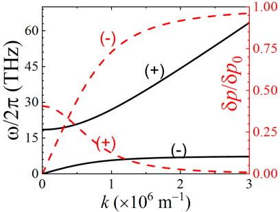
Figure 2: The dispersion relations (solid black curves) and the corresponding electric dipoles (dashed red curves) of two $(\pm)$ of ferron polaritons branches in the absence of damping. The electric dipoles are normalized by the value at the origin $\delta p_{0}=-0.15$ eÅ. The parameters are for LiNbO₃ with $\varepsilon(\infty)=5.5$.

Electric dipole of ferron polaritons. Photons can hybridize with optical phonons to form phonon polaritons  Born et al. (1955); Fano (1956); Henry and Hopfield (1965); Bakker et al. (1992); Kojima et al. (2002, 2003); Ikegaya et al. (2015), that can show anharmonicities in ferroelectrics Bakker et al. (1994, 1998). We may therefore consider “ferron polaritons” with a dispersion relation governed by Born et al. (1955)

$$\frac{c^{2}k^{2}}{\omega^{2}}=\varepsilon(\omega)$$ (51)

where $c$, $k$ and $\varepsilon(\omega)$ are the light velocity, wave vector and the dynamic (relative) permittivity in the long-wavelength limit, respectively. According to Eq. (7)

$$\varepsilon(\omega)-\varepsilon(\infty)\equiv\frac{\delta P_{\mathrm{h}}}{\varepsilon_{0}E_{\mathrm{th}}}=\frac{1}{m_{p}\varepsilon_{0}(\omega_{0}^{2}-\omega^{2}-i\omega\tilde{\gamma})}$$ (52)

where $\tilde{\gamma}=\gamma/m_{p}$, while $\varepsilon(\infty)$ is the high-frequency permittivity. While this dispersion is identical to that of the phonon polaritons in normal ionic crystals Born et al. (1955); Fano (1956), the ferron polaritons may transport electric dipoles below $T_{c}$. By Eq. (12), the electric dipole of ferron polaritons reads

$$\delta p_{\pm}(k)=-\left.\frac{\partial\hbar\omega_{\pm}(k)}{\partial E}\right|_{E\rightarrow 0}=\frac{\partial\omega_{\pm}(k)}{\partial\omega_{0}}\delta p_{0}$$ (53)

where $+(-)$ indicates two (optical and ferronic) branches and $\delta p_{0}=-\partial\hbar\omega_{0}/\partial E$. Figure 2 gives the dispersion relations and the electric dipoles carried by the two branches for LiNbO₃, in which the level repulsion renders the dipole of the ferronic branch smaller than $\delta p_{0}$ even at $k=0$. Focused optical excitations at the optical phonon frequency of ferroelectrics can therefore be a source of coherent polarization currents and give rise to unique electrooptic properties such as electric field-controlled light propagation. Electric-dipolar interaction importantly affects the surface ferron-polariton dispersion relations Rezende and Rodríguez-Suárez .

Conclusions: We identify the quasi-particle excitations of displacive ferroelectrics that carry heat and electric dipole currents and predict the associated low-temperature pyroelectric or electrocaloric coefficients, the (field-dependent) thermal conductivity, Peltier and Seebeck coefficients, and ferron polariton polarization. Thermally driven and electrically tunable ferronic transport in a broad class of ferroelectric materials may provide unique functionalities to thermal management and information technologies.

Acknowledgements: We are grateful for enlightening discussions with Beatriz Noheda, Bart J. van Wees, Joseph P. Heremans, and Sergio Rezende. JSPS KAKENHI Grant No. 19H00645 supported P.T. and G.B. R.I. and K.U. acknowledge support by JSPS KAKENHI Grant No. 20H02609, JST CREST “Creation of Innovative Core Technologies for Nano-enabled Thermal Management”Grant No. JPMJCR17I1, and the Canon Foundation.

References

- Kruglyak et al. (2010) V. V. Kruglyak, S. O. Demokritov, and D. Grundler, Journal of Physics D: Applied Physics 43, 264001 (2010).
- Chumak et al. (2015) A. V. Chumak, V. I. Vasyuchka, A. A. Serga, and B. Hillebrands, Nature Physics 11, 453 (2015).
- Cornelissen et al. (2015) L. J. Cornelissen, J. Liu, R. A. Duine, J. B. Youssef, and B. J. van Wees, Nature Physics 11, 1022 (2015).
- Cornelissen et al. (2016) L. J. Cornelissen, K. J. Peters, G. E. Bauer, R. A. Duine, and B. J. van Wees, Physical Review B 94, 014412 (2016).
- Uchida et al. (2010) K.-i. Uchida, J. Xiao, H. Adachi, J.-i. Ohe, S. Takahashi, J. Ieda, T. Ota, Y. Kajiwara, H. Umezawa, H. Kawai, G. E. W. Bauer, M. S., and S. E., Nature Materials 9, 894 (2010).
- Flipse et al. (2014) J. Flipse, F. K. Dejene, D. Wagenaar, G. E. W. Bauer, J. B. Youssef, and B. J. Van Wees, Physical Review Letters 113, 027601 (2014).
- Daimon et al. (2016) S. Daimon, R. Iguchi, T. Hioki, E. Saitoh, and K.-i. Uchida, Nature Communications 7, 1 (2016).
- Xu (2013) Y. Xu, Ferroelectric materials and their applications (Elsevier, 2013).
- Spaldin (2007) N. A. Spaldin, Top. Appl. Phys. 105, 175 (2007).
- Bauer et al. (2021) G. E. W. Bauer, R. Iguchi, and K.-i. Uchida, Physical Review Letters 126, 187603 (2021).
- Tang et al. (2021) P. Tang, R. Iguchi, K.-i. Uchida, and G. E. W. Bauer, Physical Review Letters 128 (2021).
- Blinc and Žekš (1972) R. Blinc and B. Žekš, Advances in Physics 21, 693 (1972).
- Cochran (1959) W. Cochran, Physical Review Letters 3, 412 (1959).
- Cochran (1960) W. Cochran, Advances in Physics 9, 387 (1960).
- Müller et al. (1982) K. Müller, Y. Luspin, J. Servoin, and F. Gervais, Journal de Physique Lettres 43, 537 (1982).
- Dalal et al. (1998) N. Dalal, A. Klymachyov, and A. Bussmann-Holder, Physical Review Letters 81, 5924 (1998).
- Zalar et al. (2003) B. Zalar, V. V. Laguta, and R. Blinc, Physical Review Letters 90, 037601 (2003).
- Bussmann-Holder et al. (2009) A. Bussmann-Holder, H. Beige, and G. Völkel, Physical Review B 79, 184111 (2009).
- Devonshire (1949) A. F. Devonshire, The London, Edinburgh, and Dublin Philosophical Magazine and Journal of Science 40, 1040 (1949).
- Devonshire (1951) A. Devonshire, The London, Edinburgh, and Dublin Philosophical Magazine and Journal of Science 42, 1065 (1951).
- Salje (1990) E. Salje, Ferroelectrics 104, 111 (1990).
- Cao (2008) W. Cao, Ferroelectrics 375, 28 (2008).
- Chandra and Littlewood (2007) P. Chandra and P. B. Littlewood, Physics of Ferroelectrics , 69 (2007).
- Tani (1969) K. Tani, Journal of the Physical Society of Japan 26, 93 (1969).
- Ishibashi (1989) Y. Ishibashi, Ferroelectrics 98, 193 (1989).
- Sivasubramanian et al. (2004) S. Sivasubramanian, A. Widom, and Y. N. Srivastava, Ferroelectrics 300, 43 (2004).
- Widom et al. (2010) A. Widom, S. Sivasubramanian, C. Vittoria, S. Yoon, and Y. N. Srivastava, Physical Review B 81, 212402 (2010).
- Landau et al. (1980) L. D. Landau, E. M. Lifshitz, and L. P. Pitaevskii, Statistical Physics, Part 1, 3rd ed (Pergamon, New York, 1980).
- Tadano and Tsuneyuki (2018) T. Tadano and S. Tsuneyuki, Journal of the Physical Society of Japan 87, 041015 (2018).
- (30) P. Tang and G. Bauer, unpublished .
- Haun et al. (1987) M. J. Haun, E. Furman, S. Jang, H. McKinstry, and L. Cross, Journal of Applied Physics 62, 3331 (1987).
- Pertsev et al. (1998) N. Pertsev, A. Zembilgotov, and A. Tagantsev, Physical Review Letters 80, 1988 (1998).
- Scrymgeour et al. (2005) D. A. Scrymgeour, V. Gopalan, A. Itagi, A. Saxena, and P. J. Swart, Physical Review B 71, 184110 (2005).
- Li et al. (2005) Y. Li, L. Cross, and L. Chen, Journal of Applied Physics 98, 064101 (2005).
- Hlinka and Marton (2006) J. Hlinka and P. Marton, Physical Review B 74, 104104 (2006).
- Liang et al. (2009) L. Liang, Y. Li, L.-Q. Chen, S. Hu, and G.-H. Lu, Applied Physics Letters 94, 072904 (2009).
- Whatmore (1986) R. Whatmore, Reports on Progress in Physics 49, 1335 (1986).
- Muralt (2001) P. Muralt, Reports on Progress in Physics 64, 1339 (2001).
- Mischenko et al. (2006) A. Mischenko, Q. Zhang, J. Scott, R. Whatmore, and N. Mathur, Science 311, 1270 (2006).
- Neese et al. (2008) B. Neese, B. Chu, S.-G. Lu, Y. Wang, E. Furman, and Q. Zhang, Science 321, 821 (2008).
- Li et al. (2020) X. Li, S.-G. Lu, X.-Z. Chen, H. Gu, X.-s. Qian, and Q. Zhang, in Progress in Advanced Dielectrics (World Scientific, 2020) pp. 329–367.
- Glass and Lines (1976) A. Glass and M. Lines, Physical Review B 13, 180 (1976).
- Lang et al. (1969) S. B. Lang, L. H. Rice, and S. A. Shaw, Journal of Applied Physics 40, 4335 (1969).
- Born (1945) M. Born, Reviews of Modern Physics 17, 245 (1945).
- Szigeti (1975) B. Szigeti, Physical Review Letters 35, 1532 (1975).
- Bauer et al. (2022) G. E. W. Bauer, P. Tang, R. Iguchi, and K. Uchida, Journal of Magnetism and Magnetic Materials 541, 168468 (2022).
- Behera et al. (2011) R. K. Behera, C.-W. Lee, D. Lee, A. N. Morozovska, S. B. Sinnott, A. Asthagiri, V. Gopalan, and S. R. Phillpot, Journal of Physics: Condensed Matter 23, 175902 (2011).
- Richman et al. (2019) M. S. Richman, X. Li, and A. Caruso, Journal of Applied Physics 125, 184103 (2019).
- Morozovska et al. (2016) A. N. Morozovska, E. A. Eliseev, C. M. Scherbakov, and Y. M. Vysochanskii, Physical Review B 94, 174112 (2016).
- (50) was estimated from the broadening () of the lowest A1(TO) line in Raman-scattering spectra .
- Fontana et al. (1994) M. Fontana, K. Laabidi, and B. Jannot, Journal of Physics: Condensed Matter 6, 8923 (1994).
- Sanjurjo et al. (1983) J. Sanjurjo, E. Lopez-Cruz, and G. Burns, Physical Review B 28, 7260 (1983).
- Ridah et al. (1997) A. Ridah, M. Fontana, and P. Bourson, Physical Review B 56, 5967 (1997).
- Suemune (1965) Y. Suemune, Journal of the Physical Society of Japan 20, 174 (1965).
- Langenberg et al. (2019) E. Langenberg, D. Saha, M. E. Holtz, J.-J. Wang, D. Bugallo, E. Ferreiro-Vila, H. Paik, I. Hanke, S. Ganschow, D. A. Muller, et al., Nano Letters 19, 7901 (2019).
- Burkhart and Rice (1977) G. Burkhart and R. Rice, Journal of Applied Physics 48, 4817 (1977).
- (57) J. Heremans, unpublished experiment .
- Mante and Volger (1971) A. Mante and J. Volger, Physica 52, 577 (1971).
- Northrop et al. (1982) G. Northrop, E. Cotts, A. Anderson, and J. Wolfe, Physical Review Letters 49, 54 (1982).
- Weilert et al. (1993) M. Weilert, M. Msall, J. Wolfe, and A. Anderson, Zeitschrift für Physik B Condensed Matter 91, 179 (1993).
- Born et al. (1955) M. Born, K. Huang, and M. Lax, American Journal of Physics 23, 474 (1955).
- Fano (1956) U. Fano, Physical Review 103, 1202 (1956).
- Henry and Hopfield (1965) C. Henry and J. Hopfield, Physical Review Letters 15, 964 (1965).
- Bakker et al. (1992) H. Bakker, S. Hunsche, and H. Kurz, Physical Review Letters 69, 2823 (1992).
- Kojima et al. (2002) S. Kojima, N. Tsumura, H. Kitahara, M. W. Takeda, and S. Nishizawa, Japanese Journal of Applied Physics 41, 7033 (2002).
- Kojima et al. (2003) S. Kojima, N. Tsumura, M. W. Takeda, and S. Nishizawa, Physical Review B 67, 035102 (2003).
- Ikegaya et al. (2015) Y. Ikegaya, H. Sakaibara, Y. Minami, I. Katayama, and J. Takeda, Applied Physics Letters 107, 062901 (2015).
- Bakker et al. (1994) H. Bakker, S. Hunsche, and H. Kurz, Physical Review B 50, 914 (1994).
- Bakker et al. (1998) H. Bakker, S. Hunsche, and H. Kurz, Reviews of Modern Physics 70, 523 (1998).
- (70) S. M. Rezende and R. L. Rodríguez-Suárez, unpublished .