Reconfigurable MIMO towards Electro-magnetic Information Theory: Capacity Maximization Pattern Design

Abstract

In this paper, we focus on the pattern reconfigurable multiple-input multiple-output (PR-MIMO), a technique that has the potential to bridge the gap between electro-magnetics and communications towards the emerging Electro-magnetic Information Theory (EIT). Specifically, we focus on the pattern design problem aimed at maximizing the channel capacity for reconfigurable MIMO communication systems, where we firstly introduce the matrix representation of PR-MIMO and further formulate a pattern design problem. We decompose the pattern design into two steps, i.e., the correlation modification process to optimize the correlation structure of the channel, followed by the power allocation process to improve the channel quality based on the optimized channel structure. For the correlation modification process, we propose a sequential optimization framework with eigenvalue decomposition to obtain near-optimal solutions. For the power allocation process, we provide a closed-form power allocation scheme to redistribute the transmission power among the modified subchannels. Numerical results show that the proposed pattern design scheme offers significant improvements over legacy MIMO systems, which motivates the application of PR-MIMO in wireless communication systems.

I Introduction

During the past decades, Multiple-Input Multiple-Output (MIMO) technology has shown its great potential in improving the performance of wireless communication systems because of the ability to exploit the spatial resource over single-antenna systems [1]. Nevertheless, the capacity of modern MIMO communication systems have shown to approach the Shannon limits. To meet the ever-increasing demand for data rates in 5.5G/6G and beyond, the concept of Electromagnetic Information Theory (EIT) has recently been proposed [2], which aims to merge the electro-magnetics and information theory that have been studied separately for years. Pattern reconfigurable MIMO (PR-MIMO) based on reconfigurable antennas is able to affect the electro-magnetic fields via reconfiguring the radiation pattern, which has the potential to bridge the gap between electro-magnetics and information theory [3].

Based on the advances on antenna design techniques, reconfigurable antennas can be designed to operate with different radiation characteristics, such as frequency bands, polarizations or radiation patterns [4, 5]. Compared with other reconfigurable dimensions, the pattern reconfigurability, which is mainly discussed in this paper, can further enhance the ability of interference cancellation and resource allocation by improving the degrees of freedom (DoFs). PR-MIMO can offer spatial diversity in radiation directivity at the same transmission frequency, and a great quantity of methods have been studied to realize PR-MIMO [6], such as switching the circuit [7, 8], choosing different radiation units, etc. [9, 10, 11].

The applications of PR-MIMO in practical wireless scenarios such as user scheduling [12], target location [13], direction of arrival (DoA) estimation [14, 15], have been discussed recently. In [12], PR-MIMO improved the performance by expanding the users scheduling region via the additional reconfigurable channels. The pairing scheduling was determined by the proposed joint user and antenna mode selection scheme, and a greedy low-complexity iterative selection algorithm was further designed. [13] considered PR-MIMO for target detection and tracking, where a Bayesian cognitive target tracking technique to minimize the Cramér-Rao lower bound (CRLB) of the DoA parameters was proposed. Considering the DoA estimation for PR-MIMO, [14] and [15] combined the traditional methods with the adaptive decision algorithm and further improved the estimation accuracy.

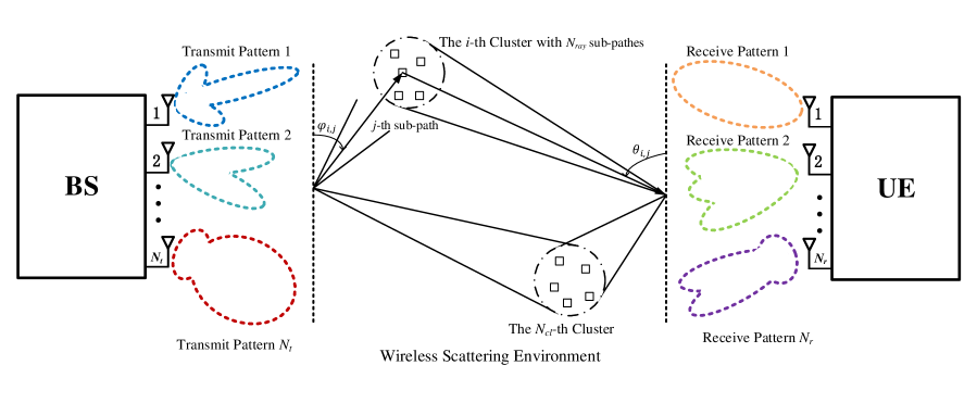
Figure 1: Multi-path channel model for PR-MIMO.

However, two challenges that hinder the widely application of PR-MIMO still exist. On one hand, the exploitation of the additional DoFs has to be accomplished through the effective optimal mode selection, which brings considerable channel estimation overhead. The channel extrapolation based on the pattern correlation [16] and the optimal decision algorithm based on Multi-Armed Bandit (MAB) [17, 18, 19, 20, 21] are the major attempts to solve this problem currently. Moreover, the physical mechanism of the modification process and the quality improvement in PR-MIMO has not been revealed, and the methodology of the radiation pattern design in PR-MIMO systems for optimizing some wireless performance metrics such as capacity maximization has not been established.

In this paper, we study the pattern design problem aimed at maximizing the channel capacity for PR-MIMO systems. We firstly describe the pattern channel in a matrix form and further formulate a pattern design optimization problem. After revealing the physical mechanism of the pattern effect on the scattering channel, we decompose the optimal pattern design into two steps, i.e., the correlation modification process to optimize the correlation structure of the channel, and the power allocation process to improve the channel quality, sequentially. For the correlation modification process, we propose a sequential optimization framework (SOF) to transform the correlation modification matrix design problem into a sequential vector optimization problems, which can be solved using eigenvalue decomposition based method, and give a criterion to determine their optimized sequences. For the power allocation process, a closed-form scheme is designed to redistribute the transmission power according to the independence level of the subchannels. Numerical results demonstrate the efficient channel modification ability of the designed reconfigurable pattern and further validate the significant improvements of PR-MIMO over legacy MIMO systems.

Notations: $a$, $\boldsymbol{a}$, and $\mathbf{A}$ denote scalar, column vector and matrix, respectively. $(\cdot)^{*}$, $(\cdot)^{\mathrm{T}}$, and $(\cdot)^{\mathrm{H}}$ denote conjugate, transposition, conjugate transposition respectively while $\operatorname{Tr}\left(\cdot\right)$ represents the trace of a matrix. $\operatorname{vec}\left(\cdot\right)$ denotes the vectorization operator and $\operatorname{diag}\left(\cdot\right)$ denotes the diagonalization operator. $\left\langle\cdot\right\rangle$ denotes the inner product operation, i.e., $\left\langle\boldsymbol{a},\boldsymbol{b}\right\rangle=\boldsymbol{a}^{\mathrm{H}}\boldsymbol{b}$ for complex vectors $\boldsymbol{a}$ and $\boldsymbol{b}$. Frobenius norm of a matrix is denoted by $\|\cdot\|_{\mathrm{F}}$. $\mathbf{I}_{M}$ and $\mathbf{1}_{M\times N}$ represent a $M\times M$ identity matrix and a $M\times N$ with all entries being $1$. $\mathcal{S}_{L}$ denotes all $L\times L$ symmetric matrices. $\boldsymbol{e}_{i}$ is the $i$-th column of an identity matrix. $\succeq$ and $\preceq$ represent matrix generalized inequalities. $\odot$ denotes Hadamard product.

II System Model

In this section, we firstly present the multi-path channel model and the pattern reconfigurable channel model. After that, the capacity of PR-MIMO is introduced.

II-A Multi-Path MIMO Channel Model

We consider a point-to-point (P2P) MIMO system in the downlink, equipped with $N_{t}$ antennas at the transmitter and $N_{r}$ antennas at the receiver, where $N_{r}\leq N_{t}$, as shown in Fig. 1. Assuming the uniform linear array (ULA) at the transceivers, the physical multi-path MIMO channel can be modeled as [22]:

$$\mathbf{H}=\sum_{l=1}^{L}\alpha_{l}\boldsymbol{a}_{\mathrm{R}}\left(\theta_{l}\right)\boldsymbol{a}_{\mathrm{T}}^{\mathrm{H}}\left(\varphi_{l}\right),$$ (1)

where $\mathbf{H}\in\mathbb{C}^{N_{r}\times N_{t}}$ represents the channel matrix with the power constraint $\mathbb{E}\left[\|\mathbf{H}\|_{\mathrm{F}}^{2}\right]=N_{t}N_{r}$, $L$ is the scattering paths number and $\alpha_{l}$ denotes the channel gain of the $l$-th scattering path. The steering vectors at the receiver and the transmitter are given by

$$\boldsymbol{a}_{\mathrm{R}}\left(\theta_{l}\right)=\dfrac{1}{\sqrt{N_{r}}}\left[1,e^{-j2\pi\frac{d_{\mathrm{R}}}{\lambda}\sin\theta_{l}},\ldots,e^{-j2\pi\frac{d_{\mathrm{R}}}{\lambda}\left(N_{r}-1\right)\sin\theta_{l}}\right]^{\mathrm{T}}$$ (2)

and

$$\boldsymbol{a}_{\mathrm{T}}\left(\varphi_{l}\right)=\dfrac{1}{\sqrt{N_{t}}}\left[1,e^{-j2\pi\frac{d_{\mathrm{T}}}{\lambda}\sin\varphi_{l}},\ldots,e^{-j2\pi\frac{d_{\mathrm{T}}}{\lambda}\left(N_{t}-1\right)\sin\varphi_{l}}\right]^{\mathrm{T}},$$ (3)

where $\frac{d_{\mathrm{T}}}{\lambda}$ and $\frac{d_{\mathrm{R}}}{\lambda}$ represent the normalized antenna spacing at the transceivers, with the carrier wavelength $\lambda$. $\theta_{l}$ and $\varphi_{l}$ denote the azimuth angles of arrival and departure (AoAs and AoDs). Based on that, (1) can be simplified into

$$\mathbf{H}=\mathbf{A}_{\mathrm{R}}\mathbf{\Lambda}\mathbf{A}_{\mathrm{T}}^{\mathrm{H}},$$ (4)

where

$$\mathbf{A}_{\mathrm{R}}=\left[\boldsymbol{a}_{\mathrm{R}}\left(\theta_{1}\right),\boldsymbol{a}_{\mathrm{R}}\left(\theta_{2}\right),\ldots,\boldsymbol{a}_{\mathrm{R}}\left(\theta_{L}\right)\right]$$ (5)

and

$$\mathbf{A}_{\mathrm{T}}=\left[\boldsymbol{a}_{\mathrm{T}}\left(\varphi_{1}\right),\boldsymbol{a}_{\mathrm{T}}\left(\varphi_{2}\right),\ldots,\boldsymbol{a}_{\mathrm{T}}\left(\varphi_{L}\right)\right]$$ (6)

are the steering matrices of the transceivers, and $\mathbf{\Lambda}=\operatorname{diag}\left\{\alpha_{1},\alpha_{2},\ldots,\alpha_{L}\right\}$ contains the complex channel gains on the diagonal.

Considering that the channel model $\mathbf{H}$ only describes the physical scattering information without the antenna radiation characteristics, we term it the physical channel.

II-B PR-MIMO Channel Model

$$\widetilde{\mathbf{H}}= \sum_{l=1}^{L}\alpha_{l}\boldsymbol{a}_{\mathrm{R}}\left(\theta_{l}\right)\boldsymbol{a}_{\mathrm{T}}^{\mathrm{H}}\left(\varphi_{l}\right)\odot\left({\left[\begin{array}[]{cl}F_{\mathrm{v},\theta_{l},v_{1}}^{\mathrm{Re}}&F_{\mathrm{h},\vartheta_{l},v_{1}}^{\mathrm{Re}}\\ F_{\mathrm{v},\theta_{l},v_{2}}^{\mathrm{Re}}&F_{\mathrm{h},\vartheta_{l},v_{2}}^{\mathrm{Re}}\\ \vdots&\vdots\\ F_{\mathrm{v},\theta_{l},v_{N_{r}}}^{\mathrm{Re}}&F_{\mathrm{h},\vartheta_{l},v_{N_{r}}}^{\mathrm{Re}}\end{array}\right]}\left[\begin{array}[]{llll}F_{\mathrm{v},\varphi_{l},\mu_{1}}^{\mathrm{Tr}}&F_{\mathrm{v},\varphi_{l},\mu_{2}}^{\mathrm{Tr}}&\ldots&F_{\mathrm{v},\varphi_{l},\mu_{N_{t}}}^{\mathrm{Tr}}\\ \\ F_{\mathrm{h},\phi_{l},\mu_{1}}^{\mathrm{Tr}}&F_{\mathrm{h},\phi_{l},\mu_{2}}^{\mathrm{Tr}}&\ldots&F_{\mathrm{h},\phi_{l},\mu_{N_{t}}}^{\mathrm{Tr}}\end{array}\right]\right).$$ (9)

$$\widetilde{\mathbf{H}}= \sum_{l=1}^{L}\alpha_{l}\boldsymbol{a}_{\mathrm{R}}\left(\theta_{l}\right)\boldsymbol{a}_{\mathrm{T}}^{\mathrm{H}}\left(\varphi_{l}\right)\odot\left[\begin{array}[]{cccc}F_{\mathrm{v},\varphi_{l},\mu_{1}}^{\mathrm{Tr}}&F_{\mathrm{v},\varphi_{l},\mu_{2}}^{\mathrm{Tr}}&\cdots&F_{\mathrm{v},\varphi_{l},\mu_{N_{t}}}^{\mathrm{Tr}}\\ F_{\mathrm{v},\varphi_{l},\mu_{1}}^{\mathrm{Tr}}&F_{\mathrm{v},\varphi_{l},\mu_{2}}^{\mathrm{Tr}}&\cdots&F_{\mathrm{v},\varphi_{l},\mu_{N_{t}}}^{\mathrm{Tr}}\\ \vdots&\ddots&\vdots&\vdots\\ F_{\mathrm{v},\varphi_{l},\mu_{1}}^{\mathrm{Tr}}&F_{\mathrm{v},\varphi_{l},\mu_{2}}^{\mathrm{Tr}}&\cdots&F_{\mathrm{v},\varphi_{l},\mu_{N_{t}}}^{\mathrm{Tr}}\end{array}\right]$$ (11)

$$= \mathbf{A}_{\mathrm{R}}\mathbf{\Lambda}\left(\mathbf{A}_{\mathrm{T}}\odot\left[\begin{array}[]{cccc}F_{\mathrm{v},\varphi_{1},\mu_{1}}^{\mathrm{Tr}}&F_{\mathrm{v},\varphi_{2},\mu_{1}}^{\mathrm{Tr}}&\cdots&F_{\mathrm{v},\varphi_{L},\mu_{1}}^{\mathrm{Tr}}\\ F_{\mathrm{v},\varphi_{1},\mu_{2}}^{\mathrm{Tr}}&F_{\mathrm{v},\varphi_{2},\mu_{2}}^{\mathrm{Tr}}&\cdots&F_{\mathrm{v},\varphi_{L},\mu_{2}}^{\mathrm{Tr}}\\ \vdots&\ddots&\vdots&\vdots\\ F_{\mathrm{v},\varphi_{1},\mu_{N_{t}}}^{\mathrm{Tr}}&F_{\mathrm{v},\varphi_{2},\mu_{N_{t}}}^{\mathrm{Tr}}&\cdots&F_{\mathrm{v},\varphi_{L},\mu_{N_{t}}}^{\mathrm{Tr}}\end{array}\right]\right)^{\mathrm{H}},$$

$$= \mathbf{A}_{\mathrm{R}}\mathbf{\Lambda}\left(\mathbf{A}_{\mathrm{T}}\odot\mathbf{M}\right)^{\mathrm{H}}.$$

Considering pattern reconfigurable antennas at both the transceivers, the complex channel gain between the $m$-th transmit antenna and the $n$-th receive antenna is represented as [16]

$$\widetilde{\mathbf{H}}_{n,m}\left(\mu_{m},v_{n}\right)=\sum_{l=1}^{L}\alpha_{l} \left\langle\vec{f}_{\mathrm{T}}\left(\varphi_{l},\phi_{l},\mu_{m}\right),\vec{f}_{\mathrm{R}}\left(\theta_{l},\vartheta_{l},v_{n}\right)\right\rangle$$ (7)

$$e^{j2\pi\left(\frac{d_{\mathrm{T}}}{\lambda}(m-1)\sin\varphi_{l}-\frac{d_{\mathrm{R}}}{\lambda}(n-1)\sin\theta_{l}\right)},$$

where $\vec{f}_{\mathrm{T}}\left(\varphi_{l},\phi_{l},\mu_{m}\right)=\left[F_{\mathrm{v},\varphi_{l},\mu_{m}}^{\mathrm{Tr}},F_{\mathrm{h},\phi_{l},\mu_{m}}^{\mathrm{Tr}}\right]^{\mathrm{T}}$ and $\vec{f}_{\mathrm{R}}\left(\theta_{l},\vartheta_{l},v_{n}\right)=\left[F_{\mathrm{v},\theta_{l},v_{n}}^{\mathrm{Re}},F_{\mathrm{h},\vartheta_{l},v_{n}}^{\mathrm{Re}}\right]^{\mathrm{T}}$ are the electric pattern vectors of the $m$-th transmit antenna with pattern $\mu_{m}$ and the $n$-th receive antenna with pattern $v_{n}$ in the direction of $\mathrm{AoD}=\varphi_{l}$, $\mathrm{EoD}=\phi_{l}$, $\mathrm{AoA}=\theta_{l}$ and $\mathrm{EoA}=\vartheta_{l}$, where $\mathrm{EoD}$ and $\mathrm{EoA}$ are abbreviations for elevation angle of departure and that of arrival, while $\mathrm{AoD}$ and $\mathrm{AoA}$ are abbreviations for azimuth angle of departure and that of arrival, respectively. $F_{\mathrm{v}}$ and $F_{\mathrm{h}}$ denote the projection of the pattern vector on the vertical and horizontal dimensions. According to (7), the inner product of the pattern vectors describes the modification process of the antenna pattern. Similarly, we term $\widetilde{\mathbf{H}}$ the pattern channel matrix.

$$\mathcal{P}_{1}:\max_{\mathbf{M}} \log_{2}\operatorname{det}\left({\mathbf{I}_{N_{r}}+\frac{\rho}{N_{r}}\mathbf{A}_{\mathrm{R}}\mathbf{\Lambda}\left(\mathbf{A}_{\mathrm{T}}\odot\mathbf{M}\right)^{\mathrm{H}}}{\left(\mathbf{A}_{\mathrm{T}}\odot\mathbf{M}\right)\mathbf{\Lambda}^{\mathrm{H}}\mathbf{A}_{\mathrm{R}}^{\mathrm{H}}}\right)$$ (12)

s.t. $$\operatorname{Tr}\left(\mathbf{A}_{\mathrm{R}}\mathbf{\Lambda}\left(\mathbf{A}_{\mathrm{T}}\odot\mathbf{M}\right)^{\mathrm{H}}\left(\mathbf{A}_{\mathrm{T}}\odot\mathbf{M}\right)\mathbf{\Lambda}^{\mathrm{H}}\mathbf{A}_{\mathrm{R}}^{\mathrm{H}}\right)\leq N_{r}N_{t},$$

$$\mathbf{M}_{i,j}\geq 0\quad i,j=1,2,\ldots,L.$$

$$\widehat{\mathbf{G}}_{i,j} =\operatorname{Tr}\left(\widehat{\mathbf{H}}_{i}^{\mathrm{H}}\widehat{\mathbf{H}}_{j}\right)$$ (16)

$$=\operatorname{Tr}\left(\left(\boldsymbol{a}_{\mathrm{T},i}\odot\widehat{\boldsymbol{m}}_{i}\right)\boldsymbol{a}_{\mathrm{R},i}^{\mathrm{H}}\boldsymbol{a}_{\mathrm{R},j}\left(\boldsymbol{a}_{\mathrm{T},j}\odot\widehat{\boldsymbol{m}}_{j}\right)^{\mathrm{H}}\right)$$

$$=\frac{1}{N_{r}N_{t}}\sum_{n=1}^{N_{r}}e^{j2\pi\frac{d_{\mathrm{R}}}{\lambda}(n-1)\left(\sin\theta_{j}-\sin\theta_{i}\right)}\sum_{k=1}^{N_{t}}\widehat{\boldsymbol{m}}_{i}(k)\widehat{\boldsymbol{m}}_{j}(k)e^{j2\pi\frac{d_{\mathrm{T}}}{\lambda}(k-1)\left(\sin\varphi_{i}-\sin\varphi_{j}\right)}.$$

II-C Capacity of PR-MIMO

Assuming that the transmitter holds the perfect channel state information, the capacity for a PR-MIMO system is given by

$$C=\log_{2}\operatorname{det}\left(\mathbf{I}_{N_{r}}+\frac{\rho}{N_{r}}\widetilde{\mathbf{H}}\widetilde{\mathbf{H}}^{\mathrm{H}}\right),$$ (8)

where $\rho$ represents the transmit signal-to-noise ratio (SNR).

III Problem Formulation

In this section, we firstly discuss how to describe the pattern channel in a matrix form, based on which the pattern design problem is further formulated.

III-A Matrix Representation of PR-MIMO

Firstly, the reason to describe the pattern channel in a matrix form should be explained. The element-wise channel representation in (7) only describes the mathematical generation process of the pattern channel, but cannot reveal the physical mechanism of the pattern effect. The optimal pattern design calls for a matrix representation of the PA-MIMO channel.

The expansion of the matrix form is shown in (9) at the bottom of this page. Considering the transmit pattern reconfigurability only in this paper for simplicity, the receiver pattern is given by

$$\left[\begin{array}[]{cc}F_{\mathrm{v},\theta_{l},v_{1}}^{\mathrm{Re}}&F_{\mathrm{h},\vartheta_{l},v_{1}}^{\mathrm{Re}}\\ F_{\mathrm{v},\theta_{l},v_{2}}^{\mathrm{Re}}&F_{\mathrm{h},\vartheta_{l},v_{2}}^{\mathrm{Re}}\\ \vdots&\vdots\\ F_{\mathrm{v},\theta_{l},v_{N_{r}}}^{\mathrm{Re}}&F_{\mathrm{h},\vartheta_{l},v_{N_{r}}}^{\mathrm{Re}}\end{array}\right]=\left[\begin{array}[]{cc}1&0\\ 1&0\\ \vdots&\vdots\\ 1&0\end{array}\right].$$ (10)

where only the vertical polarization is considered. Based on that, (9) can be further simplified into (11) at the bottom of this page.

According to (11), the reconfigurable pattern modifies the channel via introducing an extra power factor in the corresponding transmission direction. The pattern sampling matrix $\mathbf{M}$ in (11), whose $(k,l)$-th element denotes the sampling radiation pattern gain of the $k$-th antenna element in the $l$-th scattering direction, reveals the physical mechanism of pattern modification and motivates us to formulate the pattern design problem, as shown in the following.

III-B Problem Formulation

The capacity maximization pattern design problem can be constructed as $\mathcal{P}_{1}$ in (12) at the bottom of this page. The first constraint prevents the additional power gain, while the second one enforces that only the power modification effect of the pattern is considered, without the phase adjustment ability. Considering that all the antenna elements are equipped with the same reconfigurable pattern such that $\operatorname{rank}\left(\mathbf{M}\right)=1$, $\mathcal{P}_{1}$ can be further transformed into

$$\mathcal{P}_{2}:\min_{\mathbf{X}} -\log_{2}\operatorname{det}\left(\mathbf{I}_{N_{r}}+\frac{\rho}{N_{r}}\mathbf{A}_{\mathrm{R}}\mathbf{\Lambda}\left(\mathbf{R}_{\mathrm{T}}\odot\mathbf{X}\right)\mathbf{\Lambda}^{\mathrm{H}}\mathbf{A}_{\mathrm{R}}^{\mathrm{H}}\right)$$ (13)

s.t. $$\operatorname{Tr}\left(\mathbf{A}_{\mathrm{R}}\mathbf{\Lambda}\left(\mathbf{R}_{\mathrm{T}}\odot\mathbf{X}\right)\mathbf{\Lambda}^{\mathrm{H}}\mathbf{A}_{\mathrm{R}}^{\mathrm{H}}\right)\leq N_{r}N_{t},$$

$$\mathbf{X}\in\mathcal{C}_{L},\ \operatorname{rank}\left(\mathbf{X}\right)=1$$

where $\mathbf{X}=\mathbf{M}^{\mathrm{T}}\mathbf{M}$ is the covariance matrix of $\mathbf{M}$ and $\mathcal{C}_{L}$ defines the closed convex cone of completely positive (CP) matrices, whose definition is shown as below [23]

$$\mathcal{C}_{L}:=\left\{\mathbf{X}\in\mathcal{S}_{L}:\mathbf{X}=\mathbf{N}\mathbf{N}^{\mathrm{T}}\text{ for some }\mathbf{N}\geqslant 0\right\},$$ (14)

where $\mathbf{X}\succeq 0$ denotes a positive semidifinite matrix and $\mathbf{X}\geqslant 0$ denotes an entry-wise nonnegative matrix.

IV Proposed Pattern Design Algorithm

In this section, we firstly show that the capacity maximization pattern design can be decomposed into the correlation modification process and the power allocation process. Subsequently, the sequential optimization framework and the closed-form power allocation scheme are proposed for each process.

Firstly, (11) can be further transformed into

$$\widetilde{\mathbf{H}} =\mathbf{A}_{\mathrm{R}}\mathbf{\Lambda}\left(\mathbf{A}_{\mathrm{T}}\odot\mathbf{M}\right)^{\mathrm{H}}$$ (15)

$$=\sum_{i=1}^{L}\alpha_{i}\boldsymbol{a}_{\mathrm{R},i}\left(\boldsymbol{a}_{\mathrm{T},i}\odot\mathbf{M}(:,i)\right)^{\mathrm{H}}$$

$$=\sum_{i=1}^{L}\alpha_{i}p_{i}\boldsymbol{a}_{\mathrm{R},i}\left(\boldsymbol{a}_{\mathrm{T},i}\odot\widehat{\boldsymbol{m}}_{i}\right)^{\mathrm{H}}=\sum_{i=1}^{L}\alpha_{i}p_{i}\widehat{\mathbf{H}}_{i},$$

where $\widehat{\mathbf{H}}_{i}=\boldsymbol{a}_{\mathrm{R},i}\left(\boldsymbol{a}_{\mathrm{T},i}\odot\widehat{\boldsymbol{m}}_{i}\right)^{\mathrm{H}}$ is the $i$-th normalized modified subchannel. According to (15), the modification effect on the $i$-th scattering subchannel is accomplished via the correlation modification vector $\widehat{\boldsymbol{m}}_{i}=\frac{1}{p_{i}}\mathbf{M}(:,i)$ with $\left\|\widehat{\boldsymbol{m}}_{i}\right\|_{2}^{2}=N_{t}$, and the power allocation factor $p_{i}$.

From (15), the capacity maximization pattern design can be decomposed into two steps. Firstly, the correlation modification matrix $\widehat{\mathbf{M}}=\left[\widehat{\boldsymbol{m}}_{1},\widehat{\boldsymbol{m}}_{2},\ldots,\widehat{\boldsymbol{m}}_{L}\right]$ is designed to decrease the correlation level of the pattern channel. Subsequently, based on the modified channel structure, we propose a closed-form power allocation scheme to further distribute the communication resource wisely. In the following, the correlation modification problem is solved via the proposed sequential optimization framework firstly. Then we will further give an efficient power allocation scheme in a closed form.

IV-A Correlation Modification Process

The covariance matrix $\widehat{\mathbf{G}}\in\mathbb{C}^{L\times L}$ of subchannels is given as (16) at the bottom of this page to describe the channel correlation structure quantitatively. Based on that, we define a correlation level indication vector in the following form:

$$\hat{\boldsymbol{g}}=\left[\sum_{j=2}^{L}\left|\widehat{\mathbf{G}}_{1,j}\right|^{2},\sum_{j=1,j\neq 2}^{L}\left|\widehat{\mathbf{G}}_{2,j}\right|^{2},\ldots,\sum_{j=1}^{L-1}\left|\widehat{\mathbf{G}}_{L,j}\right|^{2}\right]^{\mathrm{T}},$$ (17)

whose $l$-th element describes the sum of the correlation between the $l$-th subchannel and all the other subchannels.

IV-A1 Problem Formulation for SOF

At the beginning, we initialize the correlation modification matrix $\widehat{\mathbf{M}}$ as $\mathbf{1}_{M\times N}$ so that all subchannels will not be modified in the first iteration. In the $i$-th iteration, after obtaining the correlation indication vector $\hat{\boldsymbol{g}}$, we further determine the the largest correlation level subchannel to be modified and denote the index as $n_{i}$. With $k\leq i-1$, the correlation between the $n_{k}$-th and the $n_{i}$-th normalized modified subchannel can be rewritten as

$$\widehat{\mathbf{G}}_{n_{i},n_{k}}=\rho_{n_{i},n_{k}}^{\mathrm{R}}\boldsymbol{b}_{n_{i},n_{k}}^{\mathrm{T}}\widehat{\boldsymbol{m}}_{n_{i}},$$ (18)

where

$$\boldsymbol{b}_{n_{i},n_{k}}(n)=\frac{1}{N_{t}}\widehat{\boldsymbol{m}}_{n_{k}}(n)e^{j2\pi\frac{d_{\mathrm{T}}}{\lambda}(n-1)\left(\sin\varphi_{n_{i}}-\sin\varphi_{n_{k}}\right)}$$ (19)

and $\rho_{n_{i},n_{k}}^{\mathrm{R}}=\frac{1}{N_{r}}\sum_{n=1}^{N_{r}}e^{j2\pi\frac{d_{\mathrm{R}}}{\lambda}(n-1)\left(\sin\theta_{n_{k}}-\sin\theta_{n_{i}}\right)}$ quantifies the correlation effect at the receiver side. Based on that, $\mathcal{P}_{3}$ is formulated to minimize the correlation between the $n_{k}$-th modified subchannel and the $n_{i}$-th updated subchannel, as shown in (20):

$$\mathcal{P}_{3}:\min_{\widehat{\boldsymbol{m}}_{n_{i}}} \left|\widehat{\mathbf{G}}_{n_{i},n_{k}}\right|^{2}$$ (20)

s.t. $$\widehat{\boldsymbol{m}}_{n_{i}}^{\mathrm{T}}\widehat{\boldsymbol{m}}_{n_{i}}=N_{t},\ \widehat{\boldsymbol{m}}_{n_{i}}\geq 0,$$

where

$$\left|\widehat{\mathbf{G}}_{n_{i},n_{k}}\right|^{2} =\left|\rho_{n_{i},n_{k}}^{\mathrm{R}}\right|^{2}\left(\boldsymbol{b}_{n_{i},n_{k}}^{\mathrm{T}}\widehat{\boldsymbol{m}}_{n_{i}}\right)^{\mathrm{H}}\boldsymbol{b}_{n_{i},n_{k}}^{\mathrm{T}}\widehat{\boldsymbol{m}}_{n_{i}}$$ (21)

$$=\left|\rho_{n_{i},n_{k}}^{\mathrm{R}}\right|^{2}\widehat{\boldsymbol{m}}_{n_{i}}^{\mathrm{T}}\left(\boldsymbol{b}_{n_{i},n_{k}}^{*}\boldsymbol{b}_{n_{i},n_{k}}^{\mathrm{T}}\right)\widehat{\boldsymbol{m}}_{n_{i}}$$

$$=\widehat{\boldsymbol{m}}_{n_{i}}^{\mathrm{T}}\operatorname{real}\left\{\left|\rho_{n_{i},n_{k}}^{\mathrm{R}}\right|^{2}\boldsymbol{b}_{n_{i},n_{k}}^{*}\boldsymbol{b}_{n_{i},n_{k}}^{\mathrm{T}}\right\}\widehat{\boldsymbol{m}}_{n_{i}}$$

$$=\widehat{\boldsymbol{m}}_{n_{i}}^{\mathrm{T}}\mathbf{B}_{n_{k}}\widehat{\boldsymbol{m}}_{n_{i}},$$

and the first constraint is the power constraint that ensures $\left\|\widehat{\mathbf{H}}_{n_{i}}\right\|_{\mathrm{F}}^{2}=1$. Considering that $\left|\widehat{\mathbf{G}}_{n_{i},n_{k}}\right|$ defines a real quadratic with a conjugate symmetric coefficient matrix, we can simplify the optimization problem via $\mathbf{B}_{n_{k}}=\operatorname{real}\left\{\left|\rho_{n_{i},n_{k}}^{\mathrm{R}}\right|^{2}\boldsymbol{b}_{n_{i},n_{k}}^{*}\boldsymbol{b}_{n_{i},n_{k}}^{\mathrm{T}}\right\}$.

In order to minimize the correlation between the $n_{i}$ subchannel and all the $(i-1)$ previously updated subchannels, the optimization problem in the $i$-th iteration is formulated as follows:

$$\mathcal{P}_{4}:\min_{\widehat{\boldsymbol{m}}_{n_{i}}} \widehat{\boldsymbol{m}}_{n_{i}}^{\mathrm{T}}\left(\sum_{k=1}^{i-1}\mathbf{B}_{n_{k}}\right)\widehat{\boldsymbol{m}}_{n_{i}}$$ (22)

s.t. $$\widehat{\boldsymbol{m}}_{n_{i}}^{\mathrm{T}}\widehat{\boldsymbol{m}}_{n_{i}}=N_{t},\ \widehat{\boldsymbol{m}}_{n_{i}}\geq 0.$$

IV-A2 Eigenvalue Decomposition Solution

Considering the non-convexity introduced by the quadratic equality constraint, it is difficult to obtain the optimal solution of $\mathcal{P}_{4}$. In order to obtain a feasible solution, we propose an eigenvalue decomposition based algorithm. More specifically, based on $\mathbf{B}=\sum_{k=1}^{i-1}\mathbf{B}_{n_{k}}=\mathbf{U}\mathbf{\Sigma}\mathbf{U}^{\mathrm{T}}$, $\mathcal{P}_{4}$ can be further simplified as

$$\mathcal{P}_{5}:\min_{\boldsymbol{m}} \left(\mathbf{U}^{\mathrm{T}}\boldsymbol{m}\right)^{\mathrm{T}}\mathbf{\Sigma}\left(\mathbf{U}^{\mathrm{T}}\boldsymbol{m}\right)$$ (23)

s.t. $$\boldsymbol{m}^{\mathrm{T}}\boldsymbol{m}=N_{t},\ \boldsymbol{m}\geq 0,$$

where $\mathbf{U}$ is an $N_{t}\times N_{t}$ real orthogonal matrix and $\mathbf{\Sigma}$ contains the eigenvalues of $\mathbf{B}$ on the diagonal. Based on $\boldsymbol{w}=\mathbf{U}^{\mathrm{T}}\boldsymbol{m}$, $\mathcal{P}_{5}$ can be transformed into $\mathcal{P}_{6}$:

$$\mathcal{P}_{6}:\min_{\boldsymbol{w}} \boldsymbol{w}^{\mathrm{T}}\mathbf{\Sigma}\boldsymbol{w}$$ (24)

s.t. $$\boldsymbol{w}^{\mathrm{T}}\boldsymbol{w}=N_{t},\ \mathbf{U}\boldsymbol{w}\geq 0.$$

A sub-optimal solution of $\mathcal{P}_{6}$ can be obtained via $\boldsymbol{w}^{\star}=\sqrt{N_{t}}\mathbf{e}_{\mathrm{min}}$ where $\mathbf{e}_{\mathrm{min}}$ locates the smallest eigenvalue of $\mathbf{B}$ [24]. Based on that, a feasible solution to $\mathcal{P}_{4}$ can be obtained by

$$\widehat{\boldsymbol{m}}_{n_{i}}^{\star}=\kappa\max\left\{\mathbf{U}\boldsymbol{w}^{\star},\mathbf{0}\right\},$$ (25)

where $\kappa=\sqrt{\frac{N_{t}}{\left\|\max\left\{\mathbf{U}\boldsymbol{w}^{\star},\mathbf{0}\right\}\right\|_{2}^{2}}}$ is the power scaling factor for the satisfaction of $\left\|\widehat{\boldsymbol{m}}_{n_{i}}^{\star}\right\|_{2}^{2}=N_{t}$.

IV-B Power Allocation Process

Based on the optimized structure after the correlation modification process, an efficient power allocation scheme is needed to improve the channel quality. In this subsection, we firstly analyze the capacity maximized power allocation problem from the perspective of the singular value optimization to reveal the design principle. Then an efficient power allocation scheme with closed-form is proposed.

(8) can be transformed into

$$-\log_{2}\operatorname{det}\left(\mathbf{I}_{N_{r}}+\frac{\rho}{N_{r}}\widetilde{\mathbf{H}}\widetilde{\mathbf{H}}^{\mathrm{H}}\right)$$ (26)

$$= -\log_{2}\prod_{i=1}^{r}\left(1+\frac{\rho}{N_{r}}\left|\sigma_{i}\left(\widetilde{\mathbf{H}}\right)\right|^{2}\right),$$

where $\sigma_{i}\left(\widetilde{\mathbf{H}}\right)$ denotes the $i$-th singular value of $\widetilde{\mathbf{H}}$ while $r$ is the number of non-zero singular values. Based on that, the power allocation problem can be formulated as:

$$\mathcal{P}_{7}:\min_{\left\{x_{i}\right\}} -\prod_{i=1}^{r}\left(1+\gamma x_{i}\right)$$ (27)

s.t. $$\sum_{i=1}^{r}x_{i}-N_{r}N_{t}\leq 0,\ \gamma=\frac{\rho}{N_{r}},$$

where

$$x_{i}=\left|\sigma_{i}\left(\widetilde{\mathbf{H}}\right)\right|^{2}=\left|\sigma_{i}\left(\sum_{l=1}^{L}\tilde{\alpha}_{l}\widehat{\mathbf{H}}_{l}\right)\right|^{2}$$ (28)

and $\tilde{\alpha}_{l}=\alpha_{l}p_{l}$ is the channel gain of the $l$-th path after the power allocation process.

Although the non-convexity introduced by (28) prevent the optimal solution of $\mathcal{P}_{7}$, (27) reveals the relationship between the pattern channel and its eigen-subchannels. According to the water-filling principle, the power we distribute to each subchannel should be proportional to its independence so that the singular values of the channel matrix can be distributed as even as possible. The closed-form power allocation (CFPA) scheme is given by

$$\hat{w_{l}}=\frac{\max\left(\hat{\boldsymbol{g}}\right)}{\hat{g}_{l}},$$ (29)

where $\boldsymbol{w}=\frac{\hat{\boldsymbol{w}}}{\mathbf{1}^{\mathrm{T}}\hat{\boldsymbol{w}}}$ is the power proportion vector. The power scaling factor $\delta$ for the satisfaction of the channel power constraint can be defined as follows:

$$\delta=\sqrt{\frac{N_{t}N_{r}}{\mathrm{Tr}\left(\left(\sum_{l=1}^{L}w_{l}\widehat{\mathbf{H}}_{l}\right)^{\mathrm{H}}\left(\sum_{l=1}^{L}w_{l}\widehat{\mathbf{H}}_{l}\right)\right)}}.$$ (30)

Let $\left|\tilde{\alpha}_{l}\right|=w_{l}\delta$ for all $l=1,2,\ldots,L$. Then the allocated power factor of the $l$-th path is given by

$$p_{l}=\frac{\left|\tilde{\alpha}_{l}\right|}{\left|\alpha_{l}\right|}=\frac{w_{l}\delta}{\left|\alpha_{l}\right|}.$$ (31)

The overall algorithm for the pattern design algorithm is summarized in Algorithm 1.

Algorithm 1 Sequential Optimization Framework (SOF)

0:  $\mathbf{A}_{\mathrm{R}}$, $\mathbf{A}_{\mathrm{T}}$, $\mathbf{\Lambda}$

0:  $\mathbf{M}$

1:  Initialize $\mathcal{I}=\emptyset$ and $\widehat{\mathbf{M}}=\mathbf{1}_{N_{t}\times L}$;

2:  Calculate $\mathbf{H}_{i}=\boldsymbol{a}_{\mathrm{R},i}\boldsymbol{a}_{\mathrm{T},i}^{\mathrm{H}}$; Obtain $\mathcal{S}=\left\{\mathbf{H}_{i}\mid i=1,2,\ldots,L\right\}$;

3:  Calculate $\widehat{\mathbf{G}}^{(1)}$ and $\widehat{\boldsymbol{g}}^{(1)}$ based on (16) and (17);

4:  Find $n_{1}$ such that $\widehat{\boldsymbol{g}}_{n_{1}}^{(1)}=\operatorname{max}\left\{\widehat{\boldsymbol{g}}^{(1)}\right\}$; Stack $\mathcal{I}=[\mathcal{I},n_{1}]$;

5:  for $i=2:L$ do

6:     Remove $\widehat{\boldsymbol{g}}_{j}^{\left(i-1\right)}$ from $\widehat{\boldsymbol{g}}^{\left(i-1\right)}$ and obtain $\widehat{\boldsymbol{g}}^{\prime}$, ${\forall}j\in\mathcal{I}$;

7:     Find $n_{i}$ such that $\widehat{\boldsymbol{g}}_{n_{i}}^{(i)}=\operatorname{max}\left\{\widehat{\boldsymbol{g}}^{\prime}\right\}$; Stack $\mathcal{I}=\left[\mathcal{I},n_{i}\right]$;

8:     Initialize $\mathbf{B}_{i}=\boldsymbol{0}_{L\times L}$;

9:     for $k=1:(i-1)$ do

10:        Obtain $n_{k}=\mathcal{I}(k)$;

11:        Calculate $\boldsymbol{b}_{n_{i},n_{k}}$ based on (19);

12:        Obtain $\mathbf{B}_{n_{k}}=\boldsymbol{b}_{n_{i},n_{k}}^{*}\boldsymbol{b}_{n_{i},n_{k}}^{\mathrm{T}}$;

13:        Update $\mathbf{B}_{i}=\mathbf{B}_{i}+\mathbf{B}_{n_{k}}$;

14:     end for

15:     Solve $\mathcal{P}_{4}$ and obtain $\widehat{\boldsymbol{m}}_{n_{i}}^{\star}$; Update $\widehat{\mathbf{M}}(:,n_{i})=\widehat{\boldsymbol{m}}_{n_{i}}^{\star}$;

16:     Update $\widehat{\mathbf{H}}_{n_{i}}=\boldsymbol{a}_{\mathrm{R},n_{i}}\left(\boldsymbol{a}_{\mathrm{T},n_{i}}\odot\widehat{\mathbf{M}}(:,n_{i})\right)^{\mathrm{H}}$;

17:     Calculate $\widehat{\mathbf{G}}^{(i)}$ and $\widehat{\boldsymbol{g}}^{(i)}$ based on (16) and (17);

18:  end for

19:  Obtain $\widehat{\mathcal{S}}=\left\{\widehat{\mathbf{H}}_{i}\mid i=1,2,\ldots,L\right\}$;

20:  Calculate $\widehat{\mathbf{G}}$ and $\widehat{\boldsymbol{g}}$ based on (16) and (17);

21:  Obtain $p_{i}$ based on (31);

22:  Output $\mathbf{M}=\widehat{\mathbf{M}}\mathrm{diag}\left\{p_{i}\right\}$;

V Numerical Results

Numerical results are presented in this section. With $N_{\mathrm{cl}}$ scattering clusters and $N_{\mathrm{ray}}$ scattering pathes in each cluster, (1) can be expanded into

$$\mathbf{H}=\sum_{i=1}^{N_{\mathrm{cl}}}\sum_{j=1}^{N_{\mathrm{ray}}}\alpha_{i,j}\boldsymbol{a}_{\mathrm{R}}\left(\theta_{i,j}\right)\boldsymbol{a}_{\mathrm{T}}^{\mathrm{H}}\left(\varphi_{i,j}\right).$$ (32)

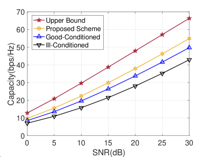
Figure 2: Capacity v.s. transmit SNR, $N_{t}=32$, $N_{r}=8$, $N_{\mathrm{cl}}=10$, $N_{\mathrm{ray}}=8$, physical and pattern channels.

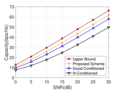
Figure 3: Capacity v.s. transmit SNR, $N_{t}=32$, $N_{r}=8$, $N_{\mathrm{cl}}=20$, $N_{\mathrm{ray}}=8$, physical and pattern channels.

We consider that $\alpha_{i,j}$ follows $\mathcal{C}\mathcal{N}\left(0,\sigma_{i}^{2}\right)$, where $\sigma_{i}^{2}$ represents the average power of the $i$-th cluster with $\sum_{i=1}^{N_{\mathrm{cl}}}\sigma_{i}^{2}=\gamma$. We introduce $\gamma$ as the normalization factor so that the power constraint of the channel matrix $\mathbb{E}\left\{\left\|\mathbf{H}\right\|_{\mathrm{F}}^{2}\right\}=N_{r}N_{t}$ can be held. $\theta_{i,l}$ is uniformly distributed with mean $\theta_{i}$ and a standard deviation $\xi$, and $\varphi_{i,l}$ is uniformly distributed with mean $\varphi_{i}$ and the same standard deviation $\xi$. In order to distinguish the physical channel quality, we define the good-conditioned channel whose $\left\{\sigma_{i}^{2}\right\}$ are the normal random variables to obtain a relatively small channel condition number, and the ill-conditioned channel with $\sigma_{1}^{2}:\sigma_{2}^{2}:\sigma_{3}^{2}:\sigma_{4}^{2}:\ldots:\sigma_{N_{\mathrm{cl}}}^{2}=100:50:50:1:\ldots:1$ so that the channel condition number will be large. All the results are obtained by averaging over 1000 Monte Carlo simulations. Unless otherwise stated, $N_{t}=32$, $N_{r}=8$, $\xi=3^{\circ}$, and the half-wavelength antenna spacing is held for all simulations. Both $\theta_{i}$ and $\varphi_{i}$ are uniformly distributed in the range of $\left[-\pi/2,\pi/2\right]$. We adopt the ideal channel $\mathbf{H}_{\mathrm{opt}}=\sqrt{N_{t}}\mathbf{I}_{N_{r}\times N_{t}}$ as the theoretical performance upper bound.

Fig. 2 compares the performance of the proposed pattern design scheme with the theoretical ideal channel, the good-conditioned channel and the ill-conditioned channel, when $N_{\mathrm{cl}}=10$. We can see that the proposed pattern design scheme can improve the capacity performance compared with the physical channel, which validates that the quality of the channel can be significantly improved by the pattern modification effect. Meanwhile, the gap between the proposed scheme and the theoretical upper bound reveals that the inability of phase adjustment prevents the further performance improvement of the PE-MIMO system.

Fig. 3 shows the analogous simulation results of Fig. 2 when $N_{\mathrm{cl}}=20$. Compared with Fig. 2, the additional subchannels provide more spatial DoFs so that the achievable capacity of the physical channel in good condition is improved. Moreover, the smaller gap between the performance of the proposed pattern design scheme and the theoretical upper bound reveals that the increasing scattering clusters provide additional DoFs which improves the pattern modification effect.

VI Conclusion

In this paper, we study a wireless communication system towards EIT that is able to configure the data transmission and electro-magnetic field distribution via the concept of PR-MIMO. Based on the matrix representation of PR-MIMO we propose, it is shown that the effect of radiation reconfigurability can be regarded as an additional gain on the corresponding propagation directions, and the capacity maximization pattern design problem is further formulated. We further decompose the optimal pattern design into the correlation modification process and the power allocation process, and propose an efficient design algorithm. More specifically, the channel correlation structure is optimized via the correlation modification matrix in the correlation modification process. Subsequently, based on the optimized subchannels, the transmission power is redistributed wisely in the power allocation process. Based on that, for the correlation modification process, we propose a sequential optimization framework with eigenvalue decomposition. For the power allocation process, a closed-form scheme is designed to improve the channel quality. Numerical results validate the superiority of PR-MIMO over traditional MIMO systems as well as the effectiveness of proposed algorithms. The future work will discuss the combination between PR-MIMO and constructive interference precoding [25].

References

- [1] L. Zheng and D. N. C. Tse, “Diversity and Multiplexing: A Fundamental Tradeoff in Multiple-Antenna Channels,” IEEE Transactions on Information Theory, vol. 49, no. 5, pp. 1073–1096, 2003.
- [2] Z. Zhang and L. Dai, “Continuous-Aperture MIMO for Electromagnetic Information Theory,” arXiv preprint arXiv:2111.08630, 2021.
- [3] S. Elgiddawy, H. A. Malhat, S. H. Zainud-Deen, A. A. Ibrahim, and H. Hamed, “Compact Reconfigurable Polarization Plasma Square Microstrip Patch MIMO Antenna for 5G Wireless Applications,” in 2021 38th National Radio Science Conference (NRSC), vol. 1, 2021, pp. 88–95.
- [4] P. Sanchez-Olivares and J. Masa-Campos, “Mechanically Reconfigurable Conformal Array Antenna Fed by Radial Waveguide Divider With Tuning Screws,” IEEE Transactions on Antennas and Propagation, vol. 65, no. 9, pp. 4886–4890, 2017.
- [5] B. A. Cetiner, E. Akay, E. Sengul, and E. Ayanoglu, “A MIMO System with Multifunctional Reconfigurable Antennas,” IEEE Antennas and Wireless Propagation Letters, vol. 5, pp. 463–466, 2006.
- [6] N. Ojaroudi Parchin, H. Jahanbakhsh Basherlou, Y. I. Al-Yasir, R. A. Abd-Alhameed, A. M. Abdulkhaleq, and J. M. Noras, “Recent Developments of Reconfigurable Antennas for Current And Future Wireless Communication Systems,” Electronics, vol. 8, no. 2, p. 128, 2019.
- [7] Y.-F. Cheng, X. Ding, B.-Z. Wang, and W. Shao, “An Azimuth-Pattern-Reconfigurable Antenna With Enhanced Gain and Front-to-Back Ratio,” IEEE Antennas and Wireless Propagation Letters, vol. 16, pp. 2303–2306, 2017.
- [8] M.-I. Lai, T.-Y. Wu, J.-C. Hsieh, C.-H. Wang, and S.-K. Jeng, “Compact Switched-Beam Antenna Employing a Four-Element Slot Antenna Array for Digital Home Applications,” IEEE Transactions on Antennas and Propagation, vol. 56, no. 9, pp. 2929–2936, 2008.
- [9] Y. Zhou, R. S. Adve, and S. V. Hum, “Design and Evaluation of Pattern Reconfigurable Antennas for MIMO Applications,” IEEE Transactions on Antennas and Propagation, vol. 62, no. 3, pp. 1084–1092, 2013.
- [10] A. Pal, A. Mehta, D. Mirshekar-Syahkal, and H. Nakano, “A Twelve-Beam Steering Low-Profile Patch Antenna With Shorting Vias for Vehicular Applications,” IEEE Transactions on Antennas and propagation, vol. 65, no. 8, pp. 3905–3912, 2017.
- [11] J.-S. Row and C.-W. Tsai, “Pattern Reconfigurable Antenna Array With Circular Polarization,” IEEE Transactions on Antennas and Propagation, vol. 64, no. 4, pp. 1525–1530, 2016.
- [12] M. Hasan, I. Bahceci, and B. A. Cetiner, “Downlink Multi-User MIMO Transmission for Radiation Pattern Reconfigurable Antenna Systems,” IEEE Transactions on Wireless Communications, vol. 17, no. 10, pp. 6448–6463, 2018.
- [13] A. C. Gurbuz, R. Mdrafi, and B. A. Cetiner, “Cognitive Radar Target Detection and Tracking With Multifunctional Reconfigurable Antennas,” IEEE Aerospace and Electronic Systems Magazine, vol. 35, no. 6, pp. 64–76, 2020.
- [14] E. Kaderli, İ. Bahçeci, K. M. Kaplan, and B. A. Cetiner, “On The Use of Reconfigurable Antenna Arrays for DoA Estimation of Correlated Signals,” in 2016 IEEE Radar Conference (RadarConf), 2016, pp. 1–5.
- [15] A. C. Gurbuz and B. Cetiner, “Multifunctional Reconfigurable Antennas for Cognitive Radars,” in 2018 IEEE Radar Conference (RadarConf18), 2018, pp. 1510–1515.
- [16] I. Bahceci, M. Hasan, T. M. Duman, and B. A. Cetiner, “Efficient Channel Estimation for Reconfigurable MIMO Antennas: Training Techniques and Performance Analysis,” IEEE Transactions on Wireless Communications, vol. 16, no. 1, pp. 565–580, 2016.
- [17] R. S. Sutton and A. G. Barto, Reinforcement Learning: An Introduction. MIT press, 2018.
- [18] N. Gulati and K. R. Dandekar, “Learning State Selection for Reconfigurable Antennas: A Multi-Armed Bandit Approach,” IEEE Transactions on Antennas and Propagation, vol. 62, no. 3, pp. 1027–1038, 2013.
- [19] T. Zhao, M. Li, and G. Ditzler, “Online Reconfigurable Antenna State Selection Based on Thompson Sampling,” in 2019 International Conference on Computing, Networking and Communications (ICNC), 2019, pp. 888–893.
- [20] T. Zhao, M. Li, and M. Poloczek, “Fast Reconfigurable Antenna State Selection with Hierarchical Thompson Sampling,” in ICC 2019-2019 IEEE International Conference on Communications (ICC), 2019, pp. 1–6.
- [21] T. Zhao, M. Li, and Y. Pan, “Online Learning Based Reconfigurable Antenna Mode Selection Exploiting Channel Correlation,” IEEE Transactions on Wireless Communications, 2021.
- [22] B. He and H. Jafarkhani, “Low-Complexity Reconfigurable MIMO for Millimeter Wave Communications,” IEEE Transactions on Communications, vol. 66, no. 11, pp. 5278–5291, 2018.
- [23] S. Burer, K. M. Anstreicher, and M. Dür, “The Difference Between 5 5 Doubly Nonnegative and Completely Positive Matrices,” Linear Algebra and its Applications, vol. 431, no. 9, pp. 1539–1552, 2009.
- [24] R. A. Horn and C. R. Johnson, Matrix Analysis. Cambridge university press, 2012.
- [25] A. Li, D. Spano, J. Krivochiza, S. Domouchtsidis, C. G. Tsinos, C. Masouros, S. Chatzinotas, Y. Li, B. Vucetic, and B. Ottersten, “A Tutorial on Interference Exploitation via Symbol-Level Precoding: Overview, State-of-the-Art and Future Directions,” IEEE Communications Surveys & Tutorials, vol. 22, no. 2, pp. 796–839, 2020.