ELLE: Efficient Lifelong Pre-training for Emerging Data

Abstract

Current pre-trained language models (PLM) are typically trained with static data, ignoring that in real-world scenarios, streaming data of various sources may continuously grow. This requires PLMs to integrate the information from all the sources in a lifelong manner. Although this goal could be achieved by exhaustive pre-training on all the existing data, such a process is known to be computationally expensive. To this end, we propose ELLE, aiming at efficient lifelong pre-training for emerging data. Specifically, ELLE consists of (1) function preserved model expansion, which flexibly expands an existing PLM’s width and depth to improve the efficiency of knowledge acquisition; and (2) pre-trained domain prompts, which disentangle the versatile knowledge learned during pre-training and stimulate the proper knowledge for downstream tasks. We experiment ELLE with streaming data from $5$ domains on BERT and GPT. The results show the superiority of ELLE over various lifelong learning baselines in both pre-training efficiency and downstream performances. The codes are publicly available at https://github.com/thunlp/ELLE.

1 Introduction

Pre-trained language models (PLM) have broken the glass ceiling for various natural language processing (NLP) tasks (Radford et al., 2018; Devlin et al., 2019; Han et al., 2021). However, most of the existing PLMs are typically trained with a static snapshot of the web information, ignoring that in real-world scenarios, streaming data from various sources may continuously grow, e.g., the gatherings of literary works (Zhu et al., 2015), news articles (Zellers et al., 2019) and science papers (Lo et al., 2020). In addition, the distribution of incoming data may also vary over time. This requires PLMs to continually integrate the information from all the sources to grasp the versatile structural and semantic knowledge comprehensively, so that PLMs could utilize the proper knowledge to boost the performance in various downstream tasks.

A simple yet effective way to integrate all the information is to pre-train PLMs on all the existing data exhaustively. However, such a process is computationally expensive (Schwartz et al., 2019), especially under the information explosion era when tremendous data is continually collected. This leaves us an important question: with limited computational resources, how can we efficiently adapt PLMs in a lifelong manner? We formulate it as the efficient lifelong pre-training problem. Similar to conventional lifelong learning, PLMs are expected to continually absorb knowledge from emerging data, and in the meantime, mitigate the catastrophic forgetting (McCloskey and Cohen, 20p) of previously learned knowledge.

In addition, efficient lifelong pre-training poses two new challenges: (1) efficient knowledge growth. When the overall data scale accumulates to a certain magnitude, packing more knowledge into a fixed-sized PLM becomes increasingly hard, which significantly impacts the efficiency of PLM’s knowledge growth. This is because larger PLMs show superior sample efficiency and training efficiency over their smaller counterparts (Kaplan et al., 2020; Li et al., 2020) due to overparameterization (Arora et al., 2018). That is, larger PLMs learn knowledge in a more efficient way. Therefore, timely model expansions are essential for efficient knowledge growth; (2) proper knowledge stimulation. During pre-training, various knowledge from all domains is packed into PLMs hastily. However, a certain downstream task may largely require the knowledge from a specific domain. Thus it is essential for PLMs to disentangle different kinds of knowledge and properly stimulate the needed knowledge for each task.

In this paper, we propose ELLE, targeting at Efficient LifeLong pre-training for Emerging data. Specifically, (1) to facilitate the efficiency of knowledge growth, we propose the function preserved model expansion to flexibly expand an existing PLM’s width and depth. In this way, we increase PLM’s model size and thus improve its training efficiency. Before being adapted to a new domain, the expanded PLM performs a function recovering warmup to regain the functionality of the original PLM; (2) for proper knowledge stimulation, we pre-implant domain prompts during pre-training to prime the PLM which kind of knowledge it is learning. Therefore, versatile knowledge from multiple sources can be disentangled. During downstream fine-tuning, we could further utilize these implanted prompts and manipulate the PLM to stimulate the proper knowledge for a specific task.

To demonstrate the effectiveness of ELLE, we simulate the scenario where streaming data from $5$ domains sequentially comes. We pre-train two typical PLMs (BERT and GPT) and expand their model sizes each time when the new data is available. We experiment when the number of parameters is sequentially grown from both $30$M to $125$M and $125$M to $355$M. The experimental results show the superiority of ELLE over multiple lifelong learning baselines in both pre-training efficiency and downstream task performances. In addition, we conduct sufficient experiments to verify the effectiveness of each component of ELLE. In general, we provide a promising research direction and hope this work could inspire more future attempts towards efficient lifelong pre-training.

2 Related Work

Lifelong Learning for PLMs.

Lifelong learning aims at incrementally acquiring new knowledge, and in the meantime, mitigating the catastrophic forgetting issue. Numerous efforts have been spent towards this goal, including (1) memory-based methods (Rebuffi et al., 2017; Rolnick et al., 2019), which perform experience replay with authentic data (de Masson d’Autume et al., 2019), automatically generated data (Sun et al., 2020), or previously computed gradients (Lopez-Paz and Ranzato, 2017) conserved in the memory, (2) consolidation-based methods (Kirkpatrick et al., 2017; Aljundi et al., 2018), which introduce additional regularization terms to consolidate the model parameters that are important to previous tasks, and (3) dynamic architecture methods (Rusu et al., 2016; Yoon et al., 2018), which fix trained network architectures in old tasks and dynamically grow branches for new tasks. Lifelong learning is also a hot topic for PLMs. Some target at domain adaptation through continual pre-training (Gururangan et al., 2020), parameter-efficient adapters (He et al., 2021) and sparse expert models (Gururangan et al., 2021). Others focus on the incremental acquisition of factual knowledge that changes over time (Dhingra et al., 2021; Jang et al., 2021). However, the existing works seldom consider our lifelong learning setting where streaming data from multiple sources is sequentially gathered. Recently, researchers have also conducted a series of empirical studies on the continual learning of PLMs (Wu et al., 2021; Jin et al., 2021).

Efficient Pre-training in NLP.

Many attempts have been made towards improving the efficiency of pre-training, such as designing novel pre-training tasks (Clark et al., 2020), model architectures (Zhang and He, 2020), optimization algorithms (You et al., 2020) and parallel architectures (Shoeybi et al., 2019; Shazeer et al., 2018). Until recently, researchers propose to “back distill” the knowledge from existing PLMs to accelerate large PLMs’ pre-training (Qin et al., 2021a). Another line of work proposes progressive training to dynamically expand an existing PLM’s size through parameter recycling (Gong et al., 2019; Gu et al., 2021; Chen et al., 2021). However, these methods typically focus on training PLMs on one static corpus, and thus cannot be directly applied to our lifelong pre-training setting.

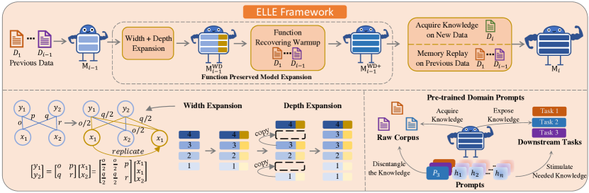
Figure 1: Illustration of ELLE when adapting an existing PLM $\mathcal{M}_{i-1}$ trained on previous data $\overline{\mathcal{D}}_{i-1}$ to a new corpus $\mathcal{D}_{i}$. We also visualize the mechanism of width / depth expansion and pre-trained domain prompts.

3 Methodology

3.1 Preliminaries

Background for PLM.

A PLM $\mathcal{M}$ generally consists of an embedding layer and $L$ Transformer (Vaswani et al., 2017) layers. Given an input $\mathbf{x}$ consisting of a series of tokens, i.e., $\mathbf{x}=\{w_{1},\dots,w_{|\mathbf{x}|}\}$, $\mathcal{M}$ first converts the input into embeddings $\{\mathbf{h}_{1}^{0},\dots,\mathbf{h}_{|\mathbf{x}|}^{0}\}$, which are sequentially processed by each Transformer layer into contextualized hidden representations $\mathbf{H}^{l}=\{\mathbf{h}_{1}^{l},\dots,\mathbf{h}_{|\mathbf{x}|}^{l}\}$, where $1\!\leq\!l\!\leq\!L$.

Task Definition.

Assume a stream of corpus $\overline{\mathcal{D}}_{N}$ from $N$ domains (e.g., news articles, web content and literary works) is sequentially gathered, i.e., $\overline{\mathcal{D}}_{N}=\{\mathcal{D}_{1},\dots,\mathcal{D}_{N}\}$, where $\mathcal{D}_{i}=\{\mathbf{x}_{i}^{j}\}_{j=1}^{|\mathcal{D}_{i}|}$. The whole training process can be partitioned into several stages. Initially, we have a PLM $\mathcal{M}_{1}$, which has been well trained on $\mathcal{D}_{1}$, and for the $i$-th stage ($i>1$), we obtain a new collection of data $\mathcal{D}_{i}$. Assume in this stage, we only have limited computational resources $\mathcal{R}_{i}$, our goal is to continually pre-train the existing PLM $\mathcal{M}_{i-1}$ to learn new knowledge on $\mathcal{D}_{i}$, and obtain a new PLM $\mathcal{M}_{i}$. Meanwhile, we expect the adapted PLM $\mathcal{M}_{i}$ should not forget the previously learned knowledge of $\overline{\mathcal{D}}_{i-1}$.

Overall Framework.

As illustrated in Figure 1, starting from $\mathcal{M}_{i-1}$, which is trained on previous data $\overline{\mathcal{D}}_{i-1}$, we first expand $\mathcal{M}_{i-1}$’s width and depth and construct an enlarged PLM $\mathcal{M}_{i-1}^{\text{WD}}$ to improve its training efficiency. Then we perform function recovering warmup and train $\mathcal{M}_{i-1}^{\text{WD}}$ to inherit the knowledge of $\mathcal{M}_{i-1}$ to obtain $\mathcal{M}_{i-1}^{\text{WD+}}$. The above procedures are dubbed as function preserved model expansion (§ 3.2). After that, we continually pre-train $\mathcal{M}_{i-1}^{\text{WD+}}$ to gain new knowledge on $\mathcal{D}_{i}$. To mitigate the catastrophic forgetting on the previously learned knowledge, we employ data-based memory replay on a subset of previously gathered data $\overline{\mathcal{D}}_{i-1}^{sub}=\{\mathcal{D}_{1}^{sub},\dots,\mathcal{D}_{i-1}^{sub}\}$ conserved in the memory, where $\mathcal{D}^{sub}_{k}=\{x_{k}^{1},\dots,x_{k}^{B}\}\in\mathcal{D}_{k}$ ($1\leq k\leq i-1$) and $B$ is the constrained memory size for each domain. To help PLMs disentangle the knowledge during pre-training and also stimulate the needed knowledge for each downstream task, we implant domain prompts into PLMs during the whole training process (§ 3.3).

3.2 Function Preserved Model Expansion

To accumulate knowledge more efficiently, each time when a new corpus $\mathcal{D}_{i}$ comes, we expand both $\mathcal{M}_{i-1}$’s width and depth to attain the superior sample efficiency and fast convergence brought by larger model capacity (Li et al., 2020).

Width Expansion.

For width expansion, we borrow the function preserving initialization (FPI) from Chen et al. (2021). For a brief introduction, FPI expands the matrices of all modules of a Transformer layer to arbitrary larger sizes and constructs an enlarged PLM $\mathcal{M}_{i-1}^{\text{W}}$. $\mathcal{M}_{i-1}^{\text{W}}$ is initialized using the corresponding matrices of the original $\mathcal{M}_{i-1}$ through parameter replication. For example, as visualized in Figure 1, the core principle of FPI is to divide the product of $o\times x_{1}$ into multiple partitions, e.g. $\frac{o}{2}\times x_{1}+\frac{o}{2}\times x_{1}$. Formally, FPI expands a matrix $\bm{W}\in\mathbb{R}^{h_{1}\times h_{2}}$ of $\mathcal{M}_{i-1}$ to an enlarged matrix $\bm{W}^{\prime}\in\mathbb{R}^{(h_{1}+\Delta_{h_{1}})\times h_{2}}$ of $\mathcal{M}_{i-1}^{\text{W}}$ as follows:

$$m(i) =\begin{cases}i&i\in[1,h_{1}]\\ U(\{1,\dots,h_{1}\})&i\in(h_{1},h_{1}+\Delta_{h_{1}}],\end{cases}$$ (1)

$$C_{i} =\sum_{i^{\prime}=1}^{h_{1}+\Delta_{h_{1}}}\mathbbm{I}({m(i^{\prime})=m(i)}),$$

$$\bm{W}^{\prime}_{(i,*)} =\frac{1}{C_{i}}\cdot\bm{W}_{(m(i),*)}+\mathbbm{I}(C_{i}>1)\cdot\bm{\delta}_{i},$$

where $U(\cdot)$ denotes a uniform sampling function, $m(\cdot)$ denotes the mapping function between two matrices, $\mathbbm{I}(\cdot)$ is an indicator function, $C_{i}$ counts how many partitions a specific neuron is splitted and $\bm{\delta}_{i}\in\mathbb{R}^{h_{2}}$ is a random gaussian noise. FPI ensures that both $\mathcal{M}_{i-1}^{\text{W}}$ and $\mathcal{M}_{i-1}$ have approximately the same functionality, i.e., both models have almost the same output given the same input. Besides function preservation, the initialized model could serve as a good starting point for further optimization. We refer readers to Chen et al. (2021) for more details about width expansion. Different from Chen et al. (2021), we additionally introduce random noises $\bm{\delta}_{i}$ into the newly copied parameters of $\bm{W}^{\prime}$ during initialization. These slight noises would break the symmetry after the replication and accelerate later pre-training.

Depth Expansion.

For depth expansion, previous works generally resort to stacking all the original PLM layers into $2\times$ layers through parameter replication (Gong et al., 2019). Such initialization is demonstrated to improve training efficiency.

However, the above layer stacking method restricts the number of layers of the enlarged PLM $\mathcal{M}_{i-1}^{\text{D}}$ to be integer multiples of that of the original PLM $\mathcal{M}_{i-1}$, which is not flexible for practical uses. To improve the expansion flexibility so that $\mathcal{M}_{i-1}$ could be expanded with arbitrary number of layers, we propose a novel layer insertion method to construct a new PLM $\mathcal{M}_{i-1}^{\text{D}}$ with $L+L^{\prime}$ layers, where $1\leq L^{\prime}\leq L$. Specifically, we randomly select $L^{\prime}$ layers from $\mathcal{M}_{i-1}$, copy each layer’s parameters and insert the replication layer right before / after the original layer. We found empirically that inserting the copied layer into other positions would cause a performance drop, and the reason is that it will violate the processing order of the original layer sequence and break the PLM’s original functionality. At each expansion stage when new data comes, since different layers have different functionalities, we always choose those layers that have not been copied before to help PLMs develop in an all-around way, instead of just developing a certain kind of functionality. Since both width expansion and depth expansion are compatible with each other, we simultaneously expand both of them to construct an enlarged model $\mathcal{M}_{i-1}^{\text{WD}}$, which inherits $\mathcal{M}_{i-1}$’s knowledge contained in the parameters.

Function Recovering Warmup.

Since the above model expansion cannot ensure exact function preservation and inevitably results in functionality loss and performance drops, we pre-train the initialized PLM $\mathcal{M}_{i-1}^{\text{WD}}$ on the previous corpora $\overline{\mathcal{D}}_{i-1}^{sub}$ conserved in the memory to recover the language abilities lost during model expansion, which is dubbed as function recovering warmup (FRW). After the warmup, we obtain $\mathcal{M}_{i-1}^{\text{WD+}}$, which successfully inherits the knowledge from $\mathcal{M}_{i-1}$ and is also well-prepared for the next training stage.

3.3 Pre-trained Domain Prompt

Instead of training a separate model for each domain, we expect a single compact PLM to integrate the knowledge from all the sources. When confronted with a downstream task from a specific domain, the PLM needs to expose the proper knowledge learned during pre-training. To facilitate both knowledge acquisition during pre-training and knowledge exposure during fine-tuning, we resort to prompts as domain indicators and condition the PLM’s behavior on these prompts. Soft prompts have been demonstrated as excellent task indicators (Qin et al., 2021b) and have non-trivial transferability among tasks (Su et al., 2021).

Specifically, during pre-training, to disentangle the knowledge from different sources, we implant a soft prompt token into the input to prime the PLM which kind of knowledge it is learning. The prompt of domain $i$ is a tunable vector $\mathbf{p}_{i}$. We prepend $\mathbf{p}_{i}$ before the original token embeddings $\mathbf{H}^{0}=\{\mathbf{h}^{0}_{1},\dots,\mathbf{h}^{0}_{|\mathbf{x}|}\}$ for an input $\mathbf{x}\in\mathcal{D}_{i}$, resulting in the modified input $\mathbf{H}^{0*}=\{\mathbf{p}_{i};\mathbf{h}^{0}_{1},\dots,\mathbf{h}^{0}_{|\mathbf{x}|}\}$, which is then processed by all the Transformer layers. Each $\mathbf{p}_{i}$ is optimized together with other parameters of the PLM during pre-training. During fine-tuning, when applying the PLM on a similar domain of data seen before, we could leverage the trained domain prompt and prepend it before the input of downstream data. In this way, we manually manipulate the PLM to stimulate the most relevant knowledge learned during pre-training.

4 Experiments

Domain	WB		Ns		Rev		Bio		CS
Metrics	AP	AP+	AP	AP+	AP	AP+	AP	AP+	AP	AP+
Growing from $\text{BERT}_{\text{L6\_D384}}$ to $\text{BERT}_{\text{L12\_D768}}$
Naive (Lower Bound)	$7.96$	-	$8.03$	$5.54$	$13.52$	$21.42$	$13.86$	$17.67$	$9.93$	$9.81$
EWC	$7.96$	-	$8.09$	$5.65$	$13.40$	$20.98$	$13.92$	$17.75$	$9.94$	$9.82$
MAS	$7.96$	-	$8.08$	$5.65$	$13.44$	$21.17$	$13.87$	$17.67$	$9.91$	$9.75$
A-GEM	$7.96$	-	$8.82$	$6.72$	$13.31$	$20.06$	$14.73$	$18.89$	$10.56$	$10.58$
ER	$7.96$	-	$6.85$	$1.59$	$6.99$	$4.09$	$6.66$	$3.62$	$6.39$	$3.16$
Logit-KD	$7.96$	-	$7.60$	$0.99$	$7.19$	$1.95$	$7.08$	$2.02$	$6.92$	$1.92$
PNN	$7.96$	-	$6.52$	$0.00$	$5.29$	0.00	$4.84$	0.00	$4.76$	0.00
ELLE (ours)	7.92	-	5.62	-0.20	4.81	$0.64$	4.41	$0.64$	4.06	$0.44$
Growing from $\text{BERT}_{\text{L12\_D768}}$ to $\text{BERT}_{\text{L24\_D1024}}$
ER	$4.54$	-	$4.33$	$1.31$	$4.02$	$1.46$	$3.73$	$1.15$	$3.82$	$1.28$
ELLE (ours)	4.52	-	3.89	0.47	3.61	0.75	3.66	0.97	3.29	0.54
Growing from $\text{GPT}_{\text{L6\_D384}}$ to $\text{GPT}_{\text{L12\_D768}}$
Naive (Lower Bound)	$46.54$	-	$52.91$	$37.96$	$81.28$	$177.22$	$94.44$	$160.51$	$60.64$	$80.48$
MAS	$46.54$	-	$53.12$	$38.44$	$81.23$	$177.20$	$93.21$	$157.93$	$60.62$	$80.28$
ER	$46.54$	-	$44.49$	$12.42$	$35.46$	$21.78$	$33.24$	$23.38$	$31.94$	$19.83$
Logit-KD	$46.54$	-	$48.93$	$5.41$	$37.60$	$9.97$	$34.60$	$11.74$	$33.67$	$11.19$
PNN	$46.54$	-	$39.90$	0.00	$26.84$	0.00	22.19	0.00	$21.43$	0.00
ELLE (ours)	46.50	-	36.84	$2.25$	25.60	$4.38$	$22.29$	$5.88$	20.49	$4.31$

Table 1: Average perplexity (AP) and average increased perplexity ($\text{AP}^{+}$) of PLMs trained by different lifelong learning methods with the same train wall time. PLMs are trained with streaming data from WB, Ns, Rev, Bio and CS domain sequentially. We evaluate the performance each time when PLMs finish training on one domain.

4.1 Experimental Setting

Data Streams.

We simulate the scenario where streaming data from $5$ domains is gathered sequentially, i.e., the concatenation of Wikipedia and BookCorpus (WB) (Zhu et al., 2015), News Articles (Ns) (Zellers et al., 2019), Amazon Reviews (Rev) (He and McAuley, 2016), Biomedical Papers (Bio) (Lo et al., 2020) and Computer Science Papers (CS) (Lo et al., 2020). For each corpus $\mathcal{D}_{i}$, we roughly sample $3,400$M tokens, and the quantity for each $\mathcal{D}_{i}$ ($1\leq i\leq 5$) is comparable to the pre-training data of BERT (Devlin et al., 2019). In addition, considering that in practice, the expense of storage is far cheaper than the computational resources for pre-training, we maintain a relatively large memory compared with conventional lifelong learning settings by randomly sampling $200$M tokens ($\mathcal{D}_{i}^{sub}$) for each corpus $\mathcal{D}_{i}$.

Evaluated Models.

We mainly follow the model architectures of BERT and GPT (Radford et al., 2018). We use byte-level BPE vocabulary to ensure there are few unknown tokens in each corpus. We experiment with the initial PLM $\mathcal{M}_{1}$ of $6$ layers and hidden size of $384$ (around $30$M parameters, denoted as $\text{BERT}_{\text{L6\_D384}}$ / $\text{GPT}_{\text{L6\_D384}}$), and linearly enlarge the PLM’s number of parameters for $4$ times, to the final PLM $\mathcal{M}_{5}$ of $12$ layers and hidden size of $768$ (around $125$M parameters, denoted as $\text{BERT}_{\text{L12\_D768}}$ / $\text{GPT}_{\text{L12\_D768}}$). We also experiment on a larger model size, i.e., growing the PLM from $\text{BERT}_{\text{L12\_D768}}$ ($125$M) to $\text{BERT}_{\text{L24\_D1024}}$ ($355$M). Details of each $\mathcal{M}_{i}$’s architecture are listed in appendix B. We also discuss the effect of expanded model size at each stage in appendix A.

Training Details.

We train our model for $62,500$ steps for the first corpus. For the following domain $i$ ($i>1$), after the model expansion, we perform function recovering warmup for $5,000$ steps, then train the resulting PLM for $20,000$ steps on the new data together with memory replay. Following Chaudhry et al. (2019b), we jointly train PLMs on a mixture samples from both $\mathcal{D}_{i}$ and $\overline{\mathcal{D}}_{i-1}^{sub}$ in each batch, and the sampling ratio of $\mathcal{D}_{i}$ and $\overline{\mathcal{D}}_{i-1}^{sub}$ is set to $9:1$ in every batch. Adam (Kingma and Ba, 2015) is chosen as the optimizer. All the experiments are conducted under the same environment of $8$ V100 GPUs with a batch size of $2,048$. More training details of pre-training are left in appendix B. We also experiment with fewer computational budgets and memory budgets in appendix G, and find that within a reasonable range, both of the two factors would not significantly influence the performance of ELLE.

Evaluation Metrics.

We deem one algorithm to be more efficient if it could achieve the same performance as other methods utilizing fewer computations. For PLM, this is equivalent to achieving better performance using the same computations since pre-training with more computations almost always results in better performance (Clark et al., 2020). We evaluate the PLM’s performance during both pre-training and downstream fine-tuning.

Specifically, for pre-training, we propose two metrics to evaluate how PLMs perform on the learned domains following Chaudhry et al. (2019a): (1) average perplexity (AP) and (2) average increased perplexity ($\text{AP}^{+}$). We record the train wall time (Li et al., 2020) during pre-training. For a model checkpoint at time step $T$ when learning the $j$-th domain, we measure the checkpoint’s perplexity $\text{PPL}_{T,i}$ on the validation set of each domain $i$. Let $\text{PPL}_{i,i}^{f}$ be the perplexity on the $i$-th domain when the PLM finishes training on the $i$-th domain, the above metrics are calculated as follows:

AP $$=\exp{\big{(}\frac{1}{j}\sum\limits_{i=1}^{j}\log\text{PPL}_{T,i}\big{)}},$$ (2)

$$\text{AP}^{+} =\frac{1}{j-1}\sum\limits_{i=1}^{j-1}(\text{PPL}_{T,i}-\text{PPL}_{i,i}^{f}),$$

where AP measures the average performance on all the seen data $\{\mathcal{D}_{1},\ldots,\mathcal{D}_{j}\}$. Lower AP indicates the PLM generally learns more knowledge from existing domains; $\text{AP}^{+}$ measures the influence of current data $\mathcal{D}_{j}$ on previous data $\overline{\mathcal{D}}_{j-1}$. Lower $\text{AP}^{+}$ means PLMs forget less knowledge learned before.

To evaluate PLMs’ performance in downstream tasks, for each domain, we select a representative task that is relatively stable, i.e., MNLI (Williams et al., 2018), HyperPartisan (Kiesel et al., 2019), Helpfullness (McAuley et al., 2015), ChemProt (Kringelum et al., 2016) and ACL-ARC (Jurgens et al., 2018) for WB, Ns, Rev, Bio and CS, respectively. Training details for fine-tuning are left in appendix C.

Figure 2: Average perplexity (AP) of different lifelong learning methods with $\text{BERT}_{\text{L6\_D384}}$ as the initial PLM. The trend curves for $\text{AP}^{+}$ and other PLMs are left in appendix D.

Baselines.

Keeping most of the experimental settings the same, we choose the following baselines for comparison: (1) Naive, which is a naive extension of Gururangan et al. (2020) to continually adapt PLMs for each domain and can be seen as the lower bound; (2) EWC (Schwarz et al., 2018), which adopts elastic weight consolidation to add $L_{2}$ regularization on parameter changes; (3) MAS (Aljundi et al., 2018), which estimates parameter importance via the gradients of the model outputs; (4) ER (Chaudhry et al., 2019b), which alleviates forgetting by jointly training models on a mixture samples from new data $\mathcal{D}_{i}$ and the memory $\overline{\mathcal{D}}_{i-1}^{sub}$. ELLE is based on ER and additionally introduces the model expansion and pre-trained domain prompts. For ER, we set the sampling ratio of $\mathcal{D}_{i}$ and $\overline{\mathcal{D}}_{i-1}^{sub}$ to be $9:1$ in every batch same as ELLE; (5) A-GEM (Chaudhry et al., 2019a), which constrains the new parameter gradients to make sure that optimization directions do not conflict with gradients on old domains; (6) Logit-KD, which prevents forgetting by distilling knowledge from the previous model $\mathcal{M}_{i-1}$ using the old data in the memory; (7) PNN (Rusu et al., 2016), which fixes the old PLM $\mathcal{M}_{i-1}$ to completely avoid knowledge forgetting and grows new branches for learning new knowledge. For a fair comparison, we control the total train wall time of ELLE and all the baselines to be the same at each training stage, so that each method consumes the same computational costs.

Domain	WB	Ns	Rev	Bio	CS	AVG
Growing from $\text{BERT}_{\text{L6\_D384}}$ to $\text{BERT}_{\text{L12\_D768}}$
Naive	$77.2$	$72.8$	$60.6$	$77.1$	$64.8$	$70.5$
EWC	$77.4$	$72.8$	$61.6$	$77.5$	$59.6$	$69.8$
MAS	$77.1$	$73.7$	$60.7$	$77.5$	$68.2$	$71.5$
A-GEM	$76.6$	$71.4$	$61.5$	$76.9$	$67.5$	$70.8$
ER	$77.6$	$72.2$	$61.9$	$78.3$	$63.5$	$70.7$
Logit-KD	$77.2$	$69.5$	$63.9$	$76.8$	$58.9$	$69.2$
PNN	$76.0$	$76.3$	$68.0$	$79.5$	$65.2$	$73.0$
ELLE	83.2	81.8	68.5	82.9	72.7	77.8
Growing from $\text{BERT}_{\text{L12\_D768}}$ to $\text{BERT}_{\text{L24\_D1024}}$
ER	$84.7$	$83.3$	$68.0$	$82.7$	$71.4$	$78.0$
ELLE	86.3	90.4	70.5	84.2	73.8	81.0

Table 2: Final downstream performance (F1) of BERT on each domain after finishing pre-training on all domains. Experiments of Ns domain are repeated for 10 times with different seeds and others are repeated for 5 times. More detailed results at different pre-training stages are illustrated in appendix C.

4.2 Main Results

Table 1 summarizes the pre-training performance each time when the PLM finishes training on a specific domain. Figure 2 depicts the trend of AP for BERT w.r.t. train wall time, other trend curves are illustrated in appendix D. We also report the final downstream performance for discriminative PLMs (BERT) on each domain after finishing the whole pre-training in Table 2. The intermediate downstream performance each time when the PLM finishes training on one domain is left in appendix C.

Domain					WB		Ns		Rev		Bio		CS
WE	DE	FRW	$\delta_{N}$	PT	AP	AP+	AP	AP+	AP	AP+	AP	AP+	AP	AP+
					$7.96$	-	$6.85$	$1.59$	$6.99$	$4.09$	$6.66$	$3.62$	$6.39$	$3.16$
✓		✓			$7.96$	-	$6.23$	$0.78$	$5.34$	$1.42$	$4.98$	$1.20$	$4.48$	$0.89$
	✓	✓			$7.96$	-	$5.81$	$0.03$	$5.49$	$1.43$	$5.16$	$1.32$	$4.79$	$0.94$
✓	✓	✓			$7.96$	-	$5.78$	$0.02$	$4.91$	$0.76$	$4.49$	$0.73$	$4.13$	$0.52$
✓	✓				$7.96$	-	$5.79$	$0.09$	$5.09$	$1.13$	$4.58$	$0.88$	$4.22$	$0.65$
✓	✓	✓	✓		$7.96$	-	$5.69$	$-0.13$	$4.85$	$0.67$	$4.45$	$0.69$	$4.09$	$0.47$
✓	✓	✓	✓	✓	7.92	-	5.62	-0.20	4.81	0.64	4.41	0.64	4.06	0.44

Table 3: AP and $\text{AP}^{+}$ of different combinations of strategies when growing $\text{BERT}_{\text{L6\_D384}}$ to $\text{BERT}_{\text{L12\_D768}}$.

Superiority of ELLE.

(1) From the results in Table 1, we observe that, compared with all the baselines, ELLE achieves the lowest AP and satisfying $\text{AP}^{+}$ after finishing training on each domain. This demonstrates that, given limited computational resources, ELLE could acquire more knowledge and in the meantime, mitigate the knowledge forgetting problem. (2) We also observe from Figure 2 that the AP of ELLE descends the fastest, showing the superior training efficiency of ELLE over all baselines. (3) Besides, ELLE performs the best on all downstream tasks, indicating that the knowledge learned during pre-training could be properly stimulated and leveraged for each downstream task. (4) The superiority of ELLE is consistently observed on the larger model size, i.e., $\text{BERT}_{\text{L24\_D1024}}$ and other model architectures, i.e., $\text{GPT}_{\text{L12\_D768}}$. This shows that ELLE is agnostic to both the model size and the specific PLM model architecture chosen. We expect future work to apply ELLE to other PLM architectures and extremely large PLMs.

Comparisons with Baselines.

(1) First of all, consolidation-based methods (EWC and MAS) perform almost comparable with the naive baseline in either pre-training or downstream tasks. This means that parameter regularization may not be beneficial for PLMs’ knowledge acquisition. (2) Among memory-based methods, gradient-based replay (A-GEM) exhibits poorer performance in pre-training, on the contrary, data-based replay (ER and Logit-KD) achieve lower AP and $\text{AP}^{+}$ than the naive baseline, demonstrating that replaying real data points could more efficiently mitigate the knowledge forgetting problem. Meanwhile, all of the memory-based methods perform comparable or worse than the naive baseline in downstream performance. (3) PNN achieves significantly lower AP than non-progressive baselines, and is immune to knowledge forgetting ($\text{AP}^{+}\!\!=\!0$). It also performs better on the downstream tasks than other baselines. This indicates that enlarging the network is an effective way for lifelong pre-training and also benefits downstream tasks.

5 Analysis

In this section, we conduct analyses to investigate the effect of ELLE’s components. We follow the setting in § 4 by choosing $\text{BERT}_{\text{L6\_D384}}$ as the initial model and continually growing it to $\text{BERT}_{\text{L12\_D768}}$. Specifically, we investigate the effect of (1) width expansion (WE), (2) depth expansion (DE), (3) function recovering warmup (FRW), (4) the random noises added into the newly constructed parameters during model expansion ($\delta_{N}$) and (5) the pre-trained domain prompts (PT). We test ELLE under different combinations of the above components and compare the results. The experimental results of pre-training and downstream tasks are summarized in Table 3 and Table 4, respectively. Detailed trend curves for AP and $\text{AP}^{+}$ are illustrated in appendix D.

Effect of Width / Depth Expansion.

First, we compare the differences of conducting only width expansion (WE+FRW), only depth expansion (DE+FRW) and expansion on both width and depth (WE+DE+FRW) before function preserving warmup. For a fair comparison, we keep the total number of $\mathcal{M}_{i}$’s increased parameters for the above three strategies almost the same at each stage $i$. The specific model architectures are listed in appendix F. The results show that: (1) compared with the non-expanding baseline, all these three strategies achieve better pre-training and downstream performance, showing that with the growth of model size, the sample efficiency and training efficiency are extensively increased. Therefore, PLMs could gain more knowledge with limited computational resources and perform better in downstream tasks; (2) compared with expanding only width or depth, expanding both of them is more efficient and can also achieve better downstream performance on almost all domains, except the Ns domain. This is also aligned with previous findings that PLM’s growth favors compound scaling (Gu et al., 2021). We also conclude from the trend curves in appendix D that only expanding depth will make the training process unstable.

WE	DE	FRW	$\delta_{N}$	PT	WB	Ns	Rev	Bio	CS	AVG
					$77.6$	$72.2$	$61.9$	$78.3$	$63.5$	$70.7$
✓		✓			$81.9$	$77.5$	$64.9$	$80.3$	$70.7$	$75.1$
	✓	✓			$82.4$	$79.9$	$66.2$	$80.4$	$71.0$	$75.9$
✓	✓	✓			$83.4$	$74.7$	$67.4$	$82.4$	$72.2$	$76.0$
✓	✓				$82.6$	$75.7$	$67.4$	$82.3$	$71.4$	$75.9$
✓	✓	✓	✓		83.5	$77.1$	$66.9$	83.3	$71.3$	$76.4$
✓	✓	✓	✓	✓	$83.2$	81.8	68.5	$82.9$	72.7	77.8

Table 4: $\text{BERT}_{\text{L12\_D768}}$’s downstream performance (F1) on each domain after being continually pre-trained on all domains with different combinations of strategies.

Effect of Function Recovering Warmup.

We compare the performance of the model expansion w/ and w/o FRW, i.e., WE+DE and WE+DE+FRW. For a fair comparison, we keep the total train wall time for either strategy the same, in other words, for WE+DE, PLMs can be trained for more steps on the new domain due to the removal of FRW. However, the results show that WE+DE achieves worse AP and $\text{AP}^{+}$, indicating that without FRW, PLM would learn new knowledge slower and also forget more previous knowledge. The trend curve in appendix D also shows that AP and $\text{AP}^{+}$ decrease faster with FRW. This demonstrates the necessity of the warmup after model expansion, i.e., PLMs could better recover the knowledge lost during model expansion and also get prepared for learning new knowledge. Meanwhile, WE+DE+FRW performs slightly better than WE+DE in most of the downstream tasks, except the Ns domain.

Effect of Random Noises.

Different from the original FPI (Chen et al., 2021), ELLE additionally adds random noises into the newly copied parameters after expanding the width of PLMs as mentioned in § 3.2. By comparing the model performance w/ and w/o this trick, i.e., WE+DE+FRW and WE+DE+FRW+$\delta_{N}$, we can see that the added noises significantly speed up pre-training and also conduce to improving PLM’s overall downstream performance. This validates our hypothesis that random noises are useful for breaking the symmetry of the copied parameters, thus providing a better initialization that further optimization favors.

Effect of Pre-trained Domain Prompts.

To investigate the effect of pre-trained domain prompts, we first compare the performance w/ and w/o them, i.e., WE+DE+FRW+$\delta_{N}$ and WE+DE+FRW+$\delta_{N}$+PT. From the results we can conclude that when aided with domain prompts, PLMs achieve lower AP and $\text{AP}^{+}$ during pre-training, showing that domain prompts could accelerate pre-training and alleviate catastrophic forgetting by disentangling the knowledge from different sources. Furthermore, domain prompts generally improve downstream performance by stimulating the proper knowledge needed for each task.

Domain	WB	Ns	Rev	Bio	CS	AVG
ELLE $-$ $\text{PT}_{\text{fine-tune}}$	$82.9$	79.9	$67.0$	$82.1$	$67.7$	$75.9$
ELLE $+$ $\lnot\text{PT}_{\text{fine-tune}}$	$83.1$	$80.6$	$68.1$	$81.7$	$70.8$	$76.9$
ELLE	83.2	81.8	68.5	82.9	72.7	77.8

Table 5: $\text{BERT}_{\text{L12\_D768}}$’s downstream performance (F1) on each domain when no prompt / a wrong prompt is prepended in the input.

Figure 3: The visualization of the attention patterns of different attention heads in $\mathcal{M}_{1}$ ($\text{BERT}_{\text{L6\_D384}}$), $\mathcal{M}_{2}$ ($\text{BERT}_{\text{L8\_D512}}$), $\mathcal{M}_{3}$ ($\text{BERT}_{\text{L10\_D640}}$), $\mathcal{M}_{4}$ ($\text{BERT}_{\text{L11\_D708}}$) and $\mathcal{M}_{5}$ ($\text{BERT}_{\text{L12\_D768}}$) after finishing training on the new corpus $\mathcal{D}_{i}$. Note that in this figure, all the attention heads of a PLM $\mathcal{M}_{i}$ are expanded from all its ancestors $\{\mathcal{M}_{1},\dots,\mathcal{M}_{i-1}\}$ in the same column. We observe similar attention patterns between the descendant PLM and the ancestor PLM, demonstrating the descendant PLM successfully preserves the functionality of its ancestors.

To rigorously investigate how domain prompts stimulate the knowledge during fine-tuning, for a PLM pre-implanted with prompts during pre-training, we test its downstream performance when (1) no prompt is prepended in the input (i.e., ELLE- $\text{PT}_{\text{fine-tune}}$) during fine-tuning and (2) a prompt from a random wrong domain is prepended in the input (i.e., ELLE + $\lnot\text{PT}_{\text{fine-tune}}$). The results in Table 5 show that both of the above strategies have lower downstream performance than prepending the right prompt (ELLE). We hypothesize the reasons are two-fold: (1) firstly, for ELLE- $\text{PT}_{\text{fine-tune}}$, there exists a great gap between the formats of input during pre-training and fine-tuning, and such a gap would hinder the successful knowledge transfer; (2) secondly, for ELLE + $\lnot\text{PT}_{\text{fine-tune}}$, although the above gap disappears, the PLM is primed with a wrong domain prompt, and thus cannot properly stimulate the knowledge that is most relevant to the downstream task. Although manually deciding the most relevant domain prompt for a specific downstream task is relatively easy and fast, such a process can also be automated by training a domain discriminator, which is left as future work.

Attention Pattern Visualization of a Stream of PLMs.

Through the function preserved model expansion, PLMs inherit the knowledge of their “ancestors” contained in the parameters. Intuitively, the descendant PLM (the expanded larger PLM) should have similar functionalities to the ancestor PLM (the original PLM before model expansion). We thus investigate such functionality similarity through the lens of attention patterns of each attention head in the Transformer layer.

Specifically, we visualize the attention patterns of a stream of PLMs ($\{\mathcal{M}_{1},\ldots,\mathcal{M}_{5}\}$) trained by ELLE when growing from $\text{BERT}_{\text{L6\_D384}}$ to $\text{BERT}_{\text{L12\_D768}}$. We checkpoint each PLM $\mathcal{M}_{i}$ when it finishes training on the emerging data $\mathcal{D}_{i}$. We input the same data into these checkpoints to derive the attention patterns. The results are illustrated in Figure 3, from which we observe that the attention patterns of a head in a descendant PLM are surprisingly similar to those of its “ancestors”, even if the descendant PLM is further trained on the new data and enlarged many times. This indicates that the expanded PLM by ELLE successfully inherits the knowledge from its “ancestor”, and thus exhibits similar functionality to some extent.

6 Conclusion

In this paper, we present the efficient lifelong pre-training problem, which requires PLMs to continually integrate the information from emerging data efficiently. To achieve our goal, we propose ELLE and progressively expand PLMs to acquire knowledge efficiently and mitigate the knowledge forgetting. We also pre-implant domain prompts during pre-training and use them to stimulate the needed knowledge for downstream tasks. The experimental results show the superiority of ELLE over various lifelong learning baselines in both pre-training efficiency and downstream performances.

Appendices

Appendix A Additional Analysis on Function Preserved Model Expansion

In addition to the analyses of function preserved model expansion conducted in our main paper, in this section, we further analyze the effect of (1) the expanded model size at each training stage and (2) the choice of copied layer during depth expansion. We experiment on the combination of WE+DE+FRW as mentioned in § 5 and choose $\text{BERT}_{\text{L6\_D384}}$ as the initial PLM $\mathcal{M}_{1}$. Other settings are kept the same as § 5.

Domain	WB		News		Review
Metrics	AP	$\text{AP}^{+}$	AP	$\text{AP}^{+}$	AP	$\text{AP}^{+}$
Expand $0$ layers and heads per domain	13.09	-	$8.99$	$-0.49$	$8.24$	$2.80$
Expand $2$ layers and heads per domain	13.09	-	8.28	-1.44	7.25	1.11
Expand $4$ layers and heads per domain	13.09	-	$8.62$	$-0.95$	$7.53$	$1.30$
Expand $6$ layers and heads per domain	13.09	-	$9.08$	$-0.24$	$7.92$	$1.49$

Table 6: AP and $\text{AP}^{+}$ of PLMs trained with ELLE that expands $0$, $2$, $4$ and $6$ layers and heads during model expansion, respectively. AP and $\text{AP}^{+}$ are evaluated when each PLM finishes training on each domain.

Effect of Expanded Model Size.

In our main experiments, we assume that the data size of each emerging corpus is the same and linearly enlarge the model size when conducting model expansion. In this section, we explore the effect of expanded model size given limited computational resources. We conduct experiments on a stream of data from $3$ domains, i.e., WB, Ns and Rev domain. We start from the initial PLM $\text{BERT}_{\text{L6\_D384}}$ and continually adapt it to new corpora. Under the same training environment, we control the computational costs (train wall time) of each domain to be $7200$ seconds. We compare the performances when the PLM expands $0$, $2$, $4$, and $6$ layers and heads for each domain, respectively. Note the PLMs expanded with a larger size would be trained with fewer steps to control the train wall time.

The results are shown in Table 6, from which we can conclude that the best performance is obtained when the model expands $2$ layers and heads at each expansion stage, and expanding more or fewer parameters leads to a performance drop. The reasons are two-fold: (1) firstly, as mentioned before, expanding the model size improves the sample efficiency (Kaplan et al., 2020; Li et al., 2020), which is beneficial for PLMs’ knowledge acquisition; (2) secondly, when increasing the expanded model size, the benefits from inheriting the knowledge of a small PLM would become less and less evident. To sum up, expanding with an intermediate size strikes the best trade-off between the above two reasons, and there may exist an optimal expanded size when performing model expansion.

Intuitively, the optimal expanded model size may be influenced by many factors, e.g., the computational budgets, the amount of emerging data, the PLM’s model architecture, etc. And systematically analyzing the effects of all these factors is beyond the scope of this paper, thus we expect future works to design algorithms to accurately estimate the optimal expanded size for model expansion.

Choice of Copied Layer.

As mentioned in § 3.2, each time when we conduct width expansion, we choose those layers that have not been copied before. To demonstrate the benefit of this trick, we compare three expansion strategies: (1) always replicating those layers that have not been copied before (WE+DE+FRW); (2) always replicating the first layer (WE+$\text{DE}_{\text{first}}$+FRW) and (3) always replicating the last layer (WE+$\text{DE}_{\text{last}}$+FRW).

The results in Figure 4 show that AP and $\text{AP}^{+}$ descend the fastest when we always replicate those layers that have not been copied before (i.e., WE+DE+FRW). This demonstrates that, since different layers have different functionalities, choosing those layers that have not been expanded before would help PLMs develop in an all-around way, instead of just developing a certain kind of functionality. Furthermore, we find empirically that when pre-training PLMs continually on multiple domains, if we always choose those layers that have not been expanded before at each depth expansion stage, then the final performance is not sensitive to choosing which layers to expand first.

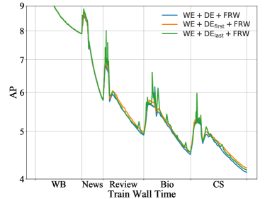
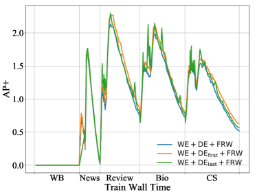
Figure 4: AP and $\text{AP}^{+}$ of PLMs trained by ELLE using different depth expansion strategies: WE+DE+FRW, WE+$\text{DE}_{\text{first}}$+FRW and WE+$\text{DE}_{\text{last}}$+FRW w.r.t train wall time.

Model	$n_{\text{params}}$	$n_{\text{layers}}$	$d_{\text{model}}$	$n_{\text{heads}}$	$d_{\text{FFN}}$	lr	SF	STF	RW	TWT(s)
Growing from $\text{BERT}_{\text{L6\_D384}}$ to $\text{BERT}_{\text{L12\_D768}}$
$\mathcal{M}_{1}$	$30.3$M	$6$	$384$	$6$	$1536$	$5.0\times 10^{-4}$	-	$62.5$k	$8\%$	$6.0\times 10^{4}$
$\mathcal{M}_{2}$	$51.5$M	$8$	$512$	$8$	$2048$	$5.0\times 10^{-4}$	$5$k	$20$k	$8\%$	$2.4\times 10^{4}$
$\mathcal{M}_{3}$	$82.2$M	$10$	$640$	$10$	$2560$	$5.0\times 10^{-4}$	$5$k	$20$k	$8\%$	$5.0\times 10^{4}$
$\mathcal{M}_{4}$	$102$M	$11$	$704$	$11$	$2816$	$5.0\times 10^{-4}$	$5$k	$20$k	$8\%$	$5.8\times 10^{4}$
$\mathcal{M}_{5}$	$125$M	$12$	$768$	$12$	$3072$	$5.0\times 10^{-4}$	$5$k	$20$k	$8\%$	$6.8\times 10^{4}$
Growing from $\text{BERT}_{\text{L12\_D768}}$ to $\text{BERT}_{\text{L24\_D1024}}$
$\mathcal{M}_{1}$	$125$M	$12$	$768$	$12$	$3072$	$5.0\times 10^{-4}$	-	$62.5$k	$8\%$	$1.9\times 10^{5}$
$\mathcal{M}_{2}$	$216$M	$15$	$960$	$15$	$3840$	$2.5\times 10^{-4}$	$1$k	$20$k	$20\%$	$6.5\times 10^{4}$
$\mathcal{M}_{3}$	$280$M	$18$	$1024$	$16$	$4096$	$2.5\times 10^{-4}$	$1$k	$20$k	$20\%$	$1.4\times 10^{5}$
$\mathcal{M}_{4}$	$318$M	$21$	$1024$	$16$	$4096$	$2.5\times 10^{-4}$	$1$k	$20$k	$20\%$	$1.7\times 10^{5}$
$\mathcal{M}_{5}$	$355$M	$24$	$1024$	$16$	$4096$	$2.5\times 10^{-4}$	$1$k	$20$k	$20\%$	$2.2\times 10^{5}$
Growing from $\text{GPT}_{\text{L6\_D384}}$ to $\text{GPT}_{\text{L12\_D768}}$
$\mathcal{M}_{1}$	$29.9$M	$6$	$384$	$6$	$1536$	$5.0\times 10^{-4}$	-	$62.5$k	$16\%$	$6.7\times 10^{4}$
$\mathcal{M}_{2}$	$51.0$M	$8$	$512$	$8$	$2048$	$5.0\times 10^{-4}$	$5$k	$20$k	$16\%$	$3.9\times 10^{4}$
$\mathcal{M}_{3}$	$81.4$M	$10$	$640$	$10$	$2560$	$5.0\times 10^{-4}$	$5$k	$20$k	$16\%$	$5.6\times 10^{4}$
$\mathcal{M}_{4}$	$101$M	$11$	$704$	$11$	$2816$	$5.0\times 10^{-4}$	$5$k	$20$k	$16\%$	$6.8\times 10^{4}$
$\mathcal{M}_{5}$	$124$M	$12$	$768$	$12$	$3072$	$5.0\times 10^{-4}$	$5$k	$20$k	$16\%$	$7.8\times 10^{4}$

Table 7: Model architectures, learning rate (lr), steps of FRW (SF), steps of training after FRW (STF), the ratio of steps for learning rate warmup (for both FRW and pre-training) (RW), and train wall time (TWT) for all the models pre-trained with ELLE in this paper. We list the details when growing $\text{BERT}_{\text{L6\_D384}}$ to $\text{BERT}_{\text{L12\_D768}}$, $\text{BERT}_{\text{L12\_D768}}$ to $\text{BERT}_{\text{L24\_D1024}}$ and $\text{GPT}_{\text{L6\_D384}}$ to $\text{GPT}_{\text{L12\_D768}}$, respectively. The total train wall time consumed by the above three settings is $2.57\times 10^{5}$ seconds, $7.79\times 10^{5}$ seconds, and $3.08\times 10^{5}$ seconds, respectively.

Appendix B Pre-training Hyper-parameters

In Table 7, we list the architectures and the hyper-parameters for the PLMs we pre-trained with ELLE in this paper, including the total number of trainable parameters ($n_{\text{params}}$), the number of layers ($n_{\text{layers}}$), the number of units in each bottleneck layer ($d_{\text{model}}$), the number of attention heads ($n_{\text{heads}}$), the inner hidden size of FFN layer ($d_{\text{FFN}}$), the learning rate (lr), the training steps of FRW (SF), the training steps of adaptation after FRW (STF) when learning the new corpus, the ratio of learning rate warmup (RW), and the total train wall time (TWT). We set the dropout rate for each model to $0.1$, weight decay to $0.01$ and use linear learning rate decay for BERT and inverse square root decay for GPT. We adopt Adam (Kingma and Ba, 2015) as the optimizer. The hyper-parameters for the optimizer is set to $1\times 10^{-6},0.9,0.98$ for $\epsilon,\beta_{1},\beta_{2}$, respectively. We reset the optimizer and the learning rate scheduler each time when the PLM finishes FRW or the training a on new corpus. All experiments are conducted under the same computation environment with $8$ NVIDIA 32GB V100 GPUs. All the pre-training implementations are based on fairseq Ott et al. (2019) (MIT-license).

Appendix C Implementation Details and Additional Experiments for Downstream Fine-tuning

HyperParam	MNLI	HyperPartisan	Helpfulness	ChemProt	ACL-ARC
Learning Rate	$1\times 10^{-5}$	$2\times 10^{-5}$	$2\times 10^{-5}$	$2\times 10^{-5}$	$2\times 10^{-5}$
Batch Size	$32$	$256$	$256$	$256$	$256$
Weight Decay	$0.1$	$0.1$	$0.1$	$0.1$	$0.1$
Max Epochs	$10$	$10$	$10$	$10$	$10$
Learning Rate Decay	Linear	Linear	Linear	Linear	Linear
Warmup Ratio	$0.06$	$0.06$	$0.06$	$0.06$	$0.06$

Table 8: Hyper-parameters for fine-tuning on downstream tasks of each domain. As mentioned in the main paper, for each domain, we select a representative task that is relatively stable, i.e., MNLI (Williams et al., 2018), HyperPartisan (Kiesel et al., 2019), Helpfullness (McAuley et al., 2015), ChemProt (Kringelum et al., 2016) and ACL-ARC (Jurgens et al., 2018) for WB, Ns, Rev, Bio and CS, respectively.

Implementation Details.

Table 8 describes the hyper-parameters for fine-tuning PLMs on downstream tasks of each domain. The implementations of MNLI are based on fairseq Ott et al. (2019) (MIT-license). The implementations of HyperPartisan, Helpfulness ChemProt, and ACL-ARC are based on Gururangan et al. (2020).

Additional Experiments.

Figure 5 visualizes the specific F1 on each downstream task and the average F1 of PLMs trained with Naive, A-GEM, EWC, MAS, ER, Logit-KD, PNN and ELLE after finishing training on each domain when we choose $\text{BERT}_{\text{L6\_D384}}$ as the initial PLM $\mathcal{M}_{1}$. The average F1 when finishing training on the $i$-th domain is calculated as follows:

$$\text{F1}_{avg}^{i}=\frac{1}{N}\sum_{j=1}^{N}\text{F1}^{j}_{\mathcal{M}_{i}}$$ (3)

where $\text{F1}^{j}_{\mathcal{M}_{i}}$ is the F1 score of $\mathcal{M}_{i}$ evaluated on the downstream task of the $j$-th domain. We also list the detailed numerical results for each task in Table 9, covering all PLMs trained by each lifelong learning method.

The results show that ELLE outperforms all the lifelong learning baselines after finishing training on each domain, demonstrating that ELLE could properly stimulate the learned knowledge during pre-training and boost the performance in downstream tasks.

Appendix D Trend Curves for AP and $\text{AP}^{+}$

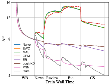
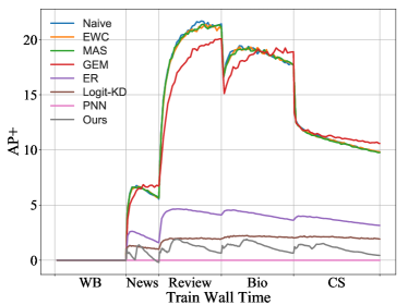
Figure 7: AP and $\text{AP}^{+}$ of different lifelong learning methods with $\text{BERT}_{\text{L6\_D384}}$ as the initial PLM w.r.t train wall time. ELLE continually grows $\text{BERT}_{\text{L6\_D384}}$ to $\text{BERT}_{\text{L12\_D768}}$.

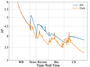
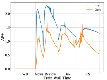
Figure 8: AP and $\text{AP}^{+}$ of ELLE when growing $\text{BERT}_{\text{L12\_D768}}$ to $\text{BERT}_{\text{L24\_D1024}}$.

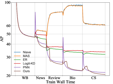
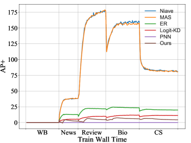
Figure 9: AP and $\text{AP}^{+}$ of different lifelong learning methods with $\text{GPT}_{\text{L6\_D384}}$ as the initial PLM w.r.t train wall time. ELLE continually grows $\text{GPT}_{\text{L6\_D384}}$ to $\text{GPT}_{\text{L12\_D768}}$.

For the experiments in § 4, the trend curves of average perplexity (AP) and average increased perplexity ($\text{AP}^{+}$) w.r.t train wall time are shown in Figure 7 (growing from $\text{BERT}_{\text{L6\_D384}}$ to $\text{BERT}_{\text{L12\_D768}}$), Figure 8 (growing from $\text{BERT}_{\text{L12\_D768}}$ to $\text{BERT}_{\text{L24\_D1024}}$), and Figure 9 (growing from $\text{GPT}_{\text{L6\_D384}}$ to $\text{GPT}_{\text{L12\_D768}}$). Each figure illustrates the performance of different lifelong learning methods. The above results reflect that, compared with all the baselines, AP and $\text{AP}^{+}$ of ELLE descend with the fastest speed, demonstrating that ELLE could acquire knowledge and mitigate the knowledge forgetting on previous domains more efficiently. Thus given limited computational resources, PLMs trained by ELLE could integrate more information from different domains.

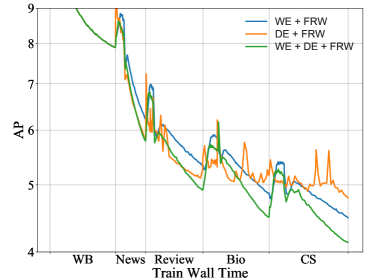
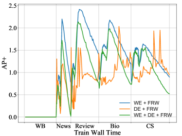
Figure 10: AP and $\text{AP}^{+}$ of PLMs trained with different model expansion strategies: expanding width only (WE+FRW), expanding depth only (DE+FRW) and expanding width and depth together (WE+DE+FRW) w.r.t train wall time.

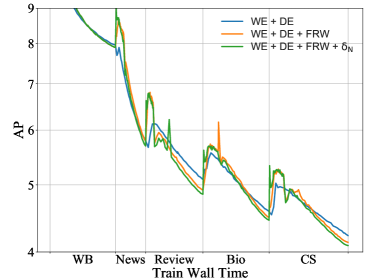
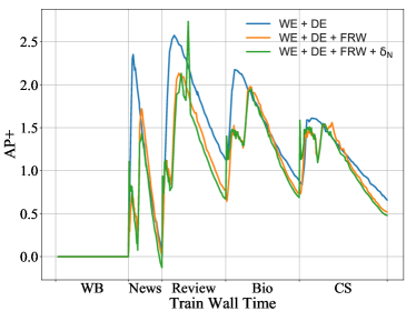
Figure 11: AP and $\text{AP}^{+}$ of PLMs trained by WE+DE, WE+DE+FRW, WE+DE+FRW+$\delta_{N}$ w.r.t train wall time.

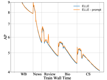
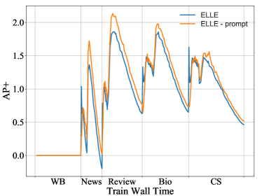
Figure 12: AP and $\text{AP}^{+}$ of PLMs trained by ELLE with and without domain prompts w.r.t train wall time.

For the analysis in § 5, we visualize the trend curves of AP and $\text{AP}^{+}$ when choosing different combinations of strategies. Specifically, we investigate (1) the effect of width / depth expansion in Figure 10 (comparing WE+FRW, DE+FRW and WE+DE+FRW); (2) the effect of function recovering warmup in Figure 11 (comparing WE+DE and WE+DE+FRW); (3) the effect of random noises added into the newly initialized parameters during model expansion in Figure 11 (comparing WE+DE+FRW and WE+DE+FRW+$\delta_{N}$) and (4) the effect of pre-trained domain prompts in Figure 12 (comparing ELLE and ELLE-PT). All of the above results again demonstrate the effectiveness of ELLE’s each component.

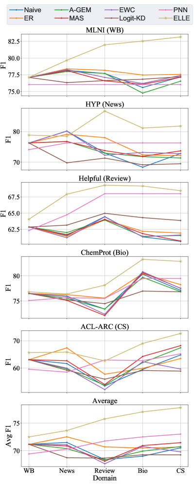
Figure 5: Specific and average F1 on downstream tasks of all domains of different lifelong learning methods. The initial PLM is chosen as $\text{BERT}_{\text{L6\_D384}}$. The score is evaluated after each model finishes training on each domain.

Domain	WB	Ns	Rev	Bio	CS	AVG
Naive
$\mathcal{M}_{1}$	$77.11$	$76.29$	$62.85$	$76.49$	$63.07$	$71.16$
$\mathcal{M}_{2}$	$78.17$	$80.21$	$61.54$	$75.95$	$61.64$	$71.50$
$\mathcal{M}_{3}$	$77.70$	$73.00$	$64.46$	$73.39$	$53.41$	$68.39$
$\mathcal{M}_{4}$	$75.60$	$68.33$	$61.32$	$80.32$	$59.49$	$69.01$
$\mathcal{M}_{5}$	$77.18$	$72.84$	$60.63$	$77.12$	$64.82$	$70.52$
A-GEM
$\mathcal{M}_{1}$	$77.11$	$76.29$	$62.85$	$76.49$	$63.07$	$71.16$
$\mathcal{M}_{2}$	$77.99$	$76.80$	$61.99$	$75.53$	$59.65$	$71.50$
$\mathcal{M}_{3}$	$77.71$	$72.96$	$63.92$	$73.39$	$53.66$	$68.39$
$\mathcal{M}_{4}$	$74.76$	$71.80$	$61.41$	$79.70$	$62.00$	$69.93$
$\mathcal{M}_{5}$	$76.55$	$71.37$	$61.53$	$76.85$	$64.82$	$70.75$
MAS
$\mathcal{M}_{1}$	$77.11$	$76.29$	$62.85$	$76.49$	$63.07$	$71.16$
$\mathcal{M}_{2}$	$78.13$	$76.75$	$61.68$	$75.12$	$62.69$	$70.87$
$\mathcal{M}_{3}$	$76.60$	$73.79$	$64.04$	$72.11$	$53.95$	$70.87$
$\mathcal{M}_{4}$	$76.09$	$71.90$	$61.83$	$80.62$	$64.26$	$70.94$
$\mathcal{M}_{5}$	$77.14$	$73.70$	$60.69$	$77.53$	$68.23$	$71.46$
MAS
$\mathcal{M}_{1}$	$77.11$	$76.29$	$62.85$	$76.49$	$63.07$	$71.16$
$\mathcal{M}_{2}$	$78.30$	$80.15$	$61.18$	$75.87$	$59.96$	$71.09$
$\mathcal{M}_{3}$	$77,11$	$72.26$	$64.41$	$72.37$	$52.07$	$67.64$
$\mathcal{M}_{4}$	$76.21$	$73.21$	$61.34$	$80.81$	$62.33$	$70.78$
$\mathcal{M}_{5}$	$77.41$	$72.79$	$61.62$	$77.49$	$59.62$	$69.79$
ER
$\mathcal{M}_{1}$	$77.11$	$76.29$	$62.85$	$76.49$	$63.07$	$71.16$
$\mathcal{M}_{2}$	$78.40$	$79.13$	$61.41$	$76.25$	$67.41$	$72.52$
$\mathcal{M}_{3}$	$78.18$	$78.04$	$63.98$	$75.57$	$57.53$	$70.70$
$\mathcal{M}_{4}$	$77.47$	$72.40$	$62.19$	$80.44$	$59.89$	$73.13$
$\mathcal{M}_{5}$	$77.57$	$72.15$	$61.92$	$78.25$	$63.49$	$70.68$
Logit-KD
$\mathcal{M}_{1}$	$77.11$	$79.29$	$62.85$	$76.49$	$64.07$	$71.16$
$\mathcal{M}_{2}$	$76.33$	$69.77$	$63.14$	$75.21$	$59.19$	$68.73$
$\mathcal{M}_{3}$	$76.63$	$71.32$	$64.97$	$74.46$	$55.91$	$68.66$
$\mathcal{M}_{4}$	$76.84$	$69.12$	$64.30$	$76.96$	$59.11$	$69.27$
$\mathcal{M}_{5}$	$77.21$	$69.48$	$63.86$	$76.82$	$58.87$	$69.25$
PNN
$\mathcal{M}_{1}$	$76.04$	$74.11$	$62.31$	$75.09$	$59.57$	$69.42$
$\mathcal{M}_{2}$	$76.04$	$76.30$	$64.74$	$75.65$	$59.19$	$70.24$
$\mathcal{M}_{3}$	$76.04$	$76.30$	$68.01$	$75.51$	$55.91$	$71.76$
$\mathcal{M}_{4}$	$76.04$	$76.30$	$68.01$	$79.46$	$59.11$	$72.51$
$\mathcal{M}_{5}$	$76.04$	$76.30$	$68.01$	$79.46$	$58.87$	$73.01$
ELLE
$\mathcal{M}_{1}$	$77.12$	$78.85$	$64.05$	$76.81$	$65.67$	$72.50$
$\mathcal{M}_{2}$	$79.67$	$78.48$	$67.93$	$76.38$	$65.84$	$73.66$
$\mathcal{M}_{3}$	$81.99$	$86.75$	$69.32$	$78.14$	$62.63$	$75.77$
$\mathcal{M}_{4}$	$82.55$	$81.18$	$69.19$	$83.27$	$69.03$	$77.04$
$\mathcal{M}_{5}$	$83.17$	$81.83$	$68.47$	$82.87$	$72.69$	$77.81$

Table 9: Specific and average F1 scores on downstream tasks from each domain after the PLM finishes training on each domain. We evaluate PLMs trained with different lifelong learning methods that choose $\text{BERT}_{\text{\L 6\_D384}}$ as the initial model $\mathcal{M}_{1}$.

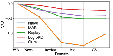
Figure 6: Average representational similarity (ARS) of a stream of PLMs comparing different lifelong learning algorithms. We choose $\text{BERT}_{\text{L6\_D384}}$ as the initial PLM $\mathcal{M}_{1}$.

Domain	WB		Ns		Rev		Bio		CS
Metrics	AP	AP+	AP	AP+	AP	AP+	AP	AP+	AP	AP+
Half train wall time
MAS	$7.96$	-	$8.50$	$6.22$	$12.85$	$18.88$	$13.99$	$17.52$	$10.31$	$10.22$
ER	$7.96$	-	$7.12$	$1.98$	$7.11$	$4.14$	$6.83$	$3.77$	$6.53$	$3.78$
Logit-KD	$7.96$	-	$7.72$	$1.12$	$7.27$	$1.94$	$7.17$	$2.08$	$7.06$	$1.99$
PNN	$7.96$	-	$6.75$	0.00	$5.53$	0.00	$5.09$	0.00	$5.03$	0.00
ELLE (ours)	7.92	-	6.05	$0.26$	5.21	$1.04$	4.83	$0.96$	4.42	$0.68$
Smaller memory
MAS	$7.96$	-	$8.08$	$5.65$	$13.44$	$21.17$	$13.87$	$17.67$	$9.91$	$9.75$
ER	$7.96$	-	$6.99$	$2.09$	$7.15$	$4.53$	$6.86$	$4.09$	$6.49$	$3.42$
Logit-KD	$7.96$	-	$7.68$	$1.15$	$7.24$	$2.06$	$7.21$	$2.27$	$7.05$	$2.16$
PNN	$7.96$	-	$6.52$	0.00	$5.29$	0.00	$4.84$	0.00	$4.76$	0.00
ELLE (ours)	7.92	-	5.85	$0.39$	5.04	$1.13$	4.58	$0.98$	4.20	$0.70$
Full train wall time & memory (the main results in § 4)
ELLE (ours)	$7.92$	-	$5.62$	$-0.20$	$4.81$	$0.64$	$4.41$	$0.64$	$4.06$	$0.44$

Table 10: Average perplexity (AP) and average increased perplexity ($\text{AP}^{+}$) of PLMs trained by different lifelong learning methods with half train wall time on Ns, Rev, Bio, CS domains and smaller memory containing $34$M tokens for each domain. We evaluate the performance each time when PLMs finish training on one domain.

Domain	WB	Ns	Rev	Bio	CS	AVG
Half train wall time
MAS	$76.7$	$72.3$	$61.6$	$77.4$	$64.3$	$70.5$
ER	$78.0$	$71.0$	$61.1$	$77.4$	$65.8$	$70.7$
Logit-KD	$77.0$	$72.6$	$63.8$	$76.2$	$58.4$	$69.6$
PNN	$76.0$	$55.9$	$62.6$	$53.1$	$28.0$	$55.1$
ELLE	82.0	78.4	68.7	81.7	74.0	77.0
Smaller memory
MAS	$77.1$	$73.7$	$60.7$	$77.5$	$68.2$	$71.5$
ER	$77.9$	$72.0$	$61.5$	$76.3$	$63.6$	$70.3$
Logit-KD	$77.0$	$73.1$	$63.3$	$75.9$	$57.4$	$69.3$
PNN	$76.0$	$64.9$	$64.2$	$55.1$	$30.5$	$58.1$
ELLE	82.9	80.5	68.9	82.6	74.2	77.8
Full train wall time & memory (the main results in § 4)
ELLE	$83.2$	$81.8$	$68.5$	$82.9$	$72.7$	$77.8$

Table 11: Final downstream performance (F1) of BERT on each domain after finishing pre-training on all domains with half train wall time on Ns, Rev, Bio, CS domains and smaller memory containing $34$M tokens for each domain. Experiments of Ns domain are repeated for $10$ times with different seeds and others are repeated for $5$ times.

Model	$n_{\text{params}}$	$n_{\text{layers}}$	$d_{\text{model}}$	$n_{\text{heads}}$	$d_{\text{FFN}}$	lr
WE + FRW
$\mathcal{M}_{1}$	$30.3$M	$6$	$384$	$6$	$1536$	$5.0\times 10^{-4}$
$\mathcal{M}_{2}$	$53.6$M	$6$	$576$	$9$	$2304$	$5.0\times 10^{-4}$
$\mathcal{M}_{3}$	$82.2$M	$6$	$768$	$12$	$3072$	$5.0\times 10^{-4}$
$\mathcal{M}_{4}$	$104$M	$6$	$896$	$14$	$3584$	$5.0\times 10^{-4}$
$\mathcal{M}_{5}$	$129$M	$6$	$1024$	$16$	$4096$	$5.0\times 10^{-4}$
DE + FRW
$\mathcal{M}_{1}$	$30.3$M	$12$	$768$	$12$	$3072$	$5.0\times 10^{-4}$
$\mathcal{M}_{2}$	$51.6$M	$18$	$768$	$12$	$3072$	$2.5\times 10^{-4}$
$\mathcal{M}_{3}$	$83.6$M	$36$	$768$	$12$	$3072$	$2.5\times 10^{-4}$
$\mathcal{M}_{4}$	$105$M	$48$	$768$	$12$	$3072$	$2.5\times 10^{-4}$
$\mathcal{M}_{5}$	$126$M	$60$	$768$	$12$	$3072$	$2.5\times 10^{-4}$
WE + DE + FRW
$\mathcal{M}_{1}$	$30.3$M	$6$	$384$	$6$	$1536$	$5.0\times 10^{-4}$
$\mathcal{M}_{2}$	$51.5$M	$8$	$512$	$8$	$2048$	$5.0\times 10^{-4}$
$\mathcal{M}_{3}$	$82.2$M	$10$	$640$	$10$	$2560$	$5.0\times 10^{-4}$
$\mathcal{M}_{4}$	$102$M	$11$	$704$	$11$	$2816$	$5.0\times 10^{-4}$
$\mathcal{M}_{5}$	$125$M	$12$	$768$	$12$	$3072$	$5.0\times 10^{-4}$

Table 12: Model architectures the investigated PLMs of WE+FRW, DE+FRW, WE+DE+FRW. We keep the total number of $\mathcal{M}_{i}$’s increased parameters for the above three strategies almost the same at each stage $i$.

Appendix E Representational Similarity of a Stream of PLMs

We investigate the representational similarity (Abnar et al., 2019) of a descendant PLM and its ancestors. Representational similarity measures how similar two PLMs represent the data. Specifically, we experiment on a stream of PLMs when growing $\text{BERT}_{\text{L6\_D384}}$ to $\text{BERT}_{\text{L12\_D768}}$. For a model $\mathcal{M}_{j}$ and its ancestor $\mathcal{M}_{i}$ ($1\leq i\leq j-1$), we randomly sample $n$ [MASK] tokens from the raw corpus $\mathcal{D}_{j}$, and get the probability distributions $\bm{p}_{k}^{i}$ and $\bm{p}_{k}^{j}$ output by the LM head of $\mathcal{M}_{i}$ and $\mathcal{M}_{j}$, respectively for each [MASK] token $k$, where $1\leq k\leq n$. We calculate the average representational similarity (ARS) between $\mathcal{M}_{j}$ and all its ancestors $\{\mathcal{M}_{1},\cdots,\mathcal{M}_{j-1}\}$ as follows:

$$\text{ARS}_{j} =\frac{-1}{(j-1)\times n}\sum_{i=1}^{j-1}\sum_{k=1}^{n}\text{KL}(\bm{p}_{k}^{i},\bm{p}_{k}^{j}),$$ (4)

where KL denotes the Kullback-Leibler divergence between two probability distributions. Higher $\text{ARS}_{j}$ means the representations of $\mathcal{M}_{j}$ and its ancestors are more similar. To some extent, $\text{ARS}_{j}$ could reflect how much knowledge / functionality of the ancestors is preserved by $\mathcal{M}_{j}$.

We compare ARS of PLMs trained by Naive, MAS, ER, Logit-KD and ELLE and illustrate the results in Figure 6, from which we observe that Logit-KD has the highest ARS. This is because the training objective of knowledge distillation in Logit-KD is highly correlated with ARS. In addition, ELLE takes second place. We also find that, with PLMs continually absorbing new knowledge, the ASR generally decreases.

Appendix F Model Architectures for the Analysis of Model Expansion

In Table 12, we list the model architectures of all the investigated PLMs when conducting the analysis of model expansion in § 5. Specifically, three strategies are investigated, including WE+FRW, DE+FRW and WE+DE+FRW. As mentioned in our main paper, for a fair comparison, we keep the total number of $\mathcal{M}_{i}$’s increased parameters for the above three strategies almost the same at each stage $i$.

Appendix G Performance of ELLE with Fewer Computational Budgets and Storage Budgets

To investigate the performance of ELLE under limited (1) computational budgets and (2) storage budgets, in this section, we take an initial step to investigate the effect of (1) training resources (train wall time) and (2) memory size for ELLE. Following the experimental setting in § 4, we continually grow $\text{BERT}_{\text{L6\_D384}}$ to $\text{BERT}_{\text{L12\_D768}}$ on a stream of data from $5$ domains. We test the performance of ELLE and a series of lifelong learning baselines (MAS, ER, Logit-KD and PNN), by (1) reducing the train wall time by half (for Ns, Rev, Bio and CS domain) and (2) randomly sample only $34$M tokens ($1$% of the full corpus) as the memory $\mathcal{D}_{i}^{sub}$ for each corpus $i$, compared with the memory size $200$M in § 4.

The experimental results for the above two settings are listed in Table 10 (pre-training) and Table 11 (fine-tuning), respectively. We also illustrate the trend curves of AP and $\text{AP}^{+}$ in Figure 13 and Figure 14. From the above results, we find that: (1) when given fewer computational budgets and storage budgets, ELLE still outperforms all the lifelong learning baselines in both pre-training and downstream performance, which demonstrates the superiority of ELLE; (2) for ELLE, when PLMs are trained with fewer computational budgets, we observe significant performance drops in both pre-training (higher AP and $\text{AP}^{+}$) and downstream tasks (lower average F1). This shows that pre-training with fewer computations would harm PLMs’ knowledge acquisition; (3) for ELLE, when there are fewer memory budgets, although we also observe slight performance drops in pre-training (higher AP and $\text{AP}^{+}$), the performance in downstream tasks is generally not influenced, with the average F1 score keeping almost the same ($77.8$). This shows the data-efficiency of PLMs, i.e., PLMs could easily recall the learned knowledge by reviewing small-scale data conserved in the memory (as few as $1\%$). As mentioned before, considering that for pre-training, the expense of storage (e.g., hard disks) is far cheaper than the computational resources (e.g., GPUs), the storage space problem for memory seldom needs to be considered.

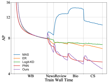
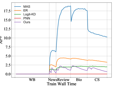
Figure 13: AP and $\text{AP}^{+}$ of different lifelong learning methods with $\text{BERT}_{\text{L6\_D384}}$ as the initial model w.r.t train wall time. The train wall time on News, Review, Bio, CS domains is half of the original experiment in Section 4. ELLE continually grows $\text{BERT}_{\text{L6\_D384}}$ to $\text{BERT}_{\text{L12\_D768}}$.

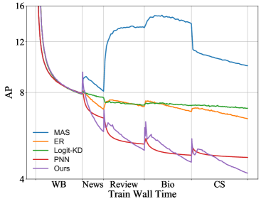
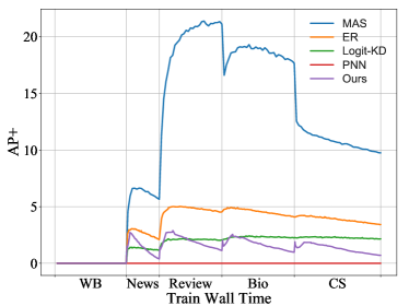
Figure 14: AP and $\text{AP}^{+}$ of different lifelong learning methods with $\text{BERT}_{\text{L6\_D384}}$ as the initial model with smaller memory w.r.t train wall time. For domain $i$, we randomly sample only about $34$M tokens as memory $\mathcal{D}_{i}^{sub}$, which is $1\%$ of training corpus $\mathcal{D}_{i}$ . ELLE continually grows $\text{BERT}_{\text{L6\_D384}}$ to $\text{BERT}_{\text{L12\_D768}}$.

Appendix H Details of Baselines

We tried different hyper-parameters for baselines, including the regularization parameter $\lambda$ for EWC and MAS, and the memory size for A-GEM, to derive and report their best performance. Their AP and $\text{AP}^{+}$ curves are shown in Figure 15, 16 and 17. From the results we can see that none of these hyperparameters works well. For EWC and MAS, when the regularization parameter $\lambda$ is small, the pre-training performance is not better than that of naive method. However, if we slightly increase $\lambda$, the performance would become worse than baseline. For A-GEM, the case with bigger memory also doesn’t outperform cases with smaller memory and naive case. Specially, we observed that during A-GEM pre-training, $99.9$% of the inter-products of current gradient and replay gradient are positive, implying that pre-training on different domains is similar to each other to a large extent. This might indicate that EWC, MAS, and A-GEM cannot deal with the subtle difference of various domains.

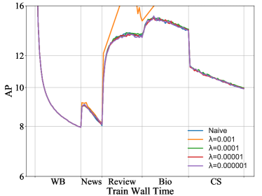
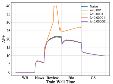
Figure 15: AP and $\text{AP}^{+}$ of EWC with $\text{BERT}_{\text{L6\_D384}}$ as the initial model and with different regularization parameter $\lambda$ w.r.t train wall time.

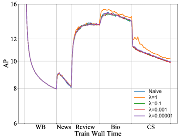
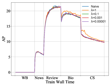
Figure 16: AP and $\text{AP}^{+}$ of MAS with $\text{BERT}_{\text{L6\_D384}}$ as the initial model and with different regularization parameter $\lambda$ w.r.t train wall time.

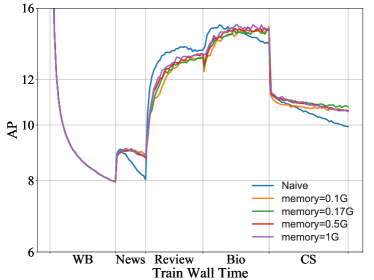
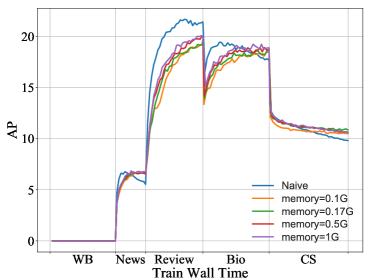
Figure 17: AP and $\text{AP}^{+}$ of GEM with $\text{BERT}_{\text{L6\_D384}}$ as the initial model and with different memory size w.r.t train wall time.

References

- Abnar et al. (2019) Samira Abnar, Lisa Beinborn, Rochelle Choenni, and Willem Zuidema. 2019. Blackbox meets blackbox: Representational similarity and stability analysis of neural language models and brains. ArXiv preprint, abs/1906.01539.
- Aljundi et al. (2018) Rahaf Aljundi, Francesca Babiloni, Mohamed Elhoseiny, Marcus Rohrbach, and Tinne Tuytelaars. 2018. Memory aware synapses: Learning what (not) to forget. In Proceedings of the European Conference on Computer Vision (ECCV).
- Arora et al. (2018) Sanjeev Arora, Nadav Cohen, and Elad Hazan. 2018. On the optimization of deep networks: Implicit acceleration by overparameterization. In Proceedings of the 35th International Conference on Machine Learning, ICML 2018, Stockholmsmässan, Stockholm, Sweden, July 10-15, 2018, volume 80 of Proceedings of Machine Learning Research, pages 244–253. PMLR.
- Chaudhry et al. (2019a) Arslan Chaudhry, Marc’Aurelio Ranzato, Marcus Rohrbach, and Mohamed Elhoseiny. 2019a. Efficient lifelong learning with A-GEM. In 7th International Conference on Learning Representations, ICLR 2019, New Orleans, LA, USA, May 6-9, 2019. OpenReview.net.
- Chaudhry et al. (2019b) Arslan Chaudhry, Marcus Rohrbach, Mohamed Elhoseiny, Thalaiyasingam Ajanthan, Puneet K Dokania, Philip HS Torr, and Marc’Aurelio Ranzato. 2019b. On tiny episodic memories in continual learning. ArXiv preprint, abs/1902.10486.
- Chen et al. (2021) Cheng Chen, Yichun Yin, Lifeng Shang, Xin Jiang, Yujia Qin, Fengyu Wang, Zhi Wang, Xiao Chen, Zhiyuan Liu, and Qun Liu. 2021. bert2bert: Towards reusable pretrained language models. ArXiv preprint, abs/2110.07143.
- Clark et al. (2020) Kevin Clark, Minh-Thang Luong, Quoc V. Le, and Christopher D. Manning. 2020. ELECTRA: pre-training text encoders as discriminators rather than generators. In 8th International Conference on Learning Representations, ICLR 2020, Addis Ababa, Ethiopia, April 26-30, 2020. OpenReview.net.
- de Masson d’Autume et al. (2019) Cyprien de Masson d’Autume, Sebastian Ruder, Lingpeng Kong, and Dani Yogatama. 2019. Episodic memory in lifelong language learning. In Advances in Neural Information Processing Systems 32: Annual Conference on Neural Information Processing Systems 2019, NeurIPS 2019, December 8-14, 2019, Vancouver, BC, Canada, pages 13122–13131.
- Devlin et al. (2019) Jacob Devlin, Ming-Wei Chang, Kenton Lee, and Kristina Toutanova. 2019. BERT: Pre-training of deep bidirectional transformers for language understanding. In Proceedings of the 2019 Conference of the North American Chapter of the Association for Computational Linguistics: Human Language Technologies, Volume 1 (Long and Short Papers), pages 4171–4186, Minneapolis, Minnesota. Association for Computational Linguistics.
- Dhingra et al. (2021) Bhuwan Dhingra, Jeremy R Cole, Julian Martin Eisenschlos, Daniel Gillick, Jacob Eisenstein, and William W Cohen. 2021. Time-aware language models as temporal knowledge bases. ArXiv preprint, abs/2106.15110.
- Gong et al. (2019) Linyuan Gong, Di He, Zhuohan Li, Tao Qin, Liwei Wang, and Tie-Yan Liu. 2019. Efficient training of BERT by progressively stacking. In Proceedings of the 36th International Conference on Machine Learning, ICML 2019, 9-15 June 2019, Long Beach, California, USA, volume 97 of Proceedings of Machine Learning Research, pages 2337–2346. PMLR.
- Gu et al. (2021) Xiaotao Gu, Liyuan Liu, Hongkun Yu, Jing Li, Chen Chen, and Jiawei Han. 2021. On the transformer growth for progressive BERT training. In Proceedings of the 2021 Conference of the North American Chapter of the Association for Computational Linguistics: Human Language Technologies, pages 5174–5180, Online. Association for Computational Linguistics.
- Gururangan et al. (2021) Suchin Gururangan, Mike Lewis, Ari Holtzman, Noah A Smith, and Luke Zettlemoyer. 2021. Demix layers: Disentangling domains for modular language modeling. ArXiv preprint, abs/2108.05036.
- Gururangan et al. (2020) Suchin Gururangan, Ana Marasović, Swabha Swayamdipta, Kyle Lo, Iz Beltagy, Doug Downey, and Noah A. Smith. 2020. Don’t stop pretraining: Adapt language models to domains and tasks. In Proceedings of the 58th Annual Meeting of the Association for Computational Linguistics, pages 8342–8360, Online. Association for Computational Linguistics.
- Han et al. (2021) Xu Han, Zhengyan Zhang, Ning Ding, Yuxian Gu, Xiao Liu, Yuqi Huo, Jiezhong Qiu, Liang Zhang, Wentao Han, Minlie Huang, Qin Jin, Yanyan Lan, Yang Liu, Zhiyuan Liu, Zhiwu Lu, Xipeng Qiu, Ruihua Song, Jie Tang, Ji-Rong Wen, Jinhui Yuan, Wayne Xin Zhao, and Jun Zhu. 2021. Pre-trained models: Past, present and future. ArXiv preprint, abs/2106.07139.
- He et al. (2021) Ruidan He, Linlin Liu, Hai Ye, Qingyu Tan, Bosheng Ding, Liying Cheng, Jiawei Low, Lidong Bing, and Luo Si. 2021. On the effectiveness of adapter-based tuning for pretrained language model adaptation. In Proceedings of the 59th Annual Meeting of the Association for Computational Linguistics and the 11th International Joint Conference on Natural Language Processing (Volume 1: Long Papers), pages 2208–2222, Online. Association for Computational Linguistics.
- He and McAuley (2016) Ruining He and Julian J. McAuley. 2016. Ups and downs: Modeling the visual evolution of fashion trends with one-class collaborative filtering. In Proceedings of the 25th International Conference on World Wide Web, WWW 2016, Montreal, Canada, April 11 - 15, 2016, pages 507–517. ACM.
- Jang et al. (2021) Joel Jang, Seonghyeon Ye, Sohee Yang, Joongbo Shin, Janghoon Han, Gyeonghun Kim, Stanley Jungkyu Choi, and Minjoon Seo. 2021. Towards continual knowledge learning of language models. ArXiv preprint, abs/2110.03215.
- Jin et al. (2021) Xisen Jin, Dejiao Zhang, Henghui Zhu, Wei Xiao, Shang-Wen Li, Xiaokai Wei, Andrew Arnold, and Xiang Ren. 2021. Lifelong pretraining: Continually adapting language models to emerging corpora. ArXiv preprint, abs/2110.08534.
- Jurgens et al. (2018) David Jurgens, Srijan Kumar, Raine Hoover, Dan McFarland, and Dan Jurafsky. 2018. Measuring the evolution of a scientific field through citation frames. Transactions of the Association for Computational Linguistics, 6:391–406.
- Kaplan et al. (2020) Jared Kaplan, Sam McCandlish, Tom Henighan, Tom B Brown, Benjamin Chess, Rewon Child, Scott Gray, Alec Radford, Jeffrey Wu, and Dario Amodei. 2020. Scaling laws for neural language models. ArXiv preprint, abs/2001.08361.
- Kiesel et al. (2019) Johannes Kiesel, Maria Mestre, Rishabh Shukla, Emmanuel Vincent, Payam Adineh, David Corney, Benno Stein, and Martin Potthast. 2019. SemEval-2019 task 4: Hyperpartisan news detection. In Proceedings of the 13th International Workshop on Semantic Evaluation, pages 829–839, Minneapolis, Minnesota, USA. Association for Computational Linguistics.
- Kingma and Ba (2015) Diederik P. Kingma and Jimmy Ba. 2015. Adam: A method for stochastic optimization. In 3rd International Conference on Learning Representations, ICLR 2015, San Diego, CA, USA, May 7-9, 2015, Conference Track Proceedings.
- Kirkpatrick et al. (2017) James Kirkpatrick, Razvan Pascanu, Neil Rabinowitz, Joel Veness, Guillaume Desjardins, Andrei A Rusu, Kieran Milan, John Quan, Tiago Ramalho, Agnieszka Grabska-Barwinska, et al. 2017. Overcoming catastrophic forgetting in neural networks. Proceedings of the national academy of sciences, 114(13):3521–3526.
- Kringelum et al. (2016) Jens Kringelum, Sonny Kim Kjaerulff, Søren Brunak, Ole Lund, Tudor I Oprea, and Olivier Taboureau. 2016. Chemprot-3.0: a global chemical biology diseases mapping. Database, 2016.
- Li et al. (2020) Zhuohan Li, Eric Wallace, Sheng Shen, Kevin Lin, Kurt Keutzer, Dan Klein, and Joey Gonzalez. 2020. Train big, then compress: Rethinking model size for efficient training and inference of transformers. In Proceedings of the 37th International Conference on Machine Learning, ICML 2020, 13-18 July 2020, Virtual Event, volume 119 of Proceedings of Machine Learning Research, pages 5958–5968. PMLR.
- Lo et al. (2020) Kyle Lo, Lucy Lu Wang, Mark Neumann, Rodney Kinney, and Daniel Weld. 2020. S2ORC: The semantic scholar open research corpus. In Proceedings of the 58th Annual Meeting of the Association for Computational Linguistics, pages 4969–4983, Online. Association for Computational Linguistics.
- Lopez-Paz and Ranzato (2017) David Lopez-Paz and Marc’Aurelio Ranzato. 2017. Gradient episodic memory for continual learning. In Advances in Neural Information Processing Systems 30: Annual Conference on Neural Information Processing Systems 2017, December 4-9, 2017, Long Beach, CA, USA, pages 6467–6476.
- McAuley et al. (2015) Julian J. McAuley, Christopher Targett, Qinfeng Shi, and Anton van den Hengel. 2015. Image-based recommendations on styles and substitutes. In Proceedings of the 38th International ACM SIGIR Conference on Research and Development in Information Retrieval, Santiago, Chile, August 9-13, 2015, pages 43–52. ACM.
- McCloskey and Cohen (20p) Michael McCloskey and Neal J Cohen. 20p. Catastrophic interference in connectionist networks: The sequential learning problem. ArXiv preprint, abs/p.
- Ott et al. (2019) Myle Ott, Sergey Edunov, Alexei Baevski, Angela Fan, Sam Gross, Nathan Ng, David Grangier, and Michael Auli. 2019. fairseq: A fast, extensible toolkit for sequence modeling. In Proceedings of the 2019 Conference of the North American Chapter of the Association for Computational Linguistics (Demonstrations), pages 48–53, Minneapolis, Minnesota. Association for Computational Linguistics.
- Qin et al. (2021a) Yujia Qin, Yankai Lin, Jing Yi, Jiajie Zhang, Xu Han, Zhengyan Zhang, Yusheng Su, Zhiyuan Liu, Peng Li, Maosong Sun, et al. 2021a. Knowledge inheritance for pre-trained language models. ArXiv preprint, abs/2105.13880.
- Qin et al. (2021b) Yujia Qin, Xiaozhi Wang, Yusheng Su, Yankai Lin, Ning Ding, Zhiyuan Liu, Juanzi Li, Lei Hou, Peng Li, Maosong Sun, et al. 2021b. Exploring low-dimensional intrinsic task subspace via prompt tuning. ArXiv preprint, abs/2110.07867.
- Radford et al. (2018) Alec Radford, Karthik Narasimhan, Tim Salimans, and Ilya Sutskever. 2018. Improving language understanding by generative pre-training.
- Rebuffi et al. (2017) Sylvestre-Alvise Rebuffi, Alexander Kolesnikov, Georg Sperl, and Christoph H. Lampert. 2017. icarl: Incremental classifier and representation learning. In 2017 IEEE Conference on Computer Vision and Pattern Recognition, CVPR 2017, Honolulu, HI, USA, July 21-26, 2017, pages 5533–5542. IEEE Computer Society.
- Rolnick et al. (2019) David Rolnick, Arun Ahuja, Jonathan Schwarz, Timothy P. Lillicrap, and Gregory Wayne. 2019. Experience replay for continual learning. In Advances in Neural Information Processing Systems 32: Annual Conference on Neural Information Processing Systems 2019, NeurIPS 2019, December 8-14, 2019, Vancouver, BC, Canada, pages 348–358.
- Rusu et al. (2016) Andrei A Rusu, Neil C Rabinowitz, Guillaume Desjardins, Hubert Soyer, James Kirkpatrick, Koray Kavukcuoglu, Razvan Pascanu, and Raia Hadsell. 2016. Progressive neural networks. ArXiv preprint, abs/1606.04671.
- Schwartz et al. (2019) Roy Schwartz, Jesse Dodge, Noah A Smith, and Oren Etzioni. 2019. Green ai. ArXiv preprint, abs/1907.10597.
- Schwarz et al. (2018) Jonathan Schwarz, Wojciech Czarnecki, Jelena Luketina, Agnieszka Grabska-Barwinska, Yee Whye Teh, Razvan Pascanu, and Raia Hadsell. 2018. Progress & compress: A scalable framework for continual learning. In Proceedings of the 35th International Conference on Machine Learning, ICML 2018, Stockholmsmässan, Stockholm, Sweden, July 10-15, 2018, volume 80 of Proceedings of Machine Learning Research, pages 4535–4544. PMLR.
- Shazeer et al. (2018) Noam Shazeer, Youlong Cheng, Niki Parmar, Dustin Tran, Ashish Vaswani, Penporn Koanantakool, Peter Hawkins, HyoukJoong Lee, Mingsheng Hong, Cliff Young, Ryan Sepassi, and Blake A. Hechtman. 2018. Mesh-tensorflow: Deep learning for supercomputers. In Advances in Neural Information Processing Systems 31: Annual Conference on Neural Information Processing Systems 2018, NeurIPS 2018, December 3-8, 2018, Montréal, Canada, pages 10435–10444.
- Shoeybi et al. (2019) Mohammad Shoeybi, Mostofa Patwary, Raul Puri, Patrick LeGresley, Jared Casper, and Bryan Catanzaro. 2019. Megatron-lm: Training multi-billion parameter language models using model parallelism. ArXiv preprint, abs/1909.08053.
- Su et al. (2021) Yusheng Su, Xiaozhi Wang, Yujia Qin, Chi-Min Chan, Yankai Lin, Zhiyuan Liu, Peng Li, Juanzi Li, Lei Hou, Maosong Sun, et al. 2021. On transferability of prompt tuning for natural language understanding. ArXiv preprint, abs/2111.06719.
- Sun et al. (2020) Fan-Keng Sun, Cheng-Hao Ho, and Hung-Yi Lee. 2020. LAMOL: language modeling for lifelong language learning. In 8th International Conference on Learning Representations, ICLR 2020, Addis Ababa, Ethiopia, April 26-30, 2020. OpenReview.net.
- Vaswani et al. (2017) Ashish Vaswani, Noam Shazeer, Niki Parmar, Jakob Uszkoreit, Llion Jones, Aidan N. Gomez, Lukasz Kaiser, and Illia Polosukhin. 2017. Attention is all you need. In Advances in Neural Information Processing Systems 30: Annual Conference on Neural Information Processing Systems 2017, December 4-9, 2017, Long Beach, CA, USA, pages 5998–6008.
- Williams et al. (2018) Adina Williams, Nikita Nangia, and Samuel Bowman. 2018. A broad-coverage challenge corpus for sentence understanding through inference. In Proceedings of the 2018 Conference of the North American Chapter of the Association for Computational Linguistics: Human Language Technologies, Volume 1 (Long Papers), pages 1112–1122, New Orleans, Louisiana. Association for Computational Linguistics.
- Wu et al. (2021) Tongtong Wu, Massimo Caccia, Zhuang Li, Yuan-Fang Li, Guilin Qi, and Gholamreza Haffari. 2021. Pretrained language model in continual learning: A comparative study. In International Conference on Learning Representations.
- Yoon et al. (2018) Jaehong Yoon, Eunho Yang, Jeongtae Lee, and Sung Ju Hwang. 2018. Lifelong learning with dynamically expandable networks. In 6th International Conference on Learning Representations, ICLR 2018, Vancouver, BC, Canada, April 30 - May 3, 2018, Conference Track Proceedings. OpenReview.net.
- You et al. (2020) Yang You, Jing Li, Sashank J. Reddi, Jonathan Hseu, Sanjiv Kumar, Srinadh Bhojanapalli, Xiaodan Song, James Demmel, Kurt Keutzer, and Cho-Jui Hsieh. 2020. Large batch optimization for deep learning: Training BERT in 76 minutes. In 8th International Conference on Learning Representations, ICLR 2020, Addis Ababa, Ethiopia, April 26-30, 2020. OpenReview.net.
- Zellers et al. (2019) Rowan Zellers, Ari Holtzman, Hannah Rashkin, Yonatan Bisk, Ali Farhadi, Franziska Roesner, and Yejin Choi. 2019. Defending against neural fake news. In Advances in Neural Information Processing Systems 32: Annual Conference on Neural Information Processing Systems 2019, NeurIPS 2019, December 8-14, 2019, Vancouver, BC, Canada, pages 9051–9062.
- Zhang and He (2020) Minjia Zhang and Yuxiong He. 2020. Accelerating training of transformer-based language models with progressive layer dropping. ArXiv preprint, abs/2010.13369.
- Zhu et al. (2015) Yukun Zhu, Ryan Kiros, Richard S. Zemel, Ruslan Salakhutdinov, Raquel Urtasun, Antonio Torralba, and Sanja Fidler. 2015. Aligning books and movies: Towards story-like visual explanations by watching movies and reading books. In 2015 IEEE International Conference on Computer Vision, ICCV 2015, Santiago, Chile, December 7-13, 2015, pages 19–27. IEEE Computer Society.