Island and Page curve for one-sided asymptotically flat black hole

Abstract

Great breakthrough in solving black hole information paradox took place when semiclassical island rule for entanglement entropy of Hawking radiation was proposed in recent years. Up to now, most papers which discussed island rule of asymptotic flat black hole with $D\geq 4$ focus on eternal black hole. In this paper, we take one more step further by discussing island of “in” vacuum state which describes one-sided asymptotically flat black hole formed by gravitational collapse in $D\geq 4$. We find that island $I$ emerges at late time and saves entropy bound. And boundary of island $\partial I$ depends on the position of cutoff surface. When cutoff surface is far from horizon, $\partial I$ is inside and near horizon. When cutoff surface is set to be near horizon, $\partial I$ is outside and near horizon. This is different from the case of eternal black hole in which $\partial I$ is always outside horizon no matter cutoff surface is far from or near horizon. We will see that different states will manifestly affect $S_{\text{ent}}$ in island formula when cutoff surface is far from horizon and thus have different result for Page time.

I Introduction

Black hole information paradox is a long lasting debate over more than 40 years since Hawking discovered that information may be lost in evaporation of black hole Hawking:1976ra . Hawking’s calculation implies that von Newman entropy of Hawking radiation will increase monotonically. On the other hand, quantum mechanics requires black hole evaporation to be unitary, thus von Newman entropy of Hawking radiation should obey Page curve if information is preserved during black hole evaporation Page:1993wv . Since then, producing Page curve in gravitational calculation is a key step towards solving information paradox.

In Penington:2019npb ; Almheiri:2019psf ; Almheiri:2019hni , island rule is proposed to calculate Page curve of Hawking radiation (see e.g. Almheiri:2020cfm for a review). Island rule states that fine grained entropy of black hole is given by

$$S(BH)=\text{min}\left\{\text{ext}\left[\frac{\text{Area}(\partial I)}{4G_{N}}+S_{\text{ent}}(B)\right]\right\},$$ (1.1)

and fine grained entropy of Hawking radiation is given by

$$S(R)=\text{min}\left\{\text{ext}\left[\frac{\text{Area}(\partial I)}{4G_{N}}+S_{\text{ent}}(I\cup R)\right]\right\},$$ (1.2)

where $R$ denotes the region outside cutoff surface $A$ and collecting Hawking radiation, $I$ is called island and denotes an codimension-one hypersurface which penetrates into the interior of black hole, $\partial I$ is the codimension-two boundary of $I$ (see fig.(1)). $\partial I$ is chosen to be the quantum extremal surface (QES) Engelhardt:2014gca that extremizes the generalized entropy Faulkner:2013ana ; Lewkowycz:2013nqa ; Dong:2016hjy

$$S_{\text{gen}}=\frac{\text{Area}(\partial I)}{4G_{N}}+S_{\text{ent}},$$ (1.3)

where the first term is area term from Ryu-Takayanagi formula Ryu:2006bv ; Hubeny:2007xt , and the second term is coarse-grained entropy of matter fields. If there are more than one extremal surface, the global minimum one should be taken. This is the meaning of “min” and “ext” in eq.(1.1) and eq.(1.2). Island formula can be derived by using replica trick to construct replica wormhole Penington:2019kki ; Almheiri:2019qdq .

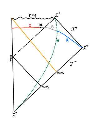
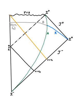
(a)	(b)

Figure 1: (a) The Penrose diagram for one-sided black hole formed by spherical null shell collapsing at $v=v_{0}$ (orange line) Fabbri:2005mw . Observer on cutoff surface $A$ (green dashed line) collects Hawking radiation in region $R$. Island (red line) penetrates into interior of black hole. $\partial I$ is quantum extremal surface. $I\cup B\cup R$ is a Cauchy slice. (b) Without island, we can equivalently fix $r_{I}=0$ and $t_{I}$ as some constant.

Island formula was discussed in Almheiri:2019psf ; Almheiri:2019hni ; Chen:2019uhq for $2D$ Jackiw-Teitelboim (JT) gravity in asymptotically anti-de Sitter (AdS) spacetimes coupled to a thermal bath, in Balasubramanian:2020xqf ; Geng:2021wcq for de Sitter (dS), in Hu:2022ymx for curvature-squared gravity, in Ling:2020laa for charged black holes, and in Almheiri:2019psy for higher dimensions. And the case for asymptotically flat spacetimes was discussed in Gautason:2020tmk ; Anegawa:2020ezn ; Hartman:2020swn ; Yu:2021cgi for dilaton gravity, in Azarnia:2021uch for flat-space cosmology, in Wang:2021mqq for a family of $2D$ exactly solvable black holes, in Alishahiha:2020qza ; Hashimoto:2020cas ; Matsuo:2020ypv ; Arefeva:2021kfx ; Dong:2020uxp for Schwarzschild black hole, in Kim:2021gzd ; Wang:2021woy for Reissner-Nordström black hole and in He:2021mst for a family of eternal black holes. Due to rapid progress in this field, above is only an incomplete list of references.

Up to now, as far as we know, most of the papers that discuss Schwarzschild black hole Alishahiha:2020qza ; Hashimoto:2020cas ; Matsuo:2020ypv ; Arefeva:2021kfx ; Dong:2020uxp and Reissner-Nordström black hole Kim:2021gzd ; Wang:2021woy only concern about eternal black hole and static vacuum Matsuo:2021mmi . In Alishahiha:2020qza , the authors discuss one-sided dynamical black hole but they implicitly assume Hartle-Hawking state Hartle:1976tp which is more appropriate to eternal black hole. Hartle-Hawking state or Hartle-Hawking vacuum is the unique state which is regular in the whole Kruskal extension of Schwarzschild black hole and is invariant under Schwarzschild time translation. It represents a black hole in thermal equilibrium with an outgoing Hawking radiation reaching future null infinity $\mathcal{J}^{+}$ and an equal incoming thermal radiation coming in from past null infinity $\mathcal{J}^{-}$.

In this paper, we will discuss “in” vacuum state which describes one-sided dynamic asymptotically flat black hole formed from collapsing of spherical null shell (see fig.(1)) Fabbri:2005mw . It can be approximated by Unruh state in late time limit. “In” vacuum state and Unruh state both can describe black hole formed by gravitational collapse since they both contain no incoming flux from $\mathcal{J}^{-}$. Hence, it is generally believed that, compared with the Hartle-Hawking state, “in” vacuum state is more appropriate to one-sided dynamic black hole. We will see that different state will manifestly affect $S_{\text{ent}}$ in island formula and thus have different result for Page time. In addition, different from Hartle-Hawking state for eternal black hole, due to absence of incoming flux, $s$-wave approximation is valid for “in” vacuum state of one-sided black hole formed from collapsing of spherical null shell when cutoff surface $A$ is far from horizon (see Appendix A). The use of “in” vacuum state is the key difference between our paper and the other papers that use Hartle-Hawking state Alishahiha:2020qza ; Hashimoto:2020cas ; Matsuo:2020ypv ; Arefeva:2021kfx ; Kim:2021gzd ; Wang:2021woy ; He:2021mst ; Matsuo:2021mmi .

This paper is organized as follows. In Sec. II, entanglement entropy $S_{\text{ent}}$ is discussed and we will see its dependence on state. In Sec. III, we discuss the case in which cutoff surface is far from horizon and find that boundary of island $\partial I$ is inside black hole horizon and produce the Page curve. In Sec. IV, we discuss the case in which cutoff surface is near horizon and find that boundary of island $\partial I$ is outside black hole horizon and produce the Page curve. In Sec. V, we discuss the case for higher dimensional ($D>4$) black hole formed by collapse of spherical null shell and find similar results as the $4D$ case. The conclusion and discussion are in Sec. VI.

II Entanglement entropy in black hole background

In this paper, we will mainly focus on the island of “in” vacuum state Fabbri:2005mw in the background of Schwarzschild black hole. $I\cup B\cup R$ is a Cauchy slice on which the quantum state is pure since we consider vacuum state which is pure. Then

$$S_{\text{ent}}(B)=S_{\text{ent}}(I\cup R),$$ (2.1)

and thus $S(BH)=S(R)$ as shown in eqs. (1.1) and (1.2). In the following, we will mainly focus on $S_{\text{ent}}(B)$ for simplicity.

II.1 Cutoff surface far from horizon

When the cutoff surface $A$ is far from horizon, it is reasonable to assume that we only consider $2D$ massless scalar fields, i.e. $s$-wave approximation is valid (see Appendix A). Then the matter part $S_{\text{ent}}$ is approximately given by entanglement entropy of massless scalar fields in $2D$ spacetime Gautason:2020tmk

$$S_{\text{ent}} = \frac{c}{6}\ln\left(d(A,I)^{2}e^{\rho_{A}}e^{\rho_{I}}\right)_{t_{\pm}=0}$$ (2.2)

$$= \frac{c}{12}\ln\left(d(A,I)^{4}e^{2\rho_{A}}e^{2\rho_{I}}\right)_{t_{\pm}=0},$$ (2.3)

where $c$ is central charge. And

$$d(A,I)=\sqrt{[x^{+}(A)-x^{+}(I)][x^{-}(I)-x^{-}(A)]}$$ (2.4)

is the distance between $A$ and $\partial I,$ in flat metric $ds^{2}=-dx^{+}dx^{-}$, and

$$(e^{2\rho})_{t_{\pm}=0}=e^{2\rho(x^{+},x^{-})}.$$ (2.5)

Eq.(2.2) can be understood as follows. Entanglement entropy in vacuum state of conformal field theory (CFT) Calabrese:2004eu ; Calabrese:2009qy ; Casini:2009sr in flat spacetime $ds^{2}=-dx^{+}dx^{-}$ is given by

$$S_{\text{ent}} = \frac{c}{3}\ln\left(d(A,I)\right).$$ (2.6)

Fields in Minkowski spacetime can be quantized as

$$f=\int\frac{d\omega}{\sqrt{4\pi\omega}}\left(a_{\omega}e^{-i\omega x^{+}}+a_{\omega}^{\dagger}e^{i\omega x^{+}}+b_{\omega}e^{-i\omega x^{-}}+b_{\omega}^{\dagger}e^{i\omega x^{-}}\right).$$ (2.7)

Minkowski vacuum state is defined with respect to coordinates $(x^{+},x^{-})$ (i.e. with respect to the modes $(4\pi\omega)^{-1/2}e^{-i\omega x^{+}}$ and $(4\pi\omega)^{-1/2}e^{-i\omega x^{-}}$) such that

$$a_{\omega}|0\rangle=0,\;b_{\omega}|0\rangle=0.$$ (2.8)

That is to say, vacuum expectation value (VEV) of normal ordered stress tensor in coordinates $(x^{+},x^{-})$ vanishes $\langle 0|:T_{x^{+}x^{+}}:|0\rangle=\langle 0|:T_{x^{-}x^{-}}:|0\rangle=0$.

In two-dimensional gravity $ds^{2}=-e^{2\rho(x^{+},x^{-})}dx^{+}dx^{-}$, VEV of normal ordered stress tensor defines a set of function $t_{\pm}$,

$$\langle\Psi|:T_{\pm\pm}(x^{\pm}):|\Psi\rangle\equiv-\frac{\hbar}{12\pi}t_{\pm}(x^{\pm}),$$ (2.9)

where $T_{++}\equiv T_{x^{+}x^{+}}$, and $T_{--}\equiv T_{x^{-}x^{-}}$. Under transformation $x^{\pm}\rightarrow y^{\pm}$,

$$\rho(x^{\pm})\rightarrow\rho(y^{\pm})=\rho(x^{\pm})+\frac{1}{2}\ln\left(\frac{dx^{+}}{dy^{+}}\frac{dx^{-}}{dy^{-}}\right),$$ (2.10)

and

$$t_{\pm}(y^{\pm})=\left(\frac{dx^{\pm}}{dy^{\pm}}\right)^{2}t_{\pm}(x^{\pm})+\frac{1}{2}\{x^{\pm},y^{\pm}\},$$ (2.11)

where $\{x^{\pm},y^{\pm}\}\equiv\left(\frac{d^{3}x^{\pm}}{dy^{\pm 3}}\right)/\left(\frac{dx^{\pm}}{dy^{\pm}}\right)-\frac{3}{2}\left(\frac{d^{2}x^{\pm}}{dy^{\pm 2}}/\frac{dx^{\pm}}{dy^{\pm}}\right)^{2}$ is the Schwarzian derivative. Obviously, $t_{\pm}$ is a state-dependent and coordinate-dependent function.

After Weyl transformed from $ds^{2}=-dx^{+}dx^{-}$ to $ds^{2}=-e^{2\rho(x^{+},x^{-})}dx^{+}dx^{-}$, vacuum state $|0\rangle$ in flat spacetime is mapped to vacuum state $|vac\rangle$ which is still defined with respect to coordinates $(x^{+},x^{-})$ in curved spacetime. Then VEV of normal ordered stress tensor in coordinates $(x^{+},x^{-})$ also vanishes $\langle vac|:T_{x^{+}x^{+}}:|vac\rangle=\langle vac|:T_{x^{-}x^{-}}:|vac\rangle=0$. Then $t_{\pm}=0$ for vacuum state $|\Psi\rangle=|vac\rangle$ in $(x^{+},x^{-})$ coordinates, thus $(e^{2\rho})_{t_{\pm}=0}=e^{2\rho(x^{+},x^{-})}$. In addition, under Weyl transformation, entanglement entropy is transformed as Almheiri:2019psf

$$S_{\Omega^{-2}g}=S_{g}-\frac{c}{6}\sum_{endpoints}\ln(\Omega).$$ (2.12)

Setting $\Omega^{-2}=e^{2\rho}$, we have

$$S_{e^{2\rho}ds^{2}}=S_{ds^{2}}+\frac{c}{6}\sum_{endpoints}\ln(e^{\rho}).$$ (2.13)

Finally, eq.(2.6) is transformed to eq.(2.2).

II.2 Cutoff surface near horizon

When length scale of the region is sufficiently small compared with the length scale of the curvature, entropy of matter fields can be approximately given by the one in vacuum state in flat spacetime no matter which spacetime and state we consider. Thus renormalized entanglement entropy of matter term is now given by Hashimoto:2020cas ; Casini:2005zv

$$S_{\text{ent}} = -\kappa c\frac{\text{Area}}{L^{2}},$$ (2.14)

where $\kappa$ is a constant and $L$ is the geodesic distance between boundary of island $\partial I$ and cutoff surface $A$. “Area” in (2.14) is given by the area of cutoff surface which is approximately equal to the area of $\partial I$.

Since we assume both $\partial I$ and cutoff surface is near horizon, $L$ can be approximately given by Hashimoto:2020cas

$$L = \int\sqrt{-e^{2\rho(x^{+},x^{-})}dx^{+}dx^{-}}$$ (2.15)

$$\approx \sqrt{[x^{+}(A)-x^{+}(I)][x^{-}(I)-x^{-}(A)]e^{\rho_{A}}e^{\rho_{I}}}$$ (2.16)

$$= \sqrt{d(A,I)^{2}e^{\rho_{A}}e^{\rho_{I}}}.$$ (2.17)

We would like to point out that eq.(2.15) is approximately valid when $L$ is sufficiently small with respect to the length scale of the curvature.

III Cutoff surface far from horizon

Now let us consider the detailed calculation in $4$-dimension. As suggested in the above section, the (approximate) expression for the entanglement entropy of the matter term depends on the position of the cutoff surface. In this section we will first consider the case that the cutoff surface is far from horizon.

III.1 With island

We consider one-sided black hole formed by spherical null shell collapsing at $v=v_{0}$. In the “in” region $v<v_{0}$, we have Minkowski metric

$$ds^{2}=-du_{\text{in}}dv+r_{\text{in}}^{2}d\Omega^{2},$$ (3.1)

while in the “out” region $v>v_{0}$, we have Schwarzschild metric

$$ds^{2}=-\left(1-\frac{r_{h}}{r}\right)dudv+r^{2}d\Omega^{2},$$ (3.2)

where

$$r_{h}=2G_{N}M,\;u_{\text{in}}=t_{\text{in}}-r_{\text{in}},\;u=t-r^{*},\;v=t_{\text{in}}+r_{\text{in}}=t+r^{*},\;r^{*}=r+r_{h}\ln\frac{|r-r_{h}|}{r_{h}}.$$ (3.3)

To have smooth metric at the null shell, we have connecting condition Fabbri:2005mw

$$u=u_{\text{in}}-2r_{h}\ln\left(\frac{v_{0}-2r_{h}-u_{\text{in}}}{2r_{h}}\right),$$ (3.4)

then

$$u_{\text{in}}=v_{0}-2r_{h}-2r_{h}W[e^{-1+\frac{v_{0}}{2r_{h}}-\frac{u}{2r_{h}}}],$$ (3.5)

where $W[z]$ is Lambert W function, also called product logarithm.

Since $W[z]\simeq z$ when $z\rightarrow 0$, we have at late times $u\rightarrow+\infty$

$$u_{\text{in}}(u)\simeq-2r_{h}e^{-\frac{u}{2r_{h}}}-2r_{h}+v_{0}.$$ (3.6)

Notice that this is only valid outside horizon.

On the other hand, in terms of the Kruskal coordinates

$$U = -2r_{h}e^{-\frac{u}{2r_{h}}},\;V=2r_{h}e^{\frac{v}{2r_{h}}},\;\text{(Outside horizon)}$$ (3.7)

$$U = 2r_{h}e^{-\frac{(t-r^{*})}{2r_{h}}},\;V=2r_{h}e^{\frac{(t+r^{*})}{2r_{h}}},\;\text{(Inside horizon)}$$ (3.8)

(3.2) is converted to

$$ds^{2} = -e^{2\rho(U,V)}dUdV+r^{2}d\Omega^{2}$$ (3.9)

$$= -\frac{r_{h}e^{-r/(r_{h})}}{r}dUdV+r^{2}d\Omega^{2}.$$ (3.10)

Then at late times

$$u_{\text{in}}\simeq v_{H}+U,$$ (3.11)

where $v_{H}=v_{0}-2r_{h}$. Since both $U$ and $u_{\text{in}}$ are smoothly defined inside and outside horizon, eq.(3.11) is also valid inside horizon (at least in the vicinity of horizon), then

$$\frac{dU}{du_{\text{in}}}\simeq 1,\;\frac{dV}{dv}=\frac{V}{2r_{h}}.$$ (3.12)

Now $ds^{2}=-e^{2\rho(u_{\text{in}},v)}du_{\text{in}}dv$ covers the whole spacetimes. In “in” region $v<v_{0}$, $e^{2\rho(u_{\text{in}},v)}=1$, and in “out” region, $e^{2\rho(u_{\text{in}},v)}$ is related to conformal factor $e^{2\rho(U,V)}$ in Kruskal coordinates via coordinate transformation

$$e^{2\rho(u_{\text{in}},v)} = e^{2\rho(U,V)}\frac{dU}{du_{\text{in}}}\frac{dV}{dv}$$ (3.13)

$$\approx \frac{r_{h}e^{-r/r_{h}}}{r}\frac{V}{2r_{h}},$$ (3.14)

where we have used eq.(3.12).

Now let us turn to generalized entropy of the system, which is given by

$$S_{\text{gen}}=S_{\text{gravity}}+S_{\text{ent}},$$ (3.15)

where

$$S_{\text{gravity}}=\frac{\pi r_{I}^{2}}{G_{N}}$$ (3.16)

is given by the area of boundary of island $\partial I$.

Since we are considering the case that cutoff surface $A$ is far from horizon, thus s-wave approximation is valid, then matter part is given by eq.(2.2). As explained previously, now we need to consider “in” vacuum state $|in\rangle$ of Minkowski region $v<v_{0}$. $|in\rangle$ is defined with respect to coordinates $(v,u_{\text{in}})$ (i.e. with respect to the modes $(4\pi\omega)^{-1/2}e^{-i\omega v}$ and $(4\pi\omega)^{-1/2}e^{-i\omega u_{\text{in}}}$), thus VEV of normal ordered stress tensor in coordinates $(v,u_{\text{in}})$ vanishes $\langle in|:T_{u_{\text{in}}u_{\text{in}}}:|in\rangle=\langle in|:T_{vv}:|in\rangle=0$ Fabbri:2005mw . Then $t_{\pm}=0$ for vacuum state $|vac\rangle=|in\rangle$ in $(v,u_{\text{in}})$ coordinates, thus

$$d(A,I)=\sqrt{[u_{\text{in}}(A)-u_{\text{in}}(I)][v_{I}-v_{A}]}$$ (3.17)

is the distance between $A$ and $\partial I$ in flat metric $ds^{2}=-du_{\text{in}}dv$ and

$$(e^{2\rho})_{t_{\pm}=0}=e^{2\rho(u_{\text{in}},v)}.$$ (3.18)

Actually, up to now, almost in all papers that discuss island in Schwarzschild spacetimes Alishahiha:2020qza ; Hashimoto:2020cas ; Matsuo:2020ypv ; Arefeva:2021kfx or Reissner-Nordström black hole Kim:2021gzd ; Wang:2021woy , Hartle-Hawking state $|H\rangle$ Hartle:1976tp is taken into account. $|H\rangle$ is defined with respect to Kruskal coordinates $(V,U)$ (i.e. with respect to the modes $(4\pi\omega)^{-1/2}e^{-i\omega V}$ and $(4\pi\omega)^{-1/2}e^{-i\omega U}$) Fabbri:2005mw ,

$$\langle H|:T_{UU}:|H\rangle=\langle H|:T_{VV}:|H\rangle=0.$$ (3.19)

Then for eq.(2.2),

$$d(A,I)=\sqrt{(U(I)-U(A))(V(A)-V(I))},$$ (3.20)

and

$$(e^{2\rho})_{t_{\pm}=0}=e^{2\rho(U,V)}.$$ (3.21)

In Alishahiha:2020qza ; Hashimoto:2020cas ; Matsuo:2020ypv ; Arefeva:2021kfx ; Kim:2021gzd ; Wang:2021woy , the authors used eqs.(3.20) and (3.21). This is the key difference between our paper and the others.

Put eqs.(2.2), (3.13), (3.16), (3.17) and (3.18) into eq.(3.15), we have

$$S_{\text{gen}} = \frac{\pi r_{I}^{2}}{G_{N}}+\frac{c}{12}\ln\left([v_{H}+U_{A}-(v_{H}+U_{I})]^{2}[v_{I}-v_{A}]^{2}\frac{e^{-(r_{A}+r_{I})/r_{h}}V_{A}V_{I}}{4r_{A}r_{I}}\right)$$ (3.22)

$$= \frac{c}{12}\ln\left(\frac{V_{A}V_{I}\left(U_{A}-U_{I}\right)^{2}e^{\chi_{I}}\left(\ln\left(\frac{V_{I}}{V_{A}}\right)\right){}^{2}}{e^{2}\left(1-\chi_{I}\right)\left(e^{W\left(-\chi_{A}\right)}-\chi_{A}\right)}\right)+\frac{\pi r_{h}^{2}\left(1-\chi_{I}\right)^{2}}{G_{N}},$$ (3.23)

where $\chi_{i}\equiv\frac{U_{i}V_{i}}{4er_{h}^{2}}$ ($i=A,I$). To obtain the second line of (3.23) we also have used

$$r_{A} = r_{h}\left(1+W\left[e^{\frac{r_{A}^{*}}{r_{h}}-1}\right]\right),$$ (3.24)

$$r_{I} \approx r_{h}\left(1-e^{\frac{r_{I}^{*}}{r_{h}}-1}\right),$$ (3.25)

where $r_{A}^{*}$, $r_{I}^{*}$ can be converted to Kruskal coordinates by (3.7) and (3.8) respectively.

We assume $\partial I$ is near horizon (which will be confirmed in eq.(3.32)), then $r^{*}_{I}\rightarrow-\infty$ thus $U_{I}\rightarrow 0$. Expand $S_{\text{gen}}$ to first order of $U_{I}$, we have

$$S_{\text{gen}} = \left(\frac{\pi r_{h}^{2}}{G_{N}}+\frac{1}{12}c\ln\left(\frac{4V_{I}U_{A}\chi_{A}r_{h}^{2}\ln^{2}\left(\frac{V_{I}}{V_{A}}\right)}{e\left(e^{W\left(-\chi_{A}\right)}-\chi_{A}\right)}\right)\right)$$ (3.26)

$$+U_{I}\left(\frac{1}{12}c\left(-\frac{2}{U_{A}}+\frac{V_{I}}{2er_{h}^{2}}\right)-\frac{\pi V_{I}}{2eG_{N}}\right)+O\left(U_{I}^{2}\right).$$

Extremizing (3.26) over $U_{I}$, we get

$$\frac{\partial S_{\text{gen}}}{\partial U_{I}}\approx-\frac{c\left(4er_{h}^{2}-V_{I}U_{A}\right)}{24eU_{A}r_{h}^{2}}-\frac{\pi V_{I}}{2eG_{N}}=0,$$

which has solution

$$V_{I}=\frac{4ecG_{N}r_{h}^{2}}{cG_{N}U_{A}-12\pi U_{A}r_{h}^{2}}.$$ (3.28)

Extremizing (3.26) over $V_{I}$, we get

$$\frac{\partial S_{\text{gen}}}{\partial V_{I}}\approx\frac{1}{24}\left(\frac{2c\left(1+\frac{2}{\ln\left(\frac{V_{I}}{V_{A}}\right)}\right)}{V_{I}}+\frac{U_{I}\left(\frac{c}{r_{h}^{2}}-\frac{12\pi}{G_{N}}\right)}{e}\right)=0.$$ (3.29)

Dropping $\frac{2}{\ln\left(\frac{V_{I}}{V_{A}}\right)}$ due to its smallness, we have

$$\frac{U_{I}\left(\frac{c}{r_{h}^{2}}-\frac{12\pi}{G_{N}}\right)}{e}+\frac{2c}{V_{I}}=0,$$ (3.30)

which gives

$$U_{I}=-\frac{2ecG_{N}r_{h}^{2}}{V_{I}\left(cG_{N}-12\pi r_{h}^{2}\right)}.$$ (3.31)

Eqs.(3.28) and (3.31) have solutions

$$U_{I} = -\frac{U_{A}}{2},$$ (3.32)

$$V_{I} = \frac{4ecG_{N}r_{h}^{2}}{cG_{N}U_{A}-12\pi U_{A}r_{h}^{2}}.$$ (3.33)

Since $U_{A}<0$, thus $U_{I}>0$, which means $\partial I$ is inside horizon. Moreover,

$$\frac{U_{I}V_{I}}{4r_{h}^{2}}=\frac{ecG_{N}}{24\pi r_{h}^{2}-2cG_{N}}\approx\frac{ecG_{N}}{24\pi r_{h}^{2}}\ll 1,$$ (3.34)

where we have used $cG_{N}\ll r_{h}^{2}$. Comparing (3.34) with $\frac{U_{I}V_{I}}{4r_{h}^{2}}=e^{r_{I}^{*}/r_{h}}$, we have $r_{I}^{*}\rightarrow-\infty$, which means $\partial I$ is near horizon and this confirms our assumption.

Plug these solutions back to eq.(3.26), we have

$$S_{\text{gen}} = \frac{\pi r_{h}^{2}}{G_{N}}+\frac{1}{12}c\left(\ln\left(-\frac{3cG_{N}\chi_{A}r_{h}^{2}\ln^{2}\left(-\frac{ecG_{N}}{3\pi U_{A}V_{A}}\right)}{\pi\left(e^{W\left(-\chi_{A}\right)}-\chi_{A}\right)}\right)-1\right)+O\left(G_{N}^{1}\right)$$ (3.35)

$$\approx \frac{\pi r_{h}^{2}}{G_{N}}=S_{\text{BH}},$$ (3.36)

where in the last line we have taken into account that $cG_{N}\ll r_{h}^{2}$. Thus with island configuration, at late time, entropy of Hawking radiation is bounded by black hole Bekenstein-Hawking entropy which decreases monotonically due to black hole evaporation.

III.2 Without island

If there is no island, we can equivalently fix $r_{I}=0$ and $t_{I}$ as some constant. Then the area term (3.16) vanishes. We only have field term eq.(2.2), and $u_{\text{in}}(I)=t_{I}$, $e^{2\rho(u_{\text{in}},v)(I)}=1$ since now $r_{I}=0$ is in the Minkowski region (3.1). As a consequence we have

$$S_{\text{gen}}=S_{\text{ent}} = \frac{c}{12}\ln\left([v_{H}+U_{A}-t_{I}]^{2}[v_{I}-v_{A}]^{2}\frac{r_{h}e^{-r_{A}/r_{h}}}{r_{A}}\frac{V_{A}}{2r_{h}}\right)$$

$$= \frac{1}{12}c\ln\left(\frac{r_{h}}{r_{A}}\sqrt{\frac{r_{A}}{r_{h}}-1}e^{-\frac{r_{A}+t_{A}}{2r_{h}}}\left(2e^{\frac{r_{A}}{2r_{h}}}\sqrt{r_{h}\left(r_{A}-r_{h}\right)}+e^{\frac{t_{A}}{2r_{h}}}\left(2r_{h}+t_{I}-v_{0}\right)\right)^{2}\right)$$

$$+ \frac{1}{6}c\ln\left(\left(r_{h}\ln\left(\frac{r_{A}}{r_{h}}-1\right)+r_{A}+t_{A}-t_{I}\right)\right)$$ (3.38)

$$\approx \frac{c}{24r_{h}}t_{A},$$ (3.39)

where in the last line we have taken the late time limit $t_{A}\gg r_{A}(\gg r_{h})$. In a word, without island configuration, at late time the radiation entropy grows linearly with time, which is consistent with Hawking’s result.

Compare eq.(3.39) with eq.(3.36), we have

$$S(R)=\text{min}(S_{\text{gen}})\approx\text{min}(S_{\text{ent}},S_{\text{BH}}),$$ (3.40)

thus the Page time is at

$$t_{\text{Page}} \approx \frac{24r_{h}}{c}S_{\text{BH}}.$$ (3.41)

Our result for Page time is about twice as much as the Page time calculated in Alishahiha:2020qza . This is due to the fact that we choose “in” vacuum state $|in\rangle$ which has $t_{\pm}=0$ in $(v,u_{\text{in}})$ coordinate. While in Alishahiha:2020qza , although the authors also considered dynamical black hole, they still started from Hartle-Hawking state $|H\rangle$ which has $t_{\pm}=0$ in $(V,U)$ coordinate and $|H\rangle$ is thermal with respect to $(v,u_{\text{in}})$ coordinate. $S_{\text{ent}}$ of vacuum state $|in\rangle$ is smaller than $S_{\text{ent}}$ of thermal state $|H\rangle$, thus we will arrive at Page time later.

IV Cutoff surface near horizon

IV.1 With island

In this subsection, we consider the case in which cutoff surface is near horizon and we will follow similar logic in Hashimoto:2020cas . The authors in Hashimoto:2020cas considered Hartle-Hawking state in eternal Schwarzschild black hole while we consider “in” vacuum state in one-sided black hole formed by collapse of null shell. Despite this fact, when length scale of the region is sufficiently small compared with length scale of the curvature, entropy of matter fields can be approximately given by the one in vacuum state in flat spacetime no matter which spacetime and state we consider Hashimoto:2020cas .

In this case we still have

$$S_{\text{gravity}}=\frac{\pi r_{I}^{2}}{G_{N}}.$$ (4.1)

But entropy for fields is now given by eq.(2.14).

Since we assume both $\partial I$ and cutoff surface is near horizon, $L$ can be approximately given by Hashimoto:2020cas

$$L \approx \sqrt{d(A,I)^{2}e^{\rho_{A}}e^{\rho_{I}}}$$

$$= \sqrt{\frac{r_{h}\left(U_{A}-U_{I}\right)\left(-V_{A}+V_{I}\right)e^{-\frac{r_{A}}{2r_{h}}-\frac{r_{I}}{2r_{h}}}}{\sqrt{r_{I}r_{A}}}}$$

$$= \sqrt{\frac{4r_{h}^{3}e^{-\frac{r_{A}+t_{A}+r_{I}+t_{I}}{2r_{h}}}\left(\sqrt{\frac{r_{A}}{r_{h}}-1}e^{\frac{r_{A}+t_{I}}{2r_{h}}}-\sqrt{-1+\frac{r_{I}}{r_{h}}}e^{\frac{t_{A}+r_{I}}{2r_{h}}}\right)\left(\sqrt{\frac{r_{A}}{r_{h}}-1}e^{\frac{r_{A}+t_{A}}{2r_{h}}}-\sqrt{-1+\frac{r_{I}}{r_{h}}}e^{\frac{r_{I}+t_{I}}{2r_{h}}}\right)}{\sqrt{r_{I}r_{A}}}}.$$

Then we have

$$S_{\text{gen}} = \frac{\pi r_{I}^{2}}{G_{N}}-\kappa c\frac{\text{Area}}{L^{2}}$$

$$= \frac{\pi c\kappa\sqrt{r_{I}r_{A}}r_{A}^{2}e^{\frac{r_{A}+t_{A}+r_{I}+t_{I}}{2r_{h}}}}{r_{h}^{3}\left(\sqrt{\frac{r_{A}}{r_{h}}-1}e^{\frac{r_{A}+t_{I}}{2r_{h}}}-\sqrt{-1+\frac{r_{I}}{r_{h}}}e^{\frac{t_{A}+r_{I}}{2r_{h}}}\right)\left(-\sqrt{\frac{r_{A}}{r_{h}}-1}e^{\frac{r_{A}+t_{A}}{2r_{h}}}+\sqrt{-1+\frac{r_{I}}{r_{h}}}e^{\frac{r_{I}+t_{I}}{2r_{h}}}\right)}+\frac{\pi r_{I}^{2}}{G_{N}}.$$

Since we assume both $\partial I$ and cutoff surface are near and outside horizon, we can make replacement $r_{A}=r_{h}(1+\alpha)$ and $r_{I}=r_{h}(1+\beta)$, where $\beta<\alpha\ll 1$, then we have

$$S_{\text{gen}}=\frac{\pi(\beta+1)^{2}r_{h}^{2}}{G_{N}}-\frac{\pi(\alpha+1)^{5/2}\sqrt{\beta+1}c\kappa}{e^{-\frac{\alpha}{2}-\frac{\beta}{2}}\left(e^{\alpha}\alpha+e^{\beta}\beta\right)-2\sqrt{\alpha\beta}\cosh\left(\frac{t_{A}-t_{I}}{2r_{h}}\right)}.$$ (4.5)

Extremizing (4.5) over $t_{I}$, we get

$$\frac{\partial S_{\text{gen}}}{\partial t_{I}}=\frac{\pi(\alpha+1)^{5/2}\sqrt{\beta+1}c\kappa e^{\alpha+\beta}\sqrt{\alpha\beta}\sinh\left(\frac{t_{A}-t_{I}}{2r_{h}}\right)}{r_{h}\left(e^{\alpha}\alpha-2e^{\frac{\alpha+\beta}{2}}\sqrt{\alpha\beta}\cosh\left(\frac{t_{A}-t_{I}}{2r_{h}}\right)+e^{\beta}\beta\right)^{2}}=0,$$ (4.6)

which has solutions

$$t_{I}=t_{A}-4i\pi c_{1}r_{h},c_{1}\in\mathbb{Z},$$ (4.7)

or

$$t_{I}=t_{A}-2(2i\pi c_{1}+i\pi)r_{h},c_{1}\in\mathbb{Z},$$ (4.8)

where $\mathbb{Z}$ represents integers. Dropping complex solutions, we are left with

$$t_{I}=t_{A}.$$ (4.9)

This confirms the assumption $t_{I}=t_{A}$ in Hashimoto:2020cas . Plug $t_{I}=t_{A}$ back into eq.(4.5), and expand to first order of $\beta$, we have

$$S_{\text{gen}} =\left(\frac{\pi r_{h}^{2}}{G_{N}}-\frac{\pi e^{-\alpha/2}(\alpha+1)^{5/2}c\kappa}{\alpha}\right)-\frac{2\sqrt{\beta}\left(\pi e^{-\alpha}(\alpha+1)^{5/2}c\kappa\right)}{\alpha^{3/2}}$$ (4.10)

$$+\beta\left(\frac{2\pi r_{h}^{2}}{G_{N}}-\frac{\pi e^{-3\alpha/2}(\alpha+1)^{5/2}\left(e^{\alpha}\alpha+3\right)c\kappa}{\alpha^{2}}\right)+O\left(\beta^{3/2}\right).$$

Extremizing (4.10) over $\beta$, we get

$$\frac{\partial S_{\text{gen}}}{\partial\beta}\approx\pi\left(-\frac{e^{-\alpha}(\alpha+1)^{5/2}c\kappa}{\sqrt{\alpha^{3}\beta}}-\frac{e^{-\frac{3\alpha}{2}}\left(e^{\alpha}\alpha+3\right)(\alpha+1)^{5/2}c\kappa}{\alpha^{2}}+\frac{2r_{h}^{2}}{G_{N}}\right)=0,$$ (4.11)

which has solution

$$\beta =\frac{e^{\alpha}\alpha(\alpha+1)^{5}c^{2}G_{N}^{2}\kappa^{2}}{\left(3(\alpha+1)^{5/2}cG_{N}\kappa+e^{\alpha}\alpha(\alpha+1)^{5/2}cG_{N}\kappa-2e^{\frac{3\alpha}{2}}\alpha^{2}r_{h}^{2}\right)^{2}}$$ (4.13)

$$\approx\frac{c^{2}G_{N}^{2}\kappa^{2}}{4\alpha^{3}r_{h}^{4}}=\frac{c^{2}G_{N}^{2}\kappa^{2}}{4(r_{A}-r_{h})^{3}r_{h}}.$$

This matches the result in Hashimoto:2020cas and confirms the assumption that $\partial I$ is near and outside horizon due to the fact that $c^{2}G_{N}^{2}\ll r_{h}^{4}$. Plug eq.(4.13) into (4.10) and expand the result to zeroth order in $G_{N}$, we have

$$S_{\text{gen}} = \frac{\pi r_{h}^{2}}{G_{N}}-\frac{\pi e^{-\alpha/2}(\alpha+1)^{5/2}c\kappa}{\alpha}+O\left(G_{N}^{1}\right)$$ (4.14)

$$\approx \frac{\pi r_{h}^{2}}{G_{N}}-\frac{\pi c\kappa}{\alpha}+O\left(G_{N}^{1}\right)$$ (4.15)

$$= \frac{\pi r_{h}^{2}}{G_{N}}-\pi c\kappa\frac{r_{h}}{(r_{A}-r_{h})}+O\left(G_{N}^{1}\right)$$ (4.16)

$$\approx \frac{\pi r_{h}^{2}}{G_{N}}=S_{\text{BH}},$$ (4.17)

where in the last line we have taken into account that $cG_{N}\ll r_{h}^{2}$. Thus for the case that cutoff surface near horizon, with island configuration, at late time, entropy of Hawking radiation is bounded by black hole Bekenstein-Hawking entropy which decreases monotonically due to black hole evaporation.

IV.2 Without island

In the case without island, we still need to use eq.(2.2) to calculate $S_{\text{ent}}$ due to the fact that $r_{I}=0$ is far from near-horizon cutoff surface for macroscopic black hole ($r_{h}\gg\ell_{p}^{2}$). Then the result of $S_{\text{gen}}$ without island for near-horizon cutoff surface will be same as eq.(3.39). Comparing with (4.17), we find same Page time

$$t_{\text{Page}} \approx \frac{24r_{h}}{c}S_{\text{BH}}.$$ (4.18)

V Higher dimensions

To examine our result obtained in previous sections more comprehensively, in this section, we will consider one-sided black hole in $D$ ($D>4$) dimensional spacetime formed by null shell collapsing at $v=v_{0}$.

Similarly, in the “in” region $v<v_{0}$, we have Minkowski metric

$$ds^{2}=-du_{\text{in}}dv+r_{\text{in}}^{2}d\Omega^{2}_{D-2},$$ (5.1)

and in the “out” region $v>v_{0}$, we have Schwarzschild metric

$$ds^{2}=-\left(1-\frac{r_{h}^{D-3}}{r^{D-3}}\right)dudv+r^{2}d\Omega^{2}_{D-2}.$$ (5.2)

We have defined $r_{h}$ in higher dimensions as

$$r_{h} = \left(\frac{16\pi G_{N}^{(D)}M}{(D-2)\Omega_{D-2}}\right)^{1/(D-3)},\;u_{\text{in}}=t_{\text{in}}-r_{\text{in}},\;u=t-r^{*},\;v=t_{\text{in}}+r_{\text{in}}=t+r^{*},$$ (5.3)

$$r^{*} = \Pr\int_{0}^{r}\frac{dr^{\prime}}{(1-\frac{r_{h}^{D-3}}{r^{\prime D-3}})}=\begin{cases}r^{*}_{<}\equiv\frac{-r^{D-2}}{(D-2)r_{h}^{D-3}}{}_{2}{F}_{1}(1;1+\frac{1}{D-3},2+\frac{1}{D-3};(\frac{r}{r_{h}})^{D-3}),\;r<r_{h},\\ r^{*}_{>}\equiv\frac{-r^{D-2}}{(D-2)r_{h}^{D-3}}{}_{2}{F}_{1}(1;1+\frac{1}{D-3},2+\frac{1}{D-3};(\frac{r}{r_{h}})^{D-3})-\frac{r_{h}\ln(-1)}{D-3},\;r>r_{h},\end{cases}$$ (5.4)

where $\Pr$ means principle value integral.

Now the Kruskal coordinates are

$$U = -2r_{h}e^{-(D-3)\frac{u}{2r_{h}}},\;V=2r_{h}e^{(D-3)\frac{v}{2r_{h}}},\;\text{(Outside horizon)}$$ (5.5)

$$U = 2r_{h}e^{-(D-3)\frac{(t-r^{*})}{2r_{h}}},\;V=2r_{h}e^{(D-3)\frac{(t+r^{*})}{2r_{h}}},\;\text{(Inside horizon)}$$ (5.6)

and (5.2) is converted to

$$ds^{2} = -e^{2\rho(U,V)}dUdV+r^{2}d\Omega^{2}_{D-2}$$ (5.7)

$$= -\frac{\left(1-\frac{r_{h}^{D-3}}{r^{D-3}}\right)}{(D-3)^{2}\exp((D-3)\frac{r^{*}_{>}}{r_{h}})}dUdV+r^{2}d\Omega^{2}_{D-2}.$$ (5.8)

V.1 Connecting condition

To have smooth metric at the null shell, metric on both sides of null shell needs to be the same. Thus we have connection condition Fabbri:2005mw

$$r_{\text{in}}(v_{0},u_{\text{in}})=r(v_{0},u),$$ (5.9)

where

$$r_{\text{in}}(v_{0},u_{\text{in}})=\frac{v_{0}-u_{\text{in}}}{2},$$ (5.10)

and $r(v_{0},u)$ is given implicitly outside horizon by

$$\frac{v_{0}-u}{2}=r^{*}_{>}(v_{0},u)\equiv\frac{-r(v_{0},u)^{D-2}}{(D-2)r_{h}^{D-3}}{}_{2}{F}_{1}(1;1+\frac{1}{D-3},2+\frac{1}{D-3};(\frac{r(v_{0},u)}{r_{h}})^{D-3})-\frac{r_{h}\ln(-1)}{D-3},\;r>r_{h}.$$

Thus we have connection condition outside horizon

$$u=\frac{2r(v_{0},u)^{D-2}r_{h}^{3-D}\,{}_{2}F_{1}\left(1,1+\frac{1}{D-3};2+\frac{1}{D-3};\left(\frac{r(v_{0},u)}{r_{h}}\right){}^{D-3}\right)}{D-2}+\frac{2i\pi r_{h}}{D-3}+v_{0}.$$ (5.12)

At late times, $u\rightarrow+\infty$, $u_{\text{in}}\rightarrow v_{0}-2r_{h}$. Plugging $r(v_{0},u)=\frac{v_{0}-u_{\text{in}}}{2}$ into eq.(5.12) and expanding it around $u_{\text{in}}=v_{0}-2r_{h}$, we get

$$u = \frac{2^{3-D}r_{h}^{3-D}\left(v_{0}-u_{\text{in}}\right){}^{D-2}\,_{2}F_{1}\left(1,1+\frac{1}{D-3};2+\frac{1}{D-3};2^{3-D}\left(\frac{v_{0}-u_{\text{in}}}{r_{h}}\right){}^{D-3}\right)}{D-2}+\frac{2i\pi r_{h}}{D-3}+v_{0}$$ (5.14)

$$\approx \frac{-2r_{h}\ln\left(\frac{D-3}{2r_{h}}\right)-2\psi^{(0)}\left(1+\frac{1}{D-3}\right)r_{h}+Dv_{0}-2r_{h}\ln\left(2r_{h}+u_{\text{in}}-v_{0}\right)+2i\pi r_{h}-2\gamma r_{h}-3v_{0}}{D-3}$$

$$+O\left(\left(2r_{h}+u_{\text{in}}-v_{0}\right)^{1}\right).$$

From (5.14) we have

$$u_{\text{in}}\approx\exp\left(\frac{-2r_{h}\ln\left(\frac{D-3}{2r_{h}}\right)-2\psi^{(0)}\left(1+\frac{1}{D-3}\right)r_{h}-Du+Dv_{0}+2i\pi r_{h}-2\gamma r_{h}+3u-3v_{0}}{2r_{h}}\right)-2r_{h}+v_{0}.$$

However, the above formula is only valid outside horizon. This is because outside horizon we have

$$u=\frac{2r_{h}}{-(D-3)}\ln\frac{U}{-2r_{h}}.$$ (5.16)

Then

$$u_{\text{in}}\approx\frac{Ue^{\frac{(D-3)v_{0}}{2r_{h}}-\psi^{(0)}\left(1+\frac{1}{D-3}\right)-\gamma}}{D-3}-2r_{h}+v_{0},$$ (5.17)

which indicates that

$$\frac{dU}{du_{\text{in}}}\simeq\frac{D-3}{e^{\frac{(D-3)v_{0}}{2r_{h}}-\psi^{(0)}\left(1+\frac{1}{D-3}\right)-\gamma}},\;\frac{dV}{dv}=\frac{(D-3)V}{2r_{h}},$$ (5.18)

and thus

$$e^{2\rho(u_{\text{in}},v)} = e^{2\rho(U,V)}\frac{dU}{du_{\text{in}}}\frac{dV}{dv}$$ (5.19)

$$\approx e^{2\rho(U,V)}\frac{D-3}{e^{\frac{(D-3)v_{0}}{2r_{h}}-\psi^{(0)}\left(1+\frac{1}{D-3}\right)-\gamma}}\frac{(D-3)V}{2r_{h}}$$ (5.20)

$$= \frac{(1-\frac{r_{h}^{D-3}}{r^{D-3}})}{(D-3)^{2}\exp((D-3)\frac{r^{*}_{>}}{r_{h}})}\frac{D-3}{e^{\frac{(D-3)v_{0}}{2r_{h}}-\psi^{(0)}\left(1+\frac{1}{D-3}\right)-\gamma}}\frac{(D-3)V}{2r_{h}}.$$ (5.21)

Similar to the case for $4D$, since both $U$ and $u_{\text{in}}$ are smoothly defined inside and outside horizon, eq.(5.21) is also valid inside horizon (at least in the vicinity of horizon). This is explicitly shown in Appendix. C.

V.2 Cutoff surface far from horizon

V.2.1 with island

Again the generalized entropy is given by

$$S_{\text{gen}}=S_{\text{grav}}+S_{\text{ent}},$$ (5.22)

where area term is

$$S_{\text{grav}}=\frac{\Omega_{D-2}r_{I}^{D-2}}{4G_{N}^{(D)}},$$ (5.23)

and based on similar logic of the case of $4D$, we can also make $s$-wave approximation for $S_{\text{ent}}$ in higher dimensions. Then matter term is

$$S_{\text{ent}}=\frac{c}{12}\ln\left(d(A,I)^{4}e^{2\rho_{A}}e^{2\rho_{I}}\right)_{t_{\pm}=0},$$ (5.24)

where $(e^{2\rho_{A}})_{t_{\pm}=0}$ should be in the form of eq.(5.21) while $(e^{2\rho_{I}})_{t_{\pm}=0}$ should be in the form of eq.(B.21). In what follows we will assume $cG_{N}^{(D)}\ll r_{h}^{D-2}$. Put all things together, we have

$$S_{\text{gen}}=\frac{2\pi^{\frac{D-1}{2}}r_{I}^{D-2}}{4\Gamma(\frac{D-1}{2})G_{N}^{(D)}}+\frac{c}{12}\ln\left((u_{\text{in}}(A)-u_{\text{in}}(I))^{2}(v_{I}-v_{A})^{2}e^{2\rho_{A}}e^{2\rho_{I}}\right)_{t_{\pm}=0}.$$ (5.25)

Next we need to convert all variables to Kruskal coordinates. For $r_{A}\gg r_{h}$,

$$r^{*}_{>}(A)\equiv\frac{-r_{A}^{D-2}}{(D-2)r_{h}^{D-3}}{}_{2}{F}_{1}(1;1+\frac{1}{D-3},2+\frac{1}{D-3};(\frac{r_{A}}{r_{h}})^{D-3})-\frac{r_{h}\ln(-1)}{D-3},\;r>r_{h}.$$ (5.26)

Define a dimensionless constant $a=\left(\frac{r_{A}}{r_{h}}\right)^{D-3}\gg 1$. We then expand $r^{*}_{>}(A)$ around $a=\infty$,

$$r^{*}_{>}(A) =\frac{-(a^{\frac{1}{D-3}}r_{h})^{D-2}}{(D-2)r_{h}^{D-3}}{}_{2}{F}_{1}(1;1+\frac{1}{D-3},2+\frac{1}{D-3};a)-\frac{r_{h}\ln(-1)}{D-3}$$ (5.30)

$$\approx a^{\frac{1}{D-3}}\left(r_{h}-\frac{r_{h}}{(D-4)a}+O\left(\left(\frac{1}{a}\right)^{2}\right)\right)+\frac{\left((-1)^{\frac{1}{3-D}}\Gamma\left(\frac{1}{3-D}\right)\Gamma\left(\frac{1}{D-3}\right)-i\pi(D-3)\right)r_{h}}{(D-3)^{2}}$$

$$\approx a^{\frac{1}{D-3}}r_{h}$$

$$=r_{A}.$$

Then $r^{*}_{>}(A)$ can be converted to Kruskal coordinates via eq.(5.3) and (5.5).

On the other hand, since $r_{I}$ is close to horizon, we can expand it around horizon, i,e., $r_{I}=r_{h}(1-\epsilon)$ with $\epsilon\ll 1$, then

$$r^{*}_{<}(I) \equiv\frac{-r_{I}^{D-2}}{(D-2)r_{h}^{D-3}}{}_{2}{F}_{1}(1;1+\frac{1}{D-3},2+\frac{1}{D-3};(\frac{r_{I}}{r_{h}})^{D-3}),\;r<r_{h},$$ (5.34)

$$=\frac{-(r_{h}(1-\epsilon))^{D-2}}{(D-2)r_{h}^{D-3}}{}_{2}{F}_{1}(1;1+\frac{1}{D-3},2+\frac{1}{D-3};(1-\epsilon)^{D-3}),\;r<r_{h},$$

$$\approx\frac{r_{h}\left(\ln(D-3)+\psi^{(0)}\left(1+\frac{1}{D-3}\right)+\ln(\epsilon)+\gamma\right)}{D-3}+O\left(\epsilon\right)$$

$$\approx\frac{r_{h}\left(\ln(D-3)+\psi^{(0)}\left(1+\frac{1}{D-3}\right)+\ln(1-\frac{r_{I}}{r_{h}})+\gamma\right)}{D-3}.$$

Thus

$$r_{I}\approx r_{h}\left(1-\exp\left(\frac{-\ln(D-3)r_{h}-\psi^{(0)}\left(1+\frac{1}{D-3}\right)r_{h}+Dr^{*}_{<}(I)-\gamma r_{h}-3r^{*}_{<}(I)}{r_{h}}\right)\right),$$ (5.35)

and now $r^{*}_{<}(I)$ can be converted to Kruskal coordinates via eq.(5.3) and (5.6).

Finally, we have

$$S_{\text{gen}} \approx\frac{2^{3-2D}\pi^{\frac{D-1}{2}}\left(\frac{r_{h}\left(-\frac{U_{I}V_{I}e^{-\psi^{(0)}\left(1+\frac{1}{D-3}\right)-\gamma}}{r_{h}^{2}}+4D-12\right)}{D-3}\right)^{D-2}}{G_{N}^{(D)}\Gamma\left(\frac{D-1}{2}\right)}$$ (5.36)

$$+\frac{1}{12}c\ln\left(\ln^{2}\left(\frac{V_{A}}{V_{I}}\right)\left(1-(D-3)^{D-3}\ln^{3-D}\left(-\frac{U_{A}V_{A}}{4r_{h}^{2}}\right)\right)\right)$$

$$+\frac{1}{12}c\ln\left(16\left(U_{A}-U_{I}\right){}^{2}r_{h}^{4}\left(1-r_{h}^{D-3}\left(r_{h}-\frac{U_{I}V_{I}e^{-\psi^{(0)}\left(1+\frac{1}{D-3}\right)-\gamma}}{4(D-3)r_{h}}\right)^{3-D}\right)\right)$$

$$-\frac{1}{12}c\ln\left((D-3)^{4}U_{I}U_{A}\right).$$

We assume $\partial I$ is near horizon, and expand $S_{\text{gen}}$ to first order in $U_{I}$, then extremize the result over $U_{I}$, we get

$$\frac{\partial S_{\text{gen}}}{\partial U_{I}}\approx\frac{1}{96}c\left(-\frac{16}{U_{A}}+\frac{(D-2)V_{I}e^{-\psi^{(0)}\left(1+\frac{1}{D-3}\right)-\gamma}}{(D-3)r_{h}^{2}}\right)-\frac{(D-2)\pi^{\frac{D-1}{2}}V_{I}e^{-\psi^{(0)}\left(1+\frac{1}{D-3}\right)-\gamma}r_{h}^{D-4}}{8(D-3)G_{N}^{(D)}\Gamma\left(\frac{D-1}{2}\right)}=0,$$

thus

$$V_{I}\approx\frac{16\sqrt{\pi}c(D-3)G_{N}^{(D)}\Gamma\left(\frac{D-1}{2}\right)e^{\psi^{(0)}\left(1+\frac{1}{D-3}\right)+\gamma}r_{h}^{4}}{(D-2)U_{A}\left(\sqrt{\pi}cG_{N}^{(D)}\Gamma\left(\frac{D-1}{2}\right)r_{h}^{2}-12\pi^{D/2}r_{h}^{D}\right)}.$$ (5.38)

On the other hand, since we assume $\partial I$ is near horizon, we can expand $S_{\text{gen}}$ to first order in $U_{I}$ and extremize the result over $V_{I}$, then we get

$$\frac{\partial S_{\text{gen}}}{\partial V_{I}}$$

$$\approx\frac{e^{-\psi^{(0)}\left(1+\frac{1}{D-3}\right)-\gamma}}{96\sqrt{\pi}(D-3)G_{N}^{(D)}V_{I}\Gamma\left(\frac{D-1}{2}\right)r_{h}^{4}\ln\left(\frac{V_{A}}{V_{I}}\right)}\Bigg{(}-12(D-2)\pi^{D/2}U_{I}V_{I}\ln\left(\frac{V_{A}}{V_{I}}\right)r_{h}^{D}$$

$$+\sqrt{\pi}cG_{N}^{(D)}\Gamma\left(\frac{D-1}{2}\right)r_{h}^{2}\left(-16(D-3)e^{\psi^{(0)}\left(1+\frac{1}{D-3}\right)+\gamma}r_{h}^{2}+\ln\left(\frac{V_{A}}{V_{I}}\right)\left(8(D-3)e^{\psi^{(0)}\left(1+\frac{1}{D-3}\right)+\gamma}r_{h}^{2}+(D-2)U_{I}V_{I}\right)\right)\Bigg{)}$$

$$\approx\frac{e^{-\psi^{(0)}\left(1+\frac{1}{D-3}\right)-\gamma}\left(\sqrt{\pi}cG_{N}^{(D)}\Gamma\left(\frac{D-1}{2}\right)r_{h}^{2}\left(8(D-3)e^{\psi^{(0)}\left(1+\frac{1}{D-3}\right)+\gamma}r_{h}^{2}+(D-2)U_{I}V_{I}\right)-12(D-2)\pi^{D/2}U_{I}V_{I}r_{h}^{D}\right)}{96\sqrt{\pi}(D-3)G_{N}^{(D)}V_{I}\Gamma\left(\frac{D-1}{2}\right)r_{h}^{4}}=0$$

where we have taken into account that $\ln\left(\frac{V_{A}}{V_{I}}\right)\gg 1$. Then

$$U_{I}\approx-\frac{8\sqrt{\pi}c(D-3)G_{N}^{(D)}\Gamma\left(\frac{D-1}{2}\right)e^{\psi^{(0)}\left(1+\frac{1}{D-3}\right)+\gamma}r_{h}^{4}}{(D-2)V_{I}\left(\sqrt{\pi}cG_{N}^{(D)}\Gamma\left(\frac{D-1}{2}\right)r_{h}^{2}-12\pi^{D/2}r_{h}^{D}\right)},$$ (5.40)

together with eq.(5.38), we have

$$U_{I} \approx-\frac{U_{A}}{2},$$ (5.41)

$$V_{I} \approx\frac{16\sqrt{\pi}c(D-3)G_{N}^{(D)}\Gamma\left(\frac{D-1}{2}\right)e^{\psi^{(0)}\left(1+\frac{1}{D-3}\right)+\gamma}r_{h}^{4}}{(D-2)U_{A}\left(\sqrt{\pi}cG_{N}^{(D)}\Gamma\left(\frac{D-1}{2}\right)r_{h}^{2}-12\pi^{D/2}r_{h}^{D}\right)}.$$ (5.42)

As in the case of $4D$, $U_{A}<0$, thus $U_{I}>0$, which means $\partial I$ is inside horizon. Moreover,

$$\frac{U_{I}V_{I}}{4r_{h}^{2}}=-\frac{2\sqrt{\pi}c(D-3)G_{N}^{(D)}\Gamma\left(\frac{D-1}{2}\right)e^{\psi^{(0)}\left(1+\frac{1}{D-3}\right)+\gamma}r_{h}^{2}}{(D-2)\left(\sqrt{\pi}cG_{N}^{(D)}\Gamma\left(\frac{D-1}{2}\right)r_{h}^{2}-12\pi^{D/2}r_{h}^{D}\right)}\ll 1,$$ (5.43)

where we have used $cG_{N}^{(D)}\ll r_{h}^{D-2}$. Comparing (5.43) with $\frac{U_{I}V_{I}}{4r_{h}^{2}}=e^{(D-3)r_{I}^{*}/r_{h}}$, we have $r_{I}^{*}\rightarrow-\infty$, which means $\partial I$ is near horizon and this confirms our assumption. And take into account that $cG_{N}^{D}\ll r_{h}^{D-2}$, in the $D\rightarrow 4$ limit, eq.(5.42) will reduce to the $4D$ result (3.33).

Plug these solutions back to eq.(5.36) and expand the result to zeroth order in $G_{N}^{(D)}$, we have

$$S_{\text{gen}} = \frac{\pi^{\frac{D}{2}-\frac{1}{2}}r_{h}^{D-2}}{2G_{N}^{(D)}\Gamma\left(\frac{D-1}{2}\right)}$$ (5.45)

$$+\frac{c}{12}\Bigg{(}-1+$$)+O(G_N^(D))

$$\approx \frac{\pi^{\frac{D}{2}-\frac{1}{2}}r_{h}^{D-2}}{2G_{N}^{(D)}\Gamma\left(\frac{D-1}{2}\right)}=S_{\text{BH}},$$

where in the last line we have taken into account that $cG_{N}^{(D)}\ll r_{h}^{D-2}$. Thus with island configuration, at late time, entropy of Hawking radiation is bounded by black hole Bekenstein-Hawking entropy which decreases monotonically due to black hole evaporation.

V.2.2 without island

As in the case of $4D$, if there is no island, we can equivalently fix $r_{I}=0$ and $t_{I}$ as some constant. Then area term eq.(5.23) vanishes, we only have field term eq.(5.24). $u_{\text{in}}(I)=t_{I}$, $e^{2\rho(u_{\text{in}},v)(I)}=1$ since now $r_{I}=0$ is in the Minkowski region (5.1), then

$$S_{\text{gen}} =\frac{c}{12}\ln\left((u_{\text{in}}(A)-u_{\text{in}}(I))^{2}(v_{I}-v_{A})^{2}e^{2\rho_{A}}\right)_{t_{\pm}=0}$$ (5.48)

$$=\frac{c}{12}\ln\left((u_{\text{in}}(A)-t_{I})^{2}(v_{I}-v_{A})^{2}\frac{(1-\frac{r_{h}^{D-3}}{r_{A}^{D-3}})}{(D-3)^{2}\exp((D-3)\frac{r^{*}_{>}(A)}{r_{h}})}\frac{D-3}{e^{\frac{(D-3)v_{0}}{2r_{h}}-\psi^{(0)}\left(1+\frac{1}{D-3}\right)-\gamma}}\frac{(D-3)V_{A}}{2r_{h}}\right)$$

$$\approx\frac{c}{24r_{h}}(D-3)t_{A},$$

where in the last line we take late time limit $t_{A}\gg r_{A}(\gg r_{h})$. Thus without island configuration, at late time radiation entropy grows linearly with time, which is consistent with Hawking’s result. Compare eq.(5.48) with eq.(5.45), we have

$$S(R)=\text{min}(S_{\text{gen}})\approx\text{min}(S_{\text{ent}},S_{\text{BH}}),$$ (5.49)

thus Page time is at

$$t_{\text{Page}} \approx \frac{24r_{h}}{c(D-3)}S_{\text{BH}}.$$ (5.50)

For higher dimensional black hole, our result for Page time is about twice as much as the Page time calculated in Hashimoto:2020cas for Hartle-Hawking state of eternal black hole.

V.3 Cutoff surface near horizon

V.3.1 with island

We now consider the case in which cutoff surface is near horizon. In this case we still have

$$S_{\text{gravity}}=\frac{\Omega_{D-2}r_{I}^{D-2}}{4G_{N}^{(D)}}.$$ (5.51)

But entropy for fields is now given by

$$S_{\text{ent}} = -\kappa_{D}c\frac{\text{Area}_{D}}{L^{D-2}},$$ (5.52)

where $L$ is geodesic distance between $\partial I$ and cutoff surface. Since we assume both $\partial I$ and cutoff surface are near horizon, $L$ can be approximately given by

$$L \approx \sqrt{d(A,I)^{2}e^{\rho_{A}}e^{\rho_{I}}}$$

$$= \sqrt{\frac{\left(U_{A}-U_{I}\right)\left(-V_{A}+V_{I}\right)}{(D-3)^{2}}\sqrt{(1-\frac{r_{h}^{D-3}}{r_{A}^{D-3}})(1-\frac{r_{h}^{D-3}}{r_{I}^{D-3}})e^{-(D-3)\frac{r_{>}^{*}(A)+r_{>}^{*}(I)}{r_{h}}}}}$$

$$\approx \left(\frac{2\sqrt{\beta}r_{h}}{\sqrt{D-3}}+O\left(\beta^{3/2}\right)\right)+\sqrt{\alpha}\left(-\frac{e^{\frac{(-D-3)\left(t_{I}+t_{A}\right)}{2r_{h}}}\left(e^{\frac{Dt_{I}+3t_{A}}{r_{h}}}+e^{\frac{3t_{I}+Dt_{A}}{r_{h}}}\right)r_{h}}{\sqrt{D-3}}+O\left(\beta^{1}\right)\right)+O\left(\alpha^{1}\right),$$

where in the last line, we have made replacement $r_{A}=r_{h}(1+\alpha)$ and $r_{I}=r_{h}(1+\beta)$ expand $L$ to first order in $\alpha$ and zeroth order in $\beta$. This is appropriate since we assume both $\partial I$ and $A$ both are near horizon. We will justify this assumption later. Then

$$S_{\text{gen}} =\frac{\Omega_{D-2}r_{I}^{D-2}}{4G_{N}^{(D)}}-\kappa_{D}c\frac{\text{Area}_{D}}{L^{D-2}}$$ (5.54)

$$\approx\frac{\pi^{\frac{D-1}{2}}\left(\frac{(\beta+1)^{D-2}r_{h}^{D}}{G_{N}^{(D)}}-c2^{4-D}\kappa_{D}r_{h}^{2}\left(\frac{\sqrt{\beta}-\sqrt{\alpha}\cosh\left(\frac{(D-3)\left(t_{A}-t_{I}\right)}{2r_{h}}\right)}{(\alpha+1)\sqrt{D-3}}\right)^{2-D}\right)}{2\Gamma\left(\frac{D-1}{2}\right)r_{h}^{2}}$$

Extremizing (5.54) over $t_{I}$, we get

$$\frac{\partial S_{\text{gen}}}{\partial t_{I}}\approx-\frac{\sqrt{\alpha}c2^{2-D}(2-D)\sqrt{D-3}\pi^{\frac{D-1}{2}}\kappa_{D}\sinh\left(\frac{(D-3)\left(t_{A}-t_{I}\right)}{2r_{h}}\right)\left(\frac{\sqrt{\beta}-\sqrt{\alpha}\cosh\left(\frac{(D-3)\left(t_{A}-t_{I}\right)}{2r_{h}}\right)}{(\alpha+1)\sqrt{D-3}}\right)^{1-D}}{(\alpha+1)\Gamma\left(\frac{D-1}{2}\right)r_{h}}=0,$$

which has solutions

$$t_{I}=t_{A},\;t_{I}=t_{A}-\frac{2r_{h}\cosh^{-1}\left(\sqrt{\frac{\beta}{\alpha}}\right)}{D-3},\;t_{I}=t_{A}+\frac{2r_{h}\cosh^{-1}\left(\sqrt{\frac{\beta}{\alpha}}\right)}{D-3}.$$ (5.56)

Since $\beta<\alpha$, $\cosh^{-1}\left(\sqrt{\frac{\beta}{\alpha}}\right)$ is imaginary. Dropping complex solution, we are left with

$$t_{I}=t_{A},$$ (5.57)

which again confirms the assumption $t_{I}=t_{A}$ in Hashimoto:2020cas in the higher dimensional case. Plug $t_{I}=t_{A}$ back into eq.(5.54), we have

$$S_{\text{gen}}\approx\frac{\pi^{\frac{D-1}{2}}\left(\frac{(\beta+1)^{D-2}r_{h}^{D}}{G_{N}^{(D)}}-c2^{4-D}\kappa_{D}r_{h}^{2}\left(\frac{\sqrt{\beta}-\sqrt{\alpha}}{(\alpha+1)\sqrt{D-3}}\right)^{2-D}\right)}{2\Gamma\left(\frac{D-1}{2}\right)r_{h}^{2}}$$ (5.58)

Extremizing (5.58) over $\beta$, we get

$$\frac{\partial S_{\text{gen}}}{\partial\beta} \approx\frac{\pi^{\frac{D-1}{2}}\left(\frac{(D-2)(\beta+1)^{D-3}r_{h}^{D}}{G_{N}^{(D)}}-\frac{c2^{3-D}(2-D)\kappa_{D}r_{h}^{2}\left(\frac{\sqrt{\beta}-\sqrt{\alpha}}{(\alpha+1)\sqrt{D-3}}\right)^{1-D}}{(\alpha+1)\sqrt{\beta(D-3)}}\right)}{2\Gamma\left(\frac{D-1}{2}\right)r_{h}^{2}}$$ (5.60)

$$\approx\frac{\pi^{\frac{D-1}{2}}\left(\frac{(D-2)r_{h}^{D}}{G_{N}^{(D)}}-\frac{c2^{3-D}(2-D)\kappa_{D}r_{h}^{2}\left(\frac{-\sqrt{\alpha}}{\sqrt{D-3}}\right)^{1-D}}{\sqrt{\beta(D-3)}}\right)}{2\Gamma\left(\frac{D-1}{2}\right)r_{h}^{2}}=0,$$

where in the last line we have taken into account that $\beta<\alpha\ll 1$. Eq.(5.60) has solution

$$\beta \approx c^{2}4^{3-D}(D-3)^{D-2}(G_{N}^{(D)})^{2}\alpha^{1-D}\kappa_{D}^{2}r_{h}^{4-2D}$$ (5.62)

$$=2^{6-2D}(\kappa_{D}cG_{N}^{(D)})^{2}(D-3)^{D-2}(a-r_{h})^{1-D}r_{h}^{3-D},$$

which matches the result in Hashimoto:2020cas , and confirms the assumption that $\partial I$ is near and outside horizon due to the fact that $cG_{N}^{(D)}\ll r_{h}^{D-2}$. Plug eq.(5.62) into (5.58) and expand the result to zeroth order in $G_{N}^{(D)}$, we have

$$S_{\text{gen}} =\frac{\pi^{\frac{D-1}{2}}r_{h}^{D-2}}{2G_{N}^{(D)}\Gamma\left(\frac{D-1}{2}\right)}-\frac{(-1)^{D}2^{3-D}c\kappa_{D}\pi^{\frac{D-1}{2}}\left(\frac{\alpha}{D-3}\right)^{1-\frac{D}{2}}(\alpha+1)^{D-2}}{\Gamma\left(\frac{D-1}{2}\right)}+O\left(G^{1}\right)$$ (5.64)

$$\approx\frac{\pi^{\frac{D-1}{2}}r_{h}^{D-2}}{2G_{N}^{(D)}\Gamma\left(\frac{D-1}{2}\right)}=S_{\text{BH}},$$

where in the last line we have taken into account that $cG_{N}^{(D)}\ll r_{h}^{D-2}$. Thus for the case that cutoff surface near horizon, with island configuration, at late time, entropy of Hawking radiation is bounded by black hole Bekenstein-Hawking entropy which decreases monotonically due to black hole evaporation.

V.3.2 without island

On the other hand, in the case without island, we still need to use eq.(5.24) to calculate $S_{\text{ent}}$ due to the fact that $r_{I}=0$ is far from near-horizon cutoff surface for macroscopic black hole. Then the result of $S_{\text{gen}}$ without island for near-horizon cutoff surface will be same as eq.(5.48). Comparing with (5.64), we find same Page time

$$t_{\text{Page}} \approx \frac{24r_{h}}{c(D-3)}S_{\text{BH}}.$$ (5.65)

VI Conclusion and discussion

In this paper, unlike other papers that discuss island rule of eternal black hole, we make a further step towards more realistic black hole that formed from gravitational collapse. Based on this motivation, we choose “in” vacuum state $|in\rangle$ which describes vacuum of Minkowski region and has thermal Hawking flux in Schwarzschild region. Due to the absence of incoming flux, $s$-wave approximation is valid for “in” vacuum state of one-sided black hole formed from collapsing of spherical null shell when cutoff surface $A$ is far from horizon. The use of “in” vacuum state is the key difference between our paper and the other papers that use Hartle-Hawking state Alishahiha:2020qza ; Hashimoto:2020cas ; Matsuo:2020ypv ; Arefeva:2021kfx ; Kim:2021gzd ; Wang:2021woy ; He:2021mst ; Matsuo:2021mmi .

We find that, when cutoff surface is far from horizon, island emerges at late time with its boundary $\partial I$ inside and at vicinity of horizon and saves the entropy bound. Page time is about twice as much as the one of Hartle-Hawking state. On the other hand, when cutoff surface is near horizon, island emerges at late time with its boundary $\partial I$ outside and at vicinity of horizon and saves the entropy bound. Page time is also about twice as much as the one of Hartle-Hawking state. For $D>4$ dimensional case, we find similar results.

Our result is different from the case of eternal black hole in which boundary of island $\partial I$ always emerge outside horizon no matter cutoff surface is far from or near horizon. Different states manifestly affect $S_{\text{ent}}$ in island formula when cutoff surface is far from horizon and thus have different result for Page time and different position of boundary of island $\partial I$.

Appendix A Hawking radiation in the background of dynamical black hole and $s$-wave approximation

For simplicity, we consider massless scalar fields in $4D$ spacetimes. The fields satisfy Klein-Gordon (KG) equation

$$\square f=0.$$ (A.1)

In spherical symmetric spacetimes, we can expand the fields in terms of spherical harmonic functions

$$f(x^{\mu})=\sum_{\ell,m}\frac{f_{\ell}(t,r)}{r}Y_{\ell m}(\theta,\phi).$$ (A.2)

Then in Schwarzschild spacetime, KG equation reduces to two-dimensional equation for $f_{\ell}(t,r)$

$$\left(-\frac{\partial^{2}}{\partial t^{2}}+\frac{\partial^{2}}{\partial{r^{*}}^{2}}-V_{\ell}(r)\right)f_{\ell}(t,r)=0,$$ (A.3)

where the potential barrier is given by

$$V_{\ell}(r)=\left(1-\frac{r_{h}}{r}\right)\left(\frac{\ell(\ell+1)}{r^{2}}+\frac{r_{h}}{r^{3}}\right).$$ (A.4)

The potential barrier vanishes at $r=+\infty$ ($r^{*}=+\infty$) and at the event horizon $r=r_{h}$ ($r^{*}=-\infty$). So fields can be treated as effective two-dimensional free massless fields at $r=+\infty$ and $r=r_{h}$. And $V_{\ell}(r)$ grows like $\ell^{2}$, so the outgoing Hawking radiation which propagates from horizon $r=r_{h}$ to distant observer at $r=+\infty$ (or $r\gg r_{h}$) is dominated by the modes with lowest angular momentum, i.e. $s$-wave ($\ell=0$) component Fabbri:2005mw ; Harlow:2014yka since higher angular momentum modes are more likely back-scattered by the potential barrier.

This is different from the case in Minkowski spacetime where KG equation reduces to

$$\left(-\frac{\partial^{2}}{\partial t^{2}}+\frac{\partial^{2}}{\partial r^{2}}-\frac{\ell(\ell+1)}{r^{2}}\right)f_{\ell}(t,r)=0,$$ (A.5)

where the potential $\frac{\ell(\ell+1)}{r^{2}}$ does not vanish as $r\rightarrow 0$. So $s$-wave approximation is not valid in Minkowski spacetime. This also can be seen from the fact that in Minkowski spacetime, in odd spacetime dimensions, region with spherical entangling surface has entanglement entropy without logarithmic term Ryu:2006ef . If $s$-wave approximation is valid, then entanglement entropy should have logarithmic term like Eq.(2.2).

Moreover, for eternal black hole in Hartle-Hawking state, in addition to outgoing modes, there are also incoming modes propagating from past null infinity $\mathcal{J}^{-}$ in Schwarzschild region and part of the modes with high angular momentum will be back-scattered to future null infinity $\mathcal{J}^{+}$ Wald:1984rg . Thus in this case, distant observer will also receive modes with high angular momentum, so the $s$-wave approximation is not valid. This also can be seen from the fact that in Hartle-Hawking state in Schwarzschild spacetime, in odd spacetime dimensions, region with spherical entangling surface has entanglement entropy without logarithmic term Solodukhin:2011gn .

We would like to emphasize that in this paper, we only consider “in” vacuum state in one-sided black hole formed by spherical null shell collapsing at $v=v_{0}$. There are only outgoing modes in such state and no incoming flux from $\mathcal{J}^{-}$ in Schwarzschild region Fabbri:2005mw ; Harlow:2014yka , and this is true for both odd and even spacetime dimensions. So we would assume in both odd and even spacetime dimensions, $s$-wave approximation is valid for distant observer (cutoff surface far from horizon) in our paper. Then the fields can be treated as effective $(1+1)$ dimensional massless fields in $(t,r)$ direction Fabbri:2005mw ; Harlow:2014yka . The use of “in” vacuum state is the key difference between our paper and the other papers that use Hartle-Hawking state Alishahiha:2020qza ; Hashimoto:2020cas ; Matsuo:2020ypv ; Arefeva:2021kfx ; Kim:2021gzd ; Wang:2021woy ; He:2021mst ; Matsuo:2021mmi . We would like to leave rigorous discussion on the validity of $s$-wave approximation for future work.

Appendix B Cutoff surface near horizon with boundary of island inside horizon

For the case that $\partial I$ is inside horizon, we need to use (3.8) and thus $L$ can be approximately given by

$$L = \sqrt{d(A,I)^{2}e^{\rho_{A}}e^{\rho_{I}}}$$

$$= \sqrt{\left(U_{A}-U_{I}\right)\left(-V_{A}+V_{I}\right)\sqrt{\frac{r_{h}^{2}e^{-\frac{r_{A}}{r_{h}}-\frac{r_{I}}{r_{h}}}}{r_{I}r_{A}}}}$$

$$= \sqrt{\frac{4r_{h}^{3}e^{-\frac{r_{A}+t_{A}+r_{I}+t_{I}}{2r_{h}}}\left(\sqrt{\frac{r_{A}}{r_{h}}-1}e^{\frac{r_{A}+t_{I}}{2r_{h}}}+\sqrt{1-\frac{r_{I}}{r_{h}}}e^{\frac{t_{A}+r_{I}}{2r_{h}}}\right)\left(\sqrt{\frac{r_{A}}{r_{h}}-1}e^{\frac{r_{A}+t_{A}}{2r_{h}}}-\sqrt{1-\frac{r_{I}}{r_{h}}}e^{\frac{r_{I}+t_{I}}{2r_{h}}}\right)}{\sqrt{r_{I}r_{A}}}}$$

Then we have

$$S_{\text{gen}} = \frac{\pi r_{I}^{2}}{G_{N}}-\kappa c\frac{\text{Area}}{L^{2}}$$

$$= \frac{\pi c\kappa\sqrt{r_{I}r_{A}}r_{A}^{2}e^{\frac{r_{A}+t_{A}+r_{I}+t_{I}}{2r_{h}}}}{r_{h}^{3}\left(\sqrt{\frac{r_{A}}{r_{h}}-1}e^{\frac{r_{A}+t_{I}}{2r_{h}}}+\sqrt{1-\frac{r_{I}}{r_{h}}}e^{\frac{t_{A}+r_{I}}{2r_{h}}}\right)\left(-\sqrt{\frac{r_{A}}{r_{h}}-1}e^{\frac{r_{A}+t_{A}}{2r_{h}}}+\sqrt{1-\frac{r_{I}}{r_{h}}}e^{\frac{r_{I}+t_{I}}{2r_{h}}}\right)}+\frac{\pi r_{I}^{2}}{G_{N}}$$

Since we assume both $\partial I$ and cutoff surface are near horizon, we can make replacement $r_{A}=r_{h}(1+\alpha)$ and $r_{I}=r_{h}(1-\beta)$, where $\alpha,\beta\ll 1$, then we have

$$S_{\text{gen}}=\frac{\pi(\beta-1)^{2}r_{h}^{2}}{G_{N}}-\frac{\pi(\alpha+1)^{5/2}\sqrt{1-\beta}c\kappa}{(\alpha+\beta)\sinh\left(\frac{\alpha+\beta}{2}\right)+(\alpha-\beta)\cosh\left(\frac{\alpha+\beta}{2}\right)+2\sqrt{\alpha\beta}\sinh\left(\frac{t_{A}-t_{I}}{2r_{h}}\right)}.$$

Extremizing (B) over $t_{I}$, we get

$$\frac{\partial S_{\text{gen}}}{\partial t_{I}}=-\frac{\pi(\alpha+1)^{5/2}\sqrt{1-\beta}c\kappa\sqrt{\alpha\beta}\cosh\left(\frac{t_{A}-t_{I}}{2r_{h}}\right)}{r_{h}\left((\alpha+\beta)\sinh\left(\frac{\alpha+\beta}{2}\right)+(\alpha-\beta)\cosh\left(\frac{\alpha+\beta}{2}\right)+2\sqrt{\alpha\beta}\sinh\left(\frac{t_{A}-t_{I}}{2r_{h}}\right)\right)^{2}}=0,$$ (B.5)

which has solutions

$$t_{I}=t_{A}-i\pi r_{h}(4c_{1}-1),\;c_{1}\in\mathbb{Z},$$ (B.6)

or

$$t_{I}=t_{A}-i\pi r_{h}(4c_{1}+1),\;c_{1}\in\mathbb{Z},$$ (B.7)

where $\mathbb{Z}$ represents integers. Since these are complex solutions, they have no physical meaning and need to be dropped.

In higher dimensional case, we have similar result that there is no physical solution of $\partial I$ inside horizon when cutoff surface is near horizon.

Appendix C Higher dimensional connection condition near horizon

C.1 Outside and near horizon

To have smooth metric at the null shell, we have connecting condition outside horizon

$$u = \frac{2r^{D-2}r_{h}^{3-D}\,{}_{2}F_{1}\left(1,1+\frac{1}{D-3};2+\frac{1}{D-3};\left(\frac{r}{r_{h}}\right){}^{D-3}\right)}{D-2}+\frac{2i\pi r_{h}}{D-3}+v_{0}$$ (B.1)

$$\approx \frac{2r_{h}^{3-D}\,{}_{2}F_{1}\left(1,1+\frac{1}{D-3};2+\frac{1}{D-3};(\epsilon+1)^{D-3}\right)\left((\epsilon+1)r_{h}\right){}^{D-2}}{D-2}+\frac{2i\pi r_{h}}{D-3}+v_{0}$$ (B.2)

$$\approx -\frac{2\ln(3-D)r_{h}+2\psi^{(0)}\left(1+\frac{1}{D-3}\right)r_{h}-Dv_{0}+2r_{h}\ln(\epsilon)+2i\pi r_{h}+2\gamma r_{h}+3v_{0}}{D-3}.$$ (B.3)

where we have assumed $r/r_{h}=\frac{v_{0}-u_{\text{in}}}{2r_{h}}=1+\epsilon$, and expanded eq.(B.2) around $\epsilon=0$. Solve $u_{\text{in}}$ in terms of $u$. Then

$$u_{\text{in}}\approx r_{h}\left(-\frac{2\exp\left(-\frac{(D-3)\left(u-v_{0}\right)}{2r_{h}}-\psi^{(0)}\left(1+\frac{1}{D-3}\right)-\gamma\right)}{D-3}-2\right)+v_{0},$$ (B.4)

eq.(B.4) is only valid outside horizon.

Since outside horizon we have

$$u=\frac{2r_{h}}{-(D-3)}\ln\frac{U}{-2r_{h}},$$ (B.5)

then

$$u_{\text{in}}\approx\frac{Ue^{\frac{(D-3)v_{0}}{2r_{h}}-\psi^{(0)}\left(1+\frac{1}{D-3}\right)-\gamma}}{D-3}-2r_{h}+v_{0},$$ (B.6)

and thus

$$\frac{dU}{du_{\text{in}}}\simeq\frac{D-3}{e^{\frac{(D-3)v_{0}}{2r_{h}}-\psi^{(0)}\left(1+\frac{1}{D-3}\right)-\gamma}},\;\frac{dV}{dv}=\frac{(D-3)V}{2r_{h}},$$ (B.7)

thus

$$e^{2\rho(u_{\text{in}},v)} = e^{2\rho(U,V)}\frac{dU}{du_{\text{in}}}\frac{dV}{dv}$$ (B.8)

$$\approx e^{2\rho(U,V)}\frac{D-3}{e^{\frac{(D-3)v_{0}}{2r_{h}}-\psi^{(0)}\left(1+\frac{1}{D-3}\right)-\gamma}}\frac{(D-3)V}{2r_{h}}$$ (B.9)

$$= \frac{(1-\frac{r_{h}^{D-3}}{r^{D-3}})}{(D-3)^{2}\exp((D-3)\frac{r^{*}_{>}}{r_{h}})}\frac{D-3}{e^{\frac{(D-3)v_{0}}{2r_{h}}-\psi^{(0)}\left(1+\frac{1}{D-3}\right)-\gamma}}\frac{(D-3)V}{2r_{h}},$$ (B.10)

C.2 Inside and near horizon

The connecting condition inside horizon is

$$u = \frac{2r^{D-2}r_{h}^{3-D}\,{}_{2}F_{1}\left(1,1+\frac{1}{D-3};2+\frac{1}{D-3};\left(\frac{r}{r_{h}}\right){}^{D-3}\right)}{D-2}+v_{0},$$ (B.11)

$$\approx \frac{2r_{h}^{3-D}\,{}_{2}F_{1}\left(1,1+\frac{1}{D-3};2+\frac{1}{D-3};(1-\epsilon)^{D-3}\right)\left((1-\epsilon)r_{h}\right){}^{D-2}}{D-2}+v_{0}$$ (B.12)

$$\approx -\frac{2\ln(D-3)r_{h}+2\psi^{(0)}\left(1+\frac{1}{D-3}\right)r_{h}-Dv_{0}+2r_{h}\ln(\epsilon)+2\gamma r_{h}+3v_{0}}{D-3}$$ (B.13)

where we have assumed $r/r_{h}=\frac{v_{0}-u_{\text{in}}}{2r_{h}}=1-\epsilon$, and expanded eq.(B.12) around $\epsilon=0$. Solve $u_{\text{in}}$ in terms of $u$. Then

$$u_{\text{in}}\approx r_{h}\left(\frac{2\exp\left(-\frac{(D-3)\left(u-v_{0}\right)}{2r_{h}}-\psi^{(0)}\left(1+\frac{1}{D-3}\right)-\gamma\right)}{D-3}-2\right)+v_{0},$$ (B.14)

eq.(B.14) is only valid inside horizon.

Since inside horizon we have

$$u=\frac{2r_{h}}{-(D-3)}\ln\frac{U}{2r_{h}},$$ (B.15)

then

$$u_{\text{in}}\approx\frac{Ue^{\frac{(D-3)v_{0}}{2r_{h}}-\psi^{(0)}\left(1+\frac{1}{D-3}\right)-\gamma}}{D-3}-2r_{h}+v_{0},$$ (B.16)

which is the same as eq.(B.6).

Then

$$\frac{dU}{du_{\text{in}}}\simeq\frac{D-3}{e^{\frac{(D-3)v_{0}}{2r_{h}}-\psi^{(0)}\left(1+\frac{1}{D-3}\right)-\gamma}},\;\frac{dV}{dv}=\frac{(D-3)V}{2r_{h}},$$ (B.17)

thus

$$e^{2\rho(u_{\text{in}},v)} = e^{2\rho(U,V)}\frac{dU}{du_{\text{in}}}\frac{dV}{dv}$$ (B.18)

$$\approx e^{2\rho(U,V)}\frac{D-3}{e^{\frac{(D-3)v_{0}}{2r_{h}}-\psi^{(0)}\left(1+\frac{1}{D-3}\right)-\gamma}}\frac{(D-3)V}{2r_{h}}$$ (B.19)

$$= \frac{(1-\frac{r_{h}^{D-3}}{r^{D-3}})}{(D-3)^{2}\exp((D-3)\frac{r^{*}_{>}}{r_{h}})}\frac{D-3}{e^{\frac{(D-3)v_{0}}{2r_{h}}-\psi^{(0)}\left(1+\frac{1}{D-3}\right)-\gamma}}\frac{(D-3)V}{2r_{h}},$$ (B.20)

$$= -\frac{(1-\frac{r_{h}^{D-3}}{r^{D-3}})}{(D-3)^{2}\exp((D-3)\frac{r^{*}_{<}}{r_{h}})}\frac{D-3}{e^{\frac{(D-3)v_{0}}{2r_{h}}-\psi^{(0)}\left(1+\frac{1}{D-3}\right)-\gamma}}\frac{(D-3)V}{2r_{h}}.$$ (B.21)

References

- (1) S. W. Hawking, “Breakdown of Predictability in Gravitational Collapse,” Phys. Rev. D 14, 2460-2473 (1976) doi:10.1103/PhysRevD.14.2460
- (2) D. N. Page, “Information in black hole radiation,” Phys. Rev. Lett. 71, 3743-3746 (1993) doi:10.1103/PhysRevLett.71.3743 [arXiv:hep-th/9306083 [hep-th]].
- (3) G. Penington, “Entanglement Wedge Reconstruction and the Information Paradox,” JHEP 09, 002 (2020) doi:10.1007/JHEP09(2020)002 [arXiv:1905.08255 [hep-th]].
- (4) A. Almheiri, N. Engelhardt, D. Marolf and H. Maxfield, “The entropy of bulk quantum fields and the entanglement wedge of an evaporating black hole,” JHEP 12, 063 (2019) doi:10.1007/JHEP12(2019)063 [arXiv:1905.08762 [hep-th]].
- (5) A. Almheiri, R. Mahajan, J. Maldacena and Y. Zhao, “The Page curve of Hawking radiation from semiclassical geometry,” JHEP 03, 149 (2020) doi:10.1007/JHEP03(2020)149 [arXiv:1908.10996 [hep-th]].
- (6) A. Almheiri, T. Hartman, J. Maldacena, E. Shaghoulian and A. Tajdini, “The entropy of Hawking radiation,” Rev. Mod. Phys. 93, no.3, 035002 (2021) doi:10.1103/RevModPhys.93.035002 [arXiv:2006.06872 [hep-th]].
- (7) A. Fabbri and J. Navarro-Salas, “Modeling black hole evaporation,” Imperial College Press, London, UK, 2005
- (8) N. Engelhardt and A. C. Wall, “Quantum Extremal Surfaces: Holographic Entanglement Entropy beyond the Classical Regime,” JHEP 01, 073 (2015) doi:10.1007/JHEP01(2015)073 [arXiv:1408.3203 [hep-th]].
- (9) T. Faulkner, A. Lewkowycz and J. Maldacena, “Quantum corrections to holographic entanglement entropy,” JHEP 11, 074 (2013) doi:10.1007/JHEP11(2013)074 [arXiv:1307.2892 [hep-th]].
- (10) A. Lewkowycz and J. Maldacena, “Generalized gravitational entropy,” JHEP 08, 090 (2013) doi:10.1007/JHEP08(2013)090 [arXiv:1304.4926 [hep-th]].
- (11) X. Dong, A. Lewkowycz and M. Rangamani, “Deriving covariant holographic entanglement,” JHEP 11, 028 (2016) doi:10.1007/JHEP11(2016)028 [arXiv:1607.07506 [hep-th]].
- (12) S. Ryu and T. Takayanagi, “Holographic derivation of entanglement entropy from AdS/CFT,” Phys. Rev. Lett. 96, 181602 (2006) doi:10.1103/PhysRevLett.96.181602 [arXiv:hep-th/0603001 [hep-th]].
- (13) V. E. Hubeny, M. Rangamani and T. Takayanagi, “A Covariant holographic entanglement entropy proposal,” JHEP 07, 062 (2007) doi:10.1088/1126-6708/2007/07/062 [arXiv:0705.0016 [hep-th]].
- (14) G. Penington, S. H. Shenker, D. Stanford and Z. Yang, “Replica wormholes and the black hole interior,” [arXiv:1911.11977 [hep-th]].
- (15) A. Almheiri, T. Hartman, J. Maldacena, E. Shaghoulian and A. Tajdini, “Replica Wormholes and the Entropy of Hawking Radiation,” JHEP 05, 013 (2020) doi:10.1007/JHEP05(2020)013 [arXiv:1911.12333 [hep-th]].
- (16) H. Z. Chen, Z. Fisher, J. Hernandez, R. C. Myers and S. M. Ruan, “Information Flow in Black Hole Evaporation,” JHEP 03, 152 (2020) doi:10.1007/JHEP03(2020)152 [arXiv:1911.03402 [hep-th]].
- (17) V. Balasubramanian, A. Kar and T. Ugajin, “Islands in de Sitter space,” JHEP 02, 072 (2021) doi:10.1007/JHEP02(2021)072 [arXiv:2008.05275 [hep-th]].
- (18) H. Geng, Y. Nomura and H. Y. Sun, “Information paradox and its resolution in de Sitter holography,” Phys. Rev. D 103, no.12, 126004 (2021) doi:10.1103/PhysRevD.103.126004 [arXiv:2103.07477 [hep-th]].
- (19) Q. L. Hu, D. Li, R. X. Miao and Y. Q. Zeng, “AdS/BCFT and Island for curvature-squared gravity,” [arXiv:2202.03304 [hep-th]].
- (20) Y. Ling, Y. Liu and Z. Y. Xian, “Island in Charged Black Holes,” JHEP 03, 251 (2021) doi:10.1007/JHEP03(2021)251 [arXiv:2010.00037 [hep-th]].
- (21) A. Almheiri, R. Mahajan and J. E. Santos, “Entanglement islands in higher dimensions,” SciPost Phys. 9, no.1, 001 (2020) doi:10.21468/SciPostPhys.9.1.001 [arXiv:1911.09666 [hep-th]].
- (22) F. F. Gautason, L. Schneiderbauer, W. Sybesma and L. Thorlacius, “Page Curve for an Evaporating Black Hole,” JHEP 05, 091 (2020) doi:10.1007/JHEP05(2020)091 [arXiv:2004.00598 [hep-th]].
- (23) T. Anegawa and N. Iizuka, “Notes on islands in asymptotically flat 2d dilaton black holes,” JHEP 07, 036 (2020) doi:10.1007/JHEP07(2020)036 [arXiv:2004.01601 [hep-th]].
- (24) T. Hartman, E. Shaghoulian and A. Strominger, “Islands in Asymptotically Flat 2D Gravity,” JHEP 07, 022 (2020) doi:10.1007/JHEP07(2020)022 [arXiv:2004.13857 [hep-th]].
- (25) M. H. Yu and X. H. Ge, “Islands and Page curves in charged dilaton black holes,” Eur. Phys. J. C 82, no.1, 14 (2022) doi:10.1140/epjc/s10052-021-09932-w [arXiv:2107.03031 [hep-th]].
- (26) S. Azarnia, R. Fareghbal, A. Naseh and H. Zolfi, “Islands in flat-space cosmology,” Phys. Rev. D 104, no.12, 126017 (2021) doi:10.1103/PhysRevD.104.126017 [arXiv:2109.04795 [hep-th]].
- (27) X. Wang, R. Li and J. Wang, “Page curves for a family of exactly solvable evaporating black holes,” Phys. Rev. D 103, no.12, 126026 (2021) doi:10.1103/PhysRevD.103.126026 [arXiv:2104.00224 [hep-th]].
- (28) M. Alishahiha, A. Faraji Astaneh and A. Naseh, “Island in the presence of higher derivative terms,” JHEP 02, 035 (2021) doi:10.1007/JHEP02(2021)035 [arXiv:2005.08715 [hep-th]].
- (29) K. Hashimoto, N. Iizuka and Y. Matsuo, “Islands in Schwarzschild black holes,” JHEP 06, 085 (2020) doi:10.1007/JHEP06(2020)085 [arXiv:2004.05863 [hep-th]].
- (30) Y. Matsuo, “Islands and stretched horizon,” JHEP 07, 051 (2021) doi:10.1007/JHEP07(2021)051 [arXiv:2011.08814 [hep-th]].
- (31) I. Aref’eva and I. Volovich, “A Note on Islands in Schwarzschild Black Holes,” [arXiv:2110.04233 [hep-th]].
- (32) X. Dong, X. L. Qi, Z. Shangnan and Z. Yang, “Effective entropy of quantum fields coupled with gravity,” JHEP 10, 052 (2020) doi:10.1007/JHEP10(2020)052 [arXiv:2007.02987 [hep-th]].
- (33) W. Kim and M. Nam, “Entanglement entropy of asymptotically flat non-extremal and extremal black holes with an island,” Eur. Phys. J. C 81, no.10, 869 (2021) doi:10.1140/epjc/s10052-021-09680-x [arXiv:2103.16163 [hep-th]].
- (34) X. Wang, R. Li and J. Wang, “Islands and Page curves of Reissner-Nordström black holes,” JHEP 04, 103 (2021) doi:10.1007/JHEP04(2021)103 [arXiv:2101.06867 [hep-th]].
- (35) S. He, Y. Sun, L. Zhao and Y. X. Zhang, “The universality of islands outside the horizon,” [arXiv:2110.07598 [hep-th]].
- (36) Y. Matsuo, “Entanglement entropy and vacuum states in Schwarzschild geometry,” [arXiv:2110.13898 [hep-th]].
- (37) J. B. Hartle and S. W. Hawking, “Path Integral Derivation of Black Hole Radiance,” Phys. Rev. D 13, 2188-2203 (1976) doi:10.1103/PhysRevD.13.2188
- (38) L. Susskind and J. Uglum, “Black hole entropy in canonical quantum gravity and superstring theory,” Phys. Rev. D 50, 2700-2711 (1994) doi:10.1103/PhysRevD.50.2700 [arXiv:hep-th/9401070 [hep-th]].
- (39) P. Calabrese and J. L. Cardy, “Entanglement entropy and quantum field theory,” J. Stat. Mech. 0406, P06002 (2004) doi:10.1088/1742-5468/2004/06/P06002 [arXiv:hep-th/0405152 [hep-th]].
- (40) P. Calabrese and J. Cardy, “Entanglement entropy and conformal field theory,” J. Phys. A 42, 504005 (2009) doi:10.1088/1751-8113/42/50/504005 [arXiv:0905.4013 [cond-mat.stat-mech]].
- (41) H. Casini and M. Huerta, “Entanglement entropy in free quantum field theory,” J. Phys. A 42, 504007 (2009) doi:10.1088/1751-8113/42/50/504007 [arXiv:0905.2562 [hep-th]].
- (42) H. Casini and M. Huerta, “Entanglement and alpha entropies for a massive scalar field in two dimensions,” J. Stat. Mech. 0512, P12012 (2005) doi:10.1088/1742-5468/2005/12/P12012 [arXiv:cond-mat/0511014 [cond-mat]].
- (43) D. Harlow, “Jerusalem Lectures on Black Holes and Quantum Information,” Rev. Mod. Phys. 88, 015002 (2016) doi:10.1103/RevModPhys.88.015002 [arXiv:1409.1231 [hep-th]].
- (44) S. Ryu and T. Takayanagi, “Aspects of Holographic Entanglement Entropy,” JHEP 08, 045 (2006) doi:10.1088/1126-6708/2006/08/045 [arXiv:hep-th/0605073 [hep-th]].
- (45) R. M. Wald, “General Relativity,” The University of Chicago Press, Chicago, 1984
- (46) S. N. Solodukhin, “Entanglement entropy of black holes,” Living Rev. Rel. 14, 8 (2011) doi:10.12942/lrr-2011-8 [arXiv:1104.3712 [hep-th]].