Estimating QCD uncertainties on antiproton spectra from dark-matter annihilation

Abstract

In this talk, we discuss the physics modeling of antiproton spectra arising from dark matter (DM) annihilation or decay in a model-independent manner. The modeling of antiproton spectra contains some intrinsic uncertainties related to QCD parton showers and hadronisation of baryons. We briefly assess the sources of these uncertainties and their impact on antiproton energy spectra for a few selected DM scenarios. The results are provided in tabulated form for future analyses.

1 Introduction

Weakly interacting massive particles (WIMPs) embedded in various new physics models beyond the Standard Model (SM) are expected to annihilate into SM particles which, after a complex sequence of processes, lead to stable final-state particles such as photons, antineutrinos, positrons or antiprotons. These stable final-state objects may leave footprints in experiments such as the Fermi Large Area Telescope (Fermi-LAT), IceCube or the Alpha Magnetic Spectrometer (AMS). Soon after the discovery of the secondary cosmic ray antiprotons [1, 2], a mild excess over the backgrounds was reported. This excess has been explained shortly afterwards by considering the DM candidate to be a massive photino in a supersymmetric model [3, 4]. The excess seems to be still there despite the unprecedented precision on the measurements of the antiproton-to-proton ratio by the AMS–02 collaboration [5]. The statistical uncertainties on the measurement itself is subleading now thanks to the large amount of data collected for a four-year period between 2011 and 2015 and over the rigidity range of $1$–$450$ GV. Based on this measurement, several groups have reported an excess over the SM backgrounds has been observed in the rigidity range of $10$–$20$ GV [6, 7, 8, 9, 10, 11, 12, 13, 14, 15, 16]. In this case, a dark matter with mass around $\sim 60$–$200$ GeV and thermal annihilation cross section of about $\sim 10^{-26}~{}{\rm cm}^{2}~{}s^{-1}$ seems to explain the AMS–02 excess. Interestingly, models with dark matter having almost similar properties are able to address the so-called gamma-ray Galactic Center Excess (GCE) [17, 18, 19, 20, 21, 22, 23, 24, 25, 23, 26, 27, 28, 29, 30]. An important feature of these analyses is that modeling of uncertainties may play a very important role not only in the discovery reach of dark matter in indirect detection experiments but also in post-discovery studies. However, a proper treatment of all the theoretical and systematic uncertainties on the antiproton flux is usually overlooked in the literature. It was found that proper treatment of the systematic uncertainties and their correlations can have drastic consequences on the AMS–02 excess [31, 32, 33, 34, 35, 36]. In the process of dark matter annihilation, antiprotons are solely produced from the QCD jet fragmentation. The process of jet fragmentation which occurs at the scale of the proton mass can not be solved from first principles but using phenomenological models or parametric fits. Hadronisation is usually performed using multi-purpose Monte Carlo event generators. We note that there are two such models: the string model [37, 38] (used in Pythia 8 [39]) and the cluster model (used in Herwig 7 [40] and Sherpa 2 [41]). The hadronisation models depend, in principle, on many parameters that can be constrained from data at colliders such as e.g. LEP. The modeling of the antiproton flux, therefore, contains some uncertainties that are overlooked in the literature. In a previous study, we have shown that QCD uncertainties on gamma-ray dark matter searches can be important and we provided for the first time a conservative estimate of QCD uncertainties within Pythia 8 [44] (a short summary can be found in [45, 46]). The aim of this talk to discuss the QCD uncertainties on antiproton spectra following the same methods used in the previous study. To assess the QCD uncertainties on the antiproton fluxes, we first revisit the constraints from LEP measurements on the parameters of the Lund fragmentation function and discuss the differences between the various measurements of baryon spectra at the $Z$–pole. We then perform several tunings based on the baseline Monash tune [49] of the Pythia 8.244 event generator [39]. We estimate the QCD uncertainties as the result of various eigentunes from the optimisation tool Professor 2.3.3 [50] based on the measurements implemented in Rivet 3.1.3 [51]. The rest of the paper is organised as follows. In section 2, we discuss the antiproton production from generic dark matter annihilation, and the relevant measurements that can be used to constrain the spectra. In section 3, we discuss the global analysis of the fragmentation function including baryon production. We discuss the different sources of QCD uncertainties on the antiproton spectra and assess their impact for a few selected dark matter masses and annihilation channels and show for comparison the spectra of positrons in section 4. We summarize our conclusions in section 5.

2 Antiprotons from dark matter annihilation: Signals and constraints

2.1 Theoretical modeling of proton production

We first study the production of antiprotons from a generic dark matter annihilation or decay process. This discussion applies in general for any dark matter decaying to hadronic final states and whose masses are above a few GeV. The process under consideration can be written schematically as follows:

$$\chi\chi\to\underbrace{X_{1}X_{2}\cdots X_{N}}_{{\operatorname{parton-level~{}particles}}}\to\overbrace{\bigg{(}\displaystyle\prod_{i=1}^{a_{1}}Y_{1i}\bigg{)}\bigg{(}\displaystyle\prod_{j=1}^{a_{2}}Y_{2j}\bigg{)}\ldots\bigg{(}\displaystyle\prod_{z=1}^{a_{N}}Y_{Nz}\bigg{)}}^{{\operatorname{hadron-level~{}final-state~{}objects}}},$$ (1)

where the narrow-width approximation is used to factorise the whole process into a production part $\chi\chi\to\prod_{i=1}^{N}X_{i}$ and a decay part $X_{i}\to\prod_{k=1}^{a_{i}}Y_{ik}$. It is understood that the decay part must contain in addition to resonant decay of heavy SM particles the process of QCD bremsstrahlung and hadronisation to have antiprotons in the final state. Coloured particles produced either directly in dark matter annihilation or from the decay of heavy resonances undergo QCD bremsstrahlung processes where additional quarks and gluons are produced. The rate of QCD bremsstrahlung processes is controlled by the value of the strong coupling constant $\alpha_{S}(M_{Z})$. Note that the value of $\alpha_{S}(M_{Z})$ in Pythia 8 is larger than $\alpha_{S}(M_{Z})^{\overline{\rm MS}}$ by $20\%$ [52, 49]. Finally, at a scale $Q_{\rm IR}\simeq\mathcal{O}(1)~{}{\rm GeV}$, any coloured particle must hadronise to produce a set of colourless hadrons. This process, called fragmentation is modeled within Pythia 8 with the Lund string model [38, 53, 54]. The description of the hadronisation process is achieved in the fragmentation function, $f(z)$, which gives the probability for a hadron to take a fraction $z\in[0,1]$ of the remaining energy at each step of the (iterative) string fragmentation process. The general form can be written as

$$f(z,m_{\perp h})\propto N\frac{(1-z)^{a}}{z}\exp\left(\frac{-bm_{\perp h}^{2}}{z}\right)~{},$$ (2)

where $N$ is a normalisation constant that guarantees the distribution to be normalised to unit integral, and $m_{\perp h}=\sqrt{m_{h}^{2}+p_{\perp h}^{2}}$ is called the “transverse mass”, with $m_{h}$ the mass of the produced hadron and $p_{\perp h}$ its momentum transverse to the string direction, $a$ and $b$ are tunable parameters. It was found in ref. [44] that the $a$ and $b$ parameters are highly correlated. Therefore, a new parametrisation of the fragmentation function exists for which the $b$ parameter is replaced by $\langle z_{\rho}\rangle$ which represents the average longitudinal momentum fraction taken by mainly the $\rho$ mesons and which is computed at the initialisation state. Baryon production in Pythia8 is controlled by an additional parameter $a_{\rm Diquark}$ that represents the rate for diquark production in the fragmentating strings. In this case, the $a$ parameter in $f(z)$ is modified as $a\to a+a_{\rm Diquark}$. table 1 shows the parameters of the fragmentation function in Pythia 8, their default values in the baseline Monash tune and their allowed intervals.

parameter	Pythia8 setting	Variation range	Monash	Tune-3D [44]
$\sigma_{\perp}$ [GeV]	StringPT:Sigma	0.0 – 1.0	0.335	0.3174
$a$	StringZ:aLund	0.0 – 2.0	0.68	0.5999
$b$	StringZ:bLund	0.2 – 2.0	0.98	–
$\left<z_{\rho}\right>$	StringZ:avgZLund	0.3 – 0.7	(0.55)	0.5278
$a_{\rm DiQuark}$	StringZ:aExtraDiquark	0.0 – 2.0	0.97	0.97

Table 1: Parameter ranges used for the Pythia 8 tuning, and their corresponding values in the Monash tune [49] and in a tune performed in [44].

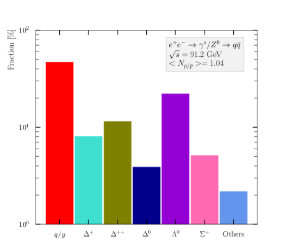
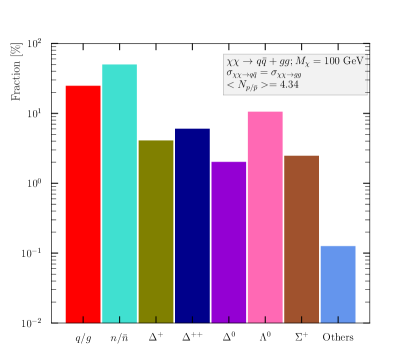
Figure 1: The mean contribution to $p/\bar{p}$ production in $e^{+}e^{-}\to\gamma^{*}/Z^{0}\to q\bar{q}$ at $\sqrt{s}=91.2~{}{\rm GeV}$ (left) and in dark matter annihilation into $q\bar{q}$ for $M_{\chi}=100~{}{\rm GeV}$ (right). Here, one shows $p/\bar{p}$ produced from QCD fragmentation, neutron decay, $\Delta^{+}$, $\Delta^{++}$, $\Delta^{0}$, $\Lambda^{0}$, $\Sigma^{+}$ and from other baryons.

In figure 1, we show the origin of protons in both $e^{+}e^{-}\to q\bar{q}$ at LEP (left) and in dark matter annihilation into $q\bar{q}$ for $M_{\chi}=100~{}{\rm GeV}$ (right). In general, (anti-)protons can be split into two categories: (i) primary (anti-)protons produced directly from the string fragmentation of quarks and gluons and (ii) secondary (anti-)protons produced from the decay of heavier baryons.

2.2 Experimental constraints

From the discussion in the previous subsection, it is clear that the modeling of antiprotons will be improved if one includes all the relevant measurements of proton spectra performed at LEP. Besides the measurements of the proton spectrum itself, one may expect some improvements from measurements of the spectra of the $\Lambda^{0}$ baryons as well. The $\Lambda^{0}$ baryons are dominant sources of secondary protons at LEP (about $22\%$). There is a strong correlation between the spectra of (anti-)protons and of $\Lambda^{0}$ baryons since all the $\Lambda^{0}$ baryons are reconstructed from their decays into $\pi p$. We do not expect significant improvements from measurements of other baryons such as $\Delta^{++}$ or $\Sigma^{\pm}$ as due to the limited precision on their differential rates. Therefore, the main constraining observables in this study will consist of a set of measurements of $\Lambda$ and $p/\bar{p}$ energy–momentum distributions. To guarantee a good agreement with the results of the previous study [44] (including an acceptable modelling of overall event properties), we also include measurements of meson spectra, event shapes and particle multiplicities. We have considered eight constraining measurements of proton and $\Lambda^{0}$ reported on by Aleph [55, 56], Delphi [57, 58, 59] and Opal [60, 61].

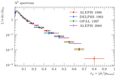
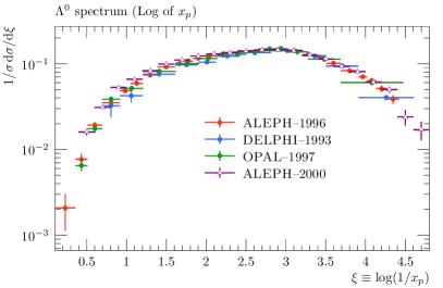
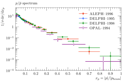
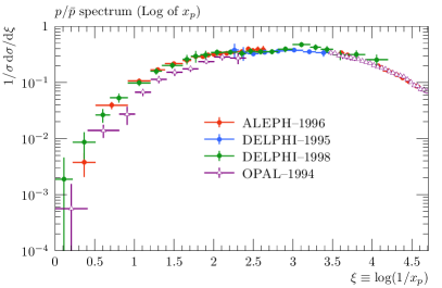
Figure 2: Comparison between the different measurements of the $\Lambda^{0}$ scaled momentum (upper panels) and of the proton scaled momentum (lower panels). Data is taken from [57, 55, 60, 58, 59, 62, 56, 63].

In figure 2, we show the comparisons between the different experimental measurements of $\Lambda^{0}$ spectrum and $p/\bar{p}$ spectrum. We can see that there are some inconsistencies between the measurement of the scaled momentum of $p/\bar{p}$ performed by Opal and the other experiments for $x_{p}>0.1$ (the Opal result is below all the others). Furthermore, the old Delphi measurement (blue) of $p/\bar{p}$ momentum is inconsistent with the new one (green) for few bins of $\xi\simeq 3$–$3.2$. Note that both these Delphi measurements cover the hole left by Aleph–1996. Finally, the Delphi–1993 measurement of $\Lambda^{0}$ scaled momentum seems to be inconsistent with the others for for $\xi<1.1$ (the discrepancy is mild as compared to the proton case). We do not include Opal–1994 measurement as it is inconsistent with all the other measurements for $x_{p}>0.1$ and Delphi–1995 as it was superseded by Delphi–1998 one.

3 Tunes of the fragmentation function

3.1 Phenomenological setup

This study aims to perform further retunings of the fragmentation function using Pythia8 version 8.244 [39] assuming the Monash tune [49] as our baseline. The different measurements used in our tunings are implemented in the validation package Rivet version 3.1.3 [51]. Both Frequentist and Bayesian tunings are performed using the optimisation tool Professor version 2.3.3 [50] and MultiNest [64]. Analytical expressions for the physical dependence of the observables on the different parameters are derived by fitting the Monte Carlo predictions to a set of points in the parameter space. In this study we assume a fourth-order polynomial interpolation to represent the true response of Pythia 8, i.e.

$$f_{(b)}(\{p_{i}\})=\alpha_{0}^{(b)}+\sum_{i=1}^{4}\beta_{i}^{(b)}p_{i}+\sum_{i,j=1}^{4}\gamma_{ij}^{(b)}p_{i}p_{j}+\sum_{i,j,k=1}^{4}\delta_{ijk}^{(b)}p_{i}p_{j}p_{k}+\sum_{i,j,k,\ell=1}^{4}\epsilon_{ijk\ell}^{(b)}p_{i}p_{j}p_{k}p_{\ell},$$ (3)

with $\alpha,\beta,\gamma,\delta,~{}{\rm and}~{}\epsilon$ are the polynomial coefficients determined in the fit and $\{p_{i}\}=\{a,\langle z_{\rho}\rangle,\sigma_{\perp},a_{\rm Diquark}\}$ are the parameters of the Lund fragmentation function (defined in table 1). The best-fit points for the parameters are determined by a standard $\chi^{2}$-minimisation method (Minuit [65]) implemented in Professor and which uses the analytical polynomial interpolations defined in equation 3.

The goodness-of-fit per number of degrees of freedom is defined as

$$\chi^{2}=\frac{1}{\sum_{\mathcal{O}}\omega_{\mathcal{O}}|b\in\mathcal{O}|-N_{\rm parameters}}\sum_{\mathcal{O}}\omega_{\mathcal{O}}\sum_{b\in\mathcal{O}}\bigg{(}\frac{f_{(b)}(\{p_{i}\})-\mathcal{R}_{b}}{\Delta_{b}}\bigg{)}^{2},$$ (4)

where $\mathcal{R}_{b}$ is the central value for the experimental measurement $\mathcal{O}$ at a bin $b$, $f_{(b)}(\{p_{i}\})$ is the analytical expression of the response function which is a polynomial of the parameters, and $\Delta_{b}$ is the total error which is quadratic sum of the statistical MC errors, the experimental errors and a flat $5\%$ theory errors:

$$\Delta_{b}=\sqrt{\sigma_{b,\rm exp}^{2}+\sigma_{b,{\rm MC}}^{2}+\sigma_{b,{\rm th}}^{2}},$$ (5)

with $\sigma_{b,{\rm th}}=0.05\times f_{(b)}(\{p_{i}\})$.

3.2 Results

Tune	aLund	avgZLund	sigma	aExtraDiquark	bLund	$\chi^{2}/N_{\rm df}$
Aleph	$0.758\begin{subarray}{c}+0.074\\ -0.074\end{subarray}$	$0.541\begin{subarray}{c}+0.007\\ -0.007\end{subarray}$	$0.297\begin{subarray}{c}+0.005\\ -0.005\end{subarray}$	$1.218\begin{subarray}{c}+0.358\\ -0.358\end{subarray}$	$1.040$	$116.22/296$
Delphi	$0.358_{-0.054}^{+0.054}$	$0.497_{-0.007}^{+0.007}$	$0.287_{-0.006}^{+0.006}$	$0.782_{-0.298}^{+0.298}$	$0.533$	$144.37/268$
L3	$0.478_{-0.063}^{+0.063}$	$0.557_{-0.006}^{+0.006}$	$0.315_{-0.007}^{+0.007}$	$1.998_{-0.049}^{+0.049}$	$0.897$	$84.70/140$
Opal	$0.588_{-0.086}^{+0.086}$	$0.536_{-0.005}^{+0.005}$	$0.300_{-0.005}^{+0.005}$	$1.998_{-0.204}^{+0.204}$	$0.872$	$53.54/136$
Combined	$0.601_{-0.038}^{+0.038}$	$0.540_{-0.004}^{+0.004}$	$0.307_{-0.002}^{+0.002}$	$1.671_{-0.196}^{+0.196}$	$0.897$	$676.69/852$

Table 2: Results of the tunes performed separately to all the considered measurements from a given experiment.

The results of the fragmentation function tunes are shown in table 2 for individual experiments and their combinations. We can see that the best-fit points of StringZ:aLund, StringZ:avgZLund and StringPT:sigma are consistent with the results of a previous study [44]. On the other hand, the best-fit point of StringZ:aExtraDiquark is larger than what we found in the one-dimensional parameter space tune. Note that this value is driven by the results from two experiments: L3 and Opal. In figure 3 we show one- and two-dimensional marginalized posterior distributions for the unimodular four-dimensional parameter space fit along with the $68\%$ and $95\%$ Bayesian credible intervals. We have also checked that these results do not correspond to flat directions as the best-fit point of StringZ:aExtraDiquark does not depend on the maximum value allowed in the scan. We finally note that the these tune results give fairly good agreement with data and the results are competitive with the baseline Monash tune.

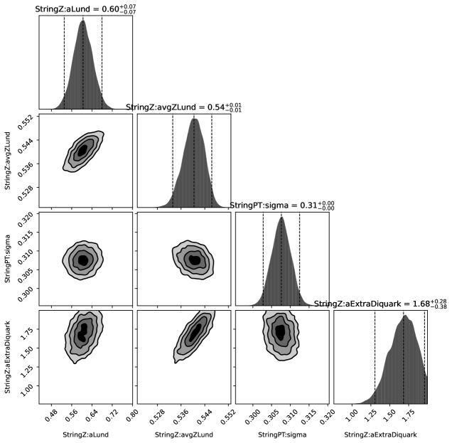
Figure 3: One- and two-dimensional marginalized posterior distributions for the uni-modal four-dimensional parameter space fit. Here, the contours show the $68\%$ and $95\%$ Bayesian credible intervals.

4 QCD uncertainties on antiproton spectra

4.1 Perturbative uncertainties

The perturbative uncertainties are split into catergories: scale variation uncertainties and non-singular (hard terms) uncertainties. The first class of the shower uncertainties are estimated by varying the renormalisation scale by a factor of two in each direction with respect to the nominal scale choice. To guarantee that scale variations are as conservative as possible, a number of modifications on the naive scale variations are done by adding some NLO compensation terms to absorb large corrections [66]. The variations of the non-universal hard components of the DGLAP kernels are also possible with the new automated formalism. We close this discussion by noting that Matrix-Element Corrections (MECs), switched on by default in Pythia 8, lead to very small variations of the non-singular terms of the DGLAP splittings for $Z^{0}$ decays. It was found that switching off these corrections would lead to comprehensively larger envelopes [66].

4.2 Fragmentation function uncertainties

Tune StringZ:aLund StringZ:avgZLund StringPT:sigma StringZ:aExtraDiquark Central $0.601$ $0.540$ $0.307$ $1.671$ $2\sigma$ eigentunes Variation $1^{+}$ $0.609$ $0.542$ $0.307$ $1.775$ Variation $1^{-}$ $0.591$ $0.538$ $0.307$ $1.558$ Variation $2^{+}$ $0.501$ $0.535$ $0.306$ $1.679$ Variation $2^{-}$ $0.700$ $0.544$ $0.308$ $1.662$ Variation $3^{+}$ $0.597$ $0.609$ $0.333$ $1.670$ Variation $3^{-}$ $0.603$ $0.474$ $0.283$ $1.671$ Variation $4^{+}$ $0.601$ $0.478$ $0.475$ $1.672$ Variation $4^{-}$ $0.600$ $0.581$ $0.197$ $1.669$

Table 3: The Hessian variations (eigentunes) for the nominal tune including all the measurements performed by Aleph. The variations correspond to $\Delta\chi^{2}=4$ ($95\%$ CL) with $\Delta\chi^{2}$ is defined as $\Delta\chi^{2}\equiv\chi^{2}_{\rm var}-\chi^{2}_{\rm min}$.

The Professor toolkit provides an estimate of the uncertainties on the fitted parameters through the Hessian method (also known as eigentunes). This method consists of a diagonalisation of the $\chi^{2}$ covariance matrix near the minimum which results in building a set of $2\cdot N_{\rm params}$ variations. These variations are then obtained as corresponding to a fixed change in the goodness-of-fit measure which is found by imposing a constraint on the maximum variation, defined as a hypersphere with maximum radius of $T$ (defined as the tolerance), i.e. $\Delta\chi^{2}\leq T$. Therefore one can define the $\Delta\chi^{2}$ to match a corresponding confidence level interval; i.e. one-sigma variations are obtained by requiring that $\Delta\chi^{2}\simeq N_{\rm df}$ where $N_{\rm df}$ is the number of degrees-of-freedom. This approach allows for a conservative estimate of the uncertainty if the event generator being used has a good agreement with data (which is usually quantified by $\chi^{2}_{\rm min}/N_{\rm df}\leq 1$) and the resulting uncertainties provide a good coverage of the errors in the experimental data. To enable for this situation, we have added an extra $5\%$ uncertainty to the MC predictions for all the observables and bins which already implied a $\chi^{2}/N_{\rm df}\leq 1$ in our fits as depicted in table 2. On the other hand, we enable for large uncertainties by considering not only the one-sigma eigentunes but also the two-sigma eigentunes (correspond to $\Delta\chi^{2}/N_{\rm df}=4$) and the three-sigma eigentunes (correspond to $\Delta\chi^{2}/N_{\rm df}=9$). The three-sigma eigentunes provide a very good coverage of all the experimental uncertianties in the data for meson and baryon spectra but results in unreasonably large uncertainties that overshot the experimental errors for e.g. event shapes or jet rates. The variations corresponding to the two-sigma eigentunes are shown in table 3.

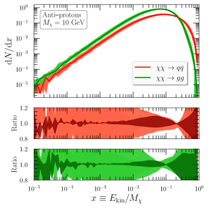
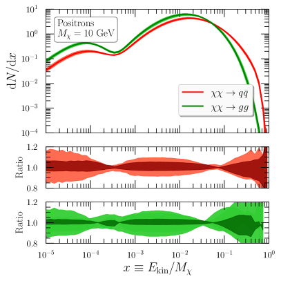
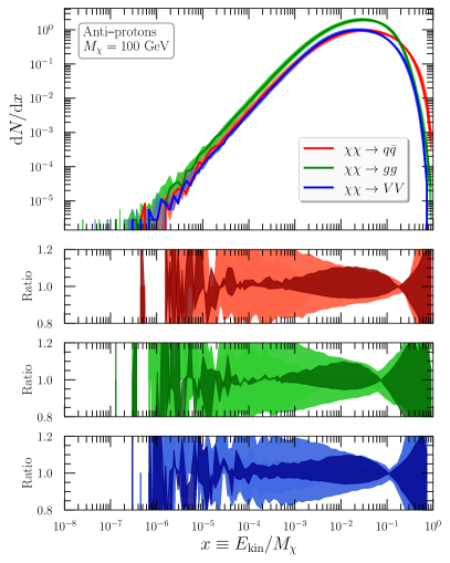
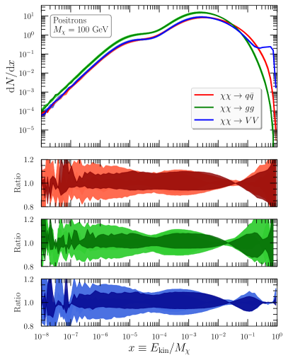
Figure 4: The scaled kinetic energy distribution of antiprotons (left) and positrons (right) in dark matter annihilation into $q\bar{q}$ (red), $gg$ (green) and $VV$ for dark matter mass of $10$ GeV (upper pane) and $100$ GeV (lower pane). For each pane, the dark shaded band corresponds to the parton-shower uncertainties while the light shaded band corresponds to hadronisation uncertainties.

4.3 Assessing QCD uncertainties on antiproton spectra

In this section, we quantify the impact of QCD uncertainties on particle spectra from dark matter annihilation for a few dark matter masses and annihilation channels. The results will be shown in the $x$ variable defined by

$$x\equiv\frac{E_{\rm kin}}{M_{\chi}}=\frac{E-m}{M_{\chi}},$$ (6)

with $E_{\rm kin}$ is the kinetic energy of the particle specie, $m$ is its mass and $M_{\chi}$ is the dark matter mass. We study the following annihilation channels:

$M_{\chi}$	$\chi\chi\to XX$	Spectra
$10~{}{\rm GeV}$	$q\bar{q}$, $gg$	Figure 4
$100~{}{\rm GeV}$	$q\bar{q}$, $gg$, $VV$	Figure 4

For the $q\bar{q}$ annihilation channel, we assume that the dark matter is annihilated to all the quarks except the top quark with ${\rm BR}(\chi\chi\to q\bar{q})=0.2,q=u,d,s,c,b$. For the $VV$ channel, we include both the $ZZ$ and $W^{+}W^{-}$ channels with equal probabilities: i.e. ${\rm BR}(\chi\chi\to W^{+}W^{-})={\rm BR}(\chi\chi\to ZZ)=0.5$. The impact of QCD uncertainties on the antiproton spectra are shown in figure 4. For comparison, we show the spectra of positrons as well. We can see that the QCD uncertainties resulting from parton-shower variations are subleading for dark matter mass of $10$ GeV and especially in the anti-matter spectra. As far as we go to high dark matter masses, for example $100$ GeV, these uncertainties become more competitive with the hadronisation uncertainties and reach up to $15\%$ in the peak region. The hadronisation uncertainties on the antiproton spectra are very important and can reach up to $20\%$ in the low energy region and about $10\%$ in the peak region. In the high energy region, both the perturbative and hadronisation uncertainties are important with the latter are dominant with respect to the former (and can reach up to $50\%$. Note that the position of the peak changes for some particle species. There are regions where all the variations result in no uncertainty at all, e.g. $x\simeq 0.2$ in the antiproton spectra in the $q\bar{q}$ final state.

5 Conclusions

In this talk, we discussed the study of the QCD uncertainties on antiproton spectra from DM annihilation which we studied for the first time in [44]. We first discussed the physics modeling of antiproton production from dark matter annihilation and the minimal set of constraining data. We then performed several retunings of the Lund fragmentation function parameters in Pythia 8. We provided a minimal set of variations on the parameters that define a conservative estimate of the QCD uncertainties allowed by data. We have finally shown quantitatively the impact of the QCD uncertainties on the spectra of antiprotons from DM annihilation into $q\bar{q}$, $gg$, and $WW+ZZ$. Full data tables which can be used to update those in the PPPC4DMID are public can be found on GitHub and can be found in https://github.com/ajueid/qcd-dm.github.io.git. The tables can also be found in the next releases of DarkSusy 6 [67] and MicrOmegas 5 [68].

References

- [1] R. L. Golden, S. Horan, B. G. Mauger, G. D. Badhwar, J. L. Lacy, S. A. Stephens, R. R. Daniel, and J. E. Zipse, EVIDENCE FOR THE EXISTENCE OF COSMIC RAY ANTI-PROTONS, Phys. Rev. Lett. 43 (1979) 1196–1199.
- [2] A. Buffington, S. M. Schindler, and C. R. Pennypacker, A measurement of the cosmic-ray antiproton flux and a search for antihelium, Astrophys. J. 248 (1981) 1179–1193.
- [3] J. Silk and M. Srednicki, Cosmic Ray anti-Protons as a Probe of a Photino Dominated Universe, Phys. Rev. Lett. 53 (1984) 624.
- [4] F. W. Stecker, S. Rudaz, and T. F. Walsh, Galactic Anti-protons From Photinos, Phys. Rev. Lett. 55 (1985) 2622–2625.
- [5] AMS Collaboration, M. Aguilar et al., Antiproton Flux, Antiproton-to-Proton Flux Ratio, and Properties of Elementary Particle Fluxes in Primary Cosmic Rays Measured with the Alpha Magnetic Spectrometer on the International Space Station, Phys. Rev. Lett. 117 (2016), no. 9 091103.
- [6] A. Cuoco, M. Krämer, and M. Korsmeier, Novel Dark Matter Constraints from Antiprotons in Light of AMS-02, Phys. Rev. Lett. 118 (2017), no. 19 191102, [arXiv:1610.03071].
- [7] M.-Y. Cui, Q. Yuan, Y.-L. S. Tsai, and Y.-Z. Fan, Possible dark matter annihilation signal in the AMS-02 antiproton data, Phys. Rev. Lett. 118 (2017), no. 19 191101, [arXiv:1610.03840].
- [8] A. Cuoco, J. Heisig, M. Korsmeier, and M. Krämer, Probing dark matter annihilation in the Galaxy with antiprotons and gamma rays, JCAP 10 (2017) 053, [arXiv:1704.08258].
- [9] A. Reinert and M. W. Winkler, A Precision Search for WIMPs with Charged Cosmic Rays, JCAP 01 (2018) 055, [arXiv:1712.00002].
- [10] M.-Y. Cui, X. Pan, Q. Yuan, Y.-Z. Fan, and H.-S. Zong, Revisit of cosmic ray antiprotons from dark matter annihilation with updated constraints on the background model from AMS-02 and collider data, JCAP 06 (2018) 024, [arXiv:1803.02163].
- [11] A. Cuoco, J. Heisig, L. Klamt, M. Korsmeier, and M. Krämer, Scrutinizing the evidence for dark matter in cosmic-ray antiprotons, Phys. Rev. D 99 (2019), no. 10 103014, [arXiv:1903.01472].
- [12] I. Cholis, T. Linden, and D. Hooper, A Robust Excess in the Cosmic-Ray Antiproton Spectrum: Implications for Annihilating Dark Matter, Phys. Rev. D 99 (2019), no. 10 103026, [arXiv:1903.02549].
- [13] S.-J. Lin, X.-J. Bi, and P.-F. Yin, Investigating the dark matter signal in the cosmic ray antiproton flux with the machine learning method, Phys. Rev. D 100 (2019), no. 10 103014, [arXiv:1903.09545].
- [14] M. Abdughani, Y.-Z. Fan, L. Feng, Y.-L. S. Tsai, L. Wu, and Q. Yuan, A common origin of muon g-2 anomaly, Galaxy Center GeV excess and AMS-02 anti-proton excess in the NMSSM, Sci. Bull. 66 (2021) 1545, [arXiv:2104.03274].
- [15] H. Hernandez-Arellano, M. Napsuciale, and S. Rodriguez, Cosmic-ray antiproton excess from annihilating tensor dark matter, arXiv:2108.10778.
- [16] T. Biekötter and M. O. Olea-Romacho, Reconciling Higgs physics and pseudo-Nambu-Goldstone dark matter in the S2HDM using a genetic algorithm, JHEP 10 (2021) 215, [arXiv:2108.10864].
- [17] L. Goodenough and D. Hooper, Possible Evidence For Dark Matter Annihilation In The Inner Milky Way From The Fermi Gamma Ray Space Telescope, arXiv:0910.2998.
- [18] Fermi/LAT Collaboration, Indirect Search for Dark Matter from the center of the Milky Way with the Fermi-Large Area Telescope, arXiv:0912.3828.
- [19] D. Hooper and L. Goodenough, Dark Matter Annihilation in The Galactic Center As Seen by the Fermi Gamma Ray Space Telescope, Phys. Rev. B697 (2011) 412–428, [arXiv:1010.2752].
- [20] C. Gordon and O. Macias, Dark Matter and Pulsar Model Constraints from Galactic Center Fermi-LAT Gamma Ray Observations, Phys. Rev. D88 (2013) 083521, [arXiv:1306.5725].
- [21] D. Hooper and T. Linden, On The Origin Of The Gamma Rays From The Galactic Center, Phys. Rev. D84 (2011) 123005, [arXiv:1110.0006].
- [22] T. Daylan, D. P. Finkbeiner, D. Hooper, T. Linden, S. K. N. Portillo, N. L. Rodd, and T. R. Slatyer, The characterization of the gamma-ray signal from the central Milky Way: A case for annihilating dark matter, Phys. Dark Univ. 12 (2016) 1–23, [arXiv:1402.6703].
- [23] B. Zhou, Y.-F. Liang, X. Huang, X. Li, Y.-Z. Fan, L. Feng, and J. Chang, GeV excess in the Milky Way: The role of diffuse galactic gamma-ray emission templates, Phys. Rev. D 91 (2015), no. 12 123010, [arXiv:1406.6948].
- [24] F. Calore, I. Cholis, and C. Weniger, Background model systematics for the Fermi GeV excess, JCAP 1503 (2015) 038, [arXiv:1409.0042].
- [25] K. N. Abazajian, N. Canac, S. Horiuchi, and M. Kaplinghat, Astrophysical and Dark Matter Interpretations of Extended Gamma-Ray Emission from the Galactic Center, Phys. Rev. D90 (2014), no. 2 023526, [arXiv:1402.4090].
- [26] A. Achterberg, S. Amoroso, S. Caron, L. Hendriks, R. Ruiz de Austri, and C. Weniger, A description of the Galactic Center excess in the Minimal Supersymmetric Standard Model, JCAP 1508 (2015), no. 08 006, [arXiv:1502.05703].
- [27] M. van Beekveld, W. Beenakker, S. Caron, and R. Ruiz de Austri, The case for 100 GeV bino dark matter: A dedicated LHC tri-lepton search, JHEP 04 (2016) 154, [arXiv:1602.00590].
- [28] A. Butter, S. Murgia, T. Plehn, and T. M. P. Tait, Saving the MSSM from the Galactic Center Excess, Phys. Rev. D 96 (2017), no. 3 035036, [arXiv:1612.07115].
- [29] C. Karwin, S. Murgia, T. M. P. Tait, T. A. Porter, and P. Tanedo, Dark Matter Interpretation of the Fermi-LAT Observation Toward the Galactic Center, Phys. Rev. D 95 (2017), no. 10 103005, [arXiv:1612.05687].
- [30] A. Achterberg, M. van Beekveld, S. Caron, G. A. Gómez-Vargas, L. Hendriks, and R. Ruiz de Austri, Implications of the Fermi-LAT Pass 8 Galactic Center excess on supersymmetric dark matter, JCAP 1712 (2017), no. 12 040, [arXiv:1709.10429].
- [31] M. di Mauro, F. Donato, A. Goudelis, and P. D. Serpico, New evaluation of the antiproton production cross section for cosmic ray studies, Phys. Rev. D 90 (2014), no. 8 085017, [arXiv:1408.0288]. [Erratum: Phys.Rev.D 98, 049901 (2018)].
- [32] R. Kappl and M. W. Winkler, The Cosmic Ray Antiproton Background for AMS-02, JCAP 09 (2014) 051, [arXiv:1408.0299].
- [33] M. Kachelriess, I. V. Moskalenko, and S. S. Ostapchenko, New calculation of antiproton production by cosmic ray protons and nuclei, Astrophys. J. 803 (2015), no. 2 54, [arXiv:1502.04158].
- [34] M. W. Winkler, Cosmic Ray Antiprotons at High Energies, JCAP 02 (2017) 048, [arXiv:1701.04866].
- [35] M. Korsmeier, F. Donato, and M. Di Mauro, Production cross sections of cosmic antiprotons in the light of new data from the NA61 and LHCb experiments, Phys. Rev. D 97 (2018), no. 10 103019, [arXiv:1802.03030].
- [36] J. Heisig, M. Korsmeier, and M. W. Winkler, Dark matter or correlated errors: Systematics of the AMS-02 antiproton excess, Phys. Rev. Res. 2 (2020), no. 4 043017, [arXiv:2005.04237].
- [37] X. Artru and G. Mennessier, String model and multiproduction, Nucl. Phys. B70 (1974) 93–115.
- [38] B. Andersson, G. Gustafson, G. Ingelman, and T. Sjostrand, Parton Fragmentation and String Dynamics, Phys. Rept. 97 (1983) 31–145.
- [39] T. Sjöstrand, S. Ask, J. R. Christiansen, R. Corke, N. Desai, P. Ilten, S. Mrenna, S. Prestel, C. O. Rasmussen, and P. Z. Skands, An Introduction to PYTHIA 8.2, Comput. Phys. Commun. 191 (2015) 159–177, [arXiv:1410.3012].
- [40] J. Bellm et al., Herwig 7.0/Herwig++ 3.0 release note, Eur. Phys. J. C76 (2016), no. 4 196, [arXiv:1512.01178].
- [41] T. Gleisberg, S. Hoeche, F. Krauss, M. Schonherr, S. Schumann, F. Siegert, and J. Winter, Event generation with SHERPA 1.1, JHEP 02 (2009) 007, [arXiv:0811.4622].
- [42] M. Cirelli, G. Corcella, A. Hektor, G. Hutsi, M. Kadastik, et al., PPPC 4 DM ID: A Poor Particle Physicist Cookbook for Dark Matter Indirect Detection, JCAP 1103 (2011) 051, [arXiv:1012.4515].
- [43] J. A. R. Cembranos, A. de la Cruz-Dombriz, V. Gammaldi, R. A. Lineros, and A. L. Maroto, Reliability of Monte Carlo event generators for gamma ray dark matter searches, JHEP 09 (2013) 077, [arXiv:1305.2124].
- [44] S. Amoroso, S. Caron, A. Jueid, R. Ruiz de Austri, and P. Skands, Estimating QCD uncertainties in Monte Carlo event generators for gamma-ray dark matter searches, JCAP 05 (2019) 007, [arXiv:1812.07424].
- [45] S. Amoroso, S. Caron, A. Jueid, R. Ruiz de Austri, and P. Skands, Particle spectra from dark matter annihilation: physics modelling and QCD uncertainties, PoS TOOLS2020 (2021) 028, [arXiv:2012.08901].
- [46] A. Jueid, Studying QCD modeling of uncertainties in particle spectra from dark-matter annihilation into jets, J. Phys. Conf. Ser. 2156 (2021), no. 1 012057, [arXiv:2110.09747].
- [47] A. Jueid, J. Kip, R. R. de Austri, and P. Skands, Impact of QCD uncertainties on antiproton spectra from dark-matter annihilation, arXiv:2202.11546.
- [48] A. Jueid, J. Kip, R. Ruiz de Austri Bazan, and P. Skands, The Strong Force meets the Dark Sector: A robust estimate of QCD uncertainties for anti-matter dark matter searches, in preparation.
- [49] P. Skands, S. Carrazza, and J. Rojo, Tuning PYTHIA 8.1: the Monash 2013 Tune, Eur. Phys. J. C74 (2014), no. 8 3024, [arXiv:1404.5630].
- [50] A. Buckley, H. Hoeth, H. Lacker, H. Schulz, and J. E. von Seggern, Systematic event generator tuning for the LHC, Eur. Phys. J. C65 (2010) 331–357, [arXiv:0907.2973].
- [51] C. Bierlich et al., Robust Independent Validation of Experiment and Theory: Rivet version 3, SciPost Phys. 8 (2020) 026, [arXiv:1912.05451].
- [52] P. Z. Skands, Tuning Monte Carlo Generators: The Perugia Tunes, Phys. Rev. D82 (2010) 074018, [arXiv:1005.3457].
- [53] T. Sjostrand, The Lund Monte Carlo for Jet Fragmentation, Comput. Phys. Commun. 27 (1982) 243.
- [54] T. Sjostrand, Jet Fragmentation of Nearby Partons, Nucl. Phys. B 248 (1984) 469–502.
- [55] ALEPH Collaboration, R. Barate et al., Studies of quantum chromodynamics with the ALEPH detector, Phys. Rept. 294 (1998) 1–165.
- [56] ALEPH Collaboration, R. Barate et al., Inclusive production of pi0, eta, eta-prime (958), K0(S) and lambda in two jet and three jet events from hadronic Z decays, Eur. Phys. J. C 16 (2000) 613.
- [57] DELPHI Collaboration, P. Abreu et al., Production of Lambda and Lambda anti-Lambda correlations in the hadronic decays of the Z0, Phys. Lett. B 318 (1993) 249–262.
- [58] DELPHI Collaboration, P. Abreu et al., Inclusive measurements of the K+- and p / anti-p production in hadronic Z0 decays, Nucl. Phys. B 444 (1995) 3–26.
- [59] DELPHI Collaboration, P. Abreu et al., pi+-, K+-, p and anti-p production in Z0 — q anti-q, Z0 — b anti-b, Z0 — u anti-u, d anti-d, s anti-s, Eur. Phys. J. C 5 (1998) 585–620.
- [60] OPAL Collaboration, R. Akers et al., Measurement of the production rates of charged hadrons in e+ e- annihilation at the Z0, Z. Phys. C63 (1994) 181–196.
- [61] OPAL Collaboration, G. Alexander et al., Strange baryon production in hadronic Z0 decays, Z. Phys. C73 (1997) 569–586.
- [62] SLD Collaboration, K. Abe et al., Production of pi+, K+, K0, K*0, phi, p and Lambda0 in hadronic Z0 decays, Phys. Rev. D59 (1999) 052001, [hep-ex/9805029].
- [63] SLD Collaboration, K. Abe et al., Production of pi+, pi-, K+, K-, p and anti-p in light (uds), c and b jets from Z0 decays, Phys. Rev. D69 (2004) 072003, [hep-ex/0310017].
- [64] F. Feroz, M. P. Hobson, and M. Bridges, MultiNest: an efficient and robust Bayesian inference tool for cosmology and particle physics, Mon. Not. Roy. Astron. Soc. 398 (2009) 1601–1614, [arXiv:0809.3437].
- [65] F. James and M. Roos, Minuit: A System for Function Minimization and Analysis of the Parameter Errors and Correlations, Comput. Phys. Commun. 10 (1975) 343–367.
- [66] S. Mrenna and P. Skands, Automated Parton-Shower Variations in Pythia 8, Phys. Rev. D94 (2016), no. 7 074005, [arXiv:1605.08352].
- [67] T. Bringmann, J. Edsjö, P. Gondolo, P. Ullio, and L. Bergström, DarkSUSY 6 : An Advanced Tool to Compute Dark Matter Properties Numerically, JCAP 07 (2018) 033, [arXiv:1802.03399].
- [68] G. Bélanger, F. Boudjema, A. Goudelis, A. Pukhov, and B. Zaldivar, micrOMEGAs5.0 : Freeze-in, Comput. Phys. Commun. 231 (2018) 173–186, [arXiv:1801.03509].