Numerical package for QFT calculations of defect-induced phenomena in graphene

Abstract

We introduce a computationally efficient method based on the path integral formalism to describe defect-modified graphene. By taking into account the entire Brillouin zone, our approach respects the lattice symmetry and can be used to investigate both short-range and long-range effects. The proposed method’s key advantage is that the computational complexity does not increase with the system size, scaling, instead, with the number of defects. As a demonstration of our method, we explore the graphene-mediated RKKY interaction between multiple magnetic impurities. Our results concur with earlier findings by showing that the interaction strength and sign depend on various factors like impurity separation, sublattice arrangement, and system doping. We demonstrate that frustration can be introduced between the impurity spins by controlling their relative positions and that this frustration can be switched on and off by tuning the chemical potential of the system.

I Introduction

Theoretical studies of defects in graphene typically take one of three approaches: DFT simulations for atomically-precise short-range features, [Yazyev2007, Boukhvalov2008, Gerber2010afs, Park2012msa, Park2013spe, Frank2017] exact diagonalization of the tight-binding Hamiltonian for large but finite systems, where retaining the lattice structure is essential, [Garcia-Lastra2010sdb, Black-Schaffer2010rci, Jung2013] and the computationally-efficient $\mathbf{k}\cdot\mathbf{p}$ Dirac Hamiltonian to describe long-range and low-energy phenomena. [Pereira2007, Shytov2007, Shytov2007a, Uchoa2008, CastroNeto2009, Shytov2009lri, Kogan2011rii, Lebohec2014art, Agarwal2017lre, Frank2017, Agarwal2019pas] Over the past decade, advances in graphene fabrication and manipulation have made the highly-controlled experimental investigation of atomic-scale phenomena possible. For example, atomically precise deposition of adsorbates has allowed researchers to explore the role of impurity interaction in magnetism [GonzalezHerrero2016asc], study electronic scattering due to individual impurities [Brar2011], and confirm the supercritical potential regime predicted theoretically [Wang2013, Lu2019]. Moreover, individual-atom doping [Telychko2014, Telychko2015] made it possible to observe the Berry phase in the presence of single nitrogen atoms [Dutreix2019], induce a controlled migration of silicon dopants [Tripathi2018ebm], and shed light on the effects of single dopants on the electronic structure of the host material. [Telychko2021a]

In a significant portion of experimental studies, highly localized perturbations give rise to spatially-extended features. Consequently, one may deem the exact diagonalization an ideal approach as DFT becomes computationally infeasible because of the large supercell requirements and the Dirac Hamiltonian fails to capture the appropriate structure close to the perturbation. There is, however, a caveat: the system used in the exact diagonalization calculations must be sufficiently large to avoid finite-size effects. Including multiple spatially separated defects increases the minimum system size as one needs to make sure that the system edges are far enough away from all the perturbations.

An approach that does not lead to a drastic increase in computational complexity with additional defects while also respecting the lattice symmetry involves the field-theoretic formulation of the problem using the full tight-binding Hamiltonian instead of the simplified $\mathbf{k}\cdot\mathbf{p}$ version. This method has been used to, for example, study the effects of individual hydrogen adsorbates [Noori2020, Noori2020a]. Unfortunately, despite the utility of this approach, it remains isolated from the experimental community for which it would be the most useful, partly because of the perceived difficulty of QFT. Moreover, even for the community members familiar with the formalism, the time and effort required to set up the computational pipeline using this approach are substantial because code from previous studies is either not readily available or not fit for use by outside parties. As a result, there is a lot of redundant effort in the community, slowing down the research progress.

In this work, we introduce GrapheneQFT.jl, [rodinalex_harshitra-m_2022] an extendable package written in JULIA programming language [Bezanson2017] designed to calculate a variety of experimentally relevant QFT quantities in graphene in the presence of external perturbations. In particular, this package can compute electronic density, Green’s and spectral functions, and free energy in a graphene system containing adsorbates, dopants, and local gating. The paper is organized in the following manner. In Sec. II, we introduce the model and derive the relevant expressions to be used in the calculations. This is an analytical section and the reader more interested in the applications of the package can move directly to Sec. III, where we demonstrate the use of the package. Specifically, we focus here on the interaction between spin impurities in graphene via the Ruderman-Kittel-Kasuya-Yoshida (RKKY) coupling. [PhysRev.96.99, 10.1143/PTP.16.45, PhysRev.106.893] We investigate the sign dependence of the RKKY interaction on the system parameters and the impurity arrangement.  [Saremi2007rih, Black-Schaffer2010rci, Agarwal2017lre] Summary and outlook are provided in Sec. LABEL:sec:Summary.

II Model

II.1 Two-Component System

Instead of starting directly with the problem of defects in graphene, we begin by focusing on a more general scenario which will make the derivation more transparent. Consider two quantum systems described by single-particle second-quantized Hamiltonians $\sum_{jk}c^{\dagger}_{j}H_{jk}c_{k}$ and $\sum_{jk}d^{\dagger}_{j}h_{jk}d_{k}$, where $j$ and $k$ label the single-particle states in the systems. We will refer to the first system as “bulk” to indicate that it contains a large number of states compared to the second one, which we will label the “impurity” system.

Next, we introduce a coupling between the two systems and a perturbation that modifies the matrix elements for the bulk, leading to

$$\hat{\mathcal{H}} =\sum_{jk}c^{\dagger}_{j}H_{jk}c_{k}+\sum_{jk}g^{\dagger}_{j}h_{jk}g_{k}$$

$$+\sum_{jk}\left(c^{\dagger}_{j}V_{jk}g_{k}+g^{\dagger}_{k}V_{jk}^{*}c_{j}\right)+\sum_{jk}c^{\dagger}_{j}\Delta_{jk}c_{k}$$

$$=\mathbf{c}^{\dagger}H\mathbf{c}+\mathbf{c}^{\dagger}\Delta\mathbf{c}+\left(\mathbf{c}^{\dagger}V\mathbf{g}+\mathbf{g}^{\dagger}V^{\dagger}\mathbf{c}\right)+\mathbf{g}^{\dagger}h\mathbf{g}\,.$$ (1)

The coupling is given by the first term of the second line, while the bulk perturbation is the second term in the second line. As the final step, we made the Hamiltonian more compact by writing the sums as products of coupling matrices and vectors of operators.

The normal-ordered Hamiltonian in Eq. (1) can be transcribed into the imaginary-time action

$$S =\sum_{n}\Big{[}\bar{\boldsymbol{\psi}}_{n}\overbrace{\left(-i\omega_{n}-\mu+H\right)}^{-G^{-1}_{i\omega_{n}+\mu}}\boldsymbol{\psi}_{n}+\bar{\boldsymbol{\psi}}_{n}\Delta\boldsymbol{\psi}_{n}$$

$$+\left(\bar{\boldsymbol{\psi}}_{n}V\boldsymbol{\phi}_{n}+\bar{\boldsymbol{\phi}}_{n}V^{\dagger}\boldsymbol{\psi}\right)+\bar{\boldsymbol{\phi}}_{n}\underbrace{\left(-i\omega_{n}-\mu+h\right)}_{-\Gamma_{i\omega_{n}+\mu}^{-1}}\boldsymbol{\phi}_{n}\Big{]}$$

$$=\sum_{n}\begin{pmatrix}\bar{\boldsymbol{\psi}}_{n}&\bar{\boldsymbol{\phi}}_{n}\end{pmatrix}\begin{pmatrix}-G_{i\omega_{n}+\mu}^{-1}+\Delta&V\\ V^{\dagger}&-\Gamma_{i\omega_{n}+\mu}^{-1}\end{pmatrix}\begin{pmatrix}\boldsymbol{\psi}_{n}\\ \boldsymbol{\phi}_{n}\end{pmatrix}\,,$$ (2)

where $\omega_{n}$ are the fermionic Matsubara frequencies, $\mu$ is the chemical potential, and $\boldsymbol{\phi}_{n}$ and $\boldsymbol{\psi}_{n}$ ($\bar{\boldsymbol{\phi}}_{n}$ and $\bar{\boldsymbol{\psi}}_{n}$) are vectors of Grassmann numbers corresponding to $\mathbf{g}$ and $\mathbf{c}$ ($\mathbf{g}^{\dagger}$ and $\mathbf{c}^{\dagger}$). We identify $G_{z}$ and $\Gamma_{z}$ as the Green’s functions for the two isolated and unperturbed systems. The matrix form of the action makes it straightforward to calculate the partition function by exponentiating $-S$ and integrating over all the Grassmann variables:

$$\mathcal{Z} =\prod_{n}\Bigg{|}\beta\underbrace{\begin{pmatrix}-G_{i\omega_{n}+\mu}^{-1}+\Delta&V\\ V^{\dagger}&-\Gamma_{i\omega_{n}+\mu}^{-1}\end{pmatrix}}_{-\mathbf{G}_{i\omega_{n}+\mu}^{-1}}\Bigg{|}\,,$$ (3)

where $\beta=1/(k_{B}T)$. The quantity $\mathbf{G}_{z}$ is the full Green’s function for the composite system, given explicitly by

$$\mathbf{G}_{z}=\begin{pmatrix}\mathcal{G}_{z}&\ \mathcal{G}_{z}V\Gamma_{z}\\ \Gamma_{z}V^{\dagger}\mathcal{G}_{z}&\Gamma_{z}+\Gamma_{z}V^{\dagger}\mathcal{G}_{z}V\Gamma_{z}\end{pmatrix}\,,$$ (4)

where

$$\mathcal{G}_{z} =\left(G_{z}^{-1}-\Delta-V\Gamma_{z}V^{\dagger}\right)^{-1}$$

$$=G_{z}+G_{z}\left(\Delta+V\Gamma_{z}V^{\dagger}\right)$$

$$\times\left[1-G_{z}\left(\Delta+V\Gamma_{z}V^{\dagger}\right)\right]^{-1}G_{z}\,,$$ (5)

is the full Green’s function of the bulk and the bottom right block in Eq. (4) corresponds to the full Green’s function of the impurity states including their coupling to the perturbed bulk system.

From Eq. (5), one sees that $\mathcal{G}_{z}$ is comprised of two parts: the pristine bulk system $G_{z}$ and the perturbation-induced correction term, which we denote $\delta\mathcal{G}_{z}$. The matrix elements of $\delta\mathcal{G}_{z}$ are

$$\delta\mathcal{G}^{jk}_{z} =\sum_{lm}G^{jl}_{z}\Bigg{\{}\left(\Delta+V\Gamma_{z}V^{\dagger}\right)$$

$$\times\left[1-G_{z}\left(\Delta+V\Gamma_{z}V^{\dagger}\right)\right]^{-1}\Bigg{\}}_{lm}G^{mk}_{z}\,,$$ (6)

where the sum over $l$ and $m$ includes all the states in the bulk system. This expression can be made considerably simpler by rewriting $\Delta+V\Gamma_{z}V^{\dagger}$ in a block-diagonal form by rearranging the order of the states, where one block contains all the perturbed bulk the states and the other one contains the remainder (resulting in a block of all zeros). One can see from this rearrangement that only the states that are perturbed need to be included in the $lm$ summation. Thus, Eq. (6) can equivalently be written as

$$\delta\mathcal{G}^{jk}_{z} =\sum_{lm\in\textrm{pert}}G^{jl}_{z}\left[\left(\tilde{\Delta}+\tilde{V}\Gamma_{z}\tilde{V}^{\dagger}\right)\right.$$

$$\times\left.\left[1-\tilde{G}_{z}\left(\tilde{\Delta}+\tilde{V}\Gamma_{z}\tilde{V}^{\dagger}\right)\right]^{-1}\right]_{lm}G^{mk}_{z}\,,$$ (7)

where the tilde indicates that only the elements corresponding to the perturbed states are retained, substantially reducing the computational complexity. Note that a particular state is included in both $\tilde{V}$ and $\tilde{\Delta}$ even if it is perturbed by only one of the terms. Following a similar line of reasoning for the impurities, we get

$$\Gamma_{z}^{\mathrm{Full}}=\Gamma_{z}+\Gamma_{z}\tilde{V}^{\dagger}\tilde{G}_{z}\left[1-\left(\tilde{\Delta}+\tilde{V}\Gamma_{z}\tilde{V}^{\dagger}\right)\tilde{G}_{z}\right]^{-1}\tilde{V}\Gamma_{z}\,.$$ (8)

The diagonal terms of $\mathbf{G}_{z}$ can be used to calculate the expected particle number from

$$\rho_{j}=\frac{1}{\beta}\sum_{\omega_{n}}\left[\mathbf{G}_{i\omega_{n}+\mu}\right]_{jj}$$ (9)

and to obtain the corresponding spectral function

$$\mathcal{A}_{j}(\omega)=-2\mathrm{Im}\left[\mathbf{G}_{\omega+i0}\right]_{jj}\,.$$ (10)

From Eq. (3), we can also write down the Helmholtz free energy $F=-\beta^{-1}\ln\mathcal{Z}$:

$$F =-\beta^{-1}\sum_{n}\ln\left|\beta\begin{pmatrix}-G_{i\omega_{n}+\mu}^{-1}+\Delta&V\\ V^{\dagger}&-\Gamma_{i\omega_{n}+\mu}^{-1}\end{pmatrix}\right|$$

$$=-\beta^{-1}\sum_{n}\ln\Bigg{|}\beta\begin{pmatrix}-G_{i\omega_{n}+\mu}^{-1}&0\\ 0&-\Gamma_{i\omega_{n}+\mu}^{-1}\end{pmatrix}$$

$$\times\left[1+\begin{pmatrix}-G_{i\omega_{n}+\mu}&0\\ 0&-\Gamma_{i\omega_{n}+\mu}\end{pmatrix}\begin{pmatrix}\Delta&V\\ V^{\dagger}&0\end{pmatrix}\right]\Bigg{|}\,.$$ (11)

Removing the part of $F$ corresponding to the free energy of the two isolated systems in the absence of any perturbation yields the defect- and coupling-induced modification to $F$

$$\delta F =-\beta^{-1}\sum_{n}\ln\left|\begin{pmatrix}1-G_{i\omega_{n}+\mu}\Delta&-G_{i\omega_{n}+\mu}V\\ -\Gamma_{i\omega_{n}+\mu}V^{\dagger}&1\end{pmatrix}\right|$$

$$=-\beta^{-1}\sum_{n}\ln\left|1-\tilde{G}_{i\omega_{n}+\mu}\left(\tilde{\Delta}+\tilde{V}\Gamma_{i\omega_{n}+\mu}\tilde{V}^{\dagger}\right)\right|\,.$$ (12)

Next, we will show how Eqs. (9)-(12) are used to efficiently calculate interaction energy and electronic density in graphene in the presence of defects and impurities.

II.2 Graphene Green’s Function

With the formalism established, we now simply need to obtain the relevant Green’s functions for the system of interest and plug them into the expressions above. Because the electronic properties of graphene are dominated by the carbon $\pi$ orbitals, the electronic states in a pristine system can be described by $|\mathbf{r},L\rangle\otimes|\sigma\rangle$, where $\mathbf{r}$ is the coordinate of the unit cell hosting the orbital, $L$ is the sublattice of the atom, and $\sigma$ is the spin of the electron. Naturally, the infinitely-large monolayer corresponds to the bulk component in the discussion above so that the $|\mathbf{r},L\rangle\otimes|\sigma\rangle$ basis refers to the operators $c_{k}$ in Eq. (1).

To calculate the matrix elements of the graphene Green’s function $G_{z}=(z-H)^{-1}$ in the position basis, given by $\langle\mathbf{r},L|\otimes\langle\sigma|(z-\hat{H})^{-1}|\mathbf{r}^{\prime},L^{\prime}\rangle\otimes|\sigma^{\prime}\rangle$, it is useful to Fourier-transform the real-space states to get

$$\frac{1}{N}\sum_{\mathbf{qq}^{\prime}}\langle\mathbf{q},L|\otimes\langle\sigma|e^{i\mathbf{q}\cdot\mathbf{r}}(z-\hat{H})^{-1}e^{-i\mathbf{q}^{\prime}\cdot\mathbf{r}^{\prime}}|\mathbf{q}^{\prime},L^{\prime}\rangle\otimes|\sigma^{\prime}\rangle\,,$$ (13)

where the $\mathbf{q}$ and $\mathbf{q}^{\prime}$ momentum sums run over the entire Brillouin zone and $N$ is the number of states in the system. Because the momentum-space Hamiltonian is diagonal in $\mathbf{q}$ and $\sigma$, we can write the matrix elements as

$$\frac{1}{N}\sum_{\mathbf{q}}\langle\mathbf{q},L|e^{i\mathbf{q}\cdot\mathbf{r}}(z-\hat{H})^{-1}e^{-i\mathbf{q}\cdot\mathbf{r}^{\prime}}|\mathbf{q},L^{\prime}\rangle\delta_{\sigma\sigma^{\prime}}$$

$$= \langle L|\frac{1}{N}\sum_{\mathbf{q}}e^{i\mathbf{q}\cdot\left(\mathbf{r}-\mathbf{r}^{\prime}\right)}(z-H_{\mathbf{q}})^{-1}|L^{\prime}\rangle\delta_{\sigma\sigma^{\prime}}\,.$$ (14)

The graphene tight-binding Hamiltonian with the nearest-neighbor hopping is given by

$$H_{\mathbf{q}}=\begin{pmatrix}0&-tf_{\mathbf{q}}\\ -tf^{*}_{\mathbf{q}}&0\end{pmatrix}\,,$$ (15)

where $t=2.8\,\textrm{eV}$ is the hopping integral, $f_{\mathbf{q}}=1+e^{i\mathbf{q}\cdot\mathbf{d}_{1}}+e^{i\mathbf{q}\cdot\mathbf{d}_{2}}$, and $\mathbf{d}_{1/2}=d\left(\pm 1,\sqrt{3}\right)/2$ are the lattice vectors. From Eq. (14), we have

$$\frac{1}{N}\sum_{\mathbf{q}}\left(z-H_{\mathbf{q}}\right)^{-1}e^{i\left(\mathbf{r}_{k}-\mathbf{r}_{j}\right)\cdot\mathbf{q}}$$

$$= \frac{1}{N}\sum_{\mathbf{q}}\begin{pmatrix}z&-tf_{\mathbf{q}}\\ -tf_{\mathbf{q}}^{*}&z\end{pmatrix}\frac{1}{z^{2}-t^{2}\left|f_{\mathbf{q}}\right|^{2}}e^{i\mathbf{r}_{kj}\cdot\mathbf{q}}\,,$$ (16)

where $\mathbf{r}_{jk}=\mathbf{r}_{j}-\mathbf{r}_{k}$. To perform the summation over $\mathbf{q}$, we first introduce

$$\Omega^{u,v}_{z}=\frac{1}{N}\sum_{\mathbf{q}\in\mathrm{BZ}}\frac{e^{i\mathbf{q}\cdot\left(u\mathbf{d}_{1}+v\mathbf{d}_{2}\right)}}{z^{2}-t^{2}\left|f_{\mathbf{q}}\right|^{2}}$$ (17)

with $u\mathbf{d}_{1}+v\mathbf{d}_{2}=\frac{d}{2}\left(u-v,\sqrt{3}\left(u+v\right)\right)$. Writing $\mathbf{q}\cdot\left(u\mathbf{d}_{1}+v\mathbf{d}_{2}\right)=\frac{d}{2}\left[\left(u-v\right)q_{x}+\sqrt{3}\left(u+v\right)q_{y}\right]$ and turning the momentum sum into an integral yields

$$\Omega^{u,v}_{z}=\oint\frac{dx}{2\pi}\oint\frac{dy}{2\pi}\frac{e^{i\left[\left(u-v\right)x+\left(u+v\right)y\right]}}{z^{2}-t^{2}\left(1+4\cos^{2}x+4\cos x\cos y\right)}\,.$$ (18)

Using

$$\oint d\theta\frac{e^{il\theta}}{W-\cos\theta}=2\pi\frac{\left(W-\sqrt{W-1}\sqrt{W+1}\right)^{|l|}}{\sqrt{W-1}\sqrt{W+1}}\,,$$ (19)

turns Eq. (18) into

$$\Omega^{u,v}_{z}=\oint\frac{dx}{2\pi}\frac{e^{i\left(u-v\right)x}}{\cos x}\frac{\left(W-\sqrt{W-1}\sqrt{W+1}\right)^{|u+v|}}{4t^{2}\sqrt{W-1}\sqrt{W+1}}\,,$$ (20)

where $W=(z^{2}-t^{2})/(4t^{2}\cos x)-\cos x$. Finally, for $\mathbf{r}=u\mathbf{d}_{1}+v\mathbf{d}_{2}$, we have

$$\frac{1}{N}\sum_{\mathbf{q}}\left(z-H_{\mathbf{q}}\right)^{-1}e^{i\mathbf{r}\cdot\mathbf{q}}$$

$$=\begin{pmatrix}z\Omega^{u,v}_{z}&-t\left[\Omega^{u,v}_{z}+\Omega^{u,v}_{+,z}\right]\\ -t\left[\Omega^{u,v}_{z}+\Omega^{u,v}_{-,z}\right]&z\Omega^{u,v}_{z}\end{pmatrix}\,,$$ (21)

where

$$\Omega^{u,v}_{\pm,z}=\oint\frac{dx}{2\pi}\,2e^{i\left(u-v\right)x}\frac{\left(W-\sqrt{W-1}\sqrt{W+1}\right)^{|u+v\pm 1|}}{4t^{2}\sqrt{W-1}\sqrt{W+1}}\,.$$ (22)

The one-dimensional integrals over $x$ can be computed efficiently using Gaussian quadratures.

Using the multiples of the basis vectors to describe the electronic states, the matrix elements $\langle u,v,L|\otimes\langle\sigma|(z-\hat{H})^{-1}|u^{\prime},v^{\prime},L^{\prime}\rangle\otimes|\sigma^{\prime}\rangle$ of the Green’s function become

$$\langle u,v,L|\otimes\langle\sigma|(z-\hat{H})^{-1}|u^{\prime},v^{\prime},L^{\prime}\rangle\otimes|\sigma^{\prime}\rangle=\langle L|\begin{pmatrix}z\Omega^{u-u^{\prime},v-v^{\prime}}_{z}&-t\left[\Omega^{u-u^{\prime},v-v^{\prime}}_{z}+\Omega^{u-u^{\prime},v-v^{\prime}}_{+,z}\right]\\ -t\left[\Omega^{u-u^{\prime},v-v^{\prime}}_{z}+\Omega^{u-u^{\prime},v-v^{\prime}}_{-,z}\right]&z\Omega^{u-u^{\prime},v-v^{\prime}}_{z}\end{pmatrix}|L^{\prime}\rangle\delta_{\sigma\sigma^{\prime}}$$ (23)

with $|L^{\prime}\rangle$ and $\langle L|$ picking out the appropriate element of the matrix depending on the sublattices of the two states.

II.3 Hopping and Spin Defects

The $\Delta$ matrix introduced in Sec. II.1 describes the modified coupling between the states in the bulk. In the case of graphene, it can be used to encode an on-site potential, a modified hopping term, and an interaction between graphene’s electrons and localized spin moments. In the first case, $\Delta$ acquires diagonal terms for both spins, while for the hopping modification, $\Delta$ gets identical off-diagonal terms for the two spins.

To encode the coupling between graphene electrons and localized spins, recall that the spin-spin interaction can be written as $\mathbf{s}_{i}\cdot J_{ik}\cdot\hat{\boldsymbol{\sigma}}_{\sigma\sigma^{\prime}}c_{k\sigma}^{\dagger}c_{k\sigma^{\prime}}$, where $\mathbf{s}_{i}$ is the $i^{th}$ localized spin moment and $J_{ik}$ is the coupling constant between the $i^{th}$ spin and $k^{th}$ electronic state. We write $\mathbf{S}_{ik}=\mathbf{s}_{i}\times J_{ik}$ as the effective coupling strength between the spin and the carbon atom into which we absorbed the interaction strength and the spin angular momentum so that it has the units of energy. Writing out this expression for graphene yields

$$\mathbf{S}_{jk}\cdot\hat{\boldsymbol{\sigma}}_{\sigma\sigma^{\prime}}c_{\sigma,\mathbf{R}_{j}}^{\dagger}c_{\sigma^{\prime},\mathbf{R}_{j}} =(S_{z})_{jk}\left(c_{\uparrow,\mathbf{R}_{j}}^{\dagger}c_{\uparrow,\mathbf{R}_{j}}-c_{\downarrow,\mathbf{R}_{j}}^{\dagger}c_{\downarrow,\mathbf{R}_{j}}\right)$$

$$+\Big{(}(S_{x})_{jk}-i(S_{y})_{jk}\Big{)}c_{\uparrow,\mathbf{R}_{j}}^{\dagger}c_{\downarrow,\mathbf{R}_{j}}$$

$$+\Big{(}(S_{x})_{jk}+i(S_{y})_{jk}\Big{)}c_{\downarrow,\mathbf{R}_{j}}^{\dagger}c_{\uparrow,\mathbf{R}_{j}}\,,$$ (24)

where all the $c$ operators belong to either A or B sublattice. One can see that $S_{z}$ plays the role of a spin-dependent on-site potential, entering $\Delta$ as a diagonal term and the planar components of the localized spin give the hopping between the two spin orbitals of a carbon atom.

Treating the hopping perturbation on the same footing as the interaction with the localized spins makes it possible to simultaneously treat different defect types following the procedure outlined in Sec. II.1.

III Results

With the details of the formalism outlined in Sec. II, we can now use GrapheneQFT.jl to explore various defect configurations in graphene. Assuming that the user has Julia installed on their system, the package is installed and imported in the usual manner:

⬇

using Pkg; Pkg.add(”GrapheneQFT”)

using GrapheneQFT

The key object from which all physical quantities are computed is a GrapheneSystem}. This object, containing the system’s chemical potential, temperature, and the $\Delta$ and $V$ matrices defined in Sec.~\refsec:Two_Component_System, can be initialized using mkGrapheneSystem(μ, T, defects)}, where \mintinlinejuliadefects is an array of defects in the system. The defects can be of one of three types: localized states (corresponding to the impurity subsystem in Sec. II), a localized spin state, or a hopping modification. Below, we demonstrate how one can study the effects of localized spins and refer the reader to the package documentation [rodinalex_harshitra-m_2022] for more examples dealing with other defect types.

III.1 Local Electronic Density

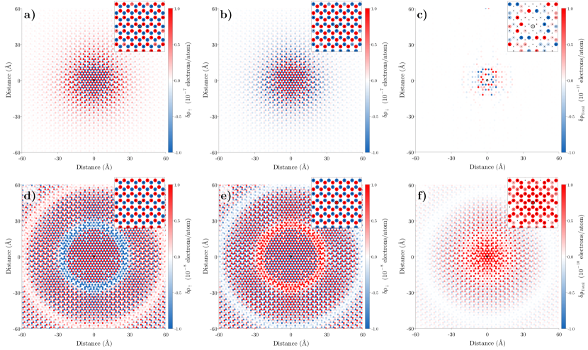
Figure 1: Spin-resolved and total electron density variation. From left to right: variation in spin-up, spin-down and total electron density for a system with a single magnetic impurity. The top row shows the variation at $\mu=0.0$ eV, while the bottom row shows the variation at $\mu=0.3$ eV. The impurity is located at the center of system (marked with black outline) with spin triplet $\mathbf{S}=J(0,0,1)$, where the spin-lattice coupling is set to $J=0.01$ eV. The inset plots show the electron density variation around the area close to impurity. Note that the color scale is saturated to demonstrate the sublattice dependence and the scale between the spin-resolved and total electron density varies greatly.

Consider a system with a single localized spin defect pointing in the $z$-direction, coupled to the A-sublattice atom at the unit cell with $u=v=0$. We first create a

GrapheneSystem} containing this spin:
%
\begin

minted[bgcolor = light-gray, breaklines]julia # System parameters μ = 0.0 T = 0.0 # Spin-lattice coupling J_val = 0.01 # Single spin defect single_spin_sys = mkGrapheneSystem(μ, T, Defect[LocalSpin(0.0, 0.0, J_val, GrapheneCoord(0, 0, A))]) The single entry in the Defect[]} array is the desired \mintinlinejuliaLocalSpin with $S_{x}=S_{y}=0$ and $S_{z}=J_{\mathrm{val}}$, coupled the graphene coordinate $(u=0,v=0,\mathrm{A})$. The function

mkGrapheneSystem} performs all the necessary manipulations to generate the required $\Delta$ and $V$ matrices.
Next, we calculate the defect-induced density. The local electronic density variation induced by the presence of defects, $\delta \rho_\mathbf

R$,canbecalculatedsimilarlytoEq.~{}\eqref{eqn:rho},exceptwiththediagonaltermsof$δG_iω_n + μ$.Thepackageprovidesafunction,makingthiscalculationstraightforward.Forexample,\text{δρ\_R\_graphene(GrapheneState(GrapheneCoord(4,5,B),Spin}$