Abstract

Unitary rotations of polychromatic images on finite two-dimensional pixellated screens provide invertibility, group composition, and thus conservation of information. Rotations have been applied on monochromatic image data sets, where we now examine closer the Gibbs-like oscillations that appear due to discrete ‘discontinuities’ of the input images under unitary transformations. Extended to three-color images we examine here the display of color at the pixels where, due to the oscillations, some pixel color values may fall outside their required common numerical range $[0,1]$, between absence and saturation of the red, green, and blue formant color images.

1 Introduction

In geometric and in wave optics, transformations that respect the Hamiltonian structure of the models are called canonical; they are termed linear when the phase space coordinates are linearly mapped. Images displayed on screens can undergo linear maps representing free propagation, rotation, gyration, squeezing, fractional Fourier and other transformations for one- or two-dimensional images on line or plane screens.

The discrete version of these systems and transformations, are based on the finite oscillator model [1, 2, 3], which considers finite pixellated line or plane screens that bear the set of generally complex data values that form the image. The requirement that the transformations be unitary to conserve Hilbert space properties of the image data sets (orthogonality, reality), requires them to be elements of a group, of which screen rotations form a one-parameter subgroup, to guarantee invertibility and proper concatenation for two or more such transformations. In particular, when the pixel values are real, they should remain so under rotation.

For this article to be essentially self-contained, in Sect. 2 we remind the reader of the basic finite oscillator model for $D=1$ and $D=2$-dimensional finite pixellated images along Cartesian coordinates [4]. We emphasize that this rotation algorithm provides the only unitary rotation coefficients for the image pixels on an $N_{x}\times N_{y}$ generally rectangular screen [5]. For simplicity we address here only square $N\times N$ images and screens.

In this paper we extend unitary rotations to polychromatic pixellated arrays that carry the three component color values (for red, green and blue) as generally used in the applied literature. In the polychromatic case, the ranges of the pixel values are restricted to the common interval $[0,1]$, between absence and saturation of each color. The main problem that appears now is that of Gibbs-like oscillations in one or more color component images of pixel values that may fall outside that basic $[0,1]$ range. This must be addressed with an appropriate display tactic, which is laid out in Sect. 3. Finally, in the concluding Sect. 4, we comment further on linear unitary transformations of pixellated data that are required to conserve information and Hamiltonian structure.

2 Finite one- and two-dimensional images

The finite oscillator model [6] is based on the Lie algebra of spin su($2$), with generators $\{J_{1},J_{2},J_{3}\}$ of commutation relations $[J_{i},J_{j}]=\varepsilon_{i,j,k}J_{k}$ ($i,j,k$ cyclic), whose representation multiplets, of dimension $N=2j+1$ (with $j$ a non-negative integer or half-integer), are interpreted to contain its $N$ equidistant eigenstates. The eigenvalues of the generator $Q:=J_{1}$ characterize the $N$ pixel positions on a screen, $P:=J_{2}$ is momentum, while those of $K:=J_{3}$ number the $N$ ‘energy’ states. The overlap between the position and mode eigenbases yields the finite oscillator wavefunctions. This finite model mimics the usual ‘continuous’ harmonic oscillator based on the Heisenberg-Weyl algebra (of commutator $[\overline{Q},\overline{P}]={\rm i}\hbar{\it 1}$, where the spectrum of position $\overline{Q}$ and of momentum $\overline{P}$ are the full real line), whose energy eigenstates of $\overline{H}:={\textstyle\frac{1}{2}}(\overline{P}^{2}+\overline{Q}^{2})$ are equally-spaced with only a lower bound.

2.1 The one-dimensional finite oscillator and screen

For $D=1$-dimensional screens of $N$ pixels in a line, the finite quantization of the harmonic oscillator replaces the commutator $[\overline{Q},\overline{P}]={\rm i}{\it 1}$ of the continuous model with $[Q,P]={\rm i}K$ in their $N=2j+1$-dimensional representation [1]. Finite quantization thus assigns $N\times N$ su($2$) matrix representations $\bf Q$ and $\bf P$ to position and momentum $q$ and $p$, as follows:

$${\hskip-15.0pt}\hbox{position}:\quad q\mapsto Q:=J_{1},\quad{\bf Q}=\|Q_{q,q^{\prime}}\|,$$ (1)

$$Q_{q,q^{\prime}}=q\,\delta_{q,q^{\prime}},\qquad q,q^{\prime}\in\{-j,-j{+}1,\ldots\,,j\},\quad N=:2j+1,$$

$${\hskip-15.0pt}\hbox{momentum}:\quad p\mapsto P:=J_{2},\quad{\bf P}=\|P_{q,q^{\prime}}\|,$$ (2)

$$P_{q,q^{\prime}}=-{\rm i}{\textstyle\frac{1}{2}}\sqrt{(j{-}q)(j{+}q{+}1)}\,\delta_{q+1,q^{\prime}}+{\rm i}{\textstyle\frac{1}{2}}\sqrt{(j{+}q)(j{-}q{+}1)}\,\delta_{q-1,q^{\prime}},$$

$${\hskip-15.0pt}\hbox{and their commutator}:\quad K:=J_{3},\quad{\bf K}=\|K_{q,q^{\prime}}\|,$$ (3)

$$K_{q,q^{\prime}}={\textstyle\frac{1}{2}}\sqrt{(j{-}q)(j{+}q{+}1)}\,\delta_{q+1,q^{\prime}}+{\textstyle\frac{1}{2}}\sqrt{(j{+}q)(j{-}q{+}1)}\,\delta_{q-1,q^{\prime}}.$$

These three operators are thus represented by self-adjoint $N\times N$ matrices in the vector space with inner product $\sum_{q=-j}^{j}f_{q}g_{q}^{*}$, and generate the Lie algebra su($2$) with commutation relations

$$[J_{i},J_{j}]={\rm i}\,\varepsilon_{i,j,k}J_{k},\quad\hbox{i.e.},\quad[K,Q]=-{\rm i}P,\ [K,P]={\rm i}Q,\ [Q,P]={\rm i}K,$$ (4)

where the first two will stand in place of the two Hamiltonian commutators in the continuous model, $[\overline{H},\overline{Q}]=-{\rm i}\overline{P}$ and $[\overline{H},\overline{P}]={\rm i}\overline{Q}$. The eigenvalue spectra of the three su($2$) generators are $\Sigma(Q)=\Sigma(P)=\Sigma(K)=\{-j,-j{+}1,\ldots\,,j\}=:|_{-j}^{j}$, and we remark that the position operator $Q=J_{1}$, is here diagonal. Finally, the eigenvalues of the mode operator $K+j{\it 1}$ will count its eigenstates by the mode number $n:=\kappa+j$ as

$$\ \Sigma(K+j{\it 1}):=\kappa+j=n\in\{0,\,1,\,\ldots,\,2j\}.$$ (5)

Using Dirac notation, let the orthogonal and complete eigenbases of the position and mode operators, $J_{1}$ and $J_{3}$, be

$$Q|j,q\rangle_{\scriptscriptstyle 1}=q|j,q\rangle_{\scriptscriptstyle 1},\ q|_{-j}^{j},\qquad K|j,n\rangle_{\scriptscriptstyle 3}=\kappa|j,n\rangle_{\scriptscriptstyle 3}=(n{-}j)|j,n\rangle_{\scriptscriptstyle 3},\ n|_{0}^{2j}.$$ (6)

One-dimensional finite signals or discrete images ${\bf F}=\{F_{q}\}_{q=-j}^{j}$ are then given by $N=(2j{+}1)$-dimensional vectors of components

$$F_{-j}={}_{\scriptscriptstyle 1}\langle j,-j|{\bf F}\rangle,\quad F_{-j+1}={}_{\scriptscriptstyle 1}\langle j,-j{+}1|{\bf F}\rangle,\quad\cdots\quad F_{j}={}_{\scriptscriptstyle 1}\langle j,j|{\bf F}\rangle.$$ (7)

The overlap between the two bases in (6) leads to a three-term difference equation that yields the Wigner ‘little-$d$’ functions [7] for the angle ${\textstyle\frac{1}{2}}\pi$ between the two axes, which are the finite oscillator wavefunctions [1]:

$$\begin{array}[]{rcl}\Psi_{n}(q)&:=&{}_{\scriptscriptstyle 1}\langle j,q|j,n\rangle_{\scriptscriptstyle 3}=d^{j}_{n-j,q}({\textstyle\frac{1}{2}}\pi)=\Psi_{q+j}(n{-}j)\\[7.0pt] &=&\displaystyle\frac{(-1)^{n}}{2^{j}}\sqrt{\bigg{(}{2j\atop n}\bigg{)}\bigg{(}{2j\atop q{+}j}\bigg{)}}\,K_{n}(q{+}j;{\textstyle\frac{1}{2}};2j),\end{array}$$ (8)

that are given in terms of the square root of a binomial coefficient in $q$, a discrete version of a Gaussian, and symmetric Kravchuk polynomials of degree $n$, $K_{n}(q{+}j;{\textstyle\frac{1}{2}};2j)=K_{q+j}(n;{\textstyle\frac{1}{2}};2j)={}_{2}F_{\!1}(-n,-2j{-}q;-2j;2)$, that are discrete analogues of Hermite polynomials. The set of functions $\{\Psi_{n}(q)\}_{n=0}^{2j}$, and also the set $\{\Psi_{n}(q)\}_{q=-j}^{j}$, form orthonormal bases for the $N$-dimensional space of signals (i.e., one-dimensional pixellated images on linear screens), so $\sum_{q=-j}^{j}\Psi_{n}(q)\Psi_{n^{\prime}}(q)=\delta_{n,n^{\prime}}$ and $\sum_{n=0}^{2j}\Psi_{n}(q)\Psi_{n}(q^{\prime})=\delta_{q,q^{\prime}}$.

Finally, we write the general form of the Wigner ‘little-$d$’ functions [7, Sect. 3.6],

$$\begin{array}[]{rcl}d^{j}_{m^{\prime},m}(\beta)&:=&d^{j}_{m,m^{\prime}}(-\beta)=\sqrt{(j+m^{\prime})(j-m^{\prime})(j+m)(j-m)}\\[5.0pt] &\times&\displaystyle\sum_{k}\frac{(-1)^{m^{\prime}-m+k}(\cos{\textstyle\frac{1}{2}}\beta)^{2j+m-m^{\prime}-2k}(\sin{\textstyle\frac{1}{2}}\beta)^{m^{\prime}-m+2k}}{k!\,(j+m-k)!\,(m^{\prime}-m+k)!\,(j-m^{\prime}-k)!},\end{array}$$ (9)

where the summation extends over the integer range $\hbox{max}(0,m{-}m^{\prime})\leq k\leq\hbox{min}(j{-}m)$ for $m>m^{\prime}$, while for $m<m^{\prime}$ the reflection formula in (8) applies.

2.2 Finite two-dimensional images

In $D=2$ dimensions, the finite oscillator Lie algebra is $\hbox{\sf su($2$)}_{x}\oplus\;\hbox{\sf su($2$)}_{y}=\hbox{\sf so($4$)}$, i.e., the four-dimensional orthogonal Lie algebra, which contains in particular the generator of an SO($2$) group of rotations in the $x$-$y$ plane. (Lie algebras are denoted by lower-case letters, their generated Lie groups by upper-case letters.) On a square screen, the so($4$) algebra represents finite images $\bf F$ by $N\times N$ matrices of entries $\{F_{q_{x},q_{y}}\}$, where $-j\leq q_{x},q_{y}\leq j$ are integer-spaced. Generic rectangular pixellated screens $N_{x}\times N_{y}$ have been considered in [5] with general representations of so($4$), but square ones are simpler and suffice for this study.

Finite 2D images can be characterized also by a second set of $N^{2}$ pixel values that follow polar coordinates responding to the subalgebra chain $\hbox{\sf so($4$)}\supset\hbox{\sf so($3$)}\supset\hbox{\sf so($2$)}$ [2]. The rotation of pixellated images in a square screen is then accomplished by transforming from the Cartesian to the polar basis, rotating through multiplicative phases in the polar basis, and transforming back to the Cartesian basis.

In two dimensions marked by orthogonal axes $x,\,y$, the algebra $\hbox{\sf su($2$)}_{x}\oplus\;\hbox{\sf su($2$)}_{y}$ provides two sets of generators (1)–(3) that mutually commute and provide, as in (6), their common eigenbases with $j_{x}=j=j_{y}$ (where we omit writing $j$ henceforth),

$$\begin{array}[]{ll}Q_{x}|q_{x},q_{y}\rangle_{\scriptscriptstyle 1}=q_{x}|q_{x},q_{y}\rangle_{\scriptscriptstyle 1},\ q_{x}|_{-j}^{j},&K_{x}|n_{x},n_{y}\rangle_{\scriptscriptstyle 3}=(n_{x}{-}j)|n_{x},n_{y}\rangle_{\scriptscriptstyle 3},\ n_{x}|_{0}^{2j},\\ Q_{y}|q_{x},q_{y}\rangle_{\scriptscriptstyle 1}=q_{y}|q_{x},q_{y}\rangle_{\scriptscriptstyle 1},\ q_{y}|_{-j}^{j},&K_{y}|n_{x},n_{y}\rangle_{\scriptscriptstyle 3}=(n_{y}{-}j)|n_{x},n_{y}\rangle_{\scriptscriptstyle 3},\ n_{y}|_{0}^{2j},\end{array}$$ (10)

defining the $N^{2}$ states $\{|q_{x},q_{y}\rangle_{\scriptscriptstyle 1}\}$ of the position basis and the $N^{2}$ states $\{|n_{x},n_{y}\rangle_{\scriptscriptstyle 3}\}$ of the mode basis. The overlap between these two orthogonal eigenbases provides the 2D finite Cartesian oscillator wavefunctions,

$$\Psi_{n_{x},n_{y}}(q_{x},q_{y})={}_{\scriptscriptstyle 1}\langle q_{x},q_{y}|n_{x},n_{y}\rangle_{\scriptscriptstyle 3}=\Psi_{n_{x}}(q_{x})\,\Psi_{n_{y}}(q_{y}).$$ (11)

As before, the set of functions $\{\Psi_{n_{x},n_{y}}(q_{x},q_{y})\}$ forms orthonormal bases for the $N^{2}$-dimensional space of pixellated two-dimensional images with respect to the indices $q_{x},q_{y}$ and with respect to $n_{x},n_{y}$.

Two-dimensional images ${\bf F}=\{F_{q_{x},q_{y}}\}_{q_{x},q_{y}=-j}^{j}$ are thus represented by the values of $N\times N$ matrices built with the adjoint of the position basis $|q_{x},q_{y}\rangle_{\scriptscriptstyle 1}$ in (10), as was done in (7) for one dimension,

$${\bf F}=\left(\begin{array}[]{ccc}{}_{\scriptscriptstyle 1}\langle-j,-j|&\cdots&{}_{\scriptscriptstyle 1}\langle-j,j|\\ \vdots&\ddots&\vdots\\ \phantom{-}{}_{\scriptscriptstyle 1}\langle j,-j|&\cdots&\phantom{-}{}_{\scriptscriptstyle 1}\langle j,j|\end{array}\right)\!|{\bf F}\rangle=\left(\begin{array}[]{ccc}F_{-j,-j}&\cdots&F_{-j,j}\\ \vdots&\ddots&\vdots\\ F_{j,-j}&\cdots&F_{j,j}\end{array}\right),$$ (12)

Next, according to the commutation relations (4), $K_{x}$ and $K_{y}$ generate independent rotations in the $(Q_{x},P_{x})$ and $(Q_{y},P_{y})$ phase planes. Their sum and difference have the eigenvalue sets

$$K:=K_{x}+K_{y}, \quad n:=n_{x}+n_{y}\in\{0,1,\ldots,4j\},$$ (13)

$$M:=K_{x}-K_{y}, \quad\!m:=n_{x}-n_{y}\in\{-2j,-2j{+}1,\ldots,2j\}.$$ (14)

There follows the definition of a distinct position-momentum basis [2] that is classified by the so($4$) generators

$$Q^{\circ}_{x}:=Q_{x}+Q_{y},\quad Q^{\circ}_{y}:=P_{x}-P_{y},\qquad P^{\circ}_{x}:=P_{x}+P_{y},\quad P^{\circ}_{y}:=-Q_{x}+Q_{y}.$$ (15)

With $K$ and $M$, these operators satisfy the commutation relations

$$\begin{array}[]{l}\Big{[}K,\,\Big{\{}{Q_{x}^{\circ}\atop P_{x}^{\circ}}\Big{]}={\rm i}\Big{\{}{\phantom{-}P_{x}^{\circ}\atop-Q_{x}^{\circ},}\quad\Big{[}K,\Big{\{}{Q_{y}^{\circ}\atop P_{y}^{\circ}}\Big{]}={\rm i}\Big{\{}{\phantom{-}P_{y}^{\circ}\atop-Q_{y}^{\circ},}\\[5.0pt] \Big{[}M,\Big{\{}{Q_{x}^{\circ}\atop Q_{y}^{\circ}}\Big{]}={\rm i}\Big{\{}{\phantom{-}Q_{y}^{\circ}\atop-Q_{x}^{\circ},}\quad\Big{[}M,\Big{\{}{P_{x}^{\circ}\atop P_{y}^{\circ}}\Big{]}={\rm i}\Big{\{}{\phantom{-}P_{y}^{\circ}\atop-P_{x}^{\circ},}\end{array}\qquad[K,M]=0,$$ (16)

that interpret $K$ as the generator of isotropic fractional Fourier-Kravchuk transforms [2, 3], and $M$ as the generator of rotations of the phase space operators in (15). The commuting operators $K,\,M$ define the orthonormal polar eigenbasis $\{|n,m\rangle_{\scriptscriptstyle P}\}$,

$$K|n,m\rangle_{\scriptscriptstyle P}=(n-2j)|n,m\rangle_{\scriptscriptstyle P},\ n|_{0}^{4j},\quad M|n,m\rangle_{\scriptscriptstyle P}=m|n,m\rangle_{\scriptscriptstyle P},\ m|_{-2j}^{2j}.$$ (17)

The overlap between the position basis and the polar basis determines the 2D finite polar oscillator wavefunctions [2],

$$\begin{array}[]{rcl}&&\Lambda^{j}_{n,m}(q_{x},q_{y}):={}_{\scriptscriptstyle 1}\langle q_{x},q_{y}|n,m\rangle_{\scriptscriptstyle P}\\[5.0pt] &&{\qquad}=\displaystyle(-1)^{(|m|-m)/2}\!\!\!\sum_{n_{x}+n_{y}=n}\!\!\!(-{\rm i})^{n_{y}}d^{n/2}_{\frac{1}{2}(n_{x}-n_{y}),\frac{1}{2}m}({\textstyle\frac{1}{2}}\pi)\,\Psi_{n_{x},n_{y}}(q_{x},q_{y}).\end{array}$$ (18)

Here also, the set of functions $\{\Lambda^{j}_{n,m}(q_{x},q_{y})\}$ provide orthonormal bases for the $N^{2}$-space of images, with respect to the indices $q_{x},q_{y}$ and with respect to $n,m$.

By construction, the functions (18) transform under rotations through multiplication by phases,

$${\cal R}(\theta)\Lambda^{j}_{n,m}(q_{x},q_{y}):=e^{-{\rm i}\theta M}\Lambda^{j}_{n,m}(q_{x},q_{y})=e^{-{\rm i}m\theta}\Lambda^{j}_{n,m}(q_{x},q_{y}),$$ (19)

The rotation of finite images ${\cal R}(\theta):|{\bf F}\rangle\mapsto|{\bf F}^{(\theta)}\rangle$ from the set $\{F_{q_{x},q_{y}}\}$ to $\{F_{\!q_{x},q_{y}}^{(\theta)}\}$ can thus proceed as

$$F_{\!q_{x},q_{y}}^{(\theta)} = {}_{\scriptscriptstyle 1}\langle q_{x},q_{y}|\,{\cal R}(\theta)\,|{\bf F}\rangle$$

$$= \!\!\!\!\sum_{n,m;q_{x}^{\prime},q_{y}^{\prime}}\!\!\!\!{}_{\scriptscriptstyle 1}\langle q_{x},q_{y}|n,m\rangle_{\scriptscriptstyle\!P}\,{}_{\scriptscriptstyle P\!}\langle n,m|{\cal R}(\theta)|n,m\rangle_{\scriptscriptstyle\!P}{}_{\scriptscriptstyle P\!}\langle n,m|q_{x}^{\prime},q_{y}^{\prime}\rangle_{\scriptscriptstyle 1}\,{}_{\scriptscriptstyle 1}\langle q_{x}^{\prime},q_{y}^{\prime}|{\bf F}\rangle$$

$$= \!\!\!\!\sum_{n,m;q_{x}^{\prime},q_{y}^{\prime}}\!\!\!\!{}_{\scriptscriptstyle 1}\langle q_{x},q_{y}|n,m\rangle_{\scriptscriptstyle\!P}\,e^{-{\rm i}m\theta}{}_{\scriptscriptstyle P\!}\langle n,m|q_{x}^{\prime},q_{y}^{\prime}\rangle_{\scriptscriptstyle 1}{}_{\scriptscriptstyle 1}\langle q_{x}^{\prime},q_{y}^{\prime}|{\bf F}\rangle{\qquad}$$

$$= \sum_{q_{x}^{\prime},q_{y}^{\prime}}R(q_{x},q_{y};q_{x}^{\prime},q_{y}^{\prime};\theta)\,F_{q^{\prime}_{x},q^{\prime}_{y}}$$ (21)

with $n|_{0}^{2j}$, $m|_{-2j}^{2j}$ and $q^{\prime}_{x},q^{\prime}_{y}|_{-j}^{j}$, where the kernel of rotation is given by

$$R(q_{x},q_{y};q_{x}^{\prime},q_{y}^{\prime};\theta):=\sum_{n,m}\Lambda^{j}_{n,m}(q_{x},q_{y})\,e^{-{\rm i}m\theta}\,\Lambda^{j}_{n,m}(q_{x}^{\prime},q_{y}^{\prime})^{*}.$$ (22)

An alternative expression for this kernel can be written as [2]

$$\begin{array}[]{l}\displaystyle R(q_{x},q_{y};q_{x}^{\prime},q_{y}^{\prime};\theta):=\sum_{\mu,\mu^{\prime}}\Psi_{n_{x},n_{y}}(q_{x},q_{y})\,d^{n/2}_{\mu,\mu^{\prime}}(2\theta)\,\Psi_{n_{x}^{\prime},n_{y}^{\prime}}(q_{x}^{\prime},q_{y}^{\prime})^{*},\\ \mu={\textstyle\frac{1}{2}}(n_{x}-n_{y}),\ \mu^{\prime}={\textstyle\frac{1}{2}}(n_{x}^{\prime}-n_{y}^{\prime});\quad n_{x}+n_{y}=n=n_{x}^{\prime}+n_{y}^{\prime}.\end{array}$$ (23)

When the input image is a matrix of real numbers, after rotation it will remain a real matrix, because the rotation kernel (22) is real. Due to the orthonormality of the bases, from (22) or (23), we see that $R(q_{x},q_{y};q_{x^{\prime}},q_{y^{\prime}};0)=\delta_{q_{x},q_{x^{\prime}}}\delta_{q_{y},q_{y^{\prime}}}$ is the unit transformation. Similarly, the product of two rotations satisfies group composition $\sum_{q_{x^{\prime}},q_{y^{\prime}}}R(q_{x},q_{y};q_{x^{\prime}},q_{y^{\prime}};\theta_{1})\*R(q_{x^{\prime}},q_{y^{\prime}};q_{x^{\prime\prime}},q_{y^{\prime\prime}};\theta_{2})=R(q_{x},q_{y};q_{x^{\prime\prime}},q_{y^{\prime\prime}};\theta_{1}+\theta_{2})$, and the inverse is $R(q_{x},q_{y};q_{x^{\prime}},q_{y^{\prime}};-\theta)=R(q_{x^{\prime}},q_{y^{\prime}};q_{x},q_{y};\theta)^{*}$. This shows that the matrices in the set (22) are unitary, ${\bf R}(-\theta)={\bf R}(\theta)^{\dagger}$, and is a representation of the group SO($2$) of plane rotations; it is reducible in the polar basis but irreducible in the Cartesian basis. As an example of this rotation algorithm we provide Fig. 1 that we proceed to examine and comment.

2.3 The ‘Gibbs-like’ oscillation phenomenon

As is evident in Fig. 1, a ubiquitous consequence of the unitarity of the rotation algorithm is that rotated images display oscillations due to ‘discrete discontinuities’, i.e., large differences between values of neighboring pixels. This oscillation pattern reminds us of that appearing in another context: the summation of truncated Fourier series, known as the Gibbs phenomenon. Because their origin is different (i.e., it is not a type of Gibbs oscillation), we shall call these oscillations Gibbs-like; here we address this phenomenon for the first time.

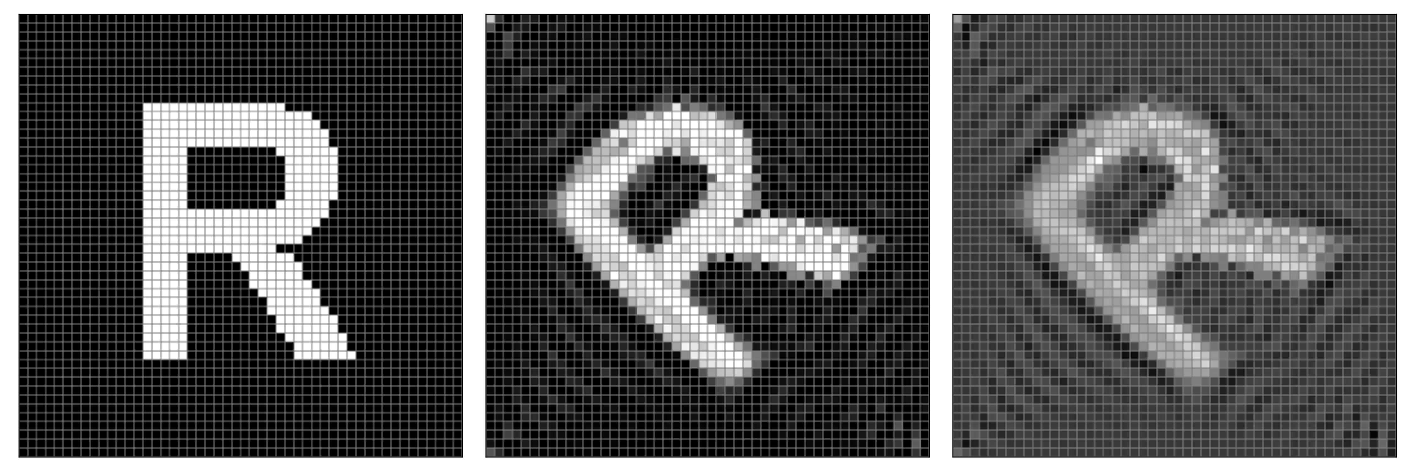
Figure 1: Left: A $50\times 50$ monochromatic image (letter “R”) of pixel values 1, over a background of pixel values 0. Center: Rotation of this image by $\frac{1}{4}\pi$ ($45^{\circ}$) with clipping of the over- and under-shoots beyond the obligate range $[0,1]$. Right: Same rotation with normalization of the pixel values to fit this range. Both output images exhibit ‘Gibbs-like’ oscillations due to the sharp boundaries of the input image. Whereas clipping leads to a more contrasted image, it also entails loss of information in pixel values; normalization retains information subject to translation and scale, although it appears less contrasted.

Linear normalization is the main tactic to keep the grey-tone scale within the specified range $[0,1]$, between absence and saturation of the pixel values. We thus distinguish between the data-image whose pixel values can have any range, and the screen-image which is output for display, where pixel values are all within $[0,1]$. This tactic maps the data- to screen-values, ${\bf F}\mapsto\overline{\bf F}$, using the extreme values,

$$F_{q_{x},q_{y}}\mapsto\overline{F}_{q_{x},q_{y}}=\frac{F_{q_{x},q_{y}}-s_{N}}{S_{N}-s_{N}},\quad\begin{array}[]{l}s_{N}\,:=\min_{q_{x},q_{y}}\,\{F_{q_{x},q_{y}}\}<0,\\ S_{N}:=\max_{q_{x},q_{y}}\,\{F_{q_{x},q_{y}}\}>1.\end{array}$$ (24)

The screen-image will thus have a minimum of complete blacks and whites, with no information loss.

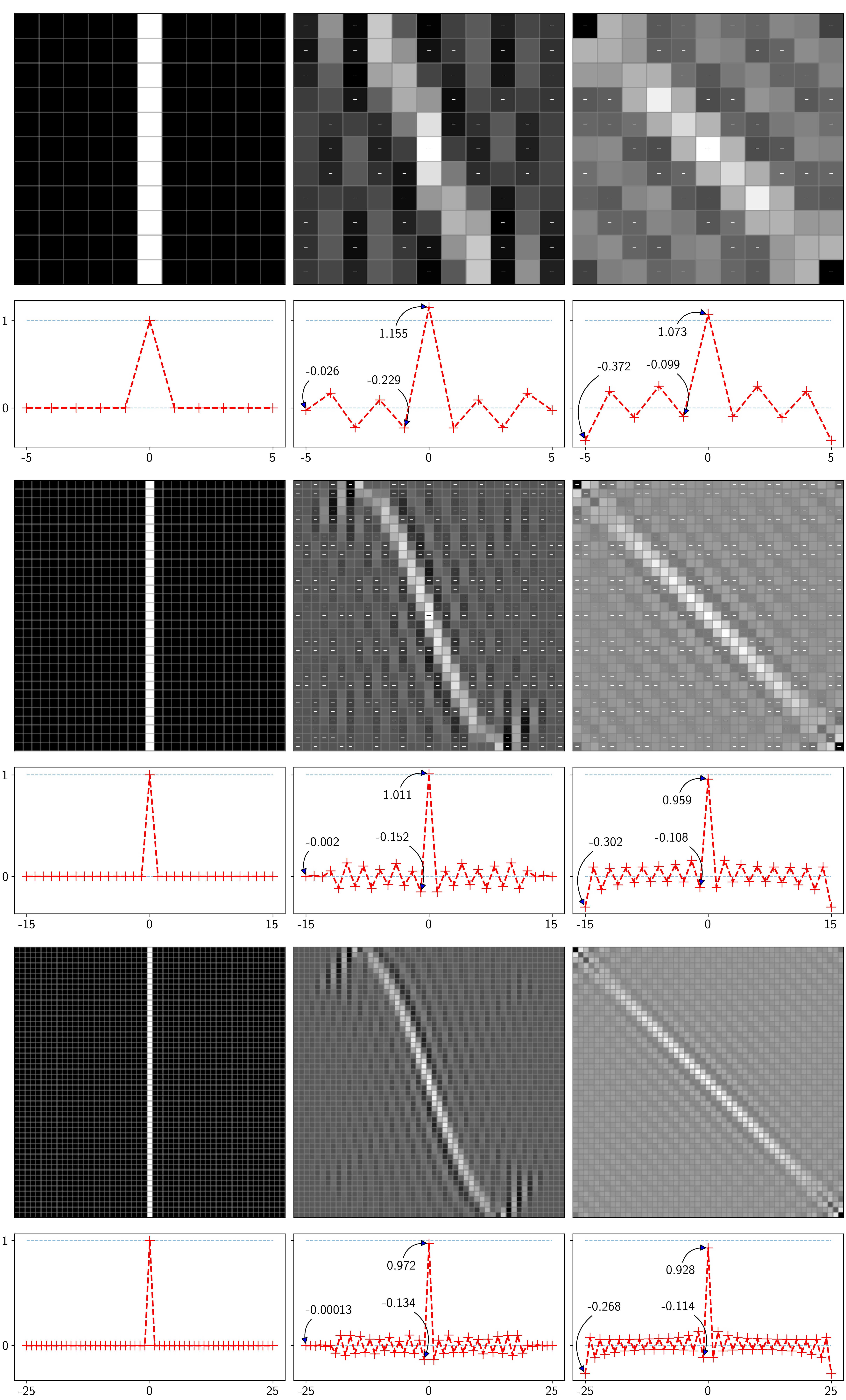
Figure 2: Unitary rotations of a centered Kronecker delta (25) for $N=11$, 31, 51, with their normalized rotated images. Left: the original discrete Kronecker function $\Delta^{{{\scriptscriptstyle(}}N)}_{{\scriptscriptstyle(}x{\scriptscriptstyle)}}(q_{x},q_{y})$ of 0 and 1. Center and Right: their images rotated by $\theta=\frac{1}{8}\pi$ and $\frac{1}{4}\pi$. Below each, the (non-normalized) values of anti-diagonal pixels, with their largest over- and undershoots. For $N=11$ and 31, the over- or under-shoots are marked by $+$ and $-$.

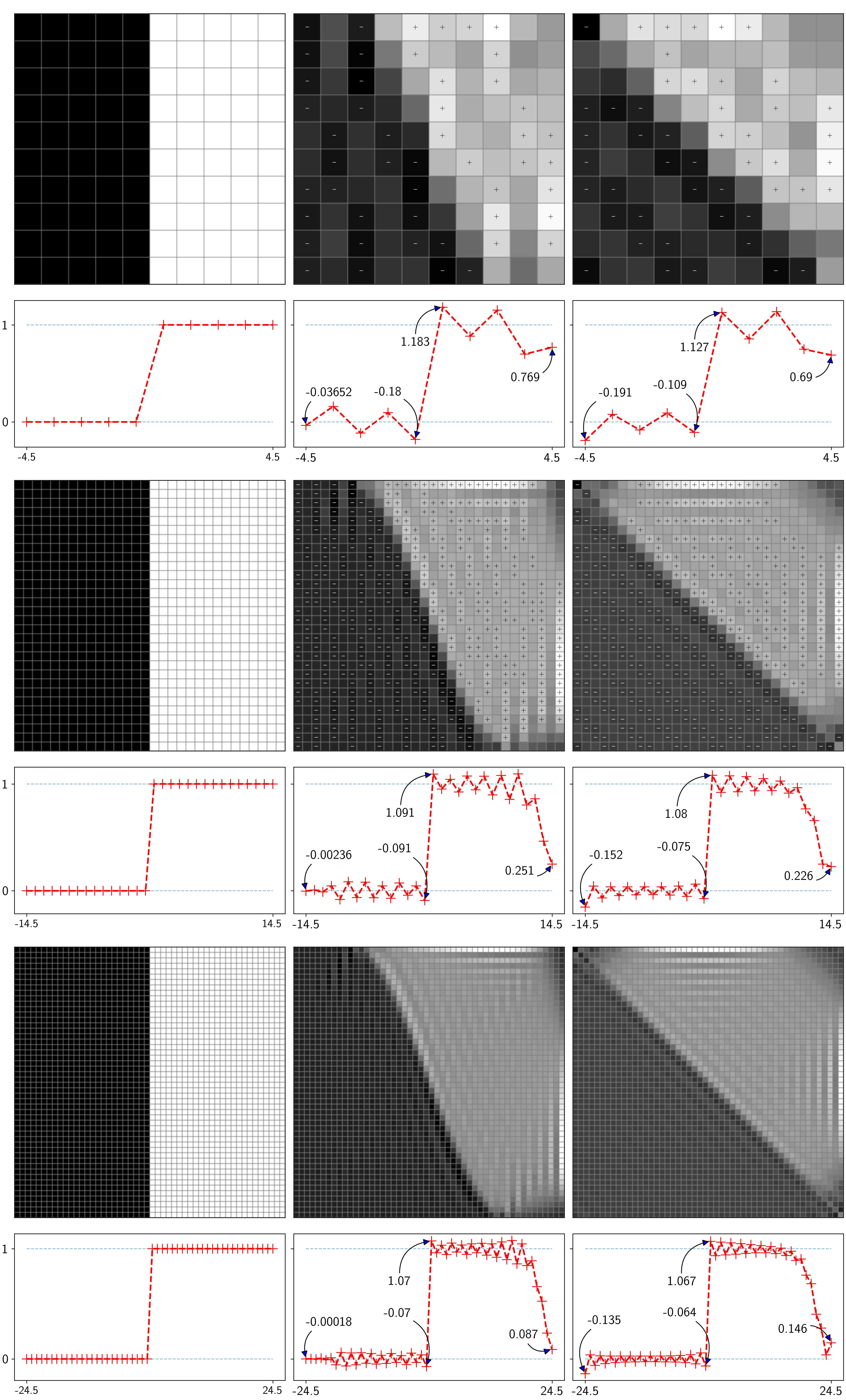
Figure 3: Unitary rotations of the unit step function (26) for $N=10$, 30, 50, with normalized rotated images, organized as in Fig. 2. Left: the step function $\Theta^{{{\scriptscriptstyle(}}N)}_{{\scriptscriptstyle(}x{\scriptscriptstyle)}}(q_{x},q_{y})$. Center and Right: rotatated images for $\theta=\frac{1}{8}\pi$ and $\frac{1}{4}\pi$.

Whereas in the familiar trigonometric Gibbs phenomenon, a unit step function $\Theta(q):={\textstyle\frac{1}{2}}(1+\hbox{sign}\,q)$ entails a maximal overshoot of ${\sim}8.95\%$ at a positions ever closer to the discontinuity as the number of series terms grows (see [9, Fig. 4.11 at p. 167]), to calibrate the Gibbs-like phenomenon for $N\times N$ images under unitary rotation, let us consider a Kronecker delta at the center of the screen with an odd number $N=2j+1$ of pixel rows and columns,

$$\Delta^{{{\scriptscriptstyle(}}N)}_{{\scriptscriptstyle(}x{\scriptscriptstyle)}}(q_{x},q_{y}):=\{0\hbox{ for }q_{y}<0,\ 1\hbox{ at }q_{y}=0,\ 0\hbox{ for }q_{y}>0\},$$ (25)

and a discrete step function along the $x$-axis for even $N=2j+1$ rows and columns

$$\Theta^{{{\scriptscriptstyle(}}N)}_{{\scriptscriptstyle(}x{\scriptscriptstyle)}}(q_{x},q_{y}):=\{0\hbox{ for }q_{y}\leq-{\textstyle\frac{1}{2}},\ 1\hbox{ for }q_{y}\geq{\textstyle\frac{1}{2}}\},$$ (26)

shown for rotations of $\frac{1}{8}\pi$ and $\frac{1}{4}\pi$ in Figs. 2 and 3 respectively. The resulting oscillations are recognizably parallel to the lines of discontinuity. To evince this oscillation behavior we plot below the pixel values along the main anti-diagonal of each screen

A first observation is that, unlike the continuous case, the over- and under-oscillations are not symmetrical. This is because while in the Gibbs case $e^{0{\rm i}x}=1$ belongs to the Fourier series terms and allows the addition of constants, in the discrete case $\Psi_{0,0}(q_{x},q_{y})$ is not a constant that could be freely added to all pixel values. Most importantly, we note that the over- and under-shoots diminish with increasing $N$: as the pixellation becomes finer, the finite oscillator states approximate those of continuous systems —as expected. Yet, although the delta and step functions lead to rotated images that are relatively simple to write analytically, they are not very useful to elucidate certain systematic features of their rotated images on the pixellated screen, such as the the behavior on and near the screen vertices and edges, as can be seen in those figures.

3 Three-color pixellated images

With a qualitative understanding of oscillations due to discrete Kronecker deltas and step functions, we now extend the algorithm from rotations of monochromatic finite $N\times N$ pixellated images presented in the previous section, to polychromatic images within the standard three-color scheme of RGB (Red-Green-Blue) technology. Each channel, R, G or B, is a monochromatic image; polychromatic images (indicated by sans serif font) are the direct sum of the three components where the pixel values for each color are all in the range $[0,1]$,

$${\sf F}={\bf F}^{\scriptscriptstyle\rm R}\oplus{\bf F}^{\scriptscriptstyle\rm G}\oplus{\bf F}^{\scriptscriptstyle\rm B},\quad{}_{\scriptscriptstyle 1\!}\langle q_{x},q_{y}|{{\sf F}}\rangle=\left[\begin{array}[]{l}\scriptstyle{}_{\scriptscriptstyle 1\!}\langle q_{x},q_{y}|{\bf F^{\scriptscriptstyle\rm R}}\rangle\\[-3.0pt] \scriptstyle{}_{\scriptscriptstyle 1\!}\langle q_{x},q_{y}|{\bf F^{\scriptscriptstyle\rm G}}\rangle\\[-3.0pt] \scriptstyle{}_{\scriptscriptstyle 1\!}\langle q_{x},q_{y}|{\bf F^{\scriptscriptstyle\rm B}}\rangle\end{array}\right]\!\!,\quad 0\leq{}_{\scriptscriptstyle 1\!}\langle q_{x},q_{y}|{\bf F^{\scriptscriptstyle\rm X}}\rangle\leq 1,$$ (27)

where X stands for R, G or B, with values 0 for absence and 1 for saturation in each color.

Under rotation we let each component undergo the same transformation (2.2)–(22) detailed in the previous section,

$${{\sf F}}^{(\theta)}:={\cal R}(\theta){{\sf F}}={\cal R}(\theta){\bf F}^{\scriptscriptstyle\rm R}\oplus{\cal R}(\theta){\bf F}^{\scriptscriptstyle\rm G}\oplus{\cal R}(\theta){\bf F}^{\scriptscriptstyle\rm B}.$$ (28)

The RGB color scheme is an industrial standard [14] that entails an additive colorimetric scale, that is, each of the elements of each channel sums to define an individual color [11, 12]. Physically, each of the colors in the RGB scheme is associated with the way the human eye perceives and processes light with the photoreceptor cells in the retina [13]. The chromatic response is intrinsic to the aggregation of the three channels and independent of the luminescence, which means that the white point of the scale is the algebraic sum of the three channel values, and independent of the illumination [21]. This color scheme is strictly positive within a range of bits or bytes displayed in digital or analogue devices [15, 16]. Although pixel values outside the standard range have been also used as representing complementary colors [18, 17], we forego this alternative interpretation because it would introduce dubious changes in the color rendering of black or white backgrounds.

Here we address the joint display of the three data-image matrices to acceptably transform color images. The normalization of pixel values (24) now requires the extreme values among the three colors to define, for $Y\in\{R,G,B\}$,

$$F_{q_{x},q_{y}}^{{\scriptscriptstyle\rm Y}}\mapsto\overline{F}_{q_{x},q_{y}}^{{\scriptscriptstyle\rm Y}}=\frac{F_{q_{x},q_{y}}^{{\scriptscriptstyle\rm Y}}-s_{N}}{S_{N}-s_{N}},\quad\begin{array}[]{l}s_{N}\,:=\min_{X;\,q_{x},q_{y}}\,\{F_{q_{x},q_{y}}^{{\scriptscriptstyle\rm X}}\}<0,\\ S_{N}:=\max_{X;\,q_{x},q_{y}}\,\{F_{q_{x},q_{y}}^{{\scriptscriptstyle\rm X}}\}>1.\end{array}$$ (29)

Two examples of this unitary rotation algorithm for three-color images are presented in Figs. 4, for images with high and low pixel discontinuity contrasts.

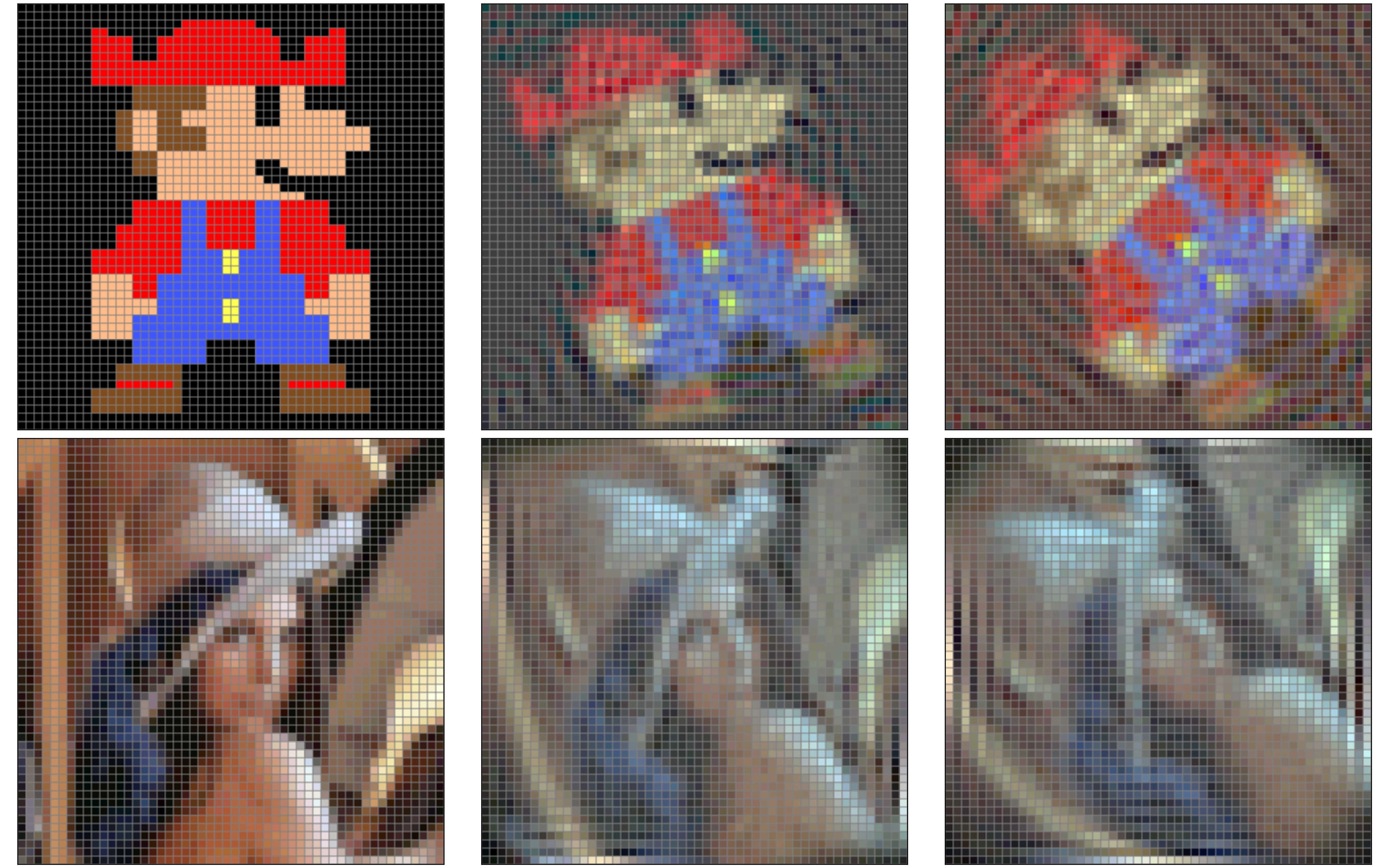
Figure 4: Left: Two RGB $52\times 52$ pixellated images (above a pseudo-Mario, below, the well-known Lena). Center and Right: Their unitary rotation by $\theta=\frac{1}{8}\pi$ and $\frac{1}{4}\pi$ with the normalization (29); the data image of the former can be further rotated by $\frac{1}{8}\pi$ to obtain the data-image of the latter, because the unitary transformations satisfy composition.

We should remark that the computation of all figure rotations in this report has been performed with an algorithm that enhances the speed of the previously used rotation algorithms [2, 5] that needs the computation of the special functions in the kernel (22). Previous reports of unitary transformations did not focus on the computational efficiency because one was more interested in the mathematical features of the transformations. Yet for example in [5] a grayscale rectangular image of $61\times 37=2257$ pixels was calculated in $\sim$78 hours, here each of the three layers of Fig. 4 has $52\times 52=2704$ pixels that were computed in $\sim$250 seconds, while the full RGB image took $\sim$12 minutes to complete. This improvement is due to two factors: first, the optimization of the routine to calculate the elements in (22) was done through a three-term recurrence relation (instead of library functions), and that a high-level scripting language such as Julia [20] was used, allowing the implementation of a syntactically natural transformation algorithm that simultaneously profits from the multi-threading in modern CPU’s. For more technical details, such as the binomial overflow as $N$ grows, the algorithm we used in all the previous figures is provided by an Open Source code shared on a public repository [8], to fulfill the principle of reproducibility for the results here presented.

4 Conclusions

We remarked above that the unitary rotation algorithm for pixellated images based on the finite oscillator model is unique, and can be inverted or concatenated. Yet we should underline that the unitary rotation algorithm requires that the value at every pixel in the rotated image depend on the values of all pixels of the input image. We are thus dealing with an $\mathcal{O}(N^{4})$ dependence in the number of operations needed to compute a rotation. The obvious advantage of information conservation comes thus at the price of a lengthier computation time. For commercial applications, where $N\approx 10^{3}$ is common, the more common image rotation algorithms based on interpolation in smaller regions of an image, have none of the former advantages, nor the last disadvantage.

The results presented for three basic colors of course also apply to any number of quantities that may be attached to the pixel values in pre-ordained ranges. The unitary rotations can also be made to act on the latter quantities covariantly, such as would be the case for a discrete and finite vector field, whose two components will rotate together with the data-image. Also, three- and higher-dimensional pixellated (‘voxellated’) images, subject to rotations [22] can be subject to considerations similar to those analyzed here.

Lastly, we should place the group of rotations of pixellated screens within the wider context of the finite oscillator model, which uses basically the rotation Lie subalgebra chain $\hbox{\sf so($3$)}\supset\hbox{\sf so($2$)}$ to provide the pixel coordinates and a phase space interpretation for the system, as opposed to their usual numbering through the $N$-point Fourier transform. In the latter, the position space forms a discrete torus whose two discrete $(x,y)$ coordinates curl into circles, but where rotations between them cannot be applied without breaking the torus. In the finite oscillator model, the manifold harboring the coordinates is a sphere, which can be freely rotated and also gyrated in phase space, among other linear canonical transformations.

References

- [1] N.M. Atakishiyev, L.E. Vicent and K.B. Wolf, Continuous vs. discrete fractional Fourier transforms, J. Comp. Appl. Math. 107, 73–95 (1999).
- [2] N.M. Atakishiyev, G.S. Pogosyan, L.E. Vicent, and K.B. Wolf, Finite two-dimensional oscillator II. The radial model, J. Phys. A 34, 9399–9415 (2001).
- [3] K.B. Wolf and L.E. Vicent, The Fourier U(2) group and separation of discrete variables, Sigma 7, 053, 18p. (2011).
- [4] N.M. Atakishiyev, G.S. Pogosyan, L.E. Vicent and K.B. Wolf, Finite two-dimensional oscillator. I: The Cartesian model, J. Phys. A 34, 9381–9398 (2001).
- [5] A.R. Urzúa and K.B. Wolf, Unitary rotation and gyration of pixellated images on rectangular screens, J. Opt. Soc. Am. A 33, 642–647 (2016).
- [6] N.M. Atakishiyev, G.S. Pogosyan, and K.B. Wolf, Finite models of the oscillator, Phys. Part. Nuclei 36, 521–555 (2005).
- [7] L.C. Biedenharn and J.D. Louck, Angular Momentum in Quantum Physics. Theory and Application. Encyclopedia of Mathematics and its Applications, Vol. 8 (Addison-Wesley Publ. Co., Reading, Mass.,1981).
- [8] A.R. Urzúa (2022), Polychromatic Unitary Rotations, version 0.1.0 [Computer software], in https://github.com/rurz/UnitRots.
- [9] K.B. Wolf, Integral Transforms in Science and Engineering (Plenum Press, New York, 1979).
- [10] C. van Trigt, Open problems in color constancy: discussion, J. Opt. Soc. Am. A 31, 338–347 (2014)
- [11] R.G. Kuehni, Color space and its divisions, Color Research & Application 26, 209–222 (2001).
- [12] I. Lissner and P. Urban, Toward a unified color space for perception-based image processing, IEEE Transactions on Image Processing 21, 1153–1168 (2012).
- [13] G. Wyszecki and W.S. Stiles, Color Science Vol. 8 (Wiley, New York, 1982).
- [14] S. Süsstrunk, R. Buckley, and S. Swen, Standard rgb color spaces, Color and Imaging Conference 1999, 127–134 (1999).
- [15] H-R. Kang,Color Technology for Electronic Imaging Devices, (SPIE Optical Engineering Press, Bellingham, Wash., 1997).
- [16] Z. Shen. Three-Color Tunable Organic Light-Emitting Devices, Science 276, 2009–2011 (1997).
- [17] R.W. Pridmore, Complementary colors: The structure of wavelength discrimination, uniform hue, spectral sensitivity, saturation, chromatic adaptation, and chromatic induction, Color Research & Application 34, 233–252 (2009).
- [18] R.W. Pridmore, Complementary colors: A literature review, Color Research & Application 46, 482–488 (2020).
- [19] A.R. Urzúa, “Rotaciones y giraciones en pantallas cartesianas rectangulares” (M.Sc. thesis, UNAM, 2016), https://repositorio.unam.mx/contenidos/95764.
- [20] J. Bezanson, A. Edelman, S. Karpinski, and V.B. Shah, Julia: A Fresh Approach to Numerical Computing. In: SIAM Review 59, 65–98 (2017). https://doi.org/10.1137/141000671.
- [21] H. Grassmann, Zur Theorie der Farbenmischung, Ann. Phys. Chem. 165, 69 (1853).
- [22] G. Krötzsch, K. Uriostegui and K.B. Wolf, Unitary rotations in two-, three-, and -dimensional Cartesian data arrays, J. Opt. Soc. Am. A 31, 1531–1535 (2014).