Split Electrons in Partition Density Functional Theory

Abstract

Partition Density Functional Theory (P-DFT) is a density embedding method that partitions a molecule into fragments by minimizing the sum of fragment energies subject to a local density constraint and a global electron-number constraint. To perform this minimization, we study a two-stage procedure in which the sum of fragment energies is lowered when electrons flow from fragments of lower electronegativity to fragments of higher electronegativity. The global minimum is reached when all electronegativities are equal. The non-integral fragment populations are dealt with in two different ways: (1) An ensemble approach (ENS) that involves averaging over calculations with different numbers of electrons (always integers); and (2) A simpler approach that involves fractionally occupying orbitals (FOO). We compare and contrast these two approaches and examine their performance in some of the simplest systems where one can transparently apply both, including simple models of heteronuclear diatomic molecules and actual diatomic molecules with 2 and 4 electrons. We find that, although both ENS and FOO methods lead to the same total energy and density, the ENS fragment densities are less distorted than those of FOO when compared to their isolated counterparts, and they tend to retain integer numbers of electrons. We establish the conditions under which the ENS populations can become fractional and observe that, even in those cases, the total charge transferred is always lower in ENS than in FOO. Similarly, the FOO fragment dipole moments provide an upper bound to the ENS dipoles. We explain why, and discuss implications.

I Introduction

Kohn-Sham Density Functional Theory (KS-DFT) Hohenberg and Kohn (1964); Kohn and Sham (1965); Parr and Weitao (1989), continues to be one of the most powerful and widely used methods to calculate the electronic properties of matter. Approximate exchange-correlation (XC) functionals used within KS-DFT suffer from various errors that limit its applicability Cohen, Mori-Sánchez, and Yang (2012). Among these errors, delocalization and static-correlation errors have been widely studied Cohen, Mori-Sánchez, and Yang (2008, 2012) but, in spite of several recent approaches to correct them Pederson, Ruzsinszky, and Perdew (2014); Kraisler and Kronik (2015); Nafziger and Wasserman (2015); Li et al. (2018); Perdew (2021); Kirkpatrick et al. (2021), there is still no general, robust method that works reliably in practice.

When dissociating a molecule into its constituent atoms, most approximate XC functionals will minimize the energy by placing fractional numbers of electrons on the separated atoms. The differences between these fractional numbers and the correct integers, referred to here as the “fractional-charge error" (FCE), are sometimes taken as a measure of the delocalization error (DE) Mori-Sánchez, Cohen, and Yang (2008). But the DE, whose origin is the incorrect delocalization of electron densities, is not only present at dissociation. It is also present at any set of internuclear separations, for which the concept of ‘atomic electron number’ is no longer valid (i.e. there is no unique way to assign electrons to any particular nucleus in the molecule). Although the FCE is only well defined at dissociation, one can show (see for example Figure 2) that the error in the energy associated to the FCE settles in long before reaching dissociation when the ‘atoms’ are still at interacting distances and their electronic densities cannot be understood separately. Theories that provide a definite prescription for calculating fragment populations at finite internuclear separations are thus useful in this context Cohen and Wasserman (2006); Tang, Nafziger, and Wasserman (2012); Fabiano, Laricchia, and Sala (2014); Schulz and Jacob (2019).

Partition-DFT (P-DFT) Cohen and Wasserman (2007); Elliott et al. (2010); Nafziger and Wasserman (2014) is a formally exact density embedding method that leads to such a definite prescription, and can thus be used to link the DE and the FCE at any set of internuclear separations. There are two sensible ways for treating fractional electron numbers in P-DFTNafziger, Jiang, and Wasserman (2017); Jiang, Nafziger, and Wasserman (2018): (1) An ensemble approach (ENS) that involves averaging over calculations with different numbers of electrons (always integers); and (2) A simpler approach that involves fractionally occupying KS orbitals (FOO). In this work, we compare and contrast these two approaches and examine their performance in some of the simplest systems where one can transparently apply both.

All of the P-DFT calculations of fractional charges done to date Cohen et al. (2009); Elliott et al. (2009); Tang, Nafziger, and Wasserman (2012); Oueis and Wasserman (2018); Nafziger and Wasserman (2014); Nafziger, Jiang, and Wasserman (2017) have been carried out on model systems of non-interacting Cohen et al. (2009); Elliott et al. (2009); Tang, Nafziger, and Wasserman (2012) or one-dimensional interacting Oueis and Wasserman (2018) electrons. Whenever 3D P-DFT calculations have involved fractional charges, the molecules studied have been centro-symmetric (homonuclear diatomics), not involving ground-state charge transfer between the constituent atoms Nafziger and Wasserman (2014); Nafziger, Jiang, and Wasserman (2017). We present here the first calculations on 3D heteronuclear diatomic molecules and ions. Our goal is to examine how the two methods for splitting electrons between fragments (ENS and FOO) differ in practice. In Sec.II, we review the theory highlighting the role of electronegativity equalization and show how this important condition plays differently in FOO and ENS. In Sec.III we present P-DFT calculations on 3D heteronuclear diatomic molecules with 1, 2, and 4 electrons, and show that, even though both ENS and FOO methods lead to the same total molecular densities, they lead to different descriptions of the charge transferred between fragments.

II Partition-DFT and two alternative methods for determining fractional electron numbers

To highlight the role of fractional populations in P-DFT, we begin with a description of P-DFT in which the $\{N_{\alpha}\}$ ($\alpha$ is used to label fragments) are presumed fixed and known in advance. We will then describe how to optimize the set $\{N_{\alpha}\}$, but - as a first step - we consider these numbers as given, for example, by a calculation of formal charges from any of the many methods available for that purpose Mulliken (1955); Hirshfeld (1977); Reed, Weinstock, and Weinhold (1985); Bader (1990); Rousseau, Peeters, and Van Alsenoy (2001).

For a system of $N_{M}$ electrons subject to an external potential $v\left(\mathbf{r}\right)$ (due to all the nuclei), this potential can be divided as

$$v\left(\mathbf{r}\right)=\underset{\alpha=1}{\overset{N_{f}}{\sum}}v_{\alpha}\left(\mathbf{r}\right),$$ (1)

where $v_{\alpha}\left(\mathbf{r}\right)$ is the external potential of the $\alpha^{\rm th}$ fragment and $N_{f}$ is the number of fragments. The task of P-DFT is to minimize the sum of fragment energies

$$E_{f}\left[\left\{n_{\alpha}\right\}\right]\equiv\underset{\alpha=1}{\overset{N_{f}}{\sum}}E_{\alpha}\left[n_{\alpha}\right]$$ (2)

subject to the set of constraints specified below (Eqs.(3-4)). In Eq.(2), $E_{\alpha}\left[n_{\alpha}\right]$ and $n_{\alpha}\left(\mathbf{r}\right)$ are the ground-state energy and density of the $\alpha^{\rm th}$ fragment. Given a set $\{N_{\alpha}\}$ satisfying $\underset{\alpha=1}{\overset{N_{f}}{\sum}}N_{\alpha}=N_{M}$, where the total number of electrons $N_{M}$ is an integer, the total ground-state density $n_{M}\left(\mathbf{r}\right)$ is optimally partitioned when $E_{f}$ is minimized with respect to variations of the $\left\{n_{\alpha}\right\}$ subject to the $N_{f}+1$ independent constraints:

$$n_{M}\left(\mathbf{r}\right)=\underset{\alpha=1}{\overset{N_{f}}{\sum}}n_{\alpha}\left(\mathbf{r}\right),$$ (3)

$$N_{\alpha}=\intop n_{\alpha}\left(\mathbf{r}\right)d\mathbf{r},\;\forall\alpha\in\left\{1,\cdots,N_{f}\right\}.$$ (4)

Because the $N_{\alpha}$ can be non-integer, $E_{\alpha}\left[n_{\alpha}\right]$ needs to be defined for non-integer electron numbers. Two alternative methods for accomplishing this are described in Sections II-A and II-B. In either case, the constrained search for an optimum $\{n_{\alpha}\}$ for fixed $\{N_{\alpha}\}$ can be formally converted into the unconstrained minimization of a grand-potential $G\left[\left\{n_{\alpha}\right\},v_{p}\left(\mathbf{r}\right),\left\{\chi_{\alpha}\right\}\right]$, where the partition potential $v_{p}(\mathbf{r})$ and fragment electronegativities $\left\{\chi_{\alpha}\right\}$ are the Lagrange multipliers associated to constraints (3) and (4), respectively:

$$G \left[\left\{n_{\alpha}\right\},v_{p}\left(\mathbf{r}\right),\left\{\chi_{\alpha}\right\}\right]=E_{f}\left[\left\{n_{\alpha}\right\}\right]+\int v_{p}\left(\mathbf{r}\right)\times$$ (5)

$$\left(\underset{\alpha}{\sum}n_{\alpha}\left(\mathbf{r}\right)-n_{M}\left(\mathbf{r}\right)\right)d\mathbf{r}+\underset{\alpha}{\sum}\chi_{\alpha}\left(\int n_{\alpha}\left(\mathbf{r}\right)d\mathbf{r}-N_{\alpha}\right).$$

The Euler-Lagrange equation for the $\alpha^{\rm th}$ fragment can be obtained by minimizing $G\left[\left\{n_{\alpha}\right\},v_{p}\left(\mathbf{r}\right),\left\{\chi_{\alpha}\right\}\right]$ with respect to the corresponding fragment density $n_{\alpha}\left(\mathbf{r}\right)$, i.e., $\frac{\delta G}{\delta n_{\alpha}\left(\mathbf{r}\right)}=0$, yielding

$$\chi_{\alpha}=-\left(\frac{\delta E_{\alpha}\left[n_{\alpha}\right]}{\delta n_{\alpha}\left(\mathbf{r}\right)}+v_{p}\left(\mathbf{r}\right)\right),$$ (6)

where $\frac{\delta E_{\alpha}\left[n_{\alpha}\right]}{\delta n_{\alpha}\left(\mathbf{r}\right)}$ needs to be well defined for non-integer electron numbers (see Secs.II-A and II-B).

The $v_{p}\left(\mathbf{r}\right)$ for fixed $\{N_{\alpha}\}$ is unique Cohen and Wasserman (2006, 2007); Huang, Pavone, and Carter (2011), but $E_{f}$ can generally be lowered further by transferring a fraction of an electron from a fragment of lower electronegativity to one of higher electronegativity. The global minimum of $E_{f}$ is then found when all fragment electronegativities are equal Cohen and Wasserman (2006, 2007), i.e. $\chi_{\alpha}=\chi^{*},\forall\alpha$, where $\chi^{*}$ is a common optimal electronegativity. Then the constraints (4) unify into:

$$N_{M}=\underset{\alpha=1}{\overset{N_{f}}{\sum}}\intop n_{\alpha}\left(\mathbf{r}\right)d^{3}\mathbf{r},$$ (7)

and the grand potential $G\left[\left\{n_{\alpha}\right\},v_{p}\left(\mathbf{r}\right),\left\{\chi_{\alpha}\right\}\right]$ becomes

$$G \left[\left\{n_{\alpha}\right\},v_{p}\left(\mathbf{r}\right),\chi^{*}\right]=E_{f}\left[\left\{n_{\alpha}\right\}\right]+\int v_{p}\left(\mathbf{r}\right)\times$$ (8)

$$\left(\underset{\alpha}{\sum}n_{\alpha}\left(\mathbf{r}\right)-n_{M}\left(\mathbf{r}\right)\right)d^{3}\mathbf{r}+\chi^{*}\left(\underset{\alpha}{\sum}\int n_{\alpha}\left(\mathbf{r}\right)d^{3}\mathbf{r}-N_{M}\right)$$

with $\chi^{*}=-\left(\frac{\delta E_{f}\left[\left\{n_{\alpha}\right\}\right]}{\delta n_{M}\left(\mathbf{r}\right)}+v_{p}\left(\mathbf{r}\right)\right)$.

Thus, by varying the $\left\{N_{\alpha}\right\}$, we can determine the optimal fragment electron populations for which all fragment electronegativities are equal and the grand-potential is minimized to:

$$E_{f}^{*}=\underset{\left\{\chi_{\alpha}\right\}}{\min}\underset{\left\{n_{\alpha}\right\}}{\min}G\left[\left\{n_{\alpha}\right\},v_{p}\left(\mathbf{r}\right),\left\{\chi_{\alpha}\right\}\right]$$ (9)

A general, simple algorithm for Eq.(9) can be formulated: Start with a guess for $\left\{N_{\alpha}\right\}$ and do self-consistent calculations to obtain all fragment electronegativities $\left\{\chi_{\alpha}\right\}$. Then update the $\left\{N_{\alpha}\right\}$ by using $N_{\alpha}^{\left(k+1\right)}=N_{\alpha}^{\left(k\right)}+\Gamma\left(\chi_{\alpha}^{\left(k\right)}-\bar{\chi}^{\left(k\right)}\right)$ Elliott et al. (2010), where $\Gamma$ is an appropriate positive constant and $\bar{\chi}^{(k)}$ is the average of all fragment electronegativities for the $k^{\rm th}$ iteration. The process is iterated until $\chi_{\alpha}^{\left(k\right)}-\bar{\chi}^{\left(k\right)}$ falls below an acceptable threshold. The resulting $\{N_{\alpha}\}$ will be referred to as optimal and be denoted as $\{N_{\alpha}^{*}\}$ from now on. We now turn our attention to two alternative methods for treating non-integer electron numbers.

II.1 Fractional Orbital populations (FOO)

The density of the $\alpha^{\rm th}$ fragment can be constructed as

$$n_{\alpha}^{\rm FOO}\left(\mathbf{r}\right)=\underset{i}{\sum}f_{\alpha,i}\left|\phi_{\alpha,i}\left(\mathbf{r}\right)\right|^{2},$$ (10)

where $\underset{i}{\sum}f_{\alpha,i}=N_{\alpha}$, and $f_{\alpha,i}$ is the occupation number for $\phi_{\alpha,i}\left(\mathbf{r}\right)$ (the $i^{\rm th}$ KS orbital of the $\alpha^{\rm th}$ fragment). Since we only consider the ground state, $f_{\alpha,i}=1$ for all occupied orbitals except for the highest occupied molecular orbital (HOMO), in which case $0<f_{\alpha}^{\rm HOMO}\leq 1$. The non-interacting kinetic energy is calculated by Janak (1978)

$$T_{s}^{\mathrm{FOO}}\left[n_{\alpha}\right]=-\frac{1}{2}\underset{i}{\sum}f_{\alpha,i}\int\phi_{\alpha,i}^{*}\left(\mathbf{r}\right)\nabla^{2}\phi_{\alpha,i}\left(\mathbf{r}\right)d\mathbf{r}.$$ (11)

The energy of the $\alpha^{\rm th}$ fragment $E_{\alpha}\left[n_{\alpha}\right]$ is then defined in the same way as in KS-DFT (we drop the “FOO" superscript from the densities for notational simplicity),

$$E_{\alpha}\left[n_{\alpha}\right]=T_{s}^{\mathrm{FOO}}\left[n_{\alpha}\right]+E_{\mathrm{HXC}}\left[n_{\alpha}\right]+\int v_{\alpha}\left(\mathbf{r}\right)n_{\alpha}\left(\mathbf{r}\right)d\mathbf{r},$$ (12)

where $E_{\mathrm{H}}\left[n_{\alpha}\right]$ and $E_{\mathrm{XC}}\left[n_{\alpha}\right]$ are the Hartree and exchange-correlation energies of the $\alpha^{\rm th}$ fragment. Then the Euler-Lagrange equation (6) becomes

$$\chi_{\alpha}^{\rm FOO}=-\left(\frac{T_{s}^{\mathrm{FOO}}\left[n_{\alpha}\right]}{\delta n_{\alpha}\left(\mathbf{r}\right)}+v_{\mathrm{HXC}}\left[n_{\alpha}\right]\left(\mathbf{r}\right)+v_{\alpha}\left(\mathbf{r}\right)+v_{p}\left(\mathbf{r}\right)\right).$$ (13)

In the same way as in KS-DFT Parr and Weitao (1989), one can derive the KS equations for the $\alpha^{\rm th}$ fragment:

$$\left\{-\frac{1}{2}\nabla^{2}+v_{\alpha}^{\mathrm{eff}}\left[n_{\alpha}\right]\left(\mathbf{r}\right)+v_{p}\left(\mathbf{r}\right)\right\}\phi_{\alpha,i}\left(\mathbf{r}\right)=\epsilon_{\alpha,i}\phi_{\alpha,i}\left(\mathbf{r}\right),$$ (14)

where the fragment effective potential is

$$v_{\alpha}^{\mathrm{eff}}\left[n_{\alpha}\right]\left(\mathbf{r}\right)=v_{\alpha}\left(\mathbf{r}\right)+v_{\mathrm{HXC}}\left[n_{\alpha}\right]\left(\mathbf{r}\right).$$ (15)

The fragment KS equations for the $\alpha^{\rm th}$ fragment can be regarded as those for $N_{\alpha}$ electrons subject to the external potential $v_{\alpha}\left(\mathbf{r}\right)+v_{p}\left(\mathbf{r}\right)$. Therefore, we define the total energy for the $\alpha^{\rm th}$ fragment as

$$\widetilde{E}_{\alpha}\left[n_{\alpha}\right]\equiv E_{\alpha}\left[n_{\alpha}\right]+\int v_{p}\left(\mathbf{r}\right)n_{\alpha}\left(\mathbf{r}\right)d\mathbf{r}.$$ (16)

Considering that $N_{\alpha}$ is continuous and the energy is differentiable, we use the definition of electronegativity given by Iczkowski and Margrave Iczkowski and Margrave (1961), i.e., $\chi_{\alpha}=-\frac{\partial\widetilde{E}_{\alpha}}{\partial N_{\alpha}}$. It is straightforward to prove that the energy functional $\widetilde{E}_{\alpha}\left[n_{\alpha}\right]$ is differentiable Englisch and Englisch (1984a, b) and $\chi_{\alpha}^{\rm FOO}=-\frac{\delta\widetilde{E}_{\alpha}\left[n_{\alpha}\right]}{\delta n_{\alpha}\left(\mathbf{r}\right)}=-\frac{\partial\widetilde{E}_{\alpha}}{\partial N_{\alpha}}$ Parr and Weitao (1989); Ripka, Blaizot, and Ripka (1986). Furthermore, according to Janak’s theorem Janak (1978), we know that $\frac{\partial\widetilde{E}_{\alpha}}{\partial N_{\alpha}}=\epsilon_{\alpha}^{\mathrm{HOMO}}$. Thus, we obtain $\chi_{\alpha}^{\rm FOO}=-\epsilon_{\alpha}^{\mathrm{HOMO}}$.

II.2 Ensembles (ENS)

Alternatively, when $N_{\alpha}$ lies between the integers $p_{\alpha}$ ($=\left\lfloor N_{\alpha}\right\rfloor$) and $p_{\alpha+1}$, we can write the $\alpha$-density as:

$$n_{\alpha}^{\rm ENS}\left(\mathbf{r}\right)=\left(1-\omega_{\alpha}\right)n_{p_{\alpha}}\left(\mathbf{r}\right)+\omega_{\alpha}n_{p_{\alpha}+1}\left(\mathbf{r}\right),$$ (17)

emulating known results for the exact extension of DFT to non-integer electron numbers Perdew et al. (1982) (true for the exact XC-functional). A related approach Kraisler and Kronik (2015) has been shown to be useful in eliminating the asymptotic fractional dissociation problem of the Local Density Approximation (LDA). In Eq.(17), the two ensemble component densities $n_{p_{\alpha}}\left(\mathbf{r}\right)$ and $n_{p_{\alpha+1}}\left(\mathbf{r}\right)$ integrate to $p_{\alpha}$ and $p_{\alpha+1}$ electrons, respectively, and $0<\omega_{\alpha}<1$ so that $N_{\alpha}=p_{\alpha}+\omega_{\alpha}$.

The corresponding fragment energy is

$$E_{\alpha}\left[n_{\alpha}\right]=\left(1-\omega_{\alpha}\right)E_{\alpha}\left[n_{p_{\alpha}}\right]+\omega_{\alpha}E_{\alpha}\left[n_{p_{\alpha}+1}\right],$$ (18)

where $E_{\alpha}\left[n_{p_{\alpha}}\right]$ and $E_{\alpha}\left[n_{p_{\alpha}+1}\right]$ are the ground-state energies for $p_{\alpha}$ and $p_{\alpha}+1$ electrons subject to an external potential $v_{\alpha}\left(\mathbf{r}\right)+v_{p}\left(\mathbf{r}\right)$.

Since the allowed density variations must now keep $p_{\alpha}$ electrons in $n_{p_{\alpha}}(\mathbf{r})$ and $p_{\alpha+1}$ electrons in $n_{p_{\alpha+1}}(\mathbf{r})$, the constraints (4) turn into $2N_{f}$ independent constraints, and the Lagrange multipliers $\{\chi_{\alpha}\}$ can be replaced by a pair-set of multipliers $\{\lambda_{p_{\alpha}},\lambda_{p_{\alpha}+1}\}$. The grand-potential in Eq.(5), now $G^{\mathrm{ENS}}\left[\left\{n_{\alpha}\right\},v_{p}\left(\mathbf{r}\right),\left\{\lambda_{p_{\alpha}},\lambda_{p_{\alpha}+1}\right\}\right]$, is minimized with respect to variations of the $n_{p_{\alpha}}(\mathbf{r})$ and $n_{p_{\alpha+1}}(\mathbf{r})$, yielding

$$\lambda_{p_{\alpha}}=-\left(\frac{\delta E_{\alpha}\left[n_{p_{\alpha}}\right]}{\delta n_{p_{\alpha}}\left(\mathbf{r}\right)}+v_{p}\left(\mathbf{r}\right)\right),$$ (19)

and a companion equation for $\lambda_{p_{\alpha}+1}$. Expressing $E_{\alpha}\left[n_{p_{\alpha}}\right]$ in terms of KS quantities, Eq.(14) is now replaed by a pair of analogous KS equations in which all of the $\alpha$-subindices in Eq.(14) are replaced by either $p_{\alpha}$ or $p_{\alpha}+1$. The fragment effective potential $v_{p_{\alpha}}^{\mathrm{eff}}\left[n_{p_{\alpha}}\right]\left(\mathbf{r}\right)$ has the same decomposition as in Eq.(15), but the Hartree and XC-potentials are now evaluated at the appropriate integer-number densities. These in turn are constructed simply by summing over the $p_{\alpha}$ (or $p_{\alpha+1}$) occupied KS orbitals.

For atoms and molecules, $\epsilon_{p_{\alpha}}^{\mathrm{HOMO}}<\epsilon_{p_{\alpha}+1}^{\mathrm{HOMO}}$ and $\lambda_{p_{\alpha}}>\lambda_{p_{\alpha}+1}$, since $p_{\alpha}$ and $p_{\alpha}+1$ electrons are subjected to the same external potential $v_{\alpha}\left(\mathbf{r}\right)+v_{p}\left(\mathbf{r}\right)$. Defining the total energy for the $\alpha^{\rm th}$ fragment in the same way as Eq. (16), we now find for the electronegativity Perdew et al. (1982):

$$\chi_{\alpha}^{\rm ENS}=\widetilde{E}_{\alpha}\left[n_{p_{\alpha}}\right]-\widetilde{E}_{\alpha}\left[n_{p_{\alpha}+1}\right]~{}~{}~{}~{}~{}~{}(0<\omega_{\alpha}<1).$$ (20)

If $N_{\alpha}$ is an integer, $\chi_{\alpha}^{\rm ENS}$ is strictly undefined (but one can consider right- and left- limits for it, as will be discussed in Sec.III-B).

II.3 HOMO Energy and Electronegativity: FOO vs. ENS

The one-electron nature of the KS equations leads to densities for finite systems that decay asymptotically as Levy, Perdew, and Sahni (1984); Parr and Weitao (1989)

$$n\left(\mathbf{r}\right)\underset{r\rightarrow\infty}{\longrightarrow}e^{-2\kappa r},$$ (21)

where $\kappa=\sqrt{-2\left(\epsilon^{\mathrm{HOMO}}-v_{\mathrm{XC}}\left(\infty\right)\right)}$. If $v_{\mathrm{XC}}\left(\mathbf{r}\right)\underset{r\rightarrow\infty}{\longrightarrow}0$, then $\kappa=\sqrt{-2\epsilon^{\mathrm{HOMO}}}$. LDA and GGA densities satisfy this condition.

Due to the density constraint of Eq.(3), we see that if the fragment densities have different exponential decay rates, at least one of them (fragment $\alpha^{*}$) must match the decay of the total density in the asymptotic region. Using FOO, this implies $\epsilon_{\alpha^{*}}^{\mathrm{HOMO}}=\epsilon_{M}^{\mathrm{HOMO}}=const$. By using $\chi_{\alpha}^{\rm FOO}=-\epsilon_{\alpha}^{\mathrm{HOMO}}$ (see last line of Sec.II-A), we find that $\chi_{\alpha^{*}}^{\rm FOO}=-\epsilon_{M}^{\mathrm{HOMO}}$. When $E_{f}$ reaches its global minimum, all fragment electronegativities are equal, so $\chi_{\alpha}=-\epsilon_{M}^{\mathrm{HOMO}}$ for all $\alpha$. Therefore, the best way to approach the global minimum of $E_{f}$ is to always assign less electrons to fragments whose electronegativities are $\chi_{M}$ and more electrons to fragments whose electronegativities are larger than $\chi_{M}$. In this way, the iteration formula in the algorithm for Eq. (9) can be modified for the $(k+1)^{\rm th}$ iteration as follows: For fragments whose $\chi_{\alpha}^{\left(k\right)}>\chi_{M}$, set $N_{\alpha}^{\left(k+1\right)}=N_{\alpha}^{\left(k\right)}+\Gamma\left(\chi_{\alpha}^{\left(k\right)}-\chi_{M}\right)$; for fragments whose $\chi_{\alpha}^{\left(k\right)}=\chi_{M}$, set $N_{\alpha}^{\left(k+1\right)}=N_{\alpha}^{\left(k\right)}$ or $N_{\alpha}^{\left(k+1\right)}=N_{M}-\underset{\beta\neq\alpha}{\sum}N_{\beta}^{\left(k\right)}$.

In contrast, when using the ENS method of Sec.II-B, we find $\epsilon_{p_{\alpha^{*}+1}}^{\mathrm{HOMO}}=\epsilon_{M}^{\mathrm{HOMO}}=const$, and there is no direct relation between the fragment electronegativity $\chi_{\alpha}^{\rm ENS}$ of Eq.(20) and the molecular HOMO energy.

Finally, we note a key difference between the partition potentials of ENS and FOO: Assume the population of the $\alpha^{\rm th}$ fragment is non-integral and $\epsilon_{\alpha,\mathrm{FOO}}^{\mathrm{HOMO}}=\epsilon_{M}^{\mathrm{HOMO}}$, then we know $\varepsilon_{\alpha,\mathrm{ENS}}^{\mathrm{HOMO}}\leq\varepsilon_{M}^{\mathrm{HOMO}}$. Since there are $N_{\alpha}$ electrons subject to $v_{\alpha}\left(\mathbf{r}\right)+v_{p}^{\mathrm{FOO}}\left(\mathbf{r}\right)$ in FOO while there are $\left\lfloor N_{\alpha}\right\rfloor+1$ electrons subject to $v_{\alpha}\left(\mathbf{r}\right)+v_{p}^{\mathrm{ENS}}\left(\mathbf{r}\right)$ in ENS, $v_{p}^{\mathrm{ENS}}\left(\mathbf{r}\right)$ needs to be deeper than $v_{p}^{\mathrm{FOO}}\left(\mathbf{r}\right)$ to account for the fact that $\left\lfloor N_{\alpha}\right\rfloor+1>N_{\alpha}$, and thus $\int v_{p}^{\mathrm{ENS}}\left(\mathbf{r}\right)n_{M}\left(\mathbf{r}\right)d\mathbf{r}<\int v_{p}^{\mathrm{FOO}}\left(\mathbf{r}\right)n_{M}\left(\mathbf{r}\right)d\mathbf{r}$. As a consequence, $E_{p}^{\mathrm{ENS}}$ is more negative than $E_{p}^{\mathrm{FOO}}$ and, since FOO and ENS must yield the same total energy, $E_{f}^{\mathrm{ENS}}$ will be less negative than $E_{f}^{\mathrm{FOO}}$. All of these findings are illustrated below.

III Examples and Discussion

We now illustrate the preceding discussions on a few model systems of diatomic molecules and on actual diatomic molecules. In all cases, the nuclei are separated a distance $R$ and located at $-(R/2)\hat{z}$ and $+(R/2)\hat{z}$ along the $z$-axis. All calculations are performed on a prolate-spheroidal real-space grid Becke (1982); Nafziger and Wasserman (2014). Considering the azimuthal symmetry of diatomic molecules, we only need to solve the Kohn-Sham equations on a two-dimensional mesh. Libxc library Marques, Oliveira, and Burnus (2012) is used to evaluate approximate exchange correlation functionals.

We partition the molecules into two fragments, labeled $A$ and $B$, and denote the optimal electron populations by $N_{A}^{*}$ and $N_{B}^{*}$. When isolated ($R\to\infty$), the correct populations are denoted by $N_{A}^{0}$ and $N_{B}^{0}$, so we can define the number of electrons transferred from $A$ to $B$ as $\Delta N=N_{A}^{0}-N_{A}^{*}=N_{B}^{*}-N_{B}^{0}$. When no superscript is used for $N_{A}$ and $N_{B}$, it should be understood that the numbers have been fixed, but not optimized (i.e. they do not minimize $E_{f}$).

III.1 One electron: Model of a one-electron molecule $\mathbf{AB^{+Z_{B}}}$

We first consider a one-electron diatomic molecular ion $\mathrm{AB^{+Z_{B}}}$ with nuclear charges $Z_{A}=1$ and variable $Z_{B}<1$, so that the dissociated molecule consists of a hydrogen atom and a “proton" of charge $+Z_{B}$. (In the discussion below, we sometimes refer to $\Delta Z\equiv 1-Z_{B}$). A similar model but in 1D and with delta-function potentials was studied in ref.Cohen et al. (2009). The exact P-DFT solution reported here for Coulomb potentials in 3D leads to well-localized fragment densities for all $R$ (see Figure 1), just like in the 1D model of ref.Cohen et al. (2009). As the molecule is stretched, an electron is smoothly transferred from $B$ to $A$. (What we mean by “smoothly" will be clarified below, see the right panel of Fig.2).

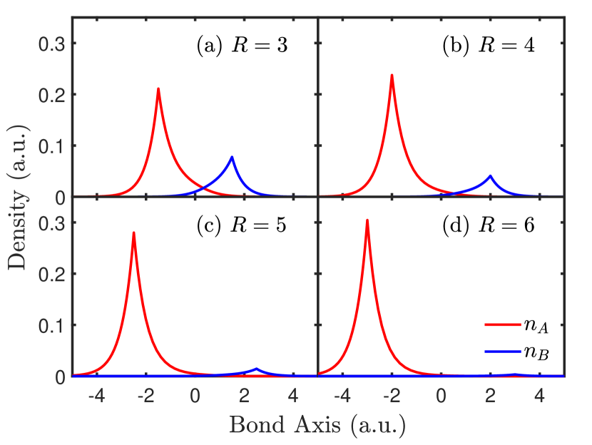
Figure 1: The optimal electron densities of fragments along the bond axis for model molecule $\mathrm{AB}^{+0.9}$ ($Z_{A}=1$ and $Z_{B}=0.90$) with the exact functional when the internuclear distance is $R=$ (a) 3.0, (b) 4.0, (c) 5.0, and (d) 6.0 a.u..

The left panel of Fig.2 compares the exact and LDA dissociation curves of $\mathrm{AB^{+Z_{B}}}$, showing a vivid example of LDA fractional-charge and delocalization errors. The equilibrium distance $R_{\rm eq}$ is about 2 a.u. for the exact solution and about 2.3 a.u. for the LDA ($R_{\rm eq}$ is approximately constant in the range $0.9<Z_{B}<1$). Two lessons can be drawn from the left panel of Fig. 2:

(1) The bond is stronger for the homonuclear case than it is for the heteronuclear case. The larger the value of $\Delta Z$, the weaker the binding, as explained beautifully in Chapter 10 of ref.Feynman, Sands, and Leighton (2011).

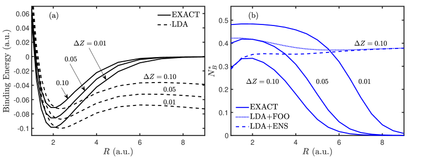
Figure 2: Binding energies (left) and optimal population of fragment B (right) for the model of a one-electron heteronuclear diatomic molecule $\mathrm{AB^{+Z_{B}}}$ (Sec.III-A) with the exact functional (solution) and LDA for $Z_{A}=1$, and $Z_{B}=0.90,0.95,0.99$. FOO and ENS results lead to identical binding energies, but $N_{B}^{*}$ differs when using the LDA as indicated in the right panel

.

(2) The LDA error manifests most clearly at the dissociation limit as the binding energy $E_{b}$ goes incorrectly to a negative value ($E_{b}$ is defined as the difference between the ground-state energy of the molecule and the sum of the ground-state energies of the isolated atoms, in this case just a hydrogen atom, so should be zero at dissociation). Furthermore, Figure 2 shows that this error increases as $\Delta Z\to 0$. In the limiting case of $\Delta Z=0$ (i.e. H${}_{2}^{+}$), the error has been well studied Perdew and Zunger (1981); Cohen, Mori-Sánchez, and Yang (2008) and understood as due to the incorrect treatment of fractional charges by the LDA. A hallmark of the delocalization error (DE) for a heteronuclear diatomic molecule is that the approximate functional incorrectly minimizes the total energy by placing fractional charges on the separated atoms. These incorrect fractional charges are well defined at dissociation. An interesting question arises here: The (incorrect) fractional charges that determine the DE are strictly only well defined at dissociation, as mentioned in the Introduction, but the left panel of Figure 2 shows that the DE settles in slowly as $R\gtrsim 4$. How do the fractional charges at finite $R$ evolve into those at dissociation as $R\to\infty$?

The right panel of Fig.2 provides the answer given by Partition-DFT through both ENS and FOO methods described in Sec.II, using both the exact functional ($E_{\mathrm{XC}}^{\mathrm{EXACT}}[n]=-E_{\mathrm{H}}[n]$ for one electron) and the LDA. For the exact case, ENS and FOO fragments are identical. The number of electrons in the $B$-fragment ($N_{B}$) reaches a maximum value for small $R$ and decreases monotonically down to zero at dissociation in the same way as was observed for the 1D model system of ref.Cohen et al. (2009). However, in the case of an approximate functional like the LDA, though FOO and ENS yield the same total molecular density and energy, they yield different fragment energies and densities. The ENS-LDA $N_{B}$ values are close to the exact ones for very small internuclear separations and around the maximum of $N_{B}$, but they do not decrease as $R$ grows and stay approximately constant for $R\gtrsim 4$, suggesting that the error in $N_{B}$ encodes the error in $E_{b}$. The FOO-LDA $N_{B}$ values converge to those of ENS-LDA as $R$ grows, but differ significantly for small $R$.

To discuss the origin of these differences, we take the case of $Z_{B}=0.9$ as an example, and fix $R=2.0$ a.u. (close to equilibrium).

FOO: The LDA electronegativities $\chi_{A}$ and $\chi_{B}$, as defined below Eq.(16), become equal when $N_{A}^{*}=0.5830$ (for the exact case, they equalize at $N_{A}^{*}=0.6654$, so the LDA error for the optimum occupation is -12%). This number is also the minimizer of $E_{f}$ (see bottom panels of Fig.3). When $N_{A}<N_{A}^{*}$, the electronegativity of $B$ equals $-\epsilon_{M}^{\mathrm{HOMO}}$, a constant value. In this range, $\chi_{A}>\chi_{B}$, so fragment $A$ has a higher tendency than $B$ to attract electrons: $B$ is the donor (“base") and $A$ is the acceptor (“acid"). As electrons are transferred from $B$ to $A$, both the electronegativity difference $\chi_{A}-\chi_{B}$ and $E_{f}$ decrease. On the other hand, when $N_{A}>N_{A}^{*}$, fragment $A$ and $B$ swap their donor/acceptor roles.

ENS: The LDA electronegativities now cross at $N_{A}^{*}=0.6485$. By switching from FOO to ENS, the magnitude of the error in $N_{A}^{*}$ has thus been reduced from 12% to 2%. The HOMO energy of the molecule equals the HOMO energy of one of the two fragments. That fragment is $A$ when $N_{A}>N_{A}^{**}$ and $B$ when $N_{A}<N_{A}^{**}$, where $N_{A}^{**}$ is the crossing point of the fragment HOMO energies, which differs slightly from $N_{A}^{*}$ (the crossing point for the electronegativities). In the case of Fig.3 (see inset in top right panel), $N_{A}^{**}=0.6630$.

This example indicates that the FOO method leads to a larger estimate than ENS for the charge transferred. In the case of Fig.(3), $\Delta N^{\mathrm{FOO}}=0.4170$ and $\Delta N^{\mathrm{ENS}}=0.3515$.

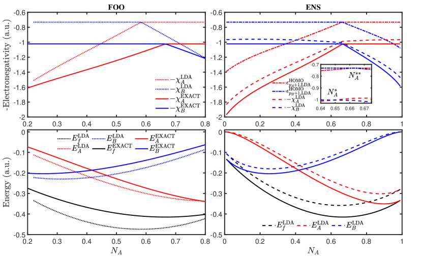
Figure 3: Negative electronegativities of fragments (top panels) and fragment energies and their sum (bottom panels) as a function of $N_{A}$ for the one-electron model molecule $\mathrm{AB^{+0.9}}$ of Sec.III-A ($Z_{A}=1$ and $Z_{B}=0.9$; at internuclear distance $R=2.0$ a.u.. $\epsilon^{\mathrm{HOMO}}_{M,\mathrm{LDA}}=-0.7311$ a.u. and $\epsilon^{\mathrm{HOMO}}_{M,\mathrm{EXACT}}=-1.0216$ a.u.) with LDA and exact functionals. Left panels: FOO. Right panels: ENS.

Now we note another qualitative difference between the two methods for calculating fractional populations: The ENS-LDA values of $E_{f}$ are above the exact ones, but the FOO-LDA values are below. This behavior can be traced back to an increased delocalization of the LDA-FOO densities when compared to ENS (see Figure 4), which in turn leads to an increased magnitude for the (negative) electron-nuclear interaction energy in FOO. This observation agrees with our analysis in Sec.II-C.

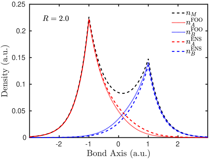
Figure 4: Fragment densities of the one-electron model molecule $\mathrm{AB^{+0.9}}$ ($Z_{A}=1$ and $Z_{B}=0.9$) along the bond axis at optimal electron populations with FOO+LDA and ENS+LDA when the internuclear distance is $R=2.0$ a.u..

Setting the bond mid-point as the origin, we define fragment electronic dipole moments as $\mathbf{p}_{\alpha}=\int\mathbf{r}n_{\alpha}\left(\mathbf{r}\right)d\mathbf{r}$. Then, $\mathbf{p}_{A}^{\mathrm{FOO}}=0.4219>0.3962=\mathbf{p}_{A}^{\mathrm{ENS}}$ and $\left|\mathbf{p}_{B}^{\mathrm{FOO}}\right|=\left|-0.2942\right|>\left|-0.2685\right|=\left|\mathbf{p}_{B}^{\mathrm{ENS}}\right|$. Clearly, the FOO fragments are more polarized than the ENS fragments.

III.2 Two electrons: Model of a two-electron molecule $\mathbf{AB^{+\delta}}$

We now add one more electron and allow both electrons to fully interact with each other and with the two nuclei. To keep the system bound in the LDA, this time we fix $Z_{B}=1$ and let $Z_{A}\in\left[1,2\right]$, so we vary $\delta\equiv Z_{A}-Z_{B}$ from zero (H₂) to one (HeH⁺). While the fragment electron populations were always non-integral for the previous one-electron diatomic molecule, we will show here that, for a range of $\delta$, the electron-electron interaction can make the fragments acquire strictly integer populations, i.e. $N_{A}^{*}=N_{B}^{*}=1$.

We consider two separation channels in the LDA: Channel $\mathrm{I}$: When $1\leq Z_{A}<1.607$, the separated state is one hydrogen atom and a one-electron atom whose nuclear charge is $Z_{A}$. Channel $\mathrm{II}$: When $1.607<Z_{A}\leq 2$, the separated state is one proton and a two-electron atom with nuclear charge $Z_{A}$.

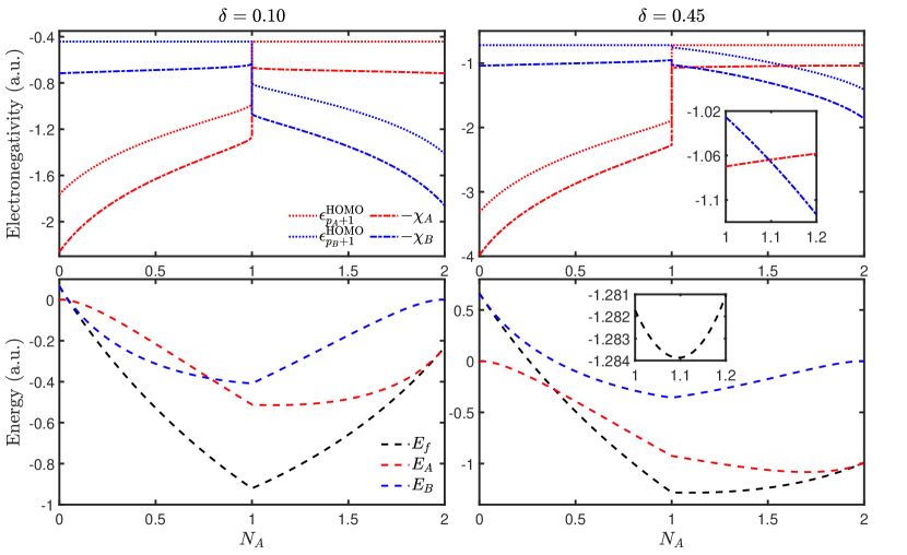
Figure 5: Top left: Negative electronegativities of fragments and HOMO energies as a function of $N_{A}$ for the two-electron molecule $\mathrm{AB^{+\delta}}$ of Sec.III-B ($Z_{A}=1.1$ and $Z_{B}=1$) with LDA and ENS at internuclear distance $R=1.446$ a.u.. $\epsilon_{M}^{\mathrm{HOMO}}=-0.4419$ a.u.. Bottom left: Fragment energies and their sum as a function of $N_{A}$. Top and bottom right panels are the same as top and bottom left, respectively, but with $Z_{A}=1.45$.

We begin by finding the optimum populations by identifying the value of $N_{A}$ at which the electronegativities of $A$ and $B$ become equal. Special care is needed here, however, as the ENS electronegativities are undefined at strictly integer populations, but one can define left- (right-) electronegativities, $\chi^{-}_{\alpha}$ ($\chi^{+}_{\alpha}$), as the left (right) limits of $-\frac{\partial\widetilde{E_{\alpha}}\left[n_{\alpha}\right]}{\partial n_{\alpha}\left(\mathbf{r}\right)}$. Figure 5 shows that fragment electronegativities are discontinuous at $N_{A}=1$. When $Z_{A}=1.1$, $N_{A}=1$ is the global minimizer of $E_{f}$. However, when $Z_{A}=1.45$, $N_{A}=1$ is no longer the global minimizer (the inset in the lower right panel of Fig.5 shows that $N_{A}^{*}=1.1$ leads to a slightly lower $E_{f}$ than $N_{A}=1.0$). How can one know if the global minimizer of $E_{f}$ will involve integer or fractional populations? Figure 6 provides the answer. The left and right electronegativites at $N_{A}=1$ are shown here as a function of $Z_{A}$. We find that when $1\leq Z_{A}\leq 1.422$, the intersection of $\left[-\chi_{A}^{-},-\chi_{A}^{+}\right]$ and $\left[-\chi_{B}^{+},-\chi_{B}^{-}\right]$ is not empty (shaded area in Fig.6), and $N_{A}=1$ is the global minimizer of $E_{f}$. Otherwise, $N_{A}=1$ is no longer the global minimizer of $E_{f}$, and the optimum populations become fractional, in agreement with the electronegativity equalization principle.

The FOO electronegativities are well defined when the electron populations are integers Janak (1978). There is no need to define left and right quantities here, as in ENS. The behavior of the $\chi_{\alpha}^{\rm FOO}$’s is similar to that of the one-electron electronegativites of Fig.(3).

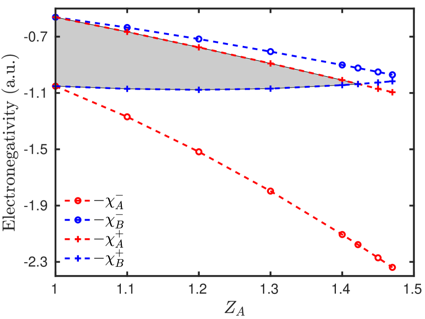
Figure 6: ENS-LDA left and right electronegativities of fragment A and B as a function of $Z_{A}$ for the two-electron model molecule $\mathrm{AB^{+\delta}}$ of Sec.III-B ($Z_{B}=1$) at internuclear distance $R=1.446$ a.u. when $N_{A}=N_{B}=1$. The shaded area corresponds to the range of $Z_{A}$ for which the optimum fragment populations are strictly integers.

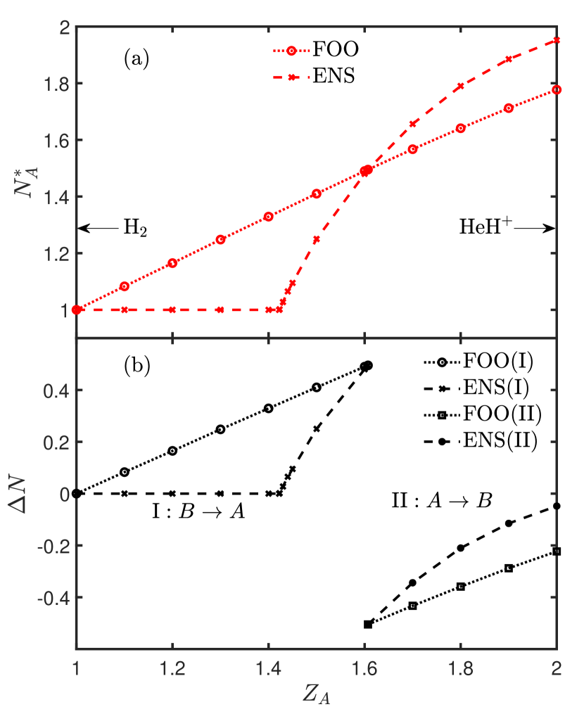
Figure 7: Top panel: Optimal electron population of fragment A, $N_{A}^{*}$, as a function of $Z_{A}$ for the two-electron model molecule $\mathrm{AB^{+\delta}}$ ($Z_{B}=1$) with FOO and ENS, at internuclear distance $R=1.446$ a.u. Bottom panel: The number of electrons transferred from fragment B to A, $\Delta N$, as a function of $Z_{A}$ for the two dissociation channels discussed in the text.

Figure 7 compares $N_{A}^{*}(Z_{A})$ from FOO and ENS. While the optimum numbers are non-integers in FOO for the entire range $1<Z_{A}\leq 2$, they are integers in ENS when $1<Z_{A}\leq 1.422$ for the reasons mentioned above. Figure 7 also shows that FOO and ENS yield the same $N_{A}^{*}$ at $Z_{A}=1.607$. This is the critical nuclear charge above which Channel II becomes the ground state. To emphasize this point, Figure 7 shows the number of electrons transferred $\Delta N$ for the range $1<Z_{A}<2$, indicating the ground-state dissociation channel in each case. Electrons are transferred from $B$ to $A$ when $Z_{A}<1.607$ and from $A$ to $B$ when $Z_{A}>1.607$. We note that $|\Delta N|$ is always lower in ENS than in FOO. The ENS fragment dipoles are also always smaller (Fig.8) .

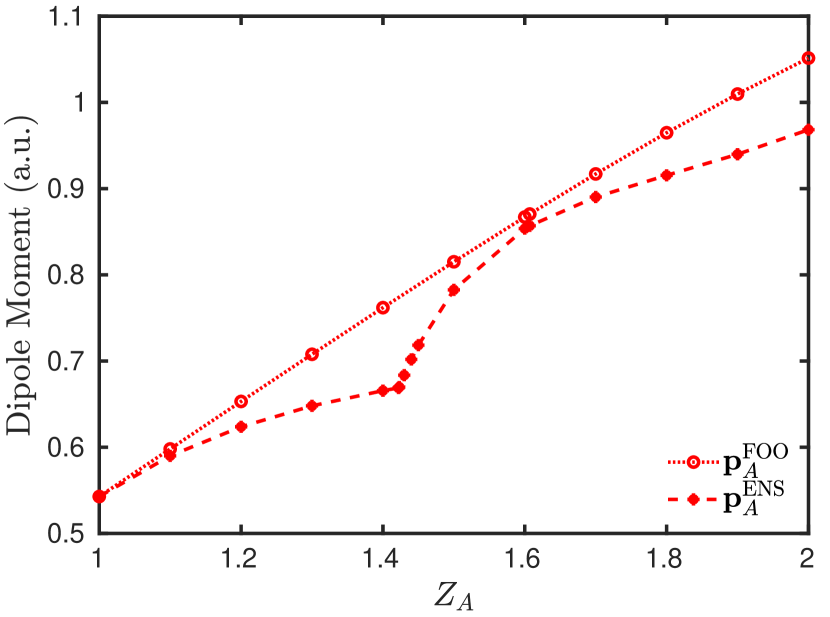
Figure 8: Electronic dipole moments of fragment A as a function of $Z_{A}$ for the two-electron model molecule $\mathrm{AB^{+\delta}}$ ($Z_{B}=1$) with FOO and ENS.

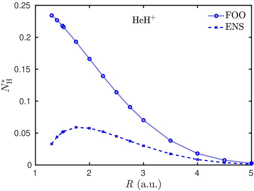
Figure 9: Optimal electron population of fragment H, $N_{\rm H}^{*}$, as a function of internuclear distance for $\mathrm{HeH}^{+}$ with FOO and ENS.

Dissociation of HeH⁺: We now compare FOO and ENS results for the optimum number of electrons transferred in HeH⁺ as the internuclear separation increases from $R\sim 1$ a.u. up to $R\sim 5$ a.u. (Figure 9). The separated state of $\mathrm{HeH}^{+}$ is a helium atom and a proton. The proton is dressed with a small fraction of an electron at finite $R$ and we note that the qualitative behavior of this small fraction $N_{\rm H}^{*}(R)$ is similar to that observed in the exact case for the 1-electron molecule of Sec.III-A (Figure 2): (1) The fraction of an electron reaches a maximum for ENS at $R\sim 1.8$ a.u.; (2) The FOO and ENS values approach each other as $R$ grows; and (3) The electron fraction given by FOO is larger than that given by ENS for all $R$.

III.3 Four electrons: Lithium hydride

Finally, we briefly examine the 4-electron molecule LiH at its equilibrium separation ($R_{eq}=3.03$ a.u.). In previous work Nafziger, Wu, and Wasserman (2011), it was speculated that the optimal P-DFT electron populations of the atomic fragments would be non-integers at $R_{eq}$. However, a recent exact P-DFT calculationOueis and Wasserman (2018) of a one-dimensional two-electron model of $\mathrm{LiH}$ yielded strictly integer populations. Figure 10 shows our LDA P-DFT energies for 3D $\mathrm{LiH}$ using both ENS and FOO. We find that, using ENS, the populations are indeed integers, as in the one-dimensional two-electron model Oueis and Wasserman (2018). Although the densities of $\mathrm{Li}$ and $\mathrm{H}$ fragments are distorted versions of the corresponding isolated-atom densities (see the H-atom density distortions in Fig.11), there is no electron transfer between fragments in ENS. However, using FOO, the fragment electron populations are non-integral. At the equilibrium internuclear distance, $R_{eq}=3.03$ a.u., we obtain $N_{\mathrm{Li}}^{*}=2.663$ and $N_{\mathrm{H}}^{*}=1.337$. The number of electrons transferred from $\mathrm{Li}$ to $\mathrm{H}$ is $\Delta N=0.337$. Just as in the examples of Secs.III-A and III-B, the number of electrons transferred with the FOO method is larger than with the ENS method (which is just zero in this case). To understand why, we distinguish three zones and note that when the number of electrons in the lithium atom is less than the optimum predicted by FOO (zone 1: $N_{\mathrm{Li}}<2.663$) then $\epsilon_{\mathrm{H},\mathrm{FOO}}^{\mathrm{HOMO}}=\epsilon_{\mathrm{H},\mathrm{ENS}}^{\mathrm{HOMO}}=\epsilon_{\mathrm{LiH}}^{\mathrm{HOMO}}$. However, when that number is higher than the optimum predicted by ENS (zone 2: $N_{\mathrm{Li}}>3.0$) then $\epsilon_{\mathrm{Li},\mathrm{FOO}}^{\mathrm{HOMO}}=\epsilon_{\mathrm{Li},\mathrm{ENS}}^{\mathrm{HOMO}}=\epsilon_{\mathrm{LiH}}^{\mathrm{HOMO}}$. Finally, when $N_{\mathrm{Li}}$ is in between those two values (zone 3: $2.663<N_{\mathrm{Li}}<3.0$) then $\epsilon_{\mathrm{Li},\mathrm{FOO}}^{\mathrm{HOMO}}=\epsilon_{\mathrm{H},\mathrm{ENS}}^{\mathrm{HOMO}}=\epsilon_{\mathrm{LiH}}^{\mathrm{HOMO}}$ and $\epsilon_{\mathrm{Li},\mathrm{ENS}}^{\mathrm{HOMO}}<\epsilon_{\mathrm{LiH}}^{\mathrm{HOMO}}$. Our analysis of Sec.II-C then implies that $v_{p}^{\mathrm{ENS}}\left(\mathbf{r}\right)$ is deeper than $v_{p}^{\mathrm{FOO}}\left(\mathbf{r}\right)$ (Fig.12) and $E_{f}^{\mathrm{ENS}}>E_{f}^{\mathrm{FOO}}$ (Fig.10). It can be seen in Fig.12 that the partition potential does not change qualitatively when $N_{\mathrm{Li}}$ crosses from zone 1 to zone 3, but there are major qualitative changes when it crosses to zone 2.

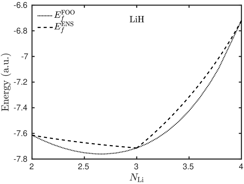
Figure 10: The sum of fragment energies, $E_{f}$, as a function of $N_{A}$ for $\mathrm{LiH}$ with FOO and ENS at the equilibrium internuclear distance $R=3.03$ a.u.

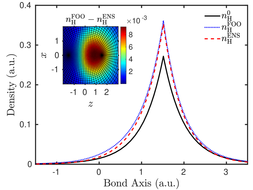
Figure 11: Optimal electron densities for the $\mathrm{H}$ fragment in $\mathrm{LiH}$ with FOO and ENS at the equilibrium internuclear distance $R=3.03$ a.u.; the solid line corresponds to an isolated hydrogen atom density. The inset shows the difference between the FOO and ENS fragment densities on the $xz$-plane.

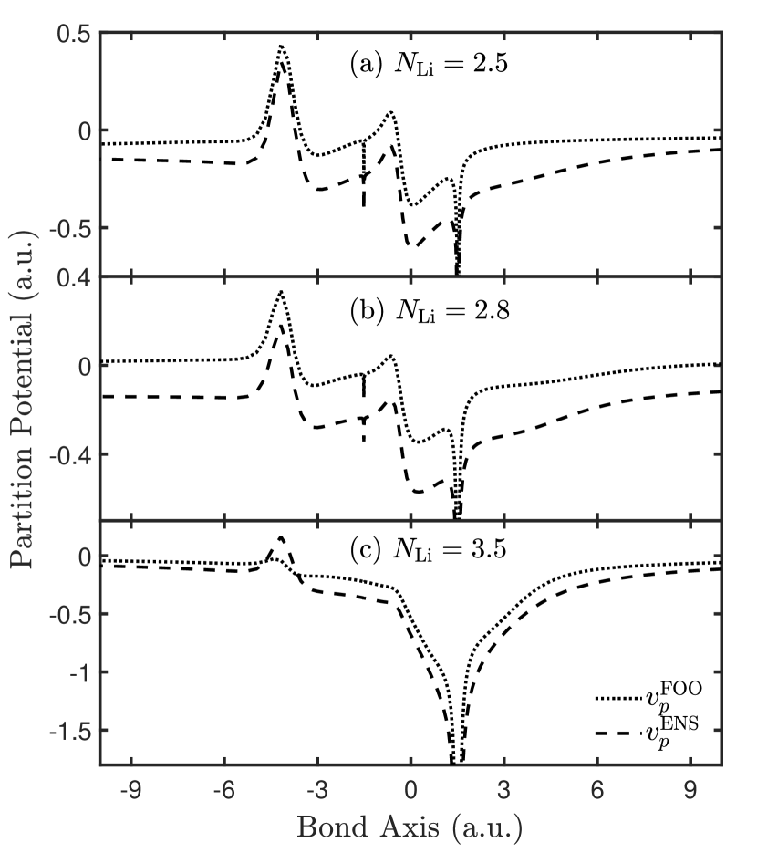
Figure 12: Partition potential along the bond axis for $\mathrm{LiH}$ with FOO and ENS at the equilibrium internuclear distance $R=3.03$ a.u. when $N_{\mathrm{Li}}=$ (a) 2.5, (b) 2.8, and (c) 3.5.

IV Concluding remarks

By treating fragment electron populations as variables in P-DFT calculations, we have shown how to find optimal populations via two alternative methods, one that involves fractional orbital occupations (FOO), and another that makes use of ensemble averages (ENS). The optimal populations are found in both cases when the sum of fragment energies $E_{f}$ reaches its global minimum and all fragment electronegativities become equal. At that optimum, a value for the charge transferred between two fragments can be assigned unambiguously even at finite internuclear separations.

Through the formal analysis of Sec.II and the explicit numerical calculations of Sec.III, we have revealed differences between FOO and ENS that had not been observed in previous studies: (1) Although both methods lead to the same molecular densities and energies, the fragment densities of hetero-nuclear diatomic molecules can be significantly different, with the FOO method consistently yielding a larger fraction of an electron transferred from donor to acceptor, at least when the LDA is employed; (2) The FOO fragment dipole moments are observed to provide an upper bound to the corresponding ENS dipole moments; (3) The ENS partition potentials are deeper than the corresponding FOO partition potentials; (4) Accordingly, $E_{f}^{\mathrm{ENS}}>E_{f}^{\mathrm{FOO}}$ and $E_{p}^{\mathrm{ENS}}<E_{p}^{\mathrm{FOO}}$.

Although a general proof of these observations is far beyond the scope of the present work, we suspect that FOO will generally transfer more electrons than ENS: When the nuclei are far enough apart, the effect of the partition potential on the fragment densities is negligible and the ENS fragment energies vary linearly with electron number. Since this occurs for both fragments, and since the FOO energies are observed to be convex functions of the electron number, the sum of fragment energies is expected to be lower in FOO than in ENS. The situation is less clear at finite internuclear separations $R$, but the small deviations from linearity detected for ENS even at small $R$ (certainly at equilibrium), suggest that the conclusions will remain valid in general at finite $R$.

With appropriate approximations to the partition energy functional, P-DFT has been recently shown to overcome static-correlation and delocalization errors when stretching homonuclear diatomic molecules Nafziger and Wasserman (2015). Also for homonuclear diatomic molecules, a proposed “covalent" approximation for the non-additive non-interacting kinetic energy shows promising results for orbital-free calculations Jiang, Nafziger, and Wasserman (2018). An extension of these approximations to the ionic case and, more generally, to chemical bonds connecting inequivalent fragments, would be desirable. This extension will require choosing a method to treat fractional populations. Although both FOO and ENS methods are valid candidates, the results of this work point to advantages of each method in different cases: The observation that ENS fragment densities are less distorted than FOO densities upon formation of a chemical bond is a significant advantage for ENS, both conceptually and computationally. Conceptually, it is pleasing to have fragments-in-molecules that are minimally distorted from their isolated counterparts. Computationally, although each iteration of the P-DFT equations involves two integer-number calculations (vs. only one in FOO), the minimal distortion of the isolated input densities leads to a faster convergence that will benefit future applications. On the other hand, the FOO method has an advantage over ENS at equilibrium separations, as fractional populations are more in line with the chemist’s intuition that polar molecules are composed of fragments with fractional formal charges.