Scaling limits of Maximal Entropy Random Walks on a non-negative integer lattice perturbed at the origin

 

Abstract We investigate random walks on the integer lattice perturbed at the origin which maximize the entropy along the path or equivalently the entropy rate. Compared to usual simple random walks which maximize the entropy locally, those are a complete paradigm shift. For finite graph, they have been introduced as such by Physicists in [BDLW09] and they enjoy strong localization properties in heterogeneous environments. We first give an extended definition of such random walks when the graph is infinite. They are not always uniquely defined contrary to the finite situation. Then we introduce our model and we show there is a phase transition phenomenon according with the magnitude of the perturbation. We obtain either Bessel-like or asymmetric random walks and we study there scaling limits. In the subcritical situation, we get the classical three-dimensional Bessel process whereas in the supercritical one we get a recurrent reflected drifted Brownian motion. We produce a unify proof relying on the equivalence between submartingale problems and reflected stochastic differential equations obtained in [KR17]. Finally, we remark that applying our results to a couple of particles subject to the famous Pauli exclusion principle, we can recover the electrostatic force assuming only the maximal entropy principle. Also, we briefly explain how to retrieve those results in the macroscopic situation without go through the microscopic one by using the Kullback–Leibler divergence and the Girsanov theorem.

 

Key words  Random walks . Maximum entropy principle . Functional scaling limits . Reflected diffusions . Submartinagle problem

Mathematics Subject Classification (2000)  60G50 . 60F17 . 60G42 . 60G44 . 60J10 . 60J60 . 60K99 . 60C05 . 82B41 . 82B26 . 05C38 . 05A15 . 94A17

1 Introduction

The most popular way to randomly explore a given locally finite graph $G$, without any further information, is to assume that the walker sitting at a node of out degree $k$ jumps onto any neighboring node with uniform probability $1/k$, and that independently at every time .This Markov process is called a Generic Random Walk (GRW) and this choice among all the random walks we can consider is that maximizing the entropy production at each step.

The concept of entropy introduced by Ludwig Boltzmann 1870s is fundamental in the fields of Statistical Physics and Thermodynamics but also in the field of Information Theory developed by Claude Shannon in the 1940s. We refer to their groundbreaking papers [SM15, Sha48]. Here, all we need to known is that the entropy of a distribution $\mu$ on a countable set $E$ is defined by

$$H(\mu)=-\sum_{x\in E}\mu(x)\ln(\mu(x))\in[0,\infty].$$ (1.1)

When $X$ is a random variable on $E$, the quantity $H(X)$ has to be understood as the entropy of the distribution of $X$. Besides, if $N={\rm card}(E)$ is finite, the maximum of $H(\mu)$ is achieved when $\mu$ is the uniform probability measure on $E$ and it is equal to $\ln(N)$. Regarding the Markov chain theory on a countable state space $E$, a quantity of particular interest is the entropy rate

$$h=\lim_{n\to\infty}\frac{H(X_{0},\cdots,X_{n})}{n}=\lim_{n\to\infty}\frac{1}{n}\sum_{c\in\mathcal{C}_{n}}\mu_{n}(c)\ln(\mu_{n}(c)),$$ (1.2)

where $\mu_{n}$ denotes the distribution of the Markov chain trajectory $(X_{0},\cdots,X_{n})\in\mathcal{C}_{n}$. When the latter is irreducible and positive recurrent, $h$ does not depend on the distribution of $X_{0}$ and it can be written from its invariant probability measure $\pi$ and its transition kernel $(p(x,y))_{x,y\in E}$ as

$$h=-\sum_{x,y\in E}\pi(x)p(x,y)\ln(p(x,y)).$$ (1.3)

When the stochastic process is stationary, that is when $X_{0}$ is distributed as $\pi$, it has to be noted that the sequence in the right-hand-side of (1.2) is constant. Concerning Markov chain and entropy we refer to [Khi57, EC93] for instance. Besides, since for an irreducible GRW on a finite lattice, the probability of finding the particle at node $x$ is proportional to the outer degree $d(x)$ in the stationary state, it comes

$$h_{GRW}=\frac{\sum_{x\in E}d(x)\ln(d(x))}{\sum_{x\in E}d(x)}.$$ (1.4)

The Maximum Entropy Random Walks (MERWs) are somehow a paradigm shift, from local to global. Roughly speaking, we are looking for irreducible random walks on a graph maximizing the path entropy or, equivalently, the entropy rate. This formulation has been introduced recently in [Dud12, BDLW10, BDLW09]. Among others results, the authors highlight strong localization phenomenon of MERWs for slightly disordered environments, which is particularly relevant in Quantum Mechanics when we study the phenomenon of Anderson localization. We refer for instance to [K1̈6] for a mathematical survey. Also, this notion of MERW is very close to that of Parry measure for sub-shifts of finite type defined in [Par64]. Also, it has a hand with the iteration of matrices, it appears between the lines in [Het84, AGD94], and it could be useful to study complex networks as in [SGGnL⁺11, DL11, DM05].

Indeed, when the graph is finite and irreducible, the Perron-Frobenius theorem insures that such random walk exists and is unique. Its Markov kernel and invariant probability measure is given by

$$p(x,y)=A(x,y)\frac{\psi(y)}{\rho\psi(x)}\quad\mbox{and}\quad\pi(x)=\psi^{2}(x),$$ (1.5)

where $A$ is the adjacency matrix of $G$, $\rho$ its spectral radius and $\psi$ the associated $\ell^{2}(G)$-normalized positive eigenfunction. In that case the entropy rate is nothing but $h_{MERW}=\ln(\rho)$. Surprisingly, or not, all the trajectories of length $n$ between two given points $x$ and $y$ are of the probability given by $\psi(y)/\rho^{n}\psi(x)$. Even if the path distributions are not uniform, conditionally on the their length and the extreme stated they are. Hence we can glimpse all the combinatorial features that can result from MERWs. Besides, the kernel in (1.5) reminds the well-known Doob $h$-transform appearing in particular when stochastic processes are conditioned to stay in a given domain. We can refer to [Doo01] and [KS10].

The positive eigenfunction $\psi$ is well-known when we classify the influence of nodes in complex networks, it is used in the eigenvector centrality (see [ASGD] for instance). For the Physicists, it can be viewed as a wave function and, more precisely, it is the ground state of a discrete Schrödinger equation whose potential $V$ is given by the opposite of the degree, that is

$$-\Delta\psi(x)+V(x)\psi(x)=-\rho\,\psi(x),$$ (1.6)

where $\Delta$ is the discrete Laplacian on the graph and $V(x)=-\sum_{y\in G}A(x,y)$. One can easily generalized such construction replacing the adjacency matrix by a weighted one and we can even add some energetic constrains as it is explained in [Dix15]. However, the mathematical framework of MERW has to be inquired further and a lot remains to be done.

To begin with, there is stil few solvable models in which the spectral radius and the associated wave function are explicit. We allude to [OB12] dealing with Cayley trees for instance. Of course, when the graph size is small enough, one can compute them numerically in order to make computer simulations of the MERW but it is not always the case. Furthermore, and it is the main topic of this paper, in the case of infinite lattices, there is no consistent results as far as our knowledge. An infinite periodic lattice is mentioned in [BDLW10] and some diffusion coefficient is compute but many questions had not been raised yet.

• What could be the right definition of the MERW in an infinite lattice ?

• Is there existence and uniqueness of such MERW ?

• What can be said about scaling limits of MERWs compared with those for GRWs ?

One of our purpose is to show that many classical continuous-time processes can be reinterpreted as scaling limits of some MERW. The scaling limits archetype are the famous Donsker’s results, initiated in [Don51], which gave rise to a fruitful literature helping us to understand how we go from some microscopic states to macroscopic ones. Originally, Donsker’s Theorem states under suitable assumptions that scaling limits of GRWs lead to Brownian motions.

Outline of the article  In this paper we define MERWs on some general infinite lattice in section 2.1. Then we consider our model in section 2.2 : the natural number lattice $\mathbb{N}_{0}=\{0,1,2,\cdots\}$ perturbed at the origin with some weight $\gamma\geq 0$. We refer to Figure 1. We highlight a phase transition phenomenon on the spectral radius and we show in 2.3 when $\gamma=0$ that the MERW can be viewed as a the usual random walk conditioned to stay positive. In section 2.4 we state the functional scaling limits we obtain. When $\gamma=1$ the limit stochastic process is the standard reflected Brownian motion whereas when $0\leq\gamma<1$ it is the celebrated three-dimensional Bessel process (2.25). It can be viewed as a Brownian motion conditioned to stay positive and it can be obtain by a Doob $h$-transform of the Brownian motion. We can allude to [Wil74, Pit75] and to [Lam62, Ale11] regarding Bessel-like random walks. Those Markov processes are transient and thus we say that the origin is repulsive in the subcritical case. In the supercritical situation, when $\gamma=1+\lambda/\sqrt{n}$, we obtain the ergodic reflected diffusion (2.26). As an application, we study a pair of particle in subject to the Pauli exclusion principle and the maximal entropy principle. We can interpret the electrostatic repulsion as an entropic force as in [Wan10]. We point out that such questions are raised in [Dud12]. Furthermore, we explain in the much more tedious situation of continuous-time stochastic processes how it is possible to directly interpret the latter diffusions as those which maximize some pathwise entropy. Finally, we prove the functional scaling limits in section 3.

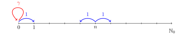
Figure 1: The model

2 Results

2.1 General framework

In order to introduced the MERWs we investigate, we begin with defined the spectral radius analogue to the finite situation. We refer to [VJ67] for more details about infinite positive matrix and especially to Theorem B, p. 364.

Definition 2.1 (Combinatorial spectral radius).

Let $A$ be the weighted adjacency matrix of a (possibly infinite) irreducible weighted graph $\mathcal{G}$ such that $V(x)=\sum_{y\in G}A(x,y)$ is uniformly bounded. Let $x,y$ be any state in $G$. The combinatorial spectral radius $\rho$ is the inverse of the positive radius of convergence of the resolvent $\sum_{n=0}^{\infty}A^{n}(x,y)\,z^{n}$ It does not depend on $x,y$.

Roughly speaking, the combinatorial spectral radius $\rho$ means that the leading asymptotic of the weighted-number of $n$-step trajectories from $x$ to $y$ is of order $\rho^{n}$.

Definition 2.2 (MERW).

Let $G$ be a graph satisfying the assumptions of Definition 2.1 with the same notations. A MERW on $G$ is any random walk whose transition probabilities can be write as

$$p(x,y)=A(x,y)\frac{\psi(y)}{\rho\,\psi(x)},$$ (2.7)

where $\psi$ a positive eigenvector of $A$ associated with $\rho$. There exists at least one MERW.

We have to note that contrary to the finite situation, there exist a unique or an infinity of MERWs. A simple example can be explained when $G=\mathbb{Z}$ with the usual nearest neighbors relations $A(x,x\pm 1)=1$ for every $x\in\mathbb{Z}$ and the loops $A(x,x)=1$ excepted when $x=0$. In that case it can showned that $\rho=3$ and $\psi_{+}(x)=1+x\mathds{1}_{\{x\geq 0\}}$ and $\psi_{-}(x)=\psi_{+}(-x)$ are two positive eigenfunctions. As a matter of facts, any positive eigenfunction with $\psi(0)=1$ can be written as a convex combination $\lambda\psi_{+}+(1-\lambda)\psi_{-}$ with $0\leq\lambda\leq 1$. The eigenfunctions $\psi_{\pm}$ are extremal. This is close to the theory of positive harmonic functions and the Martin or Poisson boundary. See for instance [Doo01]. However, one a sufficient criterion for the uniqueness which can be found again in [VJ67].

Proposition 2.1 ($R$-recurrence).

With the same assumptions on $G$ as in the latter definitions, if $A$ is $R$-recurrent, that is when $\sum_{n\geq 0}A^{n}(x,y)\rho^{-n}=\infty$ for any or some $x,y\in G$, then there exists a unique MERW. In this case, it is positive-recurrent.

2.2 The model

Let $\gamma\geq 0$ be and consider the nearest neighborhood weighted lattice on $\mathbb{N}_{0}$ given by the weighted adjacency matrix $A$ defined by $A_{0,0}=\gamma$, $A_{0,1}=1$ and $A_{n,n\pm 1}=1$ for every $n\geq 1$. When $\gamma=1$ the graph is regular since every vertex is of degree 2. Otherwise, the degree of the origin is less or greater than $2$. The latter can be called repulsive or attractive as we shall explain in the sequel. We first note there is a phase transition phenomenon regarding the combinatorial spectral radius.

Proposition 2.2.

The combinatorial spectral radius satisfies

$$\rho=\left\{\begin{array}[]{lll}2,&\mbox{if}&{\gamma}\leq 1.\\ {\gamma}+\frac{1}{{\gamma}},&\mbox{if}&{\gamma}\geq 1.\end{array}\right.$$ (2.8)

Proof.

First assume that $0\leq\gamma\leq 1$. One has $C_{n}\leq A^{2n}_{0,0}\leq 4^{n}$ where $C_{n}$ is the $n$-th Catalan number. Note that $A^{n}_{0,0}$ as soon as $n$ is an odd number. Since $C_{n}\sim\pi^{-1/2}n^{-3/2}4^{n}$, we obtain that $\rho=2$. Finally, assume that $\gamma>1$. Set $a_{n}=A^{n}_{0,0}$ and thereafter

$$G(z)=\sum_{n=0}^{\infty}a_{n}z^{n}\quad\mbox{and}\quad S(z)=\sum_{n=0}^{\infty}C_{n}z^{2n}=\frac{1-\sqrt{1-4z^{2}}}{2z^{2}}.$$ (2.9)

Let $R=1/\rho$ be the radius of convergence of $G$ Following the powerful methods of algebraic-combinatorics, illustrated in particular in [Fla80, Ban01, BF02] for instance, one has

$$G(z)=\frac{1}{1-\gamma z-z^{2}S(z)},$$ (2.10)

for any $|z|<R$. One can see that these two terms are equal as formal power series to

$$\sum_{k\in\mathbb{N}}\;\sum_{\stackrel{{\scriptstyle n_{-1},n_{0},n_{1}\cdots}}{{\sum_{i=-1}^{\infty}n_{i}=k}}}\binom{k}{n_{-1},n_{0},n_{1},\cdots}\gamma^{n_{-1}}\left(\prod_{i=0}^{\infty}a_{i}^{n_{i}}\right)z^{n_{-1}+\sum_{i=0}^{\infty}n_{i}(i+2)}.$$ (2.11)

Indeed, it follows directly from the power series expansion of $(1-X)^{-1}$ and the multinomial theorem that the right-hand-side of (2.10) is equal to (2.11). Concerning the left-hand-side, we can describe any trajectory from $0$ to $0$ with some numbers $n_{0},n_{1},\cdots$ of trajectories into $\{1,2,\cdots\}$, whose respective length are $0,1,\cdots$, starting and ending to $1$, after the walker moves from $0$ to $1$ and followed by a return to $0$. To complete the description, we also need to count the number $n_{-1}$ of times the edge $(0,0)$ is taken. The length of the trajectory is nothing but than $n_{-1}+\sum_{i\geq 0}n_{i}(i+2)$ whereas $k=n_{-1}+n_{0}+n_{1}+\cdots$ is the number of sub-trajectories in the decomposition which can rearrange as many times as the multinomial coefficient in the later expression does.

In particular, since all the coefficients involved are non-negative, the power series (2.11) is absolutely convergent on $[0,R[$ as $G$ but also, as the right-hand side of (2.10), on $[0,x_{\ast}[$ where $x_{\ast}$ is the maximal positive number for which $0\leq\gamma x+x^{2}S(x)<1$. One can easily check that $x_{\ast}={\left(\gamma+{1}/{\gamma}\right)}^{-1}$. It is then straightforward to see that $R=x_{\ast}$ and thus $\rho=\gamma+{1}/{\gamma}$. ∎

Proposition 2.3.

Given $\gamma\geq 0$ there exists a unique MERW on the non-negative integer. Let $P$ be its probability transitions.

1. If $\gamma<1$ then

   $$P_{n,n+1}=\frac{1}{2}\frac{2-\gamma+(1-\gamma)n}{1+(1-\gamma)n},\quad P_{n,n-1}=\frac{1}{2}\frac{\gamma+(1-\gamma)n}{1+(1-\gamma)n}\quad\mbox{and}\quad P_{0,0}=\frac{\gamma}{2}.$$ (2.12)

   Here $n,n+1,n-1$ belong to $\mathbb{N}_{0}$. Besides, the MERW is transient and $\pi_{n}=(1+(1-\gamma)n)^{2}$ is an invariant measure for this Markov chain.

2. If $\gamma=1$ then the transition probabilities are still given by (2.12) and thus $P_{n,n+1}=1/2$ and $P_{n,n-1}=1/2$ for every $n\geq 1$ and $P_{0,0}=1/2$. It is null-recurrent and its invariant measure is up to some multiplicative constant the counting measure on $\mathbb{N}_{0}$.

3. If $\gamma>1$ then

   $$P_{n,n+1}=\frac{1}{1+\gamma^{2}},\quad P_{n,n-1}=\frac{\gamma^{2}}{1+\gamma^{2}}\quad\mbox{and}\quad P_{0,0}=\frac{\gamma^{2}}{1+\gamma^{2}}.$$ (2.13)

   Furthermore, the MERW is positive recurrent and its invariant probability measure is given by the geometric distribution on $\mathbb{N}_{0}$ of parameter $1-1/\gamma^{2}$, that is

   $$\pi_{n}=\frac{1}{\gamma^{2n}}\left(1-\frac{1}{\gamma^{2}}\right).$$ (2.14)

Remark 2.1.

When $0\leq\gamma<1$ the MERW is a particular case Bessel-like random walk as they are defined in [Ale11].

Proof.

We are looking for solutions $\psi:\mathbb{N}_{0}\longrightarrow(0,\infty)$ of

$$\left\{\begin{array}[]{l}\psi_{n+1}+\psi_{n-1}=\rho\,\psi_{n},\;n>0.\\ \psi_{1}+\gamma\psi_{0}=\rho\,\psi_{0}.\end{array}\right.$$ (2.15)

It follows from the boundary conditions that $\psi_{0}$ being fixed, say for instance $\psi_{0}=1$, $\psi_{1}$ is uniquely defined as all the $\psi_{n}$, $n\in\mathbb{N}_{0}$. This proves the uniqueness of the associated MERW. If $\gamma\leq 1$, it suffices to solved the characteristic polynomial $X^{2}-\rho X+1=0$ and to used the boundary condition to get the latter expressions. When $\gamma>1$, the same method applies but it is more tedious. Solving the characteristic polynomial $X^{2}-(\gamma+{1}/{\gamma})X+1=0$ we get that any solution takes the form

$$\psi_{n}=\lambda\,\gamma^{n}+\mu\,\frac{1}{\gamma^{n}}.$$ (2.16)

Since $\psi_{1}=(1/\gamma)\psi_{0}$ it comes that $\lambda=0$ and this leads to (2.13).

Regarding the recurrence or transience properties, we begin with $\gamma=0$. Recall that $A_{0,0}^{2n}=C_{n}$ is the $n$-th Catalan number. It follows that the corresponding MERW is transient since

$$\sum_{n\geq 0}P_{0,0}^{n}=\sum_{n\geq 0}\frac{C_{n}}{4^{n}}<\infty.$$ (2.17)

More generally, when $\gamma<1$, we use the generating function $G$ in (2.9). As previously, one can check that $G$ satisfies (2.10) on $[0,1/2]$. Since $A_{0,0}^{2n}\geq C_{n}$ the radius of convergence $R$ of $G$ is equal to $1/2$ and we obtain

$$G(1/2)=\sum_{n\geq 0}P_{0,0}^{n}=\frac{2}{1-\gamma}<\infty.$$ (2.18)

Similarly, when $\gamma=1$, $G(1/2)=\infty$ and we deduce the recurrence of the MERW. The latter is null recurrent since the invariant measure is $\psi_{i}^{2}=(1+i)^{2}$. When $\gamma>1$ one has $\psi_{i}^{2}={\gamma^{-2i}}$ and this completes the proof. ∎

2.3 A random walk conditioned to stay positive

Proposition 2.4.

Let $\{S_{n}\}_{n\geq 0}$ be the simple symmetric random walk on $\mathbb{Z}$. Then the distribution of $S$ conditioned to stay in $\mathbb{N}_{0}$ is the MERW when $\gamma=0$.

Remark 2.2.

It is well-known that a Brownian conditioned to stay positve is nothing but a three-dimensional Bessel process (see [Pit75]) for instance). Furthermore, functional scaling limits of random walks conditioned to stay positive have also been investigated since [Igl74, Bol76] and lead to the same limit under suitable assumptions. Even if Proposition (2.4) must be well-known, we do not find any reference and we present an elementary proof.

Proof.

Let us introduce $\tau=\inf(\{n\geq 0:S_{n}=-1\})$. One has

$$\mathbb{P}_{x}(\tau=n)=\frac{x+1}{n}\mathbb{P}_{0}(S_{n}=x+1).$$ (2.19)

Indeed, we first write

$$\mathbb{P}_{x}(S_{1}>-1,\cdots,S_{n-2}>-1,S_{n-1}=0,S_{n}=-1)=\\ \frac{\mathbb{P}_{0}(S_{n-1}=x)-\mathbb{P}_{0}(S_{n-1}=x,\exists\,0\leq k\leq n-1\,\,S_{k}=x+1)}{2}.$$ (2.20)

Then applying the reflexion principle, we get

$$\mathbb{P}_{x}(\tau=n)=\frac{\mathbb{P}_{0}(S_{n-1}=x)-\mathbb{P}_{0}(S_{n-1}=x+2)}{2}.$$ (2.21)

Besides, one can check that

$$\mathbb{P}_{0}(S_{n}=y)=\frac{1}{2^{n}}\binom{n}{\frac{n+y}{2}}\underset{n\to\infty}{\sim}\frac{1}{\sqrt{\pi n}},$$ (2.22)

when $n+y\in 2\mathbb{Z}$ and $0\leq n+y\leq 2n$. Furthermore, we deduce from the latter asymptotic that

$$\mathbb{P}_{x}(\tau>n)\sim\frac{2(x+1)}{\sqrt{\pi n}}.$$ (2.23)

Finally, given any path $x\to x_{1}\to\cdots\to x_{k-1}\to y$ into $\mathbb{N}_{0}$, one can write

$$\mathbb{P}_{x}(S_{1}=x_{1},\cdots,S_{k-1}=x_{k-1},S_{k}=y|\tau>n)\\ =\mathbb{P}_{x}(S_{1}=x_{1},\cdots,S_{k-1}=x_{k-1},S_{k}=y)\frac{\mathbb{P}_{y}(\tau>n-k)}{\mathbb{P}_{x}(\tau>n)}\\ \underset{n\to\infty}{\sim}\frac{1}{2^{k}}\frac{y+1}{x+1}.\hskip 256.0748pt$$ (2.24)

∎

2.4 Functional scaling limits

Before introduce our main result, we need to introduce some continuous-time stochastic processes involved in the scaling limits and we briefly recall some elementary settings about functional convergence in distribution.

In the sequel, let $x\in[0,\infty[$ be fixed and denote by $\{B_{t}\}_{t\geq 0}$ a one dimensional standard Brownian motion. Also, we introduce a three-dimensional Bessel process $\{Y_{t}\}_{t\geq 0}$ starting at $x$. We recall that $Y$ takes its values in $[0,\infty[$ and satisfies the stochastic differential equation

$$dY_{t}=dB_{t}+\frac{1}{Y_{t}}dt,\quad Y_{0}=x.$$ (2.25)

For these two stochastic processes and much more we refer to [RY99]. Note that $Y$ is transient and has for invariant measure $m(dx)=x^{2}dx$ on $[0,\infty[$. Also, we consider $W_{t}=|x+B_{t}|$ the reflecting Brownian motion starting from $x$. Finally, let $\lambda>0$ fixed and let $\{(Z_{t},L_{t})\}_{t\geq 0}$ be the solution of the following reflected stochastic differential equation

$$\left\{\begin{array}[]{l}dZ_{t}=dB_{t}-\lambda dt+dL_{t},\\ Z_{0}=x\\ Z_{t}\geq 0\\ \end{array}\right.$$ (2.26)

Here $L_{t}$ is a $B_{t}$-measurable non-decreasing stochastic process such that $L_{0}=0$ and

$$\int_{0}^{\infty}\mathds{1}_{\{Z_{t}>0\}}dL_{t}=0\quad\mbox{a.s.}.$$ (2.27)

It is classical that such solution exists and is unique, one can refer to [Tan79] or [C9́8] for a more general setting. Besides, one can check that $Z$ is a strong Markov process which is positive recurrent and whose invariant probability distribution is the exponential distribution of parameter $2\lambda$.

Finally, we endowed the space $\mathbb{D}$ of càdlàg real function on $[0,\infty)$ with the topology of uniform convergence on compact sets. In the sequel, we denote by $\Longrightarrow$ the convergence in distribution of stochastic processes in $\mathbb{D}$ with the associated Borel $\sigma$-field. We refer to [Bil99] or [Whi02] for a more extensive survey on functional convergences in distribution.

Theorem 2.1.

Let $\{X_{k}\}_{k\geq 0}$ be the MERW given in (2.3). Assume $X_{0}=x_{0}^{n}$ is deterministic and depends on $n$ in such way

$$\frac{x_{0}^{n}}{\sqrt{n}}\;\xrightarrow[n\to\infty]{}\;x.$$ (2.28)

Then, one has the following functional scaling limits.

1. If $\gamma<1$ then

   $$\left\{\frac{X_{\lfloor nt\rfloor}}{\sqrt{n}}\right\}_{t\geq 0}\;\ext@arrow 0359\Rightarrowfill@{n\to\infty}{}\;\{Y_{t}\}_{t\geq 0}.$$ (2.29)

2. If $\gamma=1$ then

   $$\left\{\frac{X_{\lfloor nt\rfloor}}{\sqrt{n}}\right\}_{t\geq 0}\;\ext@arrow 0359\Rightarrowfill@{n\to\infty}{}\;\{W_{t}\}_{t\geq 0}.$$ (2.30)

3. If $\gamma:=1+\frac{\lambda}{\sqrt{n}}$ then

   $$\left\{\frac{X_{\lfloor nt\rfloor}}{\sqrt{n}}\right\}_{t\geq 0}\;\ext@arrow 0359\Rightarrowfill@{n\to\infty}{}\;\{Z_{t}\}_{t\geq 0}.$$ (2.31)

Remark 2.3.

Since the increments of $\{X_{k}\}_{k\geq 0}$ are bounded, the same results hold replacing the stepwise constant stochastic processes by there continuous-times interpolations.

Remark 2.4.

When $0\leq\gamma<1$ this result can be obtained by using [Lam62]. However, we choose to present a more modern proof which relies on submartingale problems and which can be naturally extended to the critical situations when $\gamma=1$ or $\gamma=1+\lambda/\sqrt{n}$.

2.5 Application to some exclusion process

Let us consider the following two-bodies problem. We consider two particles on the integers we can only jump to the right or the left but which can not occupy the same site. This is the lattice structure of the usual exclusion process on the integers with only two particles. We refer to [Der98, Sch01] for reviews on this subject.

By symmetry, $\Psi(x,y)=1+(y-x)$ is clearly a positive eigenfunction of the exclusion lattice associated with the combinatorial spectral radius $\rho=4$. Here $x$ denotes the position of the first particle and $y$ the position of the second one and we suppose $x<y$. Such $\Psi$ is not necessarily unique, as the example below Definition 2.2 shows, but if we assume only jumps in one direction (the totally asymmetric situation) the latter is unique and it is then associated to the spectral radius $\rho=2$. Anyway, we get in the scaling limit

$$d(Y_{t}-X_{t})=dB_{t}+\frac{dt}{Y_{t}-X_{t}},$$ (2.32)

where $X_{t}<Y_{t}$ denote the position of the particles at time $t$. Here the interesting point is we make appeared the usual electrostatic force assuming only the maximal entropy constrain.

2.6 Continuous-time counterpart of MERW

In the light of these scaling limits, we can ask whether the three-dimensional Bessel process, the reflected Brownian motion or the reflected drifted Brownian motion can be interpreted as maximal entropy stochastic processes without the intermediate of MERWs.

To go further, the distribution $\gamma_{n}$ of the first $n$-steps of the MERW when $\gamma=1$ is uniform since the latter is nothing but than a simple random walk on a regular graph. As a product, maximize the entropy in the right-hand side of (1.2) is equivalent to minimize the Kullback–Leibler divergence (also known as the relative entropy) $D_{\rm KL}(\mu_{n}||\gamma_{n})$. We recall that given two probability measures $\mu,\gamma$ such that $\mu$ is absolutely continuous with respect to $\gamma$,

$$D_{\rm KL}(\mu\|\gamma)=\int\ln\left(\frac{d\mu}{d\gamma}\right)d\mu,$$ (2.33)

where $d\mu/d\gamma$ denotes the Radon-Nikodym derivative.

We still denote by $W$ the reflected Brownian motion on $[0,\infty)$. It is well-known it can be written as $W_{t}=B_{t}+L_{t}$ where $B$ is a standard brownian motion and $L_{t}$ is an increasing process which is $\sigma(B_{t})$-measurable and such that $L_{0}=0$ and the Stieltjes random mesure $dL$ is carried by $\{t\geq 0:W_{t}=0\}$. In addition, we denote by $\mathbb{P}_{x}$ the distribution of $W$ when $W_{0}=x$. This is a distribution on the canonical space $C([0,\infty[,\mathbb{R})$ endowed with the standard $\sigma$-field $\mathcal{F}$ generated by cylinder sets. To go further, we denote by $\mathcal{F}_{t}$ the standard filtration generated by the cylinder set up to the time $t$. Then, let $\varphi$ be an absolutely continuous non-negative function on $[0,\infty)$ such that $U=\{\varphi>0\}$ is an open set of $[0,\infty)$. Introduce $\tau=\inf\{s\geq 0:W_{s}\in U\}$ and set for every $t\geq 0$,

$$M_{t}=\exp\left(\int_{0}^{t}\frac{\varphi^{\prime}(W_{s})}{\varphi(W_{s})}dB_{s}-\frac{1}{2}\int_{0}^{t}\left(\frac{\varphi^{\prime}(W_{s})}{\varphi(W_{s})}\right)^{2}ds\right)\mathds{1}_{\{t<\tau\}}.$$ (2.34)

Note that $\tau=\infty$ as soon as $\varphi$ is positive. By using the results in [FOT11, Chap. 6.3] one can see that $\{M_{t}\}_{t\geq 0}$ is an $\mathcal{F}_{t}$-martingale under $\mathbb{P}_{x}$ for all $x\in U$. Let $\mathbb{Q}_{x}$ be the distribution on $C([0,\infty),\mathbb{R})$ defined by

$${{d}\mathbb{Q}_{x}^{(t)}}=M_{t}\,{d\mathbb{P}_{x}^{(t)}},$$ (2.35)

where $\mathbb{Q}_{x}^{(t)}$ and $\mathbb{P}_{x}^{(t)}$ stand for the restriction of $\mathbb{Q}_{x}$ and $\mathbb{P}_{x}$ to $\mathcal{F}_{t}$. The law of $W$ under $\mathbb{Q}_{x}$ is a $\varphi^{2}(x)dx$-symmetric Markov process that never reaches $\partial U$ when $x\in U$. Furthermore, by using the Girsanov theorem, which can be found in [RY99] for instance, it comes that

$$\widetilde{B}_{t}=B_{t}-\int_{0}^{t}\frac{\varphi^{\prime}(W_{s})}{\varphi(W_{s})}ds,$$ (2.36)

defined a Brownian motion under $\mathbb{Q}_{x}$ and the stochastic process $W$ satisfies the refected stochastic differential equation

$$d\widetilde{W}_{t}=d\widetilde{B}_{t}+\frac{\varphi^{\prime}(\widetilde{W}_{t})}{\varphi(\widetilde{W}_{t})}dt+d\widetilde{L}_{t},$$ (2.37)

where $\widetilde{W}_{0}=x$ and $\widetilde{L}$ is distributed as $L$ under $\mathbb{Q}_{x}$. We deduce that

$$D_{\rm KL}\left(\mathbb{Q}_{x}^{(t)}\big{\|}\mathbb{P}_{x}^{(t)}\right)={{\mathbb{E}}}_{x}\left[\bigintsss_{0}^{t}\left(\frac{\varphi^{\prime}(\widetilde{W}_{s})}{\varphi(\widetilde{W}_{s})}\right)^{2}ds\right].$$ (2.38)

However, when $\varphi^{2}(x)dx$ is not a finite measure, it can happen that

$$\lim_{t\to\infty}\frac{1}{t}D_{\rm KL}\left(\mathbb{Q}_{x}^{(t)}\big{\|}\mathbb{P}_{x}^{(t)}\right)=\infty.$$ (2.39)

Therefore, we are not able to retrieve the three-dimensional Bessel process only by minimizing the right-hand side of (2.38). On the contrary, we can state the following result whose proof is straighforward.

Lemma 2.1.

Assume that $\pi(dx)=\varphi^{2}(x)dx$ is a probability measure on $U$. Then for every $x\in U$ and $s>0$ the relative rate entropy $h$ is equal to

$$\lim_{t\to\infty}\frac{1}{t}D_{\rm KL}\left(\mathbb{Q}_{x}^{(t)}\big{\|}\mathbb{P}_{x}^{(t)}\right)=\int_{U}(\varphi^{\prime}(x))^{2}dx=\frac{1}{s}D_{\rm KL}\left(\mathbb{Q}_{\pi}^{(s)}\big{\|}\mathbb{P}_{\pi}^{(s)}\right).$$ (2.40)

Hence, if we assume that $\varphi(x)>0$ on $]0,L[$ and $\varphi(x)=0$ otherwise for some $L>0$, and if we are looking for such function which minimizes (2.40), we obtain easily that

$$h=\left(\frac{\pi}{L}\right)^{2}\quad\mbox{and}\quad\varphi(x)=\sqrt{\frac{2}{L}}\sin\left(\frac{\pi}{L}x\right).$$ (2.41)

Thereafter, we retrieve the three-dimensional Bessel process by letting $L$ goes to infinity since for all $x>0$,

$$\frac{\varphi^{\prime}(x)}{\varphi(x)}\underset{L\to\infty}{\sim}\frac{1}{x}.$$ (2.42)

Regarding the case when $\gamma=1+\frac{\lambda}{\sqrt{n}}$, we need to add constraints on $\varphi$. We still assume that $\varphi^{2}(x)dx$ is a probability distribution on $[0,\infty)$ but we require that

$$\int_{0}^{\infty}x\varphi^{2}(x)dx=\frac{1}{2\lambda}.$$ (2.43)

Let $\varphi$ be such minimizer and let $\delta$ be a compactly supported smooth function with $\delta(0)=0$ and $\int_{0}^{\infty}\delta(x)dx=0$. Then by considering $\varphi+\varepsilon\delta$ for sufficiently small $\varepsilon>0$ and looking at the first and second order terms in front of $\varepsilon$ and $\varepsilon^{2}$, we obtain necessarily

$$-\varphi^{\prime\prime}(x)+x\beta\varphi(x)=-\alpha\varphi(x)$$ (2.44)

and

$$\int_{0}^{\infty}(\delta^{\prime}(x))^{2}dx+\beta\int_{0}^{\infty}x(\delta(x))^{2}dx+\alpha\int_{0}^{\infty}(\delta(x))^{2}dx\geq 0.$$ (2.45)

Here $\alpha,\beta$ are some Lagrange multiplier and the latter ordinary differential equation as to be understand in a weak sense when $\varphi$ is not twice differentiable. Equation (2.44) is nothing but a Schrödinger equation in a linear (triangular if we symmetrise it) potential. When $\beta\neq 0$, solutions can be written as $A\,{\rm Ai}(z)+B\,{\rm Bi}(z)$ with $z=-\beta^{-1/3}(x+\alpha)$ and $A,B\in\mathbb{R}$ where $\rm Ai$ and $\rm Bi$ are the Airy functions of first and second kinds. This can be proved by power series expansions or Fourier transform for instance. However, (2.45) implies that $\alpha,\beta\geq 0$ since $\delta$ is an arbitrary perturbation. It turns out that ${\rm Ai}(z)$ and ${\rm Bi}(z)$ are oscillating around zero when $z$ goes to $-\infty$ in such way that no non-negative solutions exist when $\beta>0$. One has $\beta=0$ and then the unique non-negative normalized square integrable solution satisfying (2.43) is $\varphi(x)=\sqrt{2\lambda}e^{-\lambda x}$ and we can check that

$$\frac{\varphi^{\prime}(x)}{\varphi(x)}=-\lambda.$$ (2.46)

We retrieve the reflected diffusion (2.26).

3 Proof of Theorem 2.1

We prove this theorem following the usual scheme : to begin with, we prove the tightness, then we identify the limit by showing that it satisfies a martingale problem for which uniqueness holds. When $\gamma<1$ we choose to work with square of $X$ to remove the singularity in $1/x$ appearing in the drift of the three-dimensional Bessel process.

3.1 Tightness

1. Case $0\leq\gamma\leq 1$. We shall apply [EK86, Theorem 8.6 & Remark 8.7, pp. 136-137 ]. We assume more generally that $X_{0}\in\mathbb{L}^{4}$ and

$$\frac{X_{0}^{2}}{n}\xrightarrow[n\to\infty]{\mathbb{L}^{2}}Y_{0},$$ (3.47)

for some random variable $Y_{0}$. For the sake of readability, we omit the dependence on $n$. First, by using the discrete-time version of the Ito’s formula which can be found in [Brfrm-e0, p. 180] or [Nor98, p. 132] for instance, we write

$$\frac{X_{\lfloor nt\rfloor}^{2}}{n}=\frac{X_{0}^{2}}{n}+\frac{1}{n}\sum_{k=0}^{\lfloor nt\rfloor-1}(P-I)g(X_{k})+M_{\lfloor nt\rfloor},$$ (3.48)

Where $I$ is the identity operator, $g(x)=x^{2}$ and $\{M_{n}\}_{n\geq 0}$ is some square integrable martingale with $M_{0}=0$. Besides, ones can check by using (2.12) that

$$(P-I)g(x)=\left(\frac{2(1-\gamma)x}{1+(1-\gamma)x}+1\right)\mathds{1}_{x>0}+\left(1-\frac{\gamma}{2}\right)\mathds{1}_{x=0}\in[0,3].$$ (3.49)

Set $\mathcal{F}_{n}=\sigma(X_{0},\cdots,X_{n})$. We obtain for any $t\geq 0$ and $n\geq 1$,

$$\mathbb{E}\left[\frac{X_{\lfloor nt\rfloor}^{2}}{n}\bigg{|}\mathcal{F}_{0}\right]\leq\frac{X_{0}^{2}}{n}+3t.$$ (3.50)

This implies the tightness of $\left\{X_{\lfloor nt\rfloor}^{2}/n\right\}_{n\geq 1}$ for any $t\geq 0$. To go further, let $0\leq t\leq T$ and $0\leq u\leq\delta$ with $T,\delta>0$. To go further, we shall bound

$$\mathbb{E}\left[\left(\frac{X_{\lfloor n(t+u)\rfloor}^{2}}{n}-\frac{X_{\lfloor nt\rfloor}^{2}}{n}\right)^{2}\bigg{|}\mathcal{F}_{\lfloor nt\rfloor}\right].$$ (3.51)

To this end, by using (3.48) note that the square in the latter expression can be bounded by

$$2\left(\frac{1}{n}\sum_{k=\lfloor nt\rfloor}^{\lfloor n(t+u)\rfloor-1}(P-I)g(X_{k})\right)^{2}+\frac{2}{n^{2}}\left(M_{\lfloor n(t+u)\rfloor}-M_{\lfloor nt\rfloor}\right)^{2}=:\mathcal{S}_{1}+\mathcal{S}_{2}.$$ (3.52)

Then, as previously, we easily obtain

$$\mathbb{E}\left[\mathcal{S}_{1}|\mathcal{F}_{\lfloor nt\rfloor}\right]\leq 18\left(\frac{\lfloor n\delta\rfloor+1}{n}\right)^{2}.$$ (3.53)

In order to bound the second term, we use again (3.48) and we remark that

$$\mathbb{E}[(M_{k+1}-M_{k})^{2}|\mathcal{F}_{k}]=\mathbb{V}(X_{k+1}^{2}-X_{k}^{2}|\mathcal{F}_{k})\leq(4X_{k}^{2}+1).$$ (3.54)

Here we use that $X_{k+1}-X_{k}\in\{\pm 1\}$. It follows from the orthogonality of the increments of a square integrable martingale that

$$\mathbb{E}[\mathcal{S}_{2}|\mathcal{F}_{\lfloor nt\rfloor}]\leq\frac{4}{n}\sum_{k=\lfloor nt\rfloor}^{\lfloor n(t+u)\rfloor-1}\mathbb{E}\left[\frac{X_{n{k}/{n}}^{2}}{n}\bigg{|}\mathcal{F}_{\lfloor nt\rfloor}\right]+\frac{\lfloor n(t+u)\rfloor-\lfloor nt\rfloor}{n^{2}}.$$ (3.55)

Therefore, by using (3.50) and the Markov property, we get that (3.51) is bounded by

$$18\left(\frac{\lfloor n\delta\rfloor+1}{n}\right)^{2}+\frac{4(\lfloor n\delta\rfloor+1)}{n}\sup_{0\leq t\leq T}\frac{X^{2}_{\lfloor nt\rfloor}}{n}+\frac{(6\lfloor n\delta\rfloor+1)(\lfloor n\delta\rfloor+1)}{n^{2}},$$ (3.56)

which implies for all $n$ sufficiently large

$$\mathbb{E}\left[\left(\frac{X_{\lfloor n(t+u)\rfloor}^{2}}{n}-\frac{X_{\lfloor nt\rfloor}^{2}}{n}\right)^{2}\bigg{|}\mathcal{F}_{\lfloor nt\rfloor}\right]\leq K\left(\sup_{0\leq t\leq T}\frac{X^{2}_{\lfloor nt\rfloor}}{n}+1\right)\delta(1+\delta),$$ (3.57)

for some constant $K$. Applying the latter inequalities for $t=0$ and the Doob’s martingale inequality, we get similarly

$$\mathbb{E}\left[\left(\sup_{0\leq t\leq T}\frac{X_{\lfloor nt\rfloor}^{2}}{n}\right)^{2}\right]\leq 2\mathbb{E}\left[\left(\frac{X_{0}^{2}}{n}\right)^{2}\right]+2K\left(1+\mathbb{E}\left[\frac{X^{2}_{0}}{n}\right]\right)T(1+T).$$ (3.58)

By setting

$$\gamma_{n}(\delta):=\sup_{0\leq t\leq T}\sup_{0\leq u\leq\delta}\mathbb{E}\left[\left(\frac{X_{\lfloor n(t+u)\rfloor}^{2}}{n}-\frac{X_{\lfloor nt\rfloor}^{2}}{n}\right)^{2}\bigg{|}\mathcal{F}_{\lfloor nt\rfloor}\right],$$ (3.59)

we deduce that

$$\mathbb{E}\left[\left(\frac{X_{\lfloor n(t+u)\rfloor}^{2}}{n}-\frac{X_{\lfloor nt\rfloor}^{2}}{n}\right)^{2}\bigg{|}\mathcal{F}_{\lfloor nt\rfloor}\right]\leq\mathbb{E}\left[\gamma_{n}(\delta)|\mathcal{F}_{\lfloor nt\rfloor}\right],$$ (3.60)

with

$$\lim_{\delta\to 0}\limsup_{n\geq 1}\mathbb{E}[\gamma_{n}(\delta)]=0.$$ (3.61)

Hence [EK86, Theorem 8.6 & Remark 8.7, pp. 136-137 ] apply and we obtain the tightness of the sequence $\{X_{\lfloor nt\rfloor}/\sqrt{n}\}_{t\geq 0}$ when $0\leq\gamma\leq 1$.

2. Case $\gamma=1+\lambda/\sqrt{n}$. We keep the main notations of the case when $0\leq\gamma\leq 1$. We shall prove the tightness by a submarginal argument which can be found in [SV06, Chapter 1.4.]. As a matter of facts, this method applies to continuous stochastic processes in [SV06] but it can be directly extended to càdlàg ones.

We first note that the drift of $X$ satisfies by using Proposition 2.3 the asymptotic

$$d(x)=\mathbb{E}[X_{k+1}-X_{k}|X_{k}=x]\underset{n~\to\infty}{\sim}-\frac{\lambda}{\sqrt{n}}\mathds{1}_{x>0}+\frac{1}{2}\mathds{1}_{x=0}.$$ (3.62)

Let $f$ be a compactly supported non-negative smooth function on the real line. Set

$$\Delta f(x)=f\left(\frac{x+1}{\sqrt{n}}\right)-f\left(\frac{x-1}{\sqrt{n}}\right)\\ \quad\mbox{and}\quad\Delta^{2}f(x)=f\left(\frac{x+1}{\sqrt{n}}\right)-2f\left(\frac{x}{\sqrt{n}}\right)+f\left(\frac{x-1}{\sqrt{n}}\right).$$ (3.63)

Note that

$$|\Delta f(x)|\leq\frac{2\|f^{\prime}\|_{\infty}}{\sqrt{n}}\quad\mbox{and}\quad|\Delta^{2}f(x)|\leq\frac{\|f^{\prime\prime}\|_{\infty}}{n}.$$ (3.64)

To go further, one can check by using by the discrete-time version of Ito’s formula

$$f\left(\frac{X_{\lfloor nt\rfloor}}{\sqrt{n}}\right)=f\left(\frac{X_{\lfloor ns\rfloor}}{\sqrt{n}}\right)+\sum_{k=\lfloor ns\rfloor}^{\lfloor nt\rfloor-1}\frac{1}{2}\left(\Delta^{2}f(X_{k})+d(X_{k})\Delta f(X_{k})\right)\mathds{1}_{X_{k}>0}\\ +{{\rm card}(\{\lfloor ns\rfloor\leq k<\lfloor nt\rfloor:X_{k}=0\})}d(0)\left(f\left(\frac{1}{\sqrt{n}}\right)-f(0)\right)+M_{\lfloor nt\rfloor}-M_{\lfloor ns\rfloor},$$ (3.65)

where $M$ is some square integrable martingale. Thereafter, one can see that there exists $C$ depending only on $\|f^{\prime}\|_{\infty}|$, $\|f^{\prime\prime}\|_{\infty}$ and $\lambda$ such that for all integers $x,n\geq 1$,

$$\left|\frac{1}{2}\left(\Delta^{2}f(x)+d(x)\Delta f(x)\right)\mathds{1}_{x>0}\right|\leq\frac{C}{n}.$$ (3.66)

Fix $\varepsilon>0$ and assume that $f(x)\equiv 0$ outside $]-\varepsilon,\varepsilon[$ and $f(x)\equiv 1$ on $[-\varepsilon/2,\varepsilon/2]$. In the following, for any $a\geq 0$ we set $f_{a}(x)=f(x-a)$. Then by using (3.66), (3.65) and the Markov property, we deduce that for all $a\geq 0$ and all $n\geq 1$ such that $1/\sqrt{n}\leq\varepsilon/2$,

$$\mathbb{E}\left[f_{a}\left(\frac{X_{\lfloor nt\rfloor}}{\sqrt{n}}\right)-f_{a}\left(\frac{X_{\lfloor ns\rfloor}}{\sqrt{n}}\right)\bigg{|}\mathcal{F}_{\lfloor ns\rfloor}\right]\geq-C(t-s)-\frac{C}{n}.$$ (3.67)

Here we use $d(0)\geq 0$ and $f_{a}(1/\sqrt{n})-f_{a}(0)\geq 0$. Then, by slightly adapting the proof of [SV06, Theorem 1.4.11, p. 41] – in particular Lemmas 1.4.4 and 1.4.10 – we deduce the tightness. As a matter of facts, it implies the tightness of the sequence of linear piecewise interpolation of $t\longmapsto X_{\lfloor nt\rfloor}/\sqrt{n}$. However, it is well-known that in the space of càdlàg functions the Skorohod convergence is equivalent to the local-uniform one when the limit point is continuous, so both of the two-latter sequences of stochastic processes are tight or neither.

3.2 Limit process

We shall prove that any limit process is a solution to a submartingale problem in the spirit of [SV06, p. 144]. Submartingale arise naturally when we deal with reflected diffusions. As a matter of facts, we apply [KR17] to come down to a classical reflected stochastic differential equation for which existence and uniqueness is well known. The key point here is to show that the time spent at the boundary $x=0$ is $0$ for any limit process. For that we will use the following lemma whose proof is postponed to the end of this paper.

Lemma 3.1.

Let $\{X_{k}\}_{k\geq 0}$ be the MERW given in (2.3). Let $u,v,\eta>0$ be. There exists a positive constant $C_{v,\lambda}$ such that

$$\limsup_{n\to\infty}\mathbb{E}_{0}\left[\frac{{\rm card}(\{0\leq k<\lfloor nu\rfloor:X_{k}\leq\eta\sqrt{n}\})}{n}\right]\leq\frac{2\lambda(u+v)(1-e^{-2\lambda\eta})}{C_{v,\lambda}}.$$ (3.68)

Besides, one can choose

$$C_{v,\lambda}=\mathbb{P}\left(U+\frac{V}{2\lambda\sqrt{v}}+2\lambda\sqrt{v}\leq 0\right),$$ (3.69)

with $U\sim\mathcal{N}(0,1)$ and $V\sim\mathcal{E}(1)$ two independent random variables.

Let us introduce, at least informally, the infinitesimal generators associated with the Markov processes $Y$, $W$ and $Z$ involved in Theorem 2.1 and respectively given by

$$\mathcal{L}_{Y}f(x)=\frac{1}{2}f^{\prime\prime}(x)+\frac{1}{x}f^{\prime}(x),\quad\mathcal{L}_{W}f(x)=\frac{1}{2}f^{\prime\prime}(x)\quad\mbox{and}\quad\mathcal{L}_{Z}f(x)=\frac{1}{2}f^{\prime\prime}(x)-\lambda f^{\prime}(x).$$ (3.70)

In each of these three cases, we shall prove that any limit point is a solution of a martingale or submartingale problem associated with the corresponding generator. To be more precise, we deal with the generator of the square of $Y$ given by

$$\mathcal{L}_{Y^{2}}f(x)=\frac{1}{2}4xf^{\prime\prime}(x)+3f^{\prime}(x).$$ (3.71)

1. Case $0\leq\gamma<1$. Let $f$ be some sufficiently smooth and bounded function. Similarly to (3.48) we begin with writing

$$f\left(\frac{X_{\lfloor nt\rfloor}^{2}}{n}\right)=f\left(\frac{X_{0}^{2}}{n}\right)+\frac{1}{n}\sum_{k=0}^{\lfloor nt\rfloor-1}L_{n}f\left(\frac{X_{k}^{2}}{n}\right)+M_{\lfloor nt\rfloor},$$ (3.72)

where $M$ is some square integrable martingale and

$$L_{n}f(x)=n(P-I)g_{n}(\sqrt{nx}),\quad\mbox{with}\quad g_{n}(x)=f\left(\frac{x^{2}}{n}\right).$$ (3.73)

First, we shall prove that

$$L_{n}f(x)\xrightarrow[n\to\infty]{}\mathcal{L}_{Y}g(\sqrt{x}),\quad\mbox{with}\quad g(x)=f(x^{2}),$$ (3.74)

uniformly on compact subset of $(0,\infty)$ when $f$ is continuously twice differentiable with bounded derivatives. Note that

$$\mathcal{L}_{Y}g(\sqrt{x})=\mathcal{L}_{Y^{2}}f(x).$$ (3.75)

As for (3.62) one can compute the drift of the corresponding MERW which is given by

$$d(x)=\frac{(1-\gamma)}{1+(1-\gamma)x}\mathds{1}_{x\geq 1}+\left(1-\frac{\gamma}{2}\right)\mathds{1}_{x=0}.$$ (3.76)

Then, one can check for every $x\in\{1/n,2^{2}/n,3^{2}/n,\cdots\}$ that $L_{n}f(x)=A_{n}f(x)+B_{n}f(x)$ with

$$A_{n}f(x)=\frac{1}{2}\frac{f\left(x+\frac{1}{n}+2~\frac{\sqrt{x}}{\sqrt{n}}\right)+f\left(x+\frac{1}{n}-2{\frac{\sqrt{x}}{\sqrt{n}}}\right)-2f\left(x\right)}{1/n}\\ \mbox{and}\quad B_{n}f(x)=\frac{d(\sqrt{nx})}{2}\frac{f\left(x+\frac{1}{n}+2\frac{~\sqrt{x}}{\sqrt{n}}\right)-f\left(x+\frac{1}{n}-2\frac{\sqrt{x}}{\sqrt{n}}\right)}{1/n}.$$ (3.77)

Besides, simple asymptotic expansion leads to

$$A_{n}f(x)=\frac{1}{2}4xf^{\prime\prime}(x)+f^{\prime}(x)+\mathcal{O}\left(\frac{1}{\sqrt{n}}\right),$$ (3.78)

the constant in the $\mathcal{O}$ being chosen uniformly when $x$ belong to a given compact subset of $[0,\infty)$. Regarding the second term, we use

$$d(\sqrt{nx})=\frac{1}{\sqrt{nx}}\left(1-\frac{1}{(1-\gamma)\sqrt{nx}}+\mathcal{O}\left(\frac{1}{n\varepsilon}\right)\right),$$ (3.79)

as soon as $x\geq\varepsilon>0$ with a uniform constant in the $\mathcal{O}$. It follows that

$$B_{n}f(x)=2f^{\prime}(x)+\mathcal{O}\left(\frac{1}{\sqrt{n}}\right),$$ (3.80)

the $\mathcal{O}$ being uniformly bounded when $x$ belongs to a compact subset of $(0,\infty)$. As a consequence, we get (3.74) from (3.78) and (3.80).

Thereafter, we shall prove that

$$L_{n}f(x)=\mathcal{L}_{Y^{2}}f(x)+\kappa_{n}(x)f^{\prime}(0)+\mathcal{O}\left(\frac{1}{\sqrt{n}}\right),$$ (3.81)

where $\kappa_{n}(x)\geq 0$, uniformly on any compact subset of $\mathbb{R}^{+}$. First note that

$$L_{n}f(0)=\left(1-\frac{\gamma}{2}\right)\frac{f(1/n)-f(0)}{1/n}=\left(1-\frac{\gamma}{2}\right)f^{\prime}(0)+\mathcal{O}\left(\frac{1}{n}\right).$$ (3.82)

The asymptotic (3.78) still holds when $0<x<\varepsilon$ whereas we need to be more sharp for $B_{n}f(x)$. Note that

$$B_{n}f(x)=2f^{\prime}(x)+2\left(\frac{1}{1+1/\sqrt{nx}}-1\right)f^{\prime}(x)+\mathcal{O}_{\varepsilon}\left(\frac{1}{\sqrt{n}}\right).$$ (3.83)

Since $0<x<\varepsilon$ and $nx\geq 1$ one can write $f^{\prime}(x)=f^{\prime}(0)+xf^{\prime\prime}(0)+\mathcal{O}(x^{2})$ and

$$2x\left(\frac{1}{1+1/\sqrt{nx}}-1\right)=\mathcal{O}\left(\sqrt{\frac{\varepsilon}{n}}\,\right).$$ (3.84)

Finally, we deduce (3.81) with

$$\kappa_{n}(x)=\left[1+2\left(\frac{1}{1+1/\sqrt{nx}}-1\right)\right]\mathds{1}_{x>0}+\left(1-\frac{\gamma}{2}\right)\mathds{1}_{x=0}.$$ (3.85)

We have to recall that since $x\in\{1/n,2^{2}/n,3^{2}/n,\cdots\}$ one has $nx\geq 1$ and thus $\kappa_{n}(x)\geq 0$.

To conclude, standard arguments as in [SV06, p. 144] apply and we obtain for arbitrary limit point $\{\omega(t)\}_{t\geq 0}$ that

$$\left\{f\left(\omega(t)\right)-\int_{0}^{t}\mathcal{L}_{Y^{2}}f\left(\omega(u)\right)\mathds{1}_{\{\omega(u)>0\}}du\right\}_{t\geq 0},$$ (3.86)

is a submartingale as soon as $f^{\prime}(0)\geq 0$. In order to apply [KR17] it remains to show that

$$\mathbb{P}\left(~\int_{0}^{t}\mathds{1}_{\{\omega(s)=0\}}ds=0\right)=1.$$ (3.87)

To this end, by the Lemma 3.1 when $0\leq\gamma\leq 1$, we have that

$$\limsup_{n\to\infty}\mathbb{E}\left[\int_{0}^{t}\mathds{1}_{\{X_{\lfloor ns\rfloor}<\eta\sqrt{n}\}}\,dt\right]=\mathcal{O}(\eta),$$ (3.88)

as $\eta$ goes to zero. But for any $\eta>0$,

$$\mathbb{E}\left[\int_{0}^{t}\mathds{1}_{\{\omega(s)=0\}}ds\right]\leq\int_{0}^{t}\liminf_{n\to\infty}\mathbb{P}\left(\frac{X_{\lfloor ns\rfloor}}{\sqrt{n}}<\eta\right)\,ds,$$ (3.89)

which implies the desired result by using the Fatou’s lemma and (3.88). Therefore, we can omit the indicator function in (3.86). Then by using [KR17] and [Tan79] we can say that any limit point is a squared Bessel process.

2. Case $\gamma=1$. Regarding the situation when $\gamma=0$, the proof is more classical. It can be done with the same arguments, better, we do not have to consider the square of the process, as in the last situation.

3. Case $\gamma=1+\lambda/\sqrt{n}$. The proof is very similar. Let us focus on the few differences with the situation when $\gamma\leq 1$. First, similarly to (3.72) we write

$$f\left(\frac{X_{\lfloor nt\rfloor}}{\sqrt{n}}\right)=f\left(\frac{X_{0}}{\sqrt{n}}\right)+\frac{1}{n}\sum_{k=0}^{\lfloor nt\rfloor-1}L_{n}f\left(\frac{X_{\lfloor n\,k/n\rfloor}}{\sqrt{n}}\right)+M_{\lfloor nt\rfloor}.$$ (3.90)

where $M$ square integrable martingale and $L_{n}f(x)=n(P-I)g_{n}(x\sqrt{n})$ with $g_{n}(x)=f\left(\frac{x}{\sqrt{n}}\right)$. One can compute the drift of the corresponding MERW which is given by

$$d(x)=\frac{1-\gamma^{2}}{1+\gamma^{2}}\mathds{1}_{x\geq 1}+\frac{1}{1+\gamma^{2}}\mathds{1}_{x=0}.$$ (3.91)

Then for every $x\in\{1/\sqrt{n},2/\sqrt{n},3/\sqrt{n},\cdots\}$ one has $L_{n}f(x)=A_{n}f(x)+B_{n}f(x)$ with

$$A_{n}f(x)=\frac{n}{2}\left(f\left(x+\frac{1}{\sqrt{n}}\right)+f\left(x-\frac{1}{\sqrt{n}}\right)-2f(x)\right)\\ \mbox{and}\quad B_{n}f(x)=\frac{nd(x\sqrt{n})}{2}\left(f\left(x+\frac{1}{\sqrt{n}}\right)-f\left(x-\frac{1}{\sqrt{n}}\right)\right).$$ (3.92)

Simple asymptotic expansion leads to

$$A_{n}f(x)=\frac{1}{2}f^{\prime\prime}(x)+\mathcal{O}\left(\frac{1}{\sqrt{n}}\right),$$ (3.93)

uniformly when $x$ belong to a given compact subset of $[0,\infty)$. Besides, one has uniformly

$$d(x\sqrt{n})=\frac{-\lambda}{\sqrt{n}}\mathds{1}_{\{x\in\{1/\sqrt{n},\cdots\}\}}+\frac{1}{2}\mathds{1}_{\{x=0\}}+\mathcal{O}\left(\frac{1}{\sqrt{n}}\right).$$ (3.94)

It follows that

$$B_{n}f(x)=-\lambda f^{\prime}(x)+\mathcal{O}\left(\frac{1}{\sqrt{n}}\right),$$ (3.95)

uniformly when $x\in\{1/\sqrt{n},\cdots\}$ belong to a given compact subset of $[0,\infty)$. One can see that

$$L_{n}f(0)=\frac{1}{1+\gamma^{2}}\frac{f\left(1/\sqrt{n}\right)-f(0)}{1/\sqrt{n}}=\frac{1}{2}f^{\prime}(0)+\mathcal{O}\left(\frac{1}{\sqrt{n}}\right).$$ (3.96)

We deduce that

$$L_{n}f(x)=\mathcal{L}_{Z}f(x)+\frac{1}{2}\mathds{1}_{\{x=0\}}f^{\prime}(0)+\mathcal{O}\left(\frac{1}{\sqrt{n}}\right),$$ (3.97)

on any compact subset of $[0,\infty)$. To conclude, same arguments as in the previous case apply, we obtain for arbitrary limit point $\{\omega(t)\}_{t\geq 0}$ that

$$\left\{f\left(\omega(t)\right)-\int_{0}^{t}\mathcal{L}_{Z}f\left(\omega(u)\right)\mathds{1}_{\{\omega(u)>0\}}du\right\}_{t\geq 0},$$ (3.98)

is a submartingale as soon as $f^{\prime}(0)\geq 0$. We can omit the indicator function in (3.98) by using Lemma 3.1 when $\gamma=1+\lambda/\sqrt{n}$. Then thanks to [KR17] and [Tan79], we can say that any limit point is distributed as $Z$ which completes the proof.

Proof of Lemma 3.1.

Let us start by proving the lemma for the case $\gamma=1+\lambda/\sqrt{n}$. Let $N$ be a random variable distributed as a geometric random variable on $\mathbb{N}_{0}$ with parameter $1-1/\gamma^{2}\sim{2\lambda}/{\sqrt{n}}$ as $n$ goes to infinity. Denote by $\pi$ this distribution and note it is the invariant probability measure of the MERW. It comes

$$\mathbb{E}_{\pi}\left[{{\rm card}(\{0\leq k<\lfloor n(u+v)\rfloor:X_{k}\leq\eta\sqrt{n}\})}\right]\sim{n(u+v)}(1-e^{-2\lambda\eta}).$$ (3.99)

Furthermore, let us introduce $T=\inf\{k\geq 0:X_{k}=0\}$. One can write by using the strong Markov property that

$$\mathbb{E}_{\pi}\left[\sum_{k=0}^{\lfloor n(u+v)\rfloor-1}\mathds{1}_{\{X_{k}\leq\eta\sqrt{n}\}}\right] = \sum_{i\geq 0}\mathbb{P}_{\pi}(T=i)\,\mathbb{E}_{0}\left[\sum_{k=0}^{\lfloor n(u+v)\rfloor-1-i}\mathds{1}_{\{X_{k}\leq\eta\sqrt{n}\}}\right]$$ (3.100)

$$\geq \mathbb{P}_{\pi}(T<\lfloor nv\rfloor)\,\mathbb{E}_{0}\left[\sum_{k=0}^{\lfloor nu\rfloor-1}\mathds{1}_{\{X_{k}\leq\eta\sqrt{n}\}}\right].$$ (3.101)

Let $(\xi_{k})_{k\geq 1}$ be a sequence of i.i.d. Rademacher random variables with parameter $1/(1+\gamma^{2})$ independent on $N$. Note that $\mathbb{E}[\xi_{k}]\sim-\lambda/\sqrt{n}$. By comparison, one can easily see that

$$\mathbb{P}_{\pi}(T<\lfloor nv\rfloor)\geq\mathbb{P}\left(\sqrt{nv}\left(\frac{\sum_{k=0}^{\lfloor nv\rfloor-1}\xi_{k}}{nv}+\frac{\lambda}{\sqrt{n}}\right)\leq-\sqrt{nv}\left(\frac{N}{nv}+\frac{\lambda}{\sqrt{n}}\right)\right)$$ (3.102)

Besides, by using the characteristic function, one can check the Central Limit Theorem

$$\sqrt{nv}\left(\frac{\sum_{k=0}^{\lfloor nv\rfloor-1}\xi_{k}}{nv}+\frac{\lambda}{\sqrt{n}}\right)\;\ext@arrow 0359\Rightarrowfill@{n\to\infty}{}\;\mathcal{N}(0,1).$$ (3.103)

In addition, one has

$$\frac{N}{\sqrt{n}}\;\ext@arrow 0359\Rightarrowfill@{n\to\infty}{}\;\mathcal{E}(2\lambda).$$ (3.104)

This ends the proof. Finally, by a standard coupling argument, the result still holds when $0\leq\gamma\leq 1$. ∎

References

- [AGD94] Ludwig Arnold, Volker Matthias Gundlach, and Lloyd Demetrius. Evolutionary Formalism for Products of Positive Random Matrices. The Annals of Applied Probability, 4(3):859 – 901, 1994.
- [Ale11] Kenneth S. Alexander. Excursions and local limit theorems for Bessel-like random walks. Electron. J. Probab., 16:no. 1, 1–44, 2011.
- [ASGD] Herrera-Almarza G. Alvarez-Socorro, A. and L. González-Díaz. Eigencentrality based on dissimilarity measures reveals central nodes in complex networks. Sci Rep 5, 17095 (2015).
- [Ban01] Cyril Banderier. Combinatoire analytique des chemins et des cartes. PhD thesis, 2001. Thèse de doctorat dirigée par Flajolet, Philippe Algorithmique Paris 6 2001.
- [BDLW09] Z. Burda, J. Duda, J. M. Luck, and B. Waclaw. Localization of the maximal entropy random walk. Phys. Rev. Lett., 102:160602, Apr 2009.
- [BDLW10] Z. Burda, J. Duda, J. M. Luck, and B. Waclaw. The various facets of random walk entropy. Acta Phys. Polon. B, 41(5):949–987, 2010.
- [BF02] Cyril Banderier and Philippe Flajolet. Basic analytic combinatorics of directed lattice paths. volume 281, pages 37–80. 2002. Selected papers in honour of Maurice Nivat.
- [Bil99] Patrick Billingsley. Convergence of probability measures. Wiley Series in Probability and Statistics: Probability and Statistics. John Wiley & Sons, Inc., New York, second edition, 1999. A Wiley-Interscience Publication.
- [Bol76] Erwin Bolthausen. On a functional central limit theorem for random walks conditioned to stay positive. Ann. Probability, 4(3):480–485, 1976.
- [Brfrm-e0] Pierre Brémaud. Markov chains—Gibbs fields, Monte Carlo simulation and queues, volume 31 of Texts in Applied Mathematics. Springer, Cham, [2020] ©2020. Second edition [of 1689633].
- [C9́8] Emmanuel Cépa. Problème de Skorohod multivoque. Ann. Probab., 26(2):500–532, 1998.
- [Der98] B. Derrida. An exactly soluble non-equilibrium system: the asymmetric simple exclusion process. volume 301, pages 65–83. 1998. Fundamental problems in statistical mechanics (Altenberg, 1997).
- [Dix15] Purushottam D. Dixit. Stationary properties of maximum-entropy random walks. Phys. Rev. E, 92:042149, Oct 2015.
- [DL11] Jean-Charles Delvenne and Anne-Sophie Libert. Centrality measures and thermodynamic formalism for complex networks. Phys. Rev. E, 83:046117, Apr 2011.
- [DM05] Lloyd Demetrius and Thomas Manke. Robustness and network evolution—an entropic principle. Physica A: Statistical Mechanics and its Applications, 346(3):682–696, 2005.
- [Don51] Monroe D. Donsker. An invariance principle for certain probability limit theorems. Mem. Amer. Math. Soc., 6:12, 1951.
- [Doo01] Joseph L. Doob. Classical potential theory and its probabilistic counterpart. Classics in Mathematics. Springer-Verlag, Berlin, 2001. Reprint of the 1984 edition.
- [Dud12] J. Duda. Extended Maximal Entropy Random Walk. PhD thesis, Jagiellonian University, 2012.
- [EC93] L. Ekroot and T.M. Cover. The entropy of markov trajectories. IEEE Transactions on Information Theory, 39(4):1418–1421, 1993.
- [EK86] Stewart N. Ethier and Thomas G. Kurtz. Markov processes. Wiley Series in Probability and Mathematical Statistics: Probability and Mathematical Statistics. John Wiley & Sons, Inc., New York, 1986. Characterization and convergence.
- [Fla80] P. Flajolet. Combinatorial aspects of continued fractions. Discrete Math., 32(2):125–161, 1980.
- [FOT11] Masatoshi Fukushima, Yoichi Oshima, and Masayoshi Takeda. Dirichlet forms and symmetric Markov processes, volume 19 of De Gruyter Studies in Mathematics. Walter de Gruyter & Co., Berlin, extended edition, 2011.
- [Het84] J. H. Hetherington. Observations on the statistical iteration of matrices. Phys. Rev. A, 30:2713–2719, Nov 1984.
- [Igl74] Donald L. Iglehart. Random walks with negative drift conditioned to stay positive. J. Appl. Probability, 11:742–751, 1974.
- [K1̈6] Wolfgang König. The parabolic Anderson model. Pathways in Mathematics. Birkhäuser/Springer, [Cham], 2016. Random walk in random potential.
- [Khi57] A. I. Khinchin. Mathematical foundations of information theory. Dover Publications, Inc., New York, N. Y., 1957. Translated by R. A. Silverman and M. D. Friedman.
- [KR17] Weining Kang and Kavita Ramanan. On the submartingale problem for reflected diffusions in domains with piecewise smooth boundaries. Ann. Probab., 45(1):404–468, 2017.
- [KS10] Wolfgang König and Patrick Schmid. Random walks conditioned to stay in Weyl chambers of type C and D. Electron. Commun. Probab., 15:286–296, 2010.
- [Lam62] John Lamperti. A new class of probability limit theorems. J. Math. Mech., 11:749–772, 1962.
- [Nor98] J. R. Norris. Markov chains, volume 2 of Cambridge Series in Statistical and Probabilistic Mathematics. Cambridge University Press, Cambridge, 1998. Reprint of 1997 original.
- [OB12] J. K. Ochab and Z. Burda. Exact solution for statics and dynamics of maximal-entropy random walks on cayley trees. Phys. Rev. E, 85:021145, Feb 2012.
- [Par64] William Parry. Intrinsic markov chains. Transactions of the American Mathematical Society, 112:55–66, 1964.
- [Pit75] J. W. Pitman. One-dimensional Brownian motion and the three-dimensional Bessel process. Advances in Appl. Probability, 7(3):511–526, 1975.
- [RY99] Daniel Revuz and Marc Yor. Continuous martingales and Brownian motion, volume 293 of Grundlehren der mathematischen Wissenschaften [Fundamental Principles of Mathematical Sciences]. Springer-Verlag, Berlin, third edition, 1999.
- [Sch01] G. M. Schütz. Exactly solvable models for many-body systems far from equilibrium. In Phase transitions and critical phenomena, Vol. 19, pages 1–251. Academic Press, San Diego, CA, 2001.
- [SGGnL+11] Roberta Sinatra, Jesús Gómez-Gardeñes, Renaud Lambiotte, Vincenzo Nicosia, and Vito Latora. Maximal-entropy random walks in complex networks with limited information. Phys. Rev. E, 83:030103, Mar 2011.
- [Sha48] C. E. Shannon. A mathematical theory of communication. Bell System Tech. J., 27:379–423, 623–656, 1948.
- [SM15] Kim Sharp and Franz Matschinsky. Translation of ludwig boltzmann’s paper “on the relationship between the second fundamental theorem of the mechanical theory of heat and probability calculations regarding the conditions for thermal equilibrium” sitzungberichte der kaiserlichen akademie der wissenschaften. mathematisch-naturwissen classe. abt. ii, lxxvi 1877, pp 373-435 (wien. ber. 1877, 76:373-435). reprinted in wiss. abhandlungen, vol. ii, reprint 42, p. 164-223, barth, leipzig, 1909. Entropy, 17(4):1971–2009, 2015.
- [SV06] Daniel W. Stroock and S. R. Srinivasa Varadhan. Multidimensional diffusion processes. Classics in Mathematics. Springer-Verlag, Berlin, 2006. Reprint of the 1997 edition.
- [Tan79] Hiroshi Tanaka. Stochastic differential equations with reflecting boundary condition in convex regions. Hiroshima Math. J., 9(1):163–177, 1979.
- [VJ67] D. Vere-Jones. Ergodic properties of nonnegative matrices. I. Pacific J. Math., 22:361–386, 1967.
- [Wan10] Tower Wang. Coulomb force as an entropic force. Phys. Rev. D, 81:104045, May 2010.
- [Whi02] Ward Whitt. Stochastic-process limits. Springer Series in Operations Research. Springer-Verlag, New York, 2002. An introduction to stochastic-process limits and their application to queues.
- [Wil74] David Williams. Path decomposition and continuity of local time for one-dimensional diffusions. I. Proc. London Math. Soc. (3), 28:738–768, 1974.