Study of the Kramers-Fokker-Planck quadratic operator with a constant magnetic field
Abstract.
We study the quadratic Kramers-Fokker-Planck operator with a constant magnetic field and with a quadratic potential. We describe the exact expression of the norm of the semi-group associated to the operator near the equilibrium. At this level, explicit and accurate estimates of this norm are shown in small and long times as well as uniform-in-time estimates when the magnetic parameter tends to infinity.
Key words and phrases:
quadratic differential operator; spectrum; Kramers-Fokker-Planck operator; magnetic field; return to the equilibrium1991 Mathematics Subject Classification:
Primary: 15A63, 47A10, 47D03; Secondary: 82B40, 82D40.Zeinab Karaki
Université de Nantes
Laboratoire de Mathematiques Jean Leray
2, rue de la Houssinière
BP 92208 F-44322 Nantes Cedex 3, France
1. Introduction and main results
1.1. Presentation of the operator
We consider the quadratic Kramers-Fokker-Planck operator with a constant external magnetic field and a linear isotropic electric field with
where represents the velocity, represents the space variable and 0 is the time. We note that in dimension , by rotation we can always reduce to a vector field of type , which allows us to take . In addition, in dimension three, we know that there is a direction that does not depend on the magnetic field (direction parallel or anti-parallel to the magnetic field from which the magnetic effect is zero). This justifies a restriction to a model in dimension .
By changing variables (see [Kar21, Section 4.1] for more details), the dimension- version of the operator can be written in the following symmetric form:
| (1) |
Now, we decompose the operator according to the operators of creation and annihilation (cf. [Vio13, Theorem 1.4]). H. Risken in [Ris98] has proposed a decomposition into operators of creation and annihilation in the case of the Kramers-Fokker-Planck operator without a magnetic field, and it turns out that we are able even with a magnetic field to write in the following form:
| (2) |
where are the coefficients of the matrix defined by
| (3) |
and the annihilation operators and the creation operators are
The advantage of this decomposition is that we can apply the abstract theory made for this type of operators. We refer to the work of Aleman-Viola in [AV14], which consists, for example, in giving an exact description of the spectrum of the operator according to the spectrum of its associated matrix (see also [Vio13, Thm 1.4], [AV18, Section 1] and [Sjö74, HSV11]). For explicit calculations of the Kramers-Fokker-Planck quadratic operator spectrum without a magnetic field, we refer readers to the book of B. Helffer and F. Nier [NH05, Section 5.5.1].
It is of interest to study the asymptotic behavior of the solution of the evolution equation associated with the non-self-adjoint operator
More specifically, we are interested in the question of return to equilibrium. This usually amounts to studying the following operator:
where is the spectral projector associated with the eigenvalue zero (typically it represents the orthogonal projector on the vector subspace generated by the Maxwellian associated with the problem) and where represents the semi-group associated with the operator . Many works [AV18, AV14] lead to the question of return to equilibrium starting from the study of the asymptotic norm of the matrix exponential . This can be done by using the following equality:
where denotes the norm on the set of bounded operators on and denotes the standard norm on matrices as linear operators, induced by the Euclidean norm on . We note that this last equality is shown in [AV14, Corollary 7].
The calculation of the previous norm in terms of the parameters and represents the heart of our present work. In this paper, we will continue the study of the model case of the Fokker-Planck operator with an external magnetic field, begun in a wider than quadratic framework in [Kar20] for purely kinetic study using the method of hypocoercivity, which was developed by F. Hérau [HN04] and C. Villani [Vil09], and the method of factorization and enlargement of functional spaces, which is addressed by M. Gualdani et al. [GMM18]. Then, we refer readers to the article [Kar21] for a demonstration of maximal estimates on this model, giving a characterization of the domain of its closed extension based on extremely sophisticated maximal hypoellipticity tools developed by B. Helffer and J. Nourrigat in the 1980s (see [HN85]).
We will study the case of the quadratic operator of Kramers-Fokker-Planck with a constant external magnetic field. First, we explain the exact expression of the exponential norm of the matrix , using the Lagrange interpolation method and some properties of symmetries that we will notice in the algebraic structure associated to . Then, we deduce precise estimates of the norm of the solution of the equation of evolution associated with the operator at several levels. We measure in particular the behavior in small and long time and uniformly in , and we study asymptotics when the magnetic field tends to infinity.
1.2. The main results
The first result of this work is an exact description of the spectrum of the operator and the behavior, when goes to infinity of its spectral gap which equals where denotes the spectrum of .
Theorem 1.1.
We are interested in the explicit computation of the norm of the matrix exponential as a function of the following auxiliary quantities:
| (4) | ||||
| (5) |
where .
Theorem 1.2.
Remark 1.3.
While the expression for is fairly complicated, a closed form for the exponential of a matrix is rarely so simple. One sees immediately that and may be expanded in series of even powers of where the coefficient of is in the expansion of and the coefficient of is zero in the expansion of .
We can deduce precise estimates. First, when , we have a complete asymptotic expansion for the exponential norm of .
Proposition 1.4.
The norm admits a complete asymptotic expansion in powers of as beginning with
Second, as in such a way that , we have uniform estimates on the difference between and for all .
Proposition 1.5.
There exists some such that, if , and , then
This measures in a sense how non-self-adjoint is: since is the spectral abscissa , if were self-adjoint one would have the equality for all .
Finally, we identify the exact value of which is related to the norms of spectral projections of .
Proposition 1.6.
For . There exists some such that if
then
Remark 1.7.
We note that according to the previous Proposition, we have
and this last constant coincides with the norm of any spectral projector associated with
These norms can be calculated as
where and .
We conclude this part with a brief review of the literature related to the analysis of quadratic operators, more specifically of the Kramers-Fokker-Planck (KFP) type. In recent years, several works have been focused on this operator with diversified approaches. Numerous authors have been interested in proving maximal (or global) estimates to deduce the compactness of the resolvent of the (KFP) operator’s in order to address the question of returning to equilibrium. F. Hérau and F. Nier in the article [HN04] put the links between the (KFP) operator with a confining potential and the associated Witten Laplacian operator. Then, in the book of B. Helffer and F. Nier [NH05], these works have been completed and explained in a general way, and we refer more specifically to the section for a specific study of the operator of (KFP) with a quadratic potential where they calculated the exact spectrum of the quadratic operator, where the calculations are based on the book of H. Risken [Ris98]. More recently, M. Ben Said et al. in [SNV20] have studied global estimates for model operators of (KFP) with polynomial potentials of degree less than or equal to , then M. Ben Said in [Sai19] provided accurate global subelliptic estimates for (KFP) operators on a more general case involving a certain class of polynomials of degree greater than .
Plan of the article: This article is organized as follows. In section 2, we will prove Theorem 1.1. Then, in section 3 we will determine the explicit form of the matrix exponential by applying the Lagrange interpolation method and we will thus give the proof of Theorem 1.2. Finally, section 4 is dedicated to the proof of Propositions 1.4, 1.5 and 1.6.
2. Spectrum of the operator
2.1. Preliminary.
To determine the spectrum of operators, acting on and decomposable into annihilation and creation operators and as follows :
where , it is equivalent to determine the spectrum of the matrix by applying the following result which gives the link between the spectrum of the operator and its associated matrix :
Corollary 2.1 (Corollary 2.3 in [AV14]).
Let be the eigenvalues of the matrix , repeated by their multiplicity. Let such that is in Jordan’s normal form, thus having diagonal entries . So
form a system of eigenfunctions of the operator associated with generalized eigenvalues
where denotes the Bargmann transform which is defined as follows:
2.2. Proof of Theorem 1.1.
Note that our operator is decomposable into annihilation and creation operators in (2). According to Corollary 2.1, one can determine the spectrum of as functions of the elements of the spectrum of its associated matrix . First, we are interested in looking for the spectrum of the matrix .
Lemma 2.2.
Let and . The spectrum of the matrix is constituted by
| (8) | ||||
| (9) |
Proof.
Let and . To calculate the spectrum of the matrix , it is necessary to calculate the roots of its characteristic polynomial
Now we are trying to solve
| (10) |
Equation (10) is equivalent, by the change of variables
| (11) |
to an equation without a term of degree- term
| (12) |
where the coefficients and are defined as follows:
| (13) |
The principle of this method, which is called the Ferrari method (see [Hym58, pages 106-107] for more details on this method), consists in trying to factorize the first member of the equation (12) in the form of the product of two second-degree polynomials, in order to be able to reduce to the resolution of two second-degree equations. We notice that
The first member of equation (12) is then written
We will now try to determine so that the expression in parentheses is written in the form of a square in order to be able to use the algebraic identity . The expression
may be considered as a second degree polynomial in . It can be put in the form of a square if its discriminant is zero. Let us calculate its discriminant:
We must therefore choose which cancels the discriminant, which amounts to solving the third degree equation in the unknown : Using the equalities defined in the system (13), we calculate the constant coefficient of the equation which is
we notice that divides the constant coefficient of the equation . Therefore we verify that is a solution of the previous equation because
Now, taking into account that cancels the discriminant (), the first member of the equation (12) is written
where denotes one of the square roots of . The equation (12) is therefore equivalent to
or
The discriminants and associated with each of the preceding equations are defined as follows:
The solutions of the equation (12) are given by
where is the auxiliary quantity which will be useful in the following and denotes the complex conjugate of . From where the roots of the initial equation which characterizes the eigenvalues of the matrix , are given by
∎
Remark 2.3.
Note that the spectrum of the matrix is independent of the sign of . This shows property of Theorem 1.1, which is physically justified by the symmetry of the system with respect to the direction of the magnetic field. In other words, this symmetry is given by
where acts on functions by reflection in the second variable. We note that this symmetry on the set of coincides with the complex conjugate.
Now, one is able to give the proof of Theorem 1.1.
Proof of Theorem 1.1..
According to Lemma 2.2, the spectrum of the matrix is given by
with , 4 are defined in (8) - (9). Applying Corollary 2.1 to our operator , we obtain the spectrum of the operator as follows:
Now, we check the properties and of Theorem 1.1. First, we remember that
| (14) | |||||
| (15) |
where and are defined in (4) - (5) respectively. Therefore, to calculate the asymptotics of eigenvalues when , it is enough to calculate the asymptotics of and . We recall that is a square root of then
The goal is to look for and . Identifying the real part and the imaginary part in the equation above,
| (16) |
and as , we have the equality of absolute values
So, we have
| (17) |
Solving the system of equations on the right (17), we get
| (18) |
and since when , the real numbers and are of opposite sign. Without loss of generality we will treat the case , assuming that and therefore .
To calculate the asymptotics of and when , we must first find the asymptotic of
Then, using the Taylor-Young formula for when sufficiently small, we obtain
By replacing in the asymptotic in equalities of system (18), we obtain
Then, using Taylor’s formula of the function , we get
Similarly, we obtain
Using the asymptotics of and when , we have
| (19) | ||||
| (20) |
This completes the proof of property of Theorem 1.1.
Now, we will show property . Let and , from expressions (14)-(15) of eigenvalues of as a function of auxiliary quantities and , we have that the imaginary parts of the eigenvalues are written as follows:
Under the assumption that there are two cases to treat.
Case : In this case, according to the third equation of the system (18) we have
Without loss of generality, we can assume that and therefore .
So we have , so .
It remains to show that when , for this we will argue by contradiction.
Suppose that . Using the third equation of the system (18), we get
Since , we have . Hence , which implies that . Now according to the first equation of system (18), we have
which is impossible as . Therefore, , then . This completes the demonstration of property when . ∎
Remark 2.4.
We note that if and , then all the eigenvalues of are distinct. Indeed, according to property of Theorem 1.1 all the eigenvalues of are non real i.e. , for all We deduce that
What remains is to show that and . We argue by contradiction. Suppose that . According to the equalities given in (14) we have
which implies that . Now, according to the second equation of the system (17) we have therefore , which is impossible because was assumed to be non-zero. Hence . Similarly we can show that .
3. Computation of the exponential norm of
3.1. Computation of the matrix exponential
3.1.1. Preliminary.
The goal of this part is to introduce a method which consists in calculating the exponential of a matrix which one will use it afterwards. (see [Ser, Chapter 10] for more details on this subject).
The following proposition gives us a method to calculate the matrix exponential.
Proposition 3.1.
If and , then .
We can use Proposition 3.1, if the matrix is diagonalizable and we know the eigenvalues. This requires calculating the change-of-basis matrix, which cannot always be easily explained, especially in cases where the matrix has parameters.
There exists a simple method which is based on the interpolation of Lagrange, the only condition to be able to apply it is to be able to diagonalize the matrix and identify the eigenvalues.
Let . By the Cayley-Hamilton Theorem and the series expansion, there exists a polynomial such that . But for a diagonal matrix with distinct eigenvalues, we can be more explicit. Indeed, if and with then
It is enough to find such that
This is done very well by Lagrange interpolation if the eigenvalues of are distinct
| (21) |
Finally, we deduce the expression of the exponential of as follows:
as we wanted.
3.1.2. Application of Lagrange interpolation method.
We remember that the spectrum of the matrix is given by
where the are defined in (8) - (9), for all . For and , we denote the change-of-basis matrix from the canonical basis of to the basis of eigenvectors . The existence of is justified by the fact that the eigenvalues are distinct (see Remark 2.4) with the eigenvectors defined as follows:
To determine the matrix exponential , we set . According to (21), there exists a polynomial such that
with
where
After replacing by in the polynomials for all , we can see that does not depend on . Using the symmetry defined in Remark 2.3, we obtain the exact expression of the matrix exponential of as follows:
| (22) |
where is the identity matrix of order , and the coefficients are given by
where are the auxiliary quantities defined in (4) and (5), and and take the following form :
| (23) | ||||
| (24) |
We notice that is the symmetry of by the transformation
with , in other words, In view of this symmetry, the expression of is independent of the choice of .
Remark 3.2.
We note that the expression (22) of the matrix exponential involves the real parts of the coefficients and because the matrix is real. We could write the matrix including terms and which are the complex conjugates of and respectively, since . So, the complex conjugate symmetry helps us to simplify the expression of the matrix exponential and explains the presence of real parts in (22).
We search for simple matrices which we can write the matrices and are linear combinations. For this we define
| (25) | |||||
| (26) |
with which we can write
| (27) |
| (28) |
| (29) | ||||
We note that the choice of these matrices is based on the study of the case of the quadratic operator (KFP) without magnetic field in [SNV20], where the authors chose and , and by adding the matrices and due to the magnetic field.
3.2. Proof of Theorem 1.2
3.2.1. Intermediate case.
In this part, we seek to find the eigenvalues for a specific class of real matrices, which are written as a linear combination of matrices and
Proposition 3.3.
Let be such that
where for all . Then the eigenvalues of the matrix are of the following form:
Proof.
We seek to find the spectrum of the matrix , and we will therefore find the roots of its characteristic polynomial
Now we solve the following equation:
Notice that the polynomial is a square which can be factorized as follows:
Then the polynomial admits two double roots and
| (38) |
which constitute the spectrum of . ∎
3.2.2. Computation of the norm of the matrix .
In this section, we will describe the matrix exponential in terms of the parameters and for any .
Proposition 3.5.
Proof.
Let and . According to section 4.2, the matrix can be written
where the coefficients and are defined in the equalities (31)–(36). We recall that the norm of the matrix exponential can be calculated as follows:
| (43) |
where denotes the largest eigenvalue of in absolute value, for . It remains for us to calculate the matrix . Using equality (30), we get
According to the preceding equality, we obtain that the matrix belongs to the class of matrices introduced in the previous section. According to the intermediate case and Remark 3.4, we have that the greatest eigenvalue is
| (44) |
where the are
To complete the proof, we use the equalities (31)–(36) to obtain the equalities (39)–(42) . ∎
Now, we will give the proof of Theorem 1.2.
Proof of Theorem 1.2.
According to the previous Proposition, we have
| (45) |
To complete the proof of Theorem 1.2, we must express the coefficients and in terms of the auxiliary quantities and defined in (4)-(5). As the coefficients indicated just before are calculated as functions of and , we are first interested in explicitly calculating these quantities. We notice that
This allows us to write
where is the auxiliary quantity defined in (5). This leads us to simplify the expressions of and as follows:
We introduce temporary notations similar to and
| (46) |
with which we write
This allows us to express the quantity as follows
Now, we are able to explain the coefficients that determine the norm of the matrix exponential. We start by calculating :
Then, we can calculate :
Then, we calculate as follows:
Finally, we analyze , for which we need to study
We can conclude that
Inserting into formula (45), we obtain
| (47) |
To end the demonstration, using the expressions given in (46), we get
| (48) | ||||
| (49) | ||||
| (50) | ||||
| (51) | ||||
| (52) |
Finally, we simplify the expression of the exponential norm in the following form
Using the expression of the norm obtained in (3.2.2), the previous equalities and , we have
where is defined in (4). Similarly, we have
In order to complete the proof of the theorem, we will calculate each coefficient of the previous equality. We start by calculating
we used the equations of the system (18) and the fact that , and . Similarly, we can calculate
The last coefficient takes the form
where we also used the equations of the system (18). Consequently, we can rewrite in the following form:
Then, by developing the functions and in terms of and , we obtain
where and we recall that defined in (5). This completes the proof of Theorem 1.2. ∎
Remark 3.6.
We note that the Lie algebra which we used to decompose the matrix exponential coincides with the Lie algebra that we found for the operator (see [Kar21, Section 3.1] for more details), in the sense that the operator is considered as a vector field polynomial on a stratified and type-2 Lie algebra. Indeed, let
where the matrices mentioned above are defined in (25) and (26), and define the subalgebra with
These matrices generate the Lie algebra of dimension used in [Kar21].
4. Precise estimates in several regimes of the exponential norm
4.1. Asymptotic expansion as
In this part, we will find a complete asymptotic expansion for the exponential norm of when . We will expand the quantities and when which define the norm of the matrix .
Proposition 4.1.
Proof.
To express the quantities and , we introduce the notation
We start by expressing using the series expansion of the functions and :
By comparison, we then obtain
Similarly we can express the coefficients of for all :
and because .
Now, we will calculate and , for all . By the binomial formula,
Similarly, we can express and
Every term in is divisible by leaving a polynomial in and . As for , the latter terms with and are divisible by leaving polynomials in and . To complete the proof we must study the first terms of . Since , we can write
The coefficient of , given by the terms where , is
which coincides exactly with the coefficient of in . These terms cancel, allowing us to conclude that each is indeed divisible by leaving a polynomial in and , completing the proof of the proposition. ∎
Remark 4.2.
Since is less than or equal to and
it is obvious that for any and , there exists such that when ,
and
Since one can compute that , we obtain (when is bounded)
For sufficiently small, we can expand the square root in a Taylor series and multiply by the Taylor series for to obtain a complete asymptotic expansion for (and therefore for if one takes another square root).
To end this part, we will give the demonstration of Proposition 1.4.
Proof of Proposition 1.4.
We notice that in Proposition 1.4, we seek the asymptotic development of the norm up to the order . For that and according to the Remark 4.2 it suffices to calculate the terms and to the order . We will start by calculating the coefficients and following the equalities in Proposition 4.1. By simple calculations we can show that
Using the values of and with , we can calculate
And is
We continue by calculating
and
(Even the computation for becomes somewhat long.) According to Remark 4.2, we can expand when to order
We multiply by the Taylor series for to order . The coefficient of in is therefore , while the coefficient of is . The coefficient of is given by
and the coefficient of is
The coefficient of is
Next, the coefficient of is
Finally, the coefficient of is
Therefore
and taking a square root, using the Taylor expansion , we end the proof of Proposition 1.4. ∎
4.2. Asymptotics as tends to infinity.
If were self-adjoint, we would have the equality for every . To study the extent to which this norm differs with the self-adjoint case, we compare with , where is an eigenvalue of with minimal real part. In particular, we will study the regime when , corresponding to a large magnetic field.
Proof of Proposition 1.5.
According to Theorem 1.2, we have
where and are defined in (7) and (6). Multiplying the previous equality by , we get
We consider the regime when . We recall that
We expand out
| (53) |
Note that
so the Taylor expansion of the square root function gives (for sufficiently small)
Along with the geometric series, we obtain
| (54) |
As
we have then
We can write in the following form:
We replace the last with
and we recombine terms to obtain
| (55) | ||||
To obtain a time-independent estimate, we use (53), (54), and (55) to obtain
we note that we replaced by
in the previous equality.
If we set , we have shown that
But for , the absolute value of the function
is decreasing when if or if . The maximum of is obtained when if and if , the maximum is reached when . In either case the maximum is , and we have shown
The lower bound is trivial from testing on an eigenvector of with eigenvalue . This completes the proof of the Proposition 1.5. ∎
4.3. Asymptotics in long time.
In this part, we calculate the exact value of , which measures in a sense the norm of the spectral projector of associated with the eigenvalue , where is one of the eigenvalues of with minimal real part.
Proof of Proposition 1.6.
Using equality (55), we get
We seek to obtain a precise estimate when , using
Similarly, we can show
By defining
and by noting that , we get
where is defined by
By the Taylor expansion of the square root function, we obtain that there is such that if
then
| (56) |
Now, we try to simplify the expressions of and . For this we need the following lemma:
Lemma 4.3.
Let and .
| (57) | ||||
| (58) | ||||
| (59) |
Proof.
We start by showing equality (57). Using the system of equations (17),
Then, we pass to show equality (58). Using the system of equations (17) and the definition of , we obtain
Finally, we will show equality (59). Using the definition of as a function of and and replacing by , we have
This completes the demonstration of Lemma 4.3. ∎
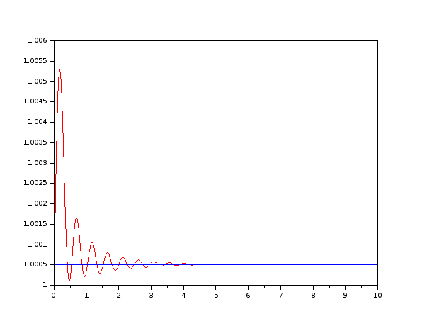
Appendix A Periodicity of when and
When the magnetic field is zero and when , we notice that is periodic, as can be guessed from Figure 2 (which displays for ). Considering a similar graph for , the phenomenon of periodicity has disappeared. The aim of this section is to confirm this numerical observation and to express the period as a function of electrical parameter , explaining where the hypothesis comes into play.
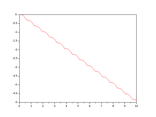
Proposition A.1.
Let . Then is periodic with period .
Proof.
We recall the matrix associated with the Kramers-Fokker-Planck operator when :
The eigenvalues of are and , each with multiplicity , explicitly given by
The matrix is diagonalizable, and we let denote the change-of-basis matrix from the canonical basis to the basis of eigenvectors,
The matrix can be written as
| (60) |
To show that is periodic, we must show that there exists such that
because , according to Proposition 3.1, we have that
therefore, the question amounts to showing the periodicity of the matrix in the sense introduced above. That is to say we are looking for a real such that
and using the fact that
we observe that
In particular, we take , we get , this shows the periodicity of when with period . ∎
Appendix B Numerical illustrations of main results
B.1. Spectral abscissa of .
In the table below we calculate numerically, using Scilab, the values of the spectral abscissa of the matrix which exactly equals in comparing those with the values of by setting and taking several values of .
| b | Spectral abscissa | |
|---|---|---|
| 5 | 0.221337 | 0.56 |
| 10 | 0.0992201 | 0.14 |
| 100 | 0.0013940 | 0.0014 |
| 200 | 0.0003496 | 0.00035 |
| 800 | 0.0000219 | 0.0000219 |
We observe in the previous table that when increases, the spectral gap of the operator , which coincides with the spectral abscissa of the matrix , approaches . In particular this confirms the asymptotics when of . Physically, this represents the rate of return to the equilibrium, and our result therefore serves to quantify the influence of a large magnetic field slowing down the rate of return to the equilibrium.
B.2. Regime when .
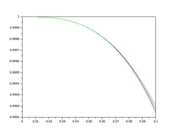
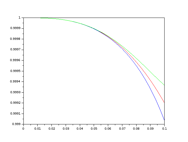
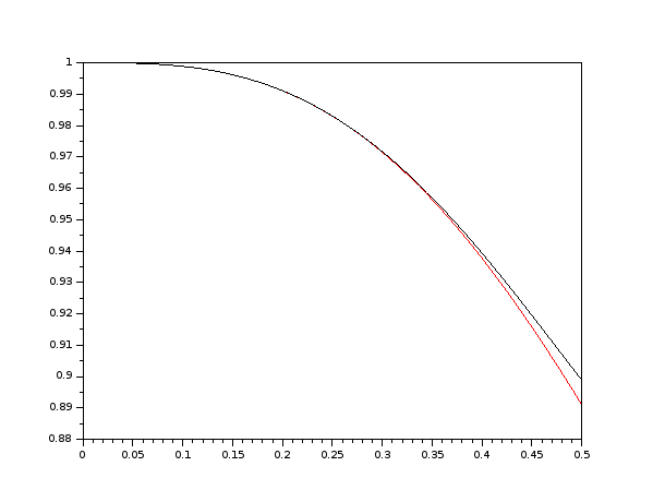
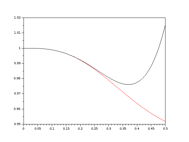
In this part, we will give some numerical illustrations in small time of the norm of . This is the rate of return to the equilibrium for in a regime where is significantly greater than . By observing Figures 4 and 4, where we draw the exact exponential norm and its associated approximations given in Proposition 1.4 with a polynomial error of order . We note that when we increase the magnetic field, the error increases, which is to be expected because our approximations are taken in the regime where is sufficiently small. Then, in Figures 6 and 6, we draw the exact norm with the polynomial given in Proposition 1.4 of order . We observe that when we increase the magnetic field the error increases (see Figure 6).
B.3. Regime when .
In this part, we will give numerical illustrations which illustrate the uniform estimates obtained in Proposition 1.5. Above all, we compare the deviations
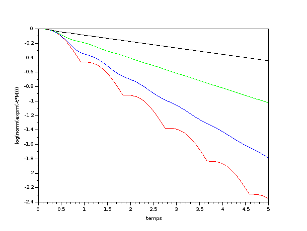
with the approximations given in Proposition 1.5. We observe numerically in Figures 8 and 8 that when we increase the magnetic field the approximation becomes more precise. In examining the figures, it seems that when we increase the magnetic field the norm of the matrix exponential more closely resembles the self-adjoint prediction which equals . In addition, we compare on a logarithmic scale in Figure 10 the exponential norm when and . We observe that the non-self-adjoint character seems to disappear when increases.
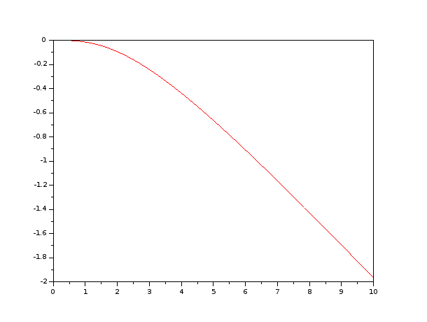
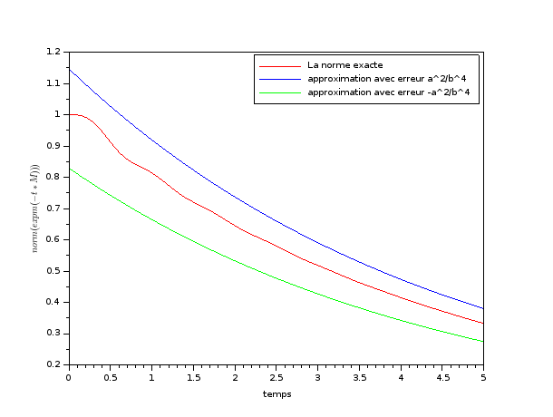
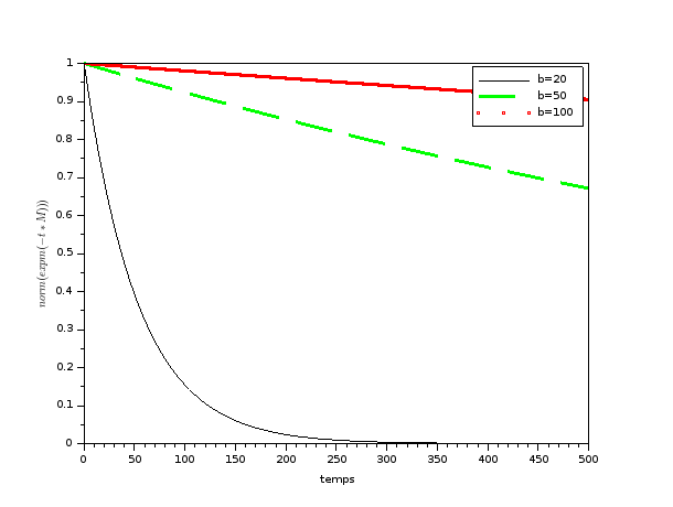
To study the return to the equilibrium, we represent in Figure 10 the norm by taking several values of the magnetic parameter between and . We notice that when the return to equilibrium appears at a time between and , while when on a time scale is equal to , showing that the return to the equilibrium is weaker. Consequently, we see that the magnetic field slows the return to equilibrium.

B.4. Long time regime
In this part we will give numerical illustrations which illustrate the result obtained in Proposition 1.6. As mentioned in the introduction, the result of Proposition 1.6 shows that there is such that if we assume that
then
One can show that the norm of the spectral projector associated with is
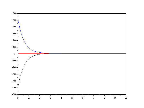
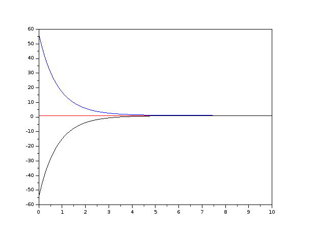
In Figure 12, we draw the behavior in time of the function and the norm exactof the spectral projector when the electric parameter is and the magnetic parameter is . We can observe that over time the function gets closer to the exact norm of . Then, in Figures 12 and 13, we compare the function and the approximations and when and or respectively with the constant . Note that in the two figures the curve of the function lies well between the two curves associated with the approximations cited just before. In addition, from a certain time between and for Figure 12 (when ), we see that the error between the three curves becomes very small. Whereas in Figure 13 and when , a similar decrease of the error appears when the time is between and instead. In conclusion, the estimate given in Proposition 1.6 becomes more precise when the magnetic field is increased.
Acknowledgments
The author is grateful to Joe Viola for his important continued help and advice throughout the creation of this work. The author thanks also the Centre Henri Lebesgue ANR-11-LABX-0020-01 for his support.
References
- [AV14] Alexandru Aleman and Joe Viola. Singular-value decomposition of solution operators to model evolution equations. International Mathematics Research Notices, 2015(17):8275–8288, 2014.
- [AV18] Alexandru Aleman and Joe Viola. On weak and strong solution operators for evolution equations coming from quadratic operators. Journal of Spectral Theory, 8(1):33–122, 2018.
- [GMM18] M.P. Gualdani, S. Mischler, and C. Mouhot. Factorization of Non-symmetric Operators and Exponential H-theorem. Mémoire (Société mathématique de France). Société Mathématique de France, 2018.
- [HN85] Bernard Helffer and Jean Nourrigat. Hypoellipticité maximale pour des opérateurs polynômes de champs de vecteurs. Progress in Mathematics, 58, 1985.
- [HN04] Frédéric Hérau and Francis Nier. Isotropic hypoellipticity and trend to equilibrium for the fokker-planck equation with a high-degree potential. Archive for Rational Mechanics and Analysis, 171(2):151–218, 2004.
- [HPS09] Michael Hitrik and Karel Pravda-Starov. Spectra and semigroup smoothing for non-elliptic quadratic operators. Mathematische Annalen, 344(4):801–846, 2009.
- [HSV11] Michael Hitrik, Johannes Sjöstrand, and Joe Viola. Resolvent estimates for elliptic quadratic differential operators. arXiv preprint arXiv:1109.4497, 2011.
- [Hym58] John Hymers. A treatise on the theory of algebraical equations. 1858.
- [Kar20] Zeinab Karaki. Trend to the equilibrium for the fokker-planck system with an external magnetic field. Kinetic & Related Models, 13(2):309, 2020.
- [Kar21] Zeinab Karaki. Maximal estimates for the fokker–planck operator with magnetic field. Journal of Spectral Theory, 11(3):1179–1213, 2021.
- [NH05] Francis Nier and Bernard Helffer. Hypoelliptic estimates and spectral theory for Fokker-Planck operators and Witten Laplacians. Springer, 2005.
- [Ris98] H Risken. The fokker-plank equation, 3rd printing, 1998.
- [Sai19] Mona Ben Said. Global subelliptic estimates for kramers–fokker–planck operators with some class of polynomials. Journal of the Institute of Mathematics of Jussieu, pages 1–37, 2019.
- [Ser] Denis Serre. Matrices:Theory and Applications.
- [Sjö74] Johannes Sjöstrand. Parametrices for pseudodifferential operators with multiple characteristics. Arkiv för Matematik, 12(1):85–130, 1974.
- [SNV20] Mona Ben Said, Francis Nier, and Joe Viola. Quaternionic structure and analysis of some kramers–fokker–planck operators. Asymptotic Analysis, 119(1-2):87–116, 2020.
- [Vil09] Cédric Villani. Hypocoercivity. Number 949-951. American Mathematical Soc., 2009.
- [Vio13] Joe Viola. Spectral projections and resolvent bounds for partially elliptic quadratic differential operators. Journal of Pseudo-Differential Operators and Applications, 4(2):145–221, 2013.