Joint Learning of Salient Object Detection,
Depth Estimation and Contour Extraction

Abstract

Benefiting from color independence, illumination invariance and location discrimination attributed by the depth map, it can provide important supplemental information for extracting salient objects in complex environments. However, high-quality depth sensors are expensive and can not be widely applied. While general depth sensors produce the noisy and sparse depth information, which brings the depth-based networks with irreversible interference. In this paper, we propose a novel multi-task and multi-modal filtered transformer (MMFT) network for RGB-D salient object detection (SOD). Specifically, we unify three complementary tasks: depth estimation, salient object detection and contour estimation. The multi-task mechanism promotes the model to learn the task-aware features from the auxiliary tasks. In this way, the depth information can be completed and purified. Moreover, we introduce a multi-modal filtered transformer (MFT) module, which equips with three modality-specific filters to generate the transformer-enhanced feature for each modality. The proposed model works in a depth-free style during the testing phase. Experiments show that it not only significantly surpasses the depth-based RGB-D SOD methods on multiple datasets, but also precisely predicts a high-quality depth map and salient contour at the same time. And, the resulted depth map can help existing RGB-D SOD methods obtain significant performance gain. The source code will be publicly available at https://github.com/Xiaoqi-Zhao-DLUT/MMFT.

I Introduction

Salient object detection (SOD) imitates the human visual attention mechanism to search attentive areas or objects from a scene and precisely segment them. As a basic computer vision task, SOD has been applied in many other tasks such as object tracking [2], image caption [3], video object segmentation [4] and human matting [5].

In recent years, with the development of depth sensors, the RGB-D SOD task has become a very striking branch in SOD. Depth map has illumination invariance and color independence, which provides RGB image with important geometrical and discriminative information. Most existing RGB-D SOD methods are depth-based, that is, take an RGB image and a depth map as inputs. They usually adopt a two-stream structure [6, 7, 8, 9, 10, 11] and mainly focus on how to effectively conduct the cross-modal fusion. Different from them, the DANet [12] designs a single stream network for efficiency. Either the two-stream methods or the single-stream one all use the depth map as input and deeply involve it into the feature learning process. As we all know, depth maps acquired by active sensors often carry different types of spatial artifacts such as Gaussian noise and hole pixels and show a checkerboard pattern due to the low distance resolution, as shown in Fig. LABEL:fig:STERE_depth_surfacenorm. Thus, the depth-based SOD methods all inevitably face this serious interference problem. Even if a high-quality depth sensor may reduce the noise, as a single-modality device, it still needs to cooperate with other devices to handle complex scenes.

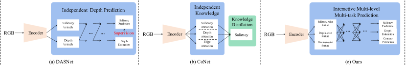
Figure -1: Comparison of three types of depth-free networks.

To this end, we rethink the RGB-D SOD problem. We utilize the multi-task learning (MTL) framework to implement a depth-free model, which can refine the original and coarse depth information to assist salient object detection. In particular, three complementary tasks of depth estimation, saliency and contour prediction are designed and their mutual learning achieves attention focusing and eavesdropping. The MTL network contains three types of modality features (depth-wise, saliency-wise, and contour-wise). How to effectively integrate them will directly affect the final predictions of these three tasks. Motivated by the transformer [13], which can capture global contextual information and establish the long-range dependence, we put forward a multi-modal filtered transformer (MFT) module to drive each modality stream to draw complementary information from other modalities. Specifically, we equip with a multi-modal transformer unit at the highest-level layer. Then, the proposed modality-specific filters (MSFs) are embedded in the transformer unit, which can filter out the task-aware features from the aggregated multi-modal transformer feature. The MTL network equipped with the MFT can predict a high-quality depth map with fine and smooth distribution, as shown in Fig. LABEL:fig:STERE_depth_surfacenorm, which is of greater benefit to saliency detection than the original depth map.

Our main contributions can be summarized as follows:

• We develop a depth-free network based on multi-task learning framework, which can predict the high-quality depth map and saliency map even with low-quality depth supervision. Through full mutual learning among tasks, their predictions all are significantly improved.

• We design a multi-modal filtered transformer module, which embeds the modality-specific filters to achieve the multi-modal feature fusion from the perspective of attention-in-attention. This design can help the task-specific stream to fully acquire useful information from auxiliary task streams.

• Extensive experiments on six benchmark datasets demonstrate that the proposed model performs favorably against the state-of-the-art depth-based and depth-free RGB-D SOD methods under five metrics.

• The predicted depth maps have higher quality than the original ones, which can be applied to previous top-performing depth-based RGB-D SOD methods to improve their performance.

II Related Work

II-A RGB-D Salient Object Detection

According to whether the depth map is required during the testing phase, we classify existing RGB-D SOD methods into two types: depth-based and depth-free one.
Depth-based Methods. In terms of the number of encoding streams, depth-based methods can be further divided into two-stream [14, 15, 16, 9, 17, 6, 8] and single-stream [12] one. PCANet [14] is the first to concentrate on the cross-modal fusion between two streams. Some later works [15, 18, 19, 9] leverage the depth cues to generate spatial attention or channel attention to enhance the RGB features. Sun et al. [20] design a new NAS-based model for the heterogeneous feature fusion in RGB-D SOD and Zhou et al. [11] propose a novel specificity-preserving network to explore the shared information between multi-modal data. These two-stream designs achieve very good performance. Recently, Zhao et al. [12] combine depth map and RGB image from starting to build a single-stream network.
Depth-free Methods. To the best of my knowledge, there are three depth-free models. Inspired by knowledge distillation, A2DELE [21] first transfers the depth knowledge from the depth stream to the RGB stream in the training phase and then only employs the RGB stream for saliency prediction when testing. DASNet [22] utilizes depth information as an error-weighted map to correct the saliency prediction. As shown in Fig. -1 (a), it focuses on the single one task (SOD), the depth branch is just to serve the SOD branch. The most related work is CoNet [23]. As shown in Fig. -1 (b), it first builds three independent branches to generate saliency, depth and edge features under the corresponding supervisions, and then distills all knowledge into the saliency head through multi-modal feature fusion. Different from them, as shown in Fig. -1 (c), we apply multi-task learning and deeply achieve cross-modal interaction to jointly train three task branches until the output. In this way, the depth branch can continuously capture useful multi-scale features from the other two branches to refine the depth information. While CoNet [23] adopts the prediction-to-interaction strategy, which does not implement cross-modal interaction before predicting depth map and salient contour. Thus, its saliency result is very easily corrupted with the noise of the depth modality.

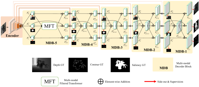
Figure 0: Network pipeline. It consists of a encoder, five multi-modal decoder blocks (MDBs). The multi-modal filtered transformer module is only embedded in the MDB-5. We supervise the side-out of each task branch on multiple levels.

II-B Multi-task Learning

Multi-task learning (MTL) aims to solve multiple tasks by a shared model, which can improve the performance of each individual task via four implicit advantages: the implicit data augmentation, attention focusing, eavesdropping and regularization. In the context of deep Learning, MTL is typically done with two strategies: hard [24] and soft [25] parameter sharing of hidden layers. Hard parameter sharing is the most commonly used approach in neural networks [26, 27, 28], which usually shares the hidden layers among all tasks, while keeping several task-specific output layers. In this paper, we also adopt this strategy. The three tasks share the multi-scale feature extractor, and the task-specific hidden layers in the decoder mutually interweave to achieve attention focusing and regularization under the supervision of ground truth, which guarantees the complementary cues to be fully mined and utilized, thereby making the three tasks complement and reinforce each other.

II-C Transformer in Computer Vision

Transformer was first proposed in  [13]. Due to its outstanding performance, it has revolutionized machine translation and natural language processing. Recently, DETR [29] applies a transformer network for object detection, which greatly simplifies the traditional detection pipeline and shows excellent performance. And then, more and more transformer models are applied to image classification [30], object detection [31], semantic segmentation [32], object tracking [33], video instance segmentation [34], etc. ViT [35] introduces the transformer for image recognition and models an image as a sequence of patches, which attains excellent results compared to the state-of-the-art CNN. The above works show the effectiveness of the transformer in computer vision. However, previous works mainly focus on a single modality. How to utilize the transformer technique to achieve multi-modal fusion is what we are interested in.

III The Proposed Method

III-A Overall Architecture

As shown in Fig.  ‣ II-A, the network consists of five encoder blocks, five multi-modal decoder blocks (MDB) and a multi-modal filtered transformer (MFT) module. The encoder-decoder architecture is based on the FPN [36]. The encoder is built on top of a common backbone network, e.g., VGG [37], ResNet [38] or Res2Net [39], to perform feature extraction of RGB image. Each MDB is used for feature communication among multiple tasks at the corresponding level. There are two reasons to equip with the MFT only on the highest-level features: (1) These features have the lowest spatial resolution, which is helpful to reduce the amount of calculations. (2) As suggested in [40], stand-alone attention layers can better integrate global information that usually exists in the high-level layer.

III-B Multi-modal Decoder Block

To effectively accomplish multi-task learning, it is crucial to cooperatively utilize multi-modal information to enhance each modality branch. As shown in Fig.  ‣ II-A, the basic multi-modal decoder block adopts an information aggregation and distribution structure, dubbed as Squeeze-and-Expand. For each decoder level, we first complete the modality transfer by using the ground truth of depth, saliency and contour to separately supervise their own feature maps. Next, we conduct the multi-modal fusion through the Squeeze operation. In this paper, except for the MDB-5, the other four decoder blocks directly adopt an element-wise addition layer and a convolution layer to achieve feature fusion, as follows:

$$\begin{split}F_{DSC}^{i}=Conv(F_{D}^{i}\oplus F_{S}^{i}\oplus F_{C}^{i}),\quad i\in\left\{1,2,3,4\right\},\end{split}$$ (1)

where $\oplus$ is the element-wise addition and $Conv(\cdot)$ denotes the convolution layer. $F_{DSC}^{i}$ contains the depth-wise, saliency-wise and contour-wise information. And then, we separately combine $F_{DSC}^{i}$ with each modality feature through different convolution layer, coined as the Expand operation. In fact, the Squeeze-and-Expand can be regarded as a multi-modal residual structure. We apply the proposed Squeeze-and-Expand in each MDB to achieve the interaction between different tasks, which can effectively integrate multi-task information and then enhance the characteristics of each task. For this reason, we adopt the form of residual fusion, that is, multi-task aggregation features are used as the residual branch of each task feature to provide complementary information. Because the supervision is enforced in each MDB for each task, the supplementary features of the Squeeze-and-Expand structure are adaptive for different tasks. Finally, the enhanced features ($F_{enD}^{i}$, $F_{enS}^{i}$, $F_{enC}^{i}$) combine the RGB encoder features to participate in the following multi-modal decoder block.

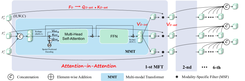
Figure 1: Illustration of the multi-modal filtered transformer module.

III-C Multi-modal Filtered Transformer

In the MDB-5, we design a multi-modal filtered transformer (MFT) module to better perceive the global information. As shown in Fig. 1, it includes the multi-head self-attention, feedforward network and modality-specific filter.
Multi-modal Transformer. Self-Attention (SA) is a fundamental component in standard transformer. Given queries $q$, keys $k$ and values $v$, the attention function is written as:

$$\begin{split}SA(q,k,v)=\mathcal{S}((\frac{{q}{k}^{\top}}{\sqrt{d_{k}}}){v}),\end{split}$$ (2)

where $d_{k}$ is the dimension of $k$ and $\mathcal{S}$ is softmax function. The multi-head self-attention (MHSA) is formulated as:

$${MHSA}(q,k,v)=\mathcal{C}(T_{1},...,T_{nh}){\mathbf{W}^{O}},$$ (3)

$$T_{i}=SA({q}\mathbf{W}_{i}^{q},{k}\mathbf{W}_{i}^{k},{v}\mathbf{W}_{i}^{v}),$$ (4)

where $\mathcal{C}$ is the concatenation operation along channel axis, $\mathbf{W}_{i}^{Q}\in\mathbb{R}^{d_{m}\times d_{k}}$, $\mathbf{W}_{i}^{K}\in\mathbb{R}^{d_{m}\times d_{k}}$, $\mathbf{W}_{i}^{V}\in\mathbb{R}^{d_{m}\times d_{v}}$, and $\mathbf{W}^{O}\in\mathbb{R}^{n_{h}\times d_{v}\times d_{m}}$ are parameter matrices. Please refer to the literature [13] for more details. In this work, we set $nh$ = 8, $d_{m}$ = 384 and $d_{k}$ = $d_{v}$ = $d_{m}$/$nh$ = 12.

Another important unit in transformer is the feedforward network (FFN) module, which is used to enhance the fitting ability of the model. It consists of two linear transformation with a ReLU in between. In the multi-modal transformer, we first aggregate and reshape $F_{D}^{5}$, $F_{S}^{5}$, $F_{C}^{5}$ $\in\mathbb{R}^{C\times H\times W}$ as the transformer input:

$$T_{in}=\mathcal{R}_{1}(\mathcal{C}(F_{D}^{5},F_{S}^{5},F_{C}^{5})),$$ (5)

where $\mathcal{R}_{1}$ reshapes the input feature map to $\mathbb{R}^{C\times N}$. $N={H\times W}$ is the number of features. Next, $T_{in}$ is fed into MHSA and FFN in order, and then the transformer-based multi-modal fusion feature (TMFF) is generated as follows:

$$MHSA_{out}=T_{in}+MHSA(T_{in}+P_{x},T_{in}+P_{x},T_{in}),$$ (6)

$$TMFF=\mathcal{R}_{2}(MHSA_{out}+FFN(MHSA_{out})),$$ (7)

where $\mathcal{R}_{2}$ reshapes the input feature maps to $\mathbb{R}^{C\times H\times W}$ and $P_{x}$ is the spatial positional encoding generated in the same way as DETR [29] to distinguish the position information of the input feature sequence. Since the transformer has many encoder layers, it will dilute the modality-specific information to directly convey TMFF to subsequent layers. To solve this problem, we embed a modality-specific filter to select the useful features.

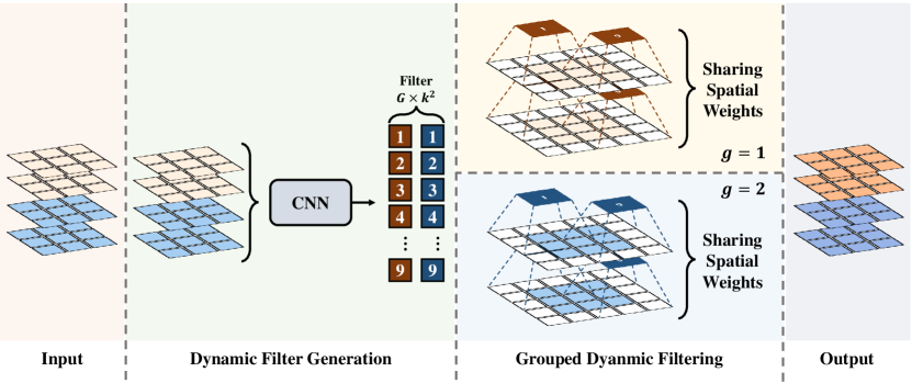
Figure 2: Detailed illustration of the modality-specific filter.

Modality-Specific Filter.Fig. 2 shows the dynamic filter generation and grouped dynamic filtering operation. We follow the spatially-unshared and intragroup-shared principles to design the filter. On the one hand, the differences among the predictions of three tasks are mainly reflected in the location properties of the pixel level. Therefore, we adopt the dynamic kernel to capture the position-specific information, that is, the filter is spatially unshared. On the other hand, the high-level features have rich semantic information in different channels. In order to maintain semantic diversity, we adopt the channel-unshared strategy. However, to save the number of parameters, we refer to the idea of group convolution [41] and adopt a grouping mechanism to achieve the intragroup-shared but intergroup-unshared filtering. The filtering process can be formulated as:

$$Y_{c_{i},h,w}=\sum_{u,v}F_{\lceil\frac{c_{i}}{C_{g}}\rceil,h,w,u+\lfloor\frac{K_{h}}{2}\rfloor,v+\lfloor\frac{K_{w}}{2}\rfloor}X_{c_{i},h+u,w+v},$$ (8)

where $X\in\mathbb{R}^{C_{i}\times H\times W}$ and $Y\in\mathbb{R}^{C_{o}\times H\times W}$ are the input and output features, respectively. $F\in\mathbb{R}^{G\times H\times W\times K_{h}\times K_{w}}$ denotes the dynamic filters, which are yielded by feeding $X$ to two $1$ $\times$ $1$ vanilla convolutional layers. $K_{h}\times K_{w}$ represents the size of the convolution kernel. In this work, we use $3\times 3$ kernel, and set $G=8$ and $C_{g}=C_{i}//G$. For convenience, the offset values relative to the center of the convolution kernel are indexed as $(u,v)\in\Delta_{K}=[-\lfloor\frac{K_{h}}{2}\rfloor,...,\lfloor\frac{K_{h}}{2}\rfloor]\times[-\lfloor\frac{K_{w}}{2}\rfloor,...,\lfloor\frac{K_{w}}{2}\rfloor]\in\mathbb{Z}^{2}$, where $\times$ is the Cartesian product and $\Delta_{K}$ forms a set of two-dimensional coordinate offset.
Attention-in-Attention. In fact, an Attention-in-Attention mechanism is implemented by combining the multi-modal transformer and the modality-specific filter. The self-attention establishes the intrinsic correlation of queries $Q$, keys $K$ and values $V$, which provides a tight information exchange site for an isolated source of the input feature $F$. The frequently cascaded self-attention may gradually weaken the representation capability of features due to the possible accumulation of modality mismatch. For this reason, we build an additional attention barrier outside the internal attention, which takes the output $V_{m-int},m\in\{D,S,C\}$ of the internal attention as the input of the external attention and then utilizes $F_{m}$ to generate attention weight $Q_{m-ext}\cdot K_{m-ext}$. The external attention establishes the secondary relationship among $Q$, $K$ and $V$ through the filtering process. Thus, the internal $V_{m-int}$ is filtered and its enhanced part $V_{m-ext}$ is obtained under the bridging guidance of the external attention. The external-internal attention is actually an attention-in-attention structure. The correspondence between the multi-modal filtered transformer and the Attention-in-Attention is shown in Fig. 1.

III-D Supervision

The total training loss can be written as:

$$\begin{split}L=L_{d}+L_{s}+L_{c}.\end{split}$$ (9)

For the depth estimation, we follow the related works [42, 43, 44] to adopt the combination loss of the L1 and SSIM [45]. For the saliency prediction, we use the weighted IoU loss and binary cross entropy (BCE) loss which have been widely adopted in segmentation tasks. We use the same definitions as in [11, 46, 47, 48]. For the contour prediction, we only adopt the BCE loss.

$$L_{d}= \sum_{n=1}^{N}(l_{ssim}^{(n)}+l_{1}^{(n)})$$ (10)

$$L_{s}= \sum_{n=1}^{N}(l_{bce}^{w(n)}+l_{iou}^{w(n)})$$ (11)

$$L_{c}= \sum_{n=1}^{N}l_{bce}^{(n)}$$ (12)

As described in Sec. III-B, our model is deeply supervised on five groups of outputs, i.e. $N$ = $5$. Besides, for the salient contour estimation, its ground truth ($G_{c}$) is calculated based on the ground-truth saliency map ($G_{s}$). Specifically, we employ the morphological dilation and erosion as follows:

$$\begin{split}G_{c}=D_{m}(G_{s})-E_{m}(G_{s}),\end{split}$$ (13)

where $D(\cdot)$ and $E(\cdot)$ are the dilation and erosion operations, respectively. $m$ denotes a full one filter of size $m\times m$ for erosion and expansion, which is set to $3$ in this paper.

IV Experiments

IV-A Datasets

We evaluate the proposed model on six public RGB-D SOD datasets, which are DUTLF-D [19], STERE [1], NJUD [49], NLPR [50], SIP [51] and LFSD [52]. For comprehensive and fair evaluation, we follow the setting as most previous methods [11, 7, 6, 9, 53, 23, 21]. On the DUTLF-D, we use $800$ samples for training and $400$ samples for testing. For the other five datasets, we use $1,485$ samples from the NJUD and $700$ samples from the NLPR as the training set and the remaining samples in these datasets are used for testing. Besides, we quantitatively compare the predicted depth map of our method and CoNet [23] and other two state-of-the-art depth estimation methods [54, 55] on the SIP. This dataset consists of high-resolution RGB color images and depth maps which are designed to contain multiple salient persons per image. The high-quality camera makes sure that the depth map from the SIP has less noise.

IV-B Evaluation Metrics

For the salient object detection task, we adopt several widely used metrics for quantitative evaluation: F-measure ($F_{\beta}^{max}$) [56], the weighted F-measure ($F_{\beta}^{w}$) [57], mean absolute error ($\mathcal{M}$), the recently released S-measure ($S_{m}$) [58] and E-measure ($E_{m}$) [59]. Besides, we use the Area Under Curve (AUC) as the complementary binary classification evaluation metric. The lower value is better for the $\mathcal{M}$ and the higher is better for others. For the depth estimation task, we use following metrics used by previous works: Root Mean Square Error (RMSE, RMSE (log)), absolute relative error (AbsRel), squared relative error (SqRel) and depth accuracy at various thresholds $1.25$, $1.25^{2}$ and $1.25^{3}$.

IV-C Implementation Details

Our model is implemented based on the Pytorch and trained on one RTX 3090 GPU for $50$ epochs with mini-batch size $12$. The input resolutions of RGB images are resized to $352\times 352$. We adopt some image augmentation techniques to avoid overfitting, including random flipping, rotating, and border clipping. For the optimizer, we use the Adam [60]. For the learning rate, initial learning rate is set to $0.0001$. We adopt the “step” learning rate decay policy, and set the decay size as $30$ and decay rate as $0.9$. Our code will be made publicly available soon.

IV-D Comparisons with State-of-the-art

IV-D1 Quantitative Evaluation

Saliency Evaluation. Since previous RGB-D SOD methods adopt VGG-16, ResNet-50, Res2Net-50 or ResNet-101 as the backbone. For a fair comparison, we separately evaluate the MMFT with different backbones. Tab. I shows performance comparisons in terms of five metrics. We divide these models into depth-based and depth-free. Our method outperforms all of the competitors and obtains the best performance in terms of all metrics on the DUTLF-D, STERE and SIP datasets. It is worth noting that our model achieves significant improvement against the second best depth-free (CoNet [23]) and depth-based (SPNet [11]) models. In addition, the LFSD dataset has only 100 samples, which was originally used for light field saliency research. Most of samples have small variation in depth direction and have large-size foreground, which easily results in that the effect of high-quality depth map is weakened, thereby suppressing the performance of multi-task learning. Tab. II lists the parameters and FLOPs of different methods with superior performance in Tab. I. It can be seen that MMFTs still have advantages against most state-of-the-art models with different backbones under the FLOPs metric. Our method achieves a good balance between accuracy and efficiency while accomplishing multiple tasks.

Besides, we also conduct an extension for RGB SOD task. We use the MMFT, which is trained on RGB-D SOD datasets, to predict depth maps for the images in RGB SOD datasets, and then follow most RGB SOD methods [61, 62, 63, 64, 46, 65, 66, 67, 68] to re-train the MMFT on the DUTS-TR [69] dataset for RGB SOD task. That is, the predicted depth map is used to supervise the depth branch. Tab. III shows the results in terms of five metrics on five RGB SOD datasets. Our method performs favorably against these competitors. Especially, it achieves the best performance on the challenging DUT-OMORN [70] dataset. We note that the proposed method performs slightly bad on the HKU-IS dataset. The reason is possibly as follows: This dataset focuses on multi-object saliency segmentation. Its scenes are usually not complicated and the contrast between the foreground and background is obvious. Thus, the auxiliary effect of depth information for saliency prediction is limited. We think that applying some multi-scale designs such as ASPP or Dense-ASPP can improve the performance on this dataset.
Saliency Contour Evaluation. We evaluate salient contour in terms of two main metrics: $F_{\beta}^{max}$ and $\mathcal{M}$ in Tab. IV. It can be seen that our method surpasses these competitors on all five datasets. Their contours are extracted from the corresponding saliency maps by morphological processing.

TABLE I: Quantitative comparison of different RGB-D SOD methods. $\uparrow$ and $\downarrow$ indicate that the larger scores and the smaller ones are better, respectively. The best three scores are highlighted in red, green and blue. The subscript in each model name is the publication year. The corresponding used backbone network is listed below each model name.

		Depth-based Models																Depth-free Models
Metric		S2MA20	CMWNet20	BBSNet20	BBSNet20	JL-DCF20	UCNet20	PGAR20	HDFNet20	HDFNet20	CDNet21	DFMNet21	DSA2F21	DCF21	HAINet21	RD3D21	SPNet21	A2DELE20	DASNet20	CoNet20	MMFT	MMFT	MMFT	MMFT
		[16]	[9]	[6]	[6]	[53]	[8]	[17]	[7]	[7]	[71]	[72]	[20]	[73]	[74]	[10]	[11]	[21]	[22]	[23]
		VGG-16	VGG-16	VGG-16	ResNet-50	ResNet-101	VGG-16	VGG-16	VGG-16	ResNet-50	VGG-16	ResNet-34	VGG-19	ResNet-50	VGG-16	ResNet-50	Res2Net-50	VGG-16	ResNet-50	ResNet-101	VGG-16	ResNet-50	Res2Net-50	ResNet-101
DUTLF-D	$F_{\beta}^{max}\uparrow$	0.909	0.905	-	-	0.924	-	0.938	0.926	0.930	0.901	-	0.938	0.941	0.932	0.946	-	0.907	-	0.935	0.950	0.955	0.958	0.956
	$F_{\beta}^{w}\uparrow$	0.862	0.831	-	-	0.863	-	0.889	0.865	0.864	0.838	-	0.908	0.909	0.883	0.909	-	0.864	-	0.891	0.909	0.920	0.926	0.924
	$S_{m}\uparrow$	0.903	0.887	-	-	0.905	-	0.920	0.905	0.907	0.886	-	0.921	0.924	0.909	0.931	-	0.886	-	0.919	0.934	0.941	0.942	0.943
	$E_{m}\uparrow$	0.921	0.922	-	-	0.938	-	0.950	0.938	0.938	0.917	-	0.956	0.957	0.939	0.957	-	0.929	-	0.952	0.959	0.967	0.967	0.968
	$\mathcal{M}\downarrow$	0.044	0.056	-	-	0.043	-	0.035	0.040	0.041	0.051	-	0.031	0.030	0.038	0.031	-	0.043	-	0.033	0.029	0.027	0.025	0.024
	$AUC\uparrow$	.9721	.9749	-	-	.9835	-	.9802	.9892	.9884	.9567	-	.9662	.9767	.9777	.9826	-	.9371	-	.9817	.9879	.9893	.9856	.9882
STERE	$F_{\beta}^{max}\uparrow$	0.895	0.911	0.901	0.919	0.913	0.908	0.911	0.918	0.910	0.909	0.914	0.910	0.915	0.919	0.917	0.915	0.892	0.915	0.909	0.931	0.933	0.935	0.931
	$F_{\beta}^{w}\uparrow$	0.825	0.847	0.838	0.858	0.857	0.867	0.856	0.863	0.853	0.855	0.860	0.869	0.873	0.871	0.871	0.873	0.846	0.872	0.866	0.886	0.889	0.894	0.889
	$S_{m}\uparrow$	0.890	0.905	0.896	0.908	0.903	0.903	0.907	0.906	0.900	0.903	0.908	0.897	0.905	0.909	0.911	0.907	0.878	0.910	0.905	0.923	0.926	0.925	0.921
	$E_{m}\uparrow$	0.926	0.930	0.928	0.941	0.937	0.942	0.937	0.937	0.931	0.938	0.939	0.942	0.943	0.938	0.944	0.942	0.928	0.941	0.941	0.949	0.947	0.953	0.952
	$\mathcal{M}\downarrow$	0.051	0.043	0.046	0.041	0.040	0.039	0.041	0.039	0.041	0.041	0.040	0.039	0.037	0.038	0.037	0.037	0.045	0.037	0.037	0.033	0.032	0.031	0.033
	$AUC\uparrow$	.9798	.9846	.9785	.9841	.9846	.9762	.9804	.9870	.9854	.9742	.9849	.9567	.9740	.9849	.9812	.9806	.9355	.9832	.9775	.9873	.9884	.9818	.9820
NLPR	$F_{\beta}^{max}\uparrow$	0.910	0.913	0.921	0.927	0.925	0.916	0.925	0.917	0.927	0.925	0.919	0.916	0.917	0.917	0.927	0.926	0.898	0.929	0.898	0.931	0.935	0.931	0.937
	$F_{\beta}^{w}\uparrow$	0.852	0.856	0.871	0.879	0.882	0.878	0.881	0.869	0.882	0.882	0.877	0.881	0.886	0.881	0.889	0.896	0.857	0.895	0.842	0.885	0.894	0.893	0.900
	$S_{m}\uparrow$	0.915	0.917	0.923	0.930	0.925	0.920	0.930	0.916	0.923	0.930	0.925	0.918	0.921	0.921	0.929	0.927	0.898	0.929	0.908	0.927	0.937	0.933	0.938
	$E_{m}\uparrow$	0.942	0.941	0.948	0.954	0.955	0.955	0.955	0.948	0.957	0.954	0.954	0.952	0.956	0.952	0.959	0.959	0.945	0.961	0.934	0.952	0.958	0.958	0.963
	$\mathcal{M}\downarrow$	0.030	0.029	0.026	0.023	0.022	0.025	0.024	0.027	0.023	0.024	0.024	0.024	0.023	0.025	0.022	0.021	0.029	0.021	0.031	0.024	0.021	0.022	0.020
	$AUC\uparrow$	.9829	.9866	.9838	.9882	. 9889	.9832	.9878	.9861	.9888	.9854	.9894	.9712	.9770	.9842	.9846	.9833	.9447	.9847	.9826	.9878	.9915	.9847	.9867
NJUD	$F_{\beta}^{max}\uparrow$	0.899	0.913	0.926	0.931	0.912	0.908	0.918	0.924	0.922	0.919	0.921	0.917	0.917	0.920	0.923	0.935	0.890	0.911	0.902	0.939	0.938	0.940	0.945
	$F_{\beta}^{w}\uparrow$	0.842	0.857	0.878	0.884	0.869	0.868	0.872	0.881	0.877	0.878	0.879	0.883	0.878	0.879	0.886	0.906	0.843	0.872	0.850	0.900	0.900	0.905	0.909
	$S_{m}\uparrow$	0.894	0.903	0.916	0.921	0.902	0.897	0.909	0.911	0.908	0.913	0.912	0.904	0.903	0.909	0.916	0.924	0.871	0.902	0.895	0.928	0.928	0.927	0.930
	$E_{m}\uparrow$	0.917	0.923	0.937	0.942	0.935	0.934	0.935	0.934	0.932	0.940	0.937	0.937	0.941	0.931	0.942	0.953	0.916	0.936	0.924	0.944	0.944	0.950	0.954
	$\mathcal{M}\downarrow$	0.053	0.046	0.039	0.035	0.041	0.043	0.042	0.037	0.038	0.038	0.039	0.039	0.038	0.038	0.037	0.029	0.047	0.042	0.046	0.033	0.033	0.031	0.030
	$AUC\uparrow$	.9745	.9821	.9828	. 9849	.9812	.9700	.9765	.9843	.9835	.9766	.9845	.9619	.9660	.9810	.9791	.9814	.9296	.9739	.9755	.9879	.9872	.9825	.9832
SIP	$F_{\beta}^{max}\uparrow$	0.891	0.890	0.892	0.902	0.904	0.896	0.893	0.904	0.910	0.888	0.904	0.891	0.900	0.916	0.906	0.916	0.855	0.900	0.883	0.935	0.929	0.931	0.937
	$F_{\beta}^{w}\uparrow$	0.819	0.811	0.820	0.830	0.844	0.836	0.822	0.835	0.848	0.812	0.842	0.829	0.841	0.854	0.845	0.868	0.780	0.836	0.803	0.878	0.875	0.881	0.893
	$S_{m}\uparrow$	0.872	0.867	0.874	0.879	0.880	0.875	0.876	0.878	0.886	0.862	0.885	0.862	0.873	0.886	0.885	0.894	0.828	0.877	0.858	0.909	0.911	0.909	0.917
	$E_{m}\uparrow$	0.913	0.909	0.912	0.917	0.923	0.918	0.912	0.921	0.925	0.905	0.925	0.911	0.921	0.925	0.924	0.931	0.890	0.923	0.909	0.942	0.939	0.943	0.950
	$\mathcal{M}\downarrow$	0.057	0.062	0.056	0.055	0.049	0.051	0.055	0.050	0.047	0.060	0.049	0.057	0.052	0.048	0.048	0.043	0.070	0.051	0.063	0.039	0.038	0.038	0.034
	$AUC\uparrow$	.9585	.9524	.9539	.9555	.9575	.9528	.9610	.9660	.9676	.9361	.9667	.9328	.9391	.9607	.9550	.9609	.8974	.9625	.9485	.9751	.9749	.9682	.9750
LFSD	$F_{\beta}^{max}\uparrow$	0.862	0.900	0.862	0.879	0.887	0.878	0.874	0.860	0.883	0.879	0.888	0.903	0.878	0.877	0.879	0.881	0.858	0.845	0.877	0.892	0.895	0.897	0.884
	$F_{\beta}^{w}\uparrow$	0.772	0.834	0.789	0.814	0.822	0.832	0.800	0.792	0.806	0.821	0.827	0.859	0.824	0.811	0.816	0.823	0.800	0.775	0.815	0.821	0.839	0.843	0.827
	$S_{m}\uparrow$	0.837	0.876	0.845	0.864	0.862	0.864	0.853	0.847	0.854	0.859	0.870	0.883	0.856	0.854	0.858	0.854	0.833	0.827	0.862	0.868	0.881	0.877	0.871
	$E_{m}\uparrow$	0.876	0.908	0.883	0.901	0.902	0.906	0.894	0.883	0.891	0.899	0.906	0.923	0.903	0.892	0.898	0.897	0.875	0.869	0.901	0.900	0.909	0.909	0.897
	$\mathcal{M}\downarrow$	0.094	0.066	0.080	0.072	0.070	0.066	0.074	0.085	0.077	0.073	0.068	0.055	0.071	0.079	0.073	0.071	0.077	0.099	0.071	0.072	0.064	0.063	0.066
	$AUC\uparrow$	.9614	.9734	.9468	.9697	.9668	.9570	.9624	.9640	.9727	.9532	.9741	.9611	.9460	.9662	.9606	.9576	.9087	.9475	.9594	.9746	.9754	.9681	.9625

TABLE II: Efficiency comparisons of the top-performing methods in Tab. I. The best three and worst results are shown in red, green, blue and black, respectively.

Model Nmae	CDNet21	DFMNet21	DSA2F21	DCF21	HAINet21	RD3D21	SPNet21	A2DELE20	DASNet20	CoNet20	MMFT	MMFT	MMFT	MMFT
	[71]	[72]	[20]	[73]	[74]	[10]	[11]	[21]	[22]	[23]
Backbone	VGG-16	ResNet-34	VGG-19	ResNet-50	VGG-16	ResNet-50	Res2Net-50	VGG-16	ResNet-50	ResNet-101	VGG-16	ResNet-50	Res2Net-50	ResNet-101
Parameters (MB)$\downarrow$	32.93	23.44	36.48	47.85	59.82	46.90	150.31	14.90	36.68	43.66	41.38	53.12	75.96	72.13
FLOPs (G)$\downarrow$	72.10	26.32	172.23	17.74	181.41	50.72	67.92	39.07	28.56	27.37	72.82	20.32	25.89	25.50

TABLE III: Quantitative evaluation on RGB SOD datasets. $\uparrow$ and $\downarrow$ indicate that the larger scores and the smaller ones are better, respectively. The best three scores are highlighted in red, green and blue.

Method	Publication	Backbone	DUTS					DUT-OMRON					ECSSD					HKU-IS					PASCAL-S
			$F_{\beta}^{max}\uparrow$	$F_{\beta}^{w}\uparrow$	$S_{m}\uparrow$	$E_{m}\uparrow$	$\mathcal{M}\downarrow$	$F_{\beta}^{max}\uparrow$	$F_{\beta}^{w}\uparrow$	$S_{m}\uparrow$	$E_{m}\uparrow$	$\mathcal{M}\downarrow$	$F_{\beta}^{max}\uparrow$	$F_{\beta}^{w}\uparrow$	$S_{m}\uparrow$	$E_{m}\uparrow$	$\mathcal{M}\downarrow$	$F_{\beta}^{max}\uparrow$	$F_{\beta}^{w}\uparrow$	$S_{m}\uparrow$	$E_{m}\uparrow$	$\mathcal{M}\downarrow$	$F_{\beta}^{max}\uparrow$	$F_{\beta}^{w}\uparrow$	$S_{m}\uparrow$	$E_{m}\uparrow$	$\mathcal{M}\downarrow$
GateNet [68]	ECCV 2020	ResNet-50	0.888	0.809	0.884	0.903	0.040	0.818	0.729	0.837	0.868	0.055	0.945	0.894	0.920	0.943	0.040	0.933	0.881	0.915	0.954	0.033	0.881	0.804	0.854	0.882	0.071
ITSD [67]	CVPR 2020	ResNet-50	0.883	0.824	0.883	0.898	0.041	0.821	0.750	0.839	0.867	0.061	0.947	0.911	0.925	0.932	0.035	0.933	0.893	0.916	0.953	0.031	0.882	0.823	0.859	0.866	0.066
MINet [66]	CVPR 2020	ResNet-50	0.884	0.825	0.883	0.917	0.037	0.810	0.738	0.832	0.873	0.056	0.948	0.911	0.925	0.953	0.034	0.935	0.899	0.919	0.961	0.028	0.880	0.818	0.854	0.897	0.066
GCPA [65]	AAAI 2020	ResNet-50	0.888	0.821	0.889	0.913	0.038	0.812	0.734	0.837	0.869	0.056	0.949	0.903	0.927	0.952	0.035	0.939	0.889	0.920	0.956	0.032	0.882	0.819	0.864	0.899	0.064
F3Net [46]	AAAI 2020	ResNet-50	0.891	0.835	0.887	0.918	0.035	0.813	0.747	0.837	0.876	0.053	0.945	0.912	0.924	0.946	0.033	0.937	0.900	0.916	0.959	0.028	0.882	0.823	0.857	0.892	0.064
VST [64]	ICCV 2021	T2T [75]	0.890	0.828	0.895	0.916	0.037	0.825	0.755	0.849	0.872	0.058	0.951	0.910	0.932	0.957	0.033	0.942	0.898	0.928	0.961	0.029	0.890	0.827	0.871	0.905	0.062
SAMNet [63]	TIP 2021	SAM [63]	0.894	0.840	0.890	0.923	0.035	0.823	0.760	0.844	0.885	0.051	0.952	0.920	0.928	0.958	0.032	0.940	0.905	0.921	0.963	0.027	0.887	0.832	0.862	0.903	0.062
Auto-MSFNet [62]	ACMMM 2021	ResNet-50	0.877	0.841	0.876	0.931	0.034	0.798	0.757	0.831	0.876	0.050	0.941	0.916	0.914	0.954	0.033	0.928	0.904	0.908	0.960	0.027	0.877	0.834	0.851	0.905	0.061
SGL-KRN [61]	AAAI 2021	ResNet-50	0.898	0.847	0.891	0.926	0.034	0.827	0.765	0.845	0.889	0.049	0.946	0.910	0.923	0.942	0.036	0.937	0.902	0.918	0.960	0.029	0.887	0.826	0.856	0.883	0.068
Ours		ResNet-50	0.904	0.844	0.893	0.931	0.034	0.831	0.766	0.849	0.893	0.049	0.960	0.925	0.936	0.958	0.029	0.944	0.901	0.921	0.961	0.029	0.894	0.837	0.871	0.904	0.059

TABLE IV: Quantitative comparison for salient contour extraction.

Method	Backbone	STERE		NJUD		NLPR		SIP		LFSD
		$F_{\beta}^{max}\uparrow$	$\mathcal{M}\downarrow$	$F_{\beta}^{max}\uparrow$	$\mathcal{M}\downarrow$	$F_{\beta}^{max}\uparrow$	$\mathcal{M}\downarrow$	$F_{\beta}^{max}\uparrow$	$\mathcal{M}\downarrow$	$F_{\beta}^{max}\uparrow$	$\mathcal{M}\downarrow$
RD3D [10]	ResNet-50	0.446	0.017	0.480	0.019	0.435	0.014	0.390	0.017	0.440	0.019
SPNet [11]	Res2Net-50	0.393	0.018	0.490	0.018	0.426	0.014	0.384	0.018	0.377	0.022
MMFT	ResNet-50	0.493	0.017	0.501	0.017	0.452	0.013	0.407	0.016	0.473	0.024
MMFT	Res2Net-50	0.480	0.016	0.494	0.017	0.443	0.012	0.394	0.015	0.459	0.017

TABLE V: Quantitative comparison for depth estimation.

Method	Backbone	Error				Accuracy
		RMSE $\downarrow$	RMSE (log) $\downarrow$	Abs Rel $\downarrow$	Sq ReL $\downarrow$	P1 $\uparrow$	P2 $\uparrow$	P3 $\uparrow$
DASNet [22]	ResNet-50	0.378	0.053	0.130	0.078	0.739	0.920	0.984
CoNet [23]	ResNet-101	0.433	0.062	0.149	0.094	0.677	0.907	0.984
TL-Depth [54]	ResNet-101	0.387	0.056	0.134	0.081	0.721	0.911	0.983
LAP-Depth [55]	ResNet-101	0.404	0.049	0.155	0.111	0.771	0.925	0.982
MMFT	ResNet-50	0.353	0.049	0.124	0.070	0.749	0.931	0.986
MMFT	ResNet-101	0.355	0.050	0.124	0.071	0.750	0.927	0.985

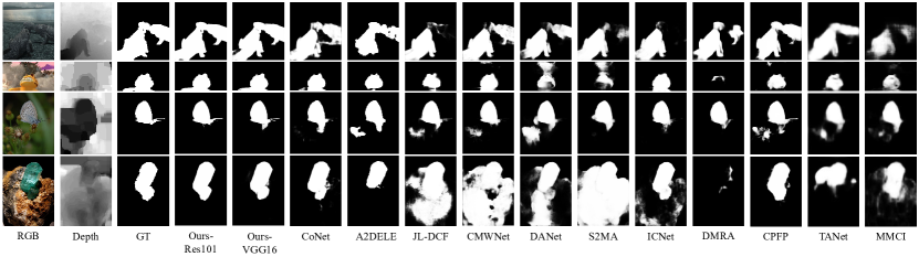
Figure 3: Visual comparison of different RGB-D SOD methods.

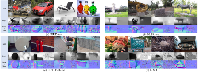
Figure 4: Visual comparison of the predicted depth maps (Left) and the original ones (Right) provided by the RGB-D SOD dataset.

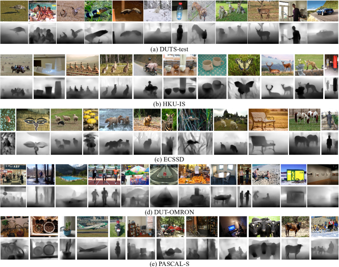
Figure 5: The predicted depth maps on RGB SOD datasets [69, 70, 76, 77, 78].

TABLE VI: Qualitative evaluation of applying the predicted depth map to existing depth-based RGB-D SOD methods. “$\ast$” and “$\ddagger$” mean using the original depth map and ours, respectively.

Method	SIP					STERE					NJUD					NLPR					LFSD
	$F_{\beta}^{max}\uparrow$	$F_{\beta}^{w}\uparrow$	$S_{m}\uparrow$	$E_{m}\uparrow$	$\mathcal{M}\downarrow$	$F_{\beta}^{max}\uparrow$	$F_{\beta}^{w}\uparrow$	$S_{m}\uparrow$	$E_{m}\uparrow$	$\mathcal{M}\downarrow$	$F_{\beta}^{max}\uparrow$	$F_{\beta}^{w}\uparrow$	$S_{m}\uparrow$	$E_{m}\uparrow$	$\mathcal{M}\downarrow$	$F_{\beta}^{max}\uparrow$	$F_{\beta}^{w}\uparrow$	$S_{m}\uparrow$	$E_{m}\uparrow$	$\mathcal{M}\downarrow$	$F_{\beta}^{max}\uparrow$	$F_{\beta}^{w}\uparrow$	$S_{m}\uparrow$	$E_{m}\uparrow$	$\mathcal{M}\downarrow$
Two-stream FPN$\ast$	0.886	0.810	0.847	0.890	0.061	0.882	0.815	0.865	0.899	0.051	0.893	0.834	0.868	0.901	0.052	0.896	0.845	0.889	0.920	0.035	0.844	0.767	0.827	0.864	0.098
Two-stream FPN$\ddagger$	0.903	0.840	0.881	0.919	0.045	0.911	0.850	0.890	0.914	0.042	0.909	0.857	0.894	0.921	0.043	0.914	0.859	0.918	0.945	0.029	0.855	0.787	0.839	0.880	0.088
RD3D$\ast$ [10]	0.906	0.845	0.885	0.924	0.048	0.917	0.871	0.911	0.944	0.037	0.923	0.886	0.916	0.942	0.037	0.927	0.889	0.929	0.959	0.022	0.879	0.816	0.858	0.898	0.073
RD3D$\ddagger$ [10]	0.925	0.879	0.905	0.940	0.038	0.932	0.893	0.922	0.948	0.030	0.937	0.902	0.924	0.947	0.031	0.928	0.893	0.929	0.957	0.022	0.888	0.828	0.867	0.898	0.068
SPNet$\ast$ [11]	0.916	0.868	0.894	0.931	0.043	0.915	0.873	0.907	0.942	0.037	0.935	0.906	0.924	0.953	0.029	0.926	0.896	0.927	0.959	0.021	0.881	0.823	0.854	0.897	0.071
SPNet$\ddagger$ [11]	0.928	0.883	0.907	0.942	0.037	0.931	0.894	0.922	0.952	0.030	0.941	0.910	0.928	0.954	0.029	0.931	0.898	0.930	0.961	0.021	0.882	0.826	0.866	0.901	0.065

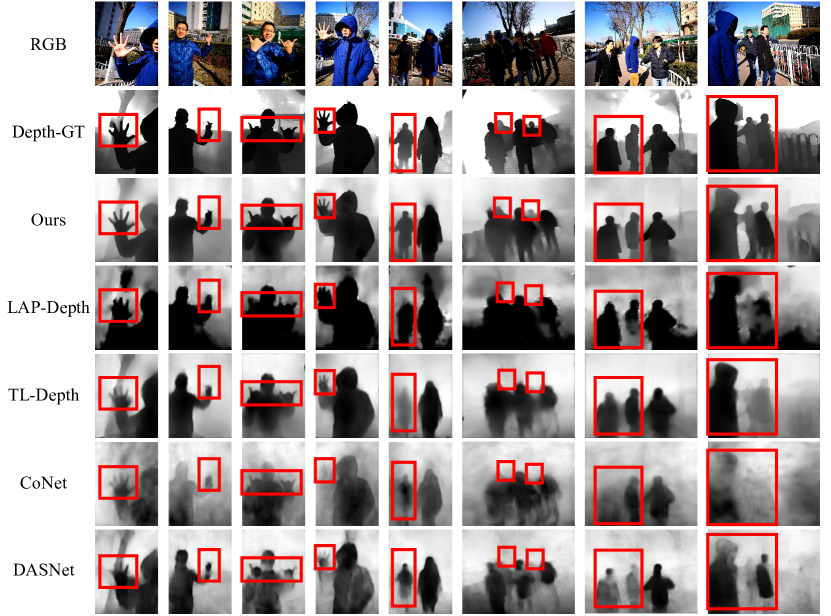
Figure 6: Visual comparisons with several depth estimation methods [54, 55] and CoNet [23] on the SIP dataset [51].

Depth Evaluation. Tab. V shows the results of depth estimation on the SIP dataset in terms of seven common metrics. We compare the proposed method with two depth estimation methods TL-Depth [54] and LAP-Depth [55] and two depth-free RGB-D SOD methods CoNet [23] and DASNet [22]. It can be seen that the proposed method outperforms these models across six metrics. In addition, in order to show the benefits of the predicted depth maps, we apply them to existing depth-based RGB-D SOD methods instead of using the original ones and retrain them, which include the baseline (two-stream FPN) used in [7, 16, 53, 10, 11] and existing top two methods SPNet [11] and RD3D [10]. As shown in Tab. VI, all these models obtain a considerable performance gain.

IV-D2 Qualitative Evaluation

Saliency Evaluation. Fig. 3 illustrates several visual results of different RGB-D SOD approaches. The proposed method yields the results closer to the ground truth in various challenging scenarios. In the $1^{st}$ and $2^{nd}$ rows, we show two examples which have fuzzy depth maps. From the results, it can be observed that our method can segment the objects well while the other methods more or less lose similar areas inside or around salient objects. In the $3^{rd}$ and $4^{th}$ rows, it can be seen that our method has more obvious advantages when handling internal hollow areas, and our saliency maps have sharper contours with the help of the contour decoder.
Depth Evaluation. The proposed method can predict the denoised depth map. As shown in the Fig. LABEL:fig:STERE_depth_surfacenorm and Fig. 4, compared with the original depth map provided by RGB-D SOD dataset, the advantage of our predicted depth map is very significant. To intuitively show the depth map, we utilize it to generate a surface norm map that measures the smoothness of the surface of an object. We can see that the low-quality depth map contains serious Gaussian-like noise and checkerboard pattern. In contrast, the key appearance information such as the contour of the object is better embodied in our depth map. We further qualitative evaluate our depth results on the high-quality SIP [51] dataset, as shown in Fig. 6. It can be seen that our predicted depth maps are closer to the ground-truth and retain the human contours very well (See the $1^{st}$ - $4^{th}$ columns). For complex scenes with multiple objects, our method is still able to perceive the positions of all objects while accurately reflecting the relative depth relationships among them (See the $5^{th}$ - $8^{th}$ columns). Besides, we also show some depth results on several RGB SOD datasets, as shown in Fig. 5. It can be seen that both multiple object and single object cases are accurately measured and even overcome the influence of shadows, which indicates good generalization ability.

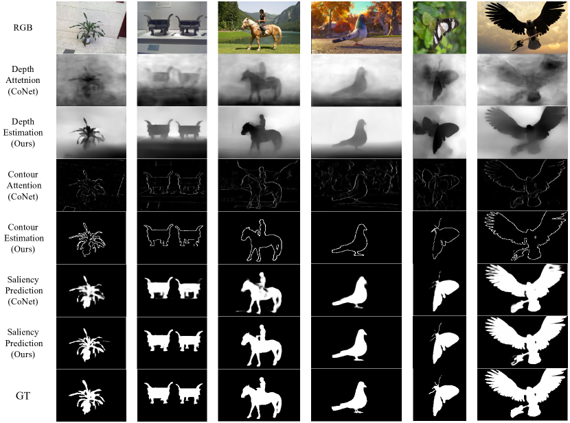
Figure 7: Visual comparisons between ours and CoNet [23] for depth estimation, contour and saliency prediction.

TABLE VII: Ablation experiments of each component for salient object detection. Model 1: the FPN Baseline (Saliency Decoder). Model 2: + Depth Estimation Decoder. Model 3: + Contour Estimation Decoder. Model 4: Without Squeeze-and-Expand in decoder block. Model 5 - Model 9: + Multi-modal Transformer (1, 2, 4, 6 and 8 iterations). Model 10: + Modality-specific Filter. Model 11: Replace the MFT with general Non-local+Convs. Model 12: Replace the MFT with Convs.

Method			SIP					STERE					NJUD					NLPR					LFSD
	Params (MB)$\downarrow$	FLOPs (GB)$\downarrow$	$F_{\beta}^{max}\uparrow$	$F_{\beta}^{w}\uparrow$	$S_{m}\uparrow$	$E_{m}\uparrow$	$\mathcal{M}\downarrow$	$F_{\beta}^{max}\uparrow$	$F_{\beta}^{w}\uparrow$	$S_{m}\uparrow$	$E_{m}\uparrow$	$\mathcal{M}\downarrow$	$F_{\beta}^{max}\uparrow$	$F_{\beta}^{w}\uparrow$	$S_{m}\uparrow$	$E_{m}\uparrow$	$\mathcal{M}\downarrow$	$F_{\beta}^{max}\uparrow$	$F_{\beta}^{w}\uparrow$	$S_{m}\uparrow$	$E_{m}\uparrow$	$\mathcal{M}\downarrow$	$F_{\beta}^{max}\uparrow$	$F_{\beta}^{w}\uparrow$	$S_{m}\uparrow$	$E_{m}\uparrow$	$\mathcal{M}\downarrow$
Model 1	53.54	17.98	0.860	0.766	0.831	0.833	0.062	0.868	0.784	0.849	0.862	0.051	0.872	0.799	0.858	0.847	0.056	0.873	0.810	0.874	0.882	0.038	0.800	0.713	0.777	0.801	0.117
Model 2	55.54	21.35	0.884	0.801	0.857	0.863	0.054	0.890	0.817	0.873	0.881	0.044	0.888	0.834	0.878	0.872	0.047	0.890	0.827	0.885	0.899	0.034	0.827	0.741	0.804	0.829	0.105
Model 3	57.54	24.71	0.896	0.812	0.866	0.874	0.051	0.899	0.830	0.887	0.895	0.042	0.893	0.846	0.888	0.892	0.044	0.896	0.840	0.894	0.910	0.032	0.840	0.762	0.819	0.840	0.099
Model 4	56.62	23.28	0.887	0.787	0.853	0.854	0.056	0.887	0.814	0.877	0.883	0.044	0.884	0.832	0.880	0.878	0.046	0.890	0.823	0.883	0.896	0.035	0.818	0.726	0.796	0.831	0.108
Model 5	60.30	24.89	0.910	0.841	0.882	0.901	0.046	0.911	0.855	0.900	0.916	0.038	0.910	0.869	0.902	0.911	0.038	0.909	0.860	0.911	0.932	0.028	0.851	0.792	0.834	0.855	0.083
Model 6	63.94	25.12	0.913	0.850	0.886	0.909	0.044	0.917	0.866	0.907	0.928	0.037	0.918	0.882	0.908	0.923	0.036	0.912	0.867	0.915	0.940	0.027	0.856	0.799	0.838	0.862	0.080
Model 7	71.22	25.58	0.918	0.857	0.893	0.917	0.043	0.921	0.872	0.908	0.936	0.036	0.924	0.882	0.915	0.930	0.036	0.918	0.873	0.920	0.944	0.026	0.864	0.808	0.846	0.874	0.075
Model 8	78.51	26.05	0.920	0.863	0.897	0.920	0.042	0.924	0.879	0.912	0.943	0.035	0.928	0.886	0.917	0.935	0.034	0.921	0.879	0.922	0.950	0.024	0.872	0.811	0.852	0.883	0.072
Model 9	85.79	26.52	0.917	0.863	0.895	0.919	0.042	0.924	0.878	0.912	0.942	0.035	0.929	0.884	0.913	0.934	0.034	0.921	0.880	0.920	0.949	0.024	0.872	0.808	0.854	0.884	0.072
Model 10	75.96	25.89	0.931	0.881	0.909	0.943	0.038	0.935	0.894	0.925	0.953	0.031	0.940	0.905	0.927	0.950	0.031	0.931	0.893	0.933	0.958	0.022	0.897	0.843	0.877	0.909	0.063
Model 11	76.20	26.12	0.908	0.852	0.883	0.907	0.045	0.921	0.870	0.913	0.932	0.037	0.917	0.877	0.916	0.921	0.037	0.911	0.870	0.913	0.937	0.028	0.855	0.803	0.835	0.857	0.080
Model 12	76.40	27.45	0.894	0.808	0.868	0.879	0.052	0.901	0.834	0.893	0.899	0.042	0.890	0.844	0.889	0.891	0.045	0.898	0.848	0.896	0.914	0.031	0.833	0.754	0.813	0.840	0.102

TABLE VIII: Ablation experiments of each component for depth estimation. Model 1: the FPN Baseline (Depth Estimation Decoder). Model 2: + Saliency Decoder. Model 3: + Contour Estimation Decoder. The others “Model *” correspond to the same model in Tab. VII.

Method	Error				Accuracy
	RMSE $\downarrow$	RMSE (log) $\downarrow$	Abs Rel $\downarrow$	Sq ReL $\downarrow$	P1 $\uparrow$	P2 $\uparrow$	P3 $\uparrow$
Model 1	0.424	0.085	0.180	0.120	0.670	0.851	0.970
Model 2	0.394	0.075	0.166	0.096	0.710	0.882	0.974
Model 3	0.389	0.070	0.161	0.093	0.718	0.890	0.976
Model 4	0.400	0.078	0.171	0.102	0.700	0.871	0.972
Model 5	0.368	0.060	0.147	0.082	0.739	0.904	0.980
Model 6	0.362	0.056	0.143	0.078	0.745	0.912	0.980
Model 7	0.358	0.054	0.140	0.076	0.748	0.917	0.982
Model 8	0.355	0.052	0.137	0.075	0.752	0.922	0.982
Model 9	0.356	0.052	0.138	0.074	0.750	0.921	0.981
Model 10	0.343	0.048	0.120	0.068	0.763	0.931	0.984
Model 11	0.372	0.064	0.150	0.085	0.734	0.900	0.978
Model 12	0.387	0.072	0.170	0.105	0.720	0.874	0.973

TABLE IX: Ablation experiments of each component for contour estimation. Model 1: the FPN Baseline (Contour Estimation Decoder). Model 2: + Saliency Decoder. Model 3: + Depth Estimation Decoder. The others “Model *” correspond to the same model in Tab. VII.

Method	STERE		NJUD		NLPR		SIP		LFSD
	$F_{\beta}^{max}\uparrow$	$\mathcal{M}\downarrow$	$F_{\beta}^{max}\uparrow$	$\mathcal{M}\downarrow$	$F_{\beta}^{max}\uparrow$	$\mathcal{M}\downarrow$	$F_{\beta}^{max}\uparrow$	$\mathcal{M}\downarrow$	$F_{\beta}^{max}\uparrow$	$\mathcal{M}\downarrow$
Model 1	0.414	0.021	0.432	0.019	0.381	0.019	0.332	0.019	0.393	0.026
Model 2	0.436	0.018	0.450	0.021	0.400	0.017	0.348	0.017	0.410	0.023
Model 3	0.442	0.018	0.459	0.020	0.406	0.016	0.356	0.016	0.417	0.022
Model 4	0.430	0.019	0.448	0.022	0.394	0.018	0.340	0.018	0.405	0.023
Model 5	0.454	0.016	0.472	0.018	0.420	0.015	0.366	0.017	0.437	0.020
Model 6	0.460	0.017	0.477	0.019	0.422	0.015	0.372	0.016	0.440	0.019
Model 7	0.465	0.018	0.479	0.019	0.427	0.014	0.380	0.017	0.442	0.019
Model 8	0.468	0.018	0.484	0.019	0.430	0.014	0.385	0.017	0.445	0.019
Model 9	0.466	0.018	0.484	0.019	0.429	0.014	0.386	0.017	0.444	0.019
Model 10	0.480	0.016	0.494	0.017	0.443	0.012	0.394	0.015	0.459	0.017
Model 11	0.459	0.017	0.470	0.019	0.418	0.018	0.364	0.017	0.430	0.020
Model 12	0.440	0.018	0.457	0.020	0.406	0.017	0.350	0.017	0.417	0.022

IV-E Comprehensive Comparison with CoNet

CoNet [23] unidirectionally utilizes depth attention and contour attention to help RGB-D salient object detection, which is not an implementation of multi-task learning. In order to fully demonstrate our superiority and difference, we visualize some results in Fig. 7. Benefiting from the multi-task design and the Squeeze-and-Expand strategy, we obtain better predictions on the three tasks. The smooth body, sharp contour and accurate localization are fully reflected in each task.

IV-F Ablation Studies for Salient Object Detection

In this section, we show the effectiveness of each component for the salient object detection. All the experiments are based on the Res2Net-50 backbone.
Multi-task Learning. We take the FPN with the RGB input and a saliency decoder branch as the baseline. The depth estimation and contour extraction branches are then added to the baseline, respectively. We apply the Squeeze-and-Expand (SE) structure in each decoder branch. As shown in Tab. VII, Model $2$ vs. Model $1$ and Model $3$ vs. Model $2$ show the effectiveness of depth estimation and salient contour extraction for saliency prediction, respectively. It can be seen that the multi-task network (Model $3$) achieves a significant improvement compared to the baseline with the gain of $5.87\%$ and $17.65\%$ in terms of $F_{\beta}^{w}$ and MAE on the challenging STERE dataset. In addition, we remove all SEs to obtain Model $4$, in which three decoder branches are completely independent without any interaction. The performance gap between Model $3$ and Model $4$ indicates the necessity of information interaction among different types of features.
Multi-modal Filtered Transformer. Based on Model $3$, we verify the benefits of multi-modal transformer (MMT) and modality-specific filter (MSF) in multi-modal filtered transformer (MFT), as shown in Tab. VII. Model $5$ performs much better than Model $3$, which shows the superiority of multi-modal transformer in the SOD. We conduct a series of experiments about the number of iterations in MMT. The Model $8$ with six MMT iterations achieves the best accuracy among Model $5$ - Model $9$. Then, we equip with the MSF and find that Model $10$ achieves further performance improvement over Model $8$, which verifies the effectiveness of the MSF. In addition, we replace the MFT module with some convolution layers or general non-local module, and a similar number of parameters and computation are preserved. Compared to Model $11$ and Model $12$, Model $10$ has obvious performance advantage.

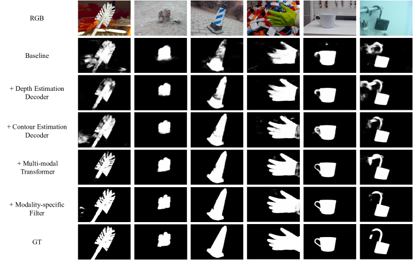
Figure 8: Visual results of each component.

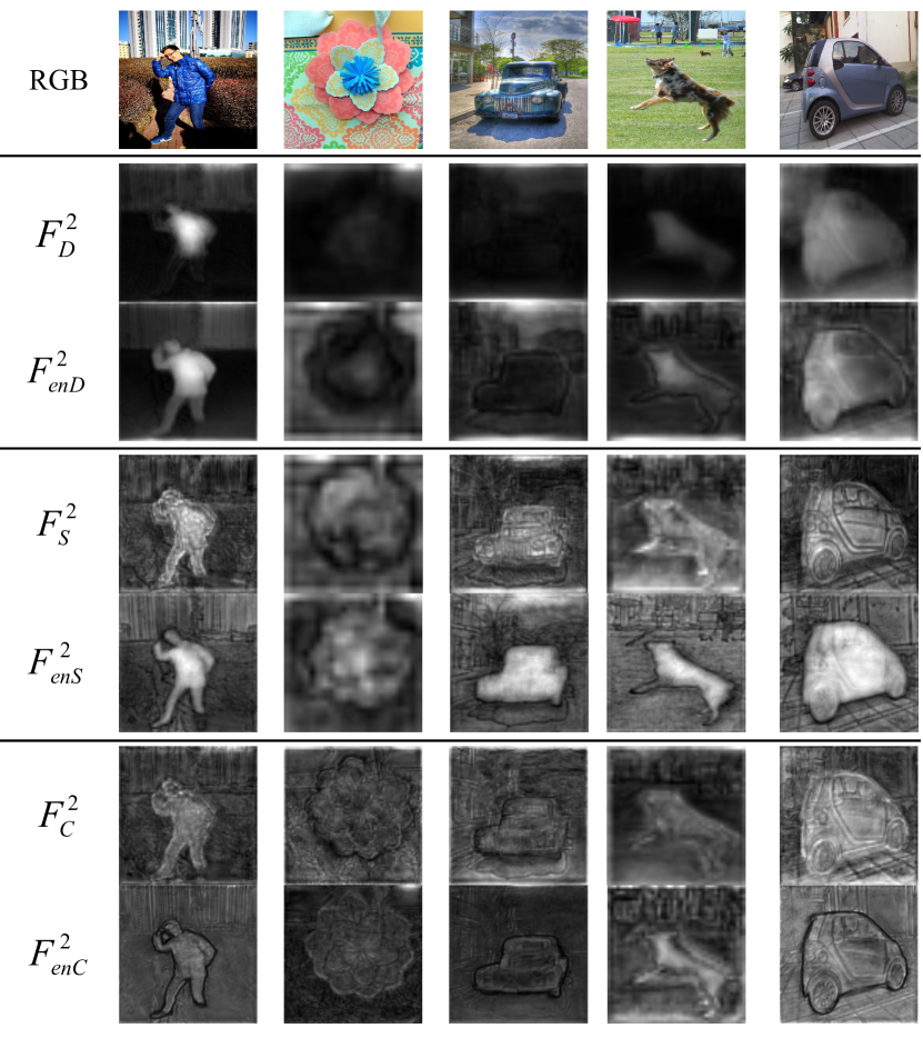
Figure 9: Visualization of each modality feature in MDB-2.

Visual Analyses. Fig. 8 shows visual results of the ablation study. Firstly, we can see that “+ Depth Estimation Decoder” model localizes salient object more precisely compared to “Baseline” model. Next, “+ Contour Estimation Decoder” model further refine the saliency prediction along the contour. Thirdly, “+ Multi-modal Transformer” model integrates the advantages of three kinds of modalities. Finally, “+ Modality-specific Filter” model significantly refines the details of salient objects. To intuitively show the effectiveness of the proposed Squeeze-and-Expand (SE) structure, we take MDB-2 as an example to visualize each modality feature before and after SE operation in Fig. 9. It can be seen that $F_{enD}^{2}$, $F_{enS}^{2}$ and $F_{enC}^{2}$ all have more precise positions and contours compared with $F_{D}^{2}$, $F_{S}^{2}$ and $F_{c}^{2}$. This verifies that SE can effectively supplement complementary information among different modalities.

IV-G Ablation studies for Depth and Salient Contour Estimation

We evaluate each component for depth estimation and contour prediction. All the experiments are based on the Res2Net-50 backbone. As shown in Tab. VIII and Tab. IX, Model $2$ vs. Model $1$ and Model $3$ vs. Model $2$ show the benefits of the multi-task learning. The performance gap between Model $3$ and Model $4$ indicates the necessity of embedding Squeeze-and-Expand structure in the decoder to interact information among different types of features. Model $10$ vs. Model $3$ verifies the benefit of the multi-modal filtered transformer. Model $10$ has obvious performance advantage over Model $11$ and Model $12$ under a similar number of parameters and comparable computational cost.

V More Insightful Analyses

V-A Why can different tasks promote each other?

In this work, the three tasks all require to capture vital position and appearance cues about the objects, and they are complementary. Specifically, depth map contains natural contrast information, which provides useful guidance for saliency and contour positioning. Object contour is one of important attributes of saliency and depth modalities. Accurate contour prediction will improve the quality of depth and saliency estimation. Saliency map provides a fine foreground segmentation and its internal consistency is helpful to avoid the checkerboard pattern in depth estimation.

In a multi-task learning network, the backpropagation acts on multiple task branches in parallel. Different branches share hidden layer features of multiple scales from the encoder network, and the feature representations used for specific task in these hidden layers are also used by the other tasks. These prompt multiple tasks to be learned together. Based on the multi-task framework, the implicit data augmentation, attention focusing, eavesdropping and regularization guarantee the above-mentioned complementary cues to be fully mined and utilized, thereby making the three pixel-level dense prediction tasks promote each other.

V-B Why high-quality depth can be estimated?

It is an interesting phenomenon that we obtain high-quality depth predictions under the supervision of poor depth maps. The regularization of multi-task learning can balance the performance of different tasks since each task is actually also regularized by the other tasks. If the predicted depth map approaches the poor ground-truth, it will interfere with the predictions of the other two tasks. To resist the negative effect, the multi-task network interactively adjusts and balances each task prediction. Thus, the depth branch absorbs useful information from saliency and contour branches, e.g., the clues about smooth object region and sharp object contour.

Moreover, due to the uncertainty of noise, the poor depth ground-truth is more difficulty fitted than good depth map. As reflected in [79], when using the gradient descent to optimize convolutional neural network, it is not sensitive to noise and will be faster and easier to learn to get a more natural-looking image. In other words, CNN offers high impedance to noise. Therefore, our model can easily learn important and effective signals in the depth map during the training process.

In summary, multi-task learning strategy enables the model to balance the losses and gradients of different tasks. By suppressing noise and mining complementary information from the auxiliary tasks, a good depth map is obtained.

VI Positive Impacts

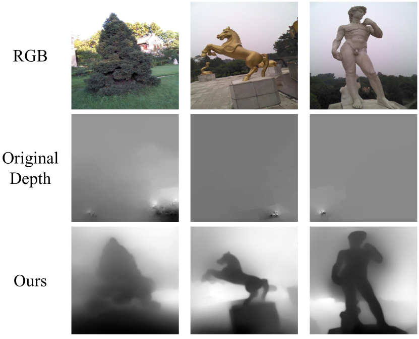
Figure 10: The case of depth sensor malfunction.

For the salient object detection task, this work has many positive impacts on the community and practical applications.
First, the resulted depth map from our network can help existing depth-based RGB-D SOD methods obtain significant performance gain, as shown in Tab. VI.
Second, once the depth-based method cascades our network and adopt the depth map predicted from our network as the input can help the depth-based network get rid of the dependence on the depth-sensor to have a more flexible applicability.
Third, as shown in Fig. 10, these examples are from the NLPR [50] dataset. We can see that the original depth can not capture any depth information, which illustrates the depth sensor do suffer from stability problems, but our approach can avoid such failure predictions.
Last but not the least, we know that one of the important applications of saliency detection is background bokeh. In real smartphones such as the Huawei P40 pro, achieving background bokeh in portrait mode relies on the ToF camera to provide depth information to project bokeh and focus. Different from them, our method not only saves the cost of the ToF camera, but also can provide two modes of AI-assisted background bokeh. They are the extreme mode and the progressive mode with the guidance of saliency map and depth map, respectively.

VII Limitation and Rethinking

In this work, we design three tasks and interact three modal information closely based on our squeeze-and-expand structure. Although we can see a significant improvement in the overall performance under quantitative metrics, there are still some limitations. As shown in Fig. 11, when one task fails, it possibly affects the predictions of the other two tasks. In order to avoid this problem, we give three possible solutions: (1) Construct a dynamic balancing unit to balance the contribution of the features of each modality to the features of other modalities, which can alleviate the negative impact. (2) Set up a task feedback mechanism that scores the confidence of the prediction results through a regression network. According to the scores, the intermediate features generated by each task branch are weighted to refine the prediction results using a recurrent style. (3) Design a balanced loss function to build a controllable sparsity among three tasks. These will be studied in the future.

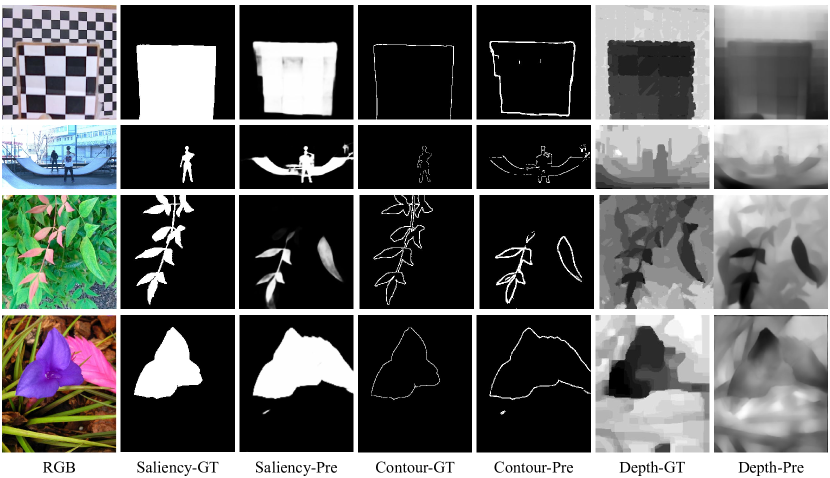
Figure 11: Failure cases.

VIII Conclusion

In this work, we propose a multi-task and multi-modal filtered transformer (MMFT) network for depth-free RGB-D salient object detection. First, we design three related dense prediction tasks: depth estimation, salient object detection and contour prediction. The three modal features rely on the Squeeze-and-Expand structure to deeply achieve task-aware information exchanges. Next, to fully integrate the three kinds of features in high level from the global perspective, we use the transformer technique to achieve multi-modal feature fusion and embed the modality-specific filter to better enhance each modality feature. Through multi-task learning, the depth decoder branch can capture appearance and boundary cues from the other two branches to complete and purify the depth information, thereby predicting a high-quality depth map. Extensive experiments show that our model performs well on the six RGB-D SOD datasets. By using the predicted depth map, the performance of previous state-of-the-art methods can be consistently improved.

References

- [1] Y. Niu, Y. Geng, X. Li, and F. Liu, “Leveraging stereopsis for saliency analysis,” in CVPR, 2012, pp. 454–461.
- [2] V. Mahadevan and N. Vasconcelos, “Saliency-based discriminant tracking,” in CVPR, 2009.
- [3] H. Fang, S. Gupta, F. Iandola, R. K. Srivastava, L. Deng, P. Dollár, J. Gao, X. He, M. Mitchell, J. C. Platt et al., “From captions to visual concepts and back,” in CVPR, 2015, pp. 1473–1482.
- [4] X. Zhao, Y. Pang, J. Yang, L. Zhang, and H. Lu, “Multi-source fusion and automatic predictor selection for zero-shot video object segmentation,” in ACM MM, 2021, pp. 2645–2653.
- [5] R. Deora, R. Sharma, and D. S. S. Raj, “Salient image matting,” arXiv preprint arXiv:2103.12337, 2021.
- [6] D.-P. Fan, Y. Zhai, A. Borji, J. Yang, and L. Shao, “Bbs-net: Rgb-d salient object detection with a bifurcated backbone strategy network,” in ECCV, 2020, pp. 275–292.
- [7] Y. Pang, L. Zhang, X. Zhao, and H. Lu, “Hierarchical dynamic filtering network for rgb-d salient object detection,” in ECCV, 2020, pp. 235–252.
- [8] J. Zhang, D.-P. Fan, Y. Dai, S. Anwar, F. S. Saleh, T. Zhang, and N. Barnes, “Uc-net: Uncertainty inspired rgb-d saliency detection via conditional variational autoencoders,” in CVPR, 2020, pp. 8582–8591.
- [9] G. Li, Z. Liu, L. Ye, Y. Wang, and H. Ling, “Cross-modal weighting network for rgb-d salient object detection,” in ECCV, 2020, pp. 665–681.
- [10] Q. Chen, Z. Liu, Y. Zhang, K. Fu, Q. Zhao, and H. Du, “Rgb-d salient object detection via 3d convolutional neural networks,” in AAAI, vol. 35, no. 2, 2021, pp. 1063–1071.
- [11] T. Zhou, H. Fu, G. Chen, Y. Zhou, D.-P. Fan, and L. Shao, “Specificity-preserving rgb-d saliency detection,” in CVPR, 2021, pp. 4681–4691.
- [12] X. Zhao, L. Zhang, Y. Pang, H. Lu, and L. Zhang, “A single stream network for robust and real-time rgb-d salient object detection,” in ECCV, 2020, pp. 646–662.
- [13] A. Vaswani, N. Shazeer, N. Parmar, J. Uszkoreit, L. Jones, A. N. Gomez, L. Kaiser, and I. Polosukhin, “Attention is all you need,” in NeurIPS, 2017, p. 5998–6008.
- [14] H. Chen and Y. Li, “Progressively complementarity-aware fusion network for rgb-d salient object detection,” in CVPR, 2018, pp. 3051–3060.
- [15] J.-X. Zhao, Y. Cao, D.-P. Fan, M.-M. Cheng, X.-Y. Li, and L. Zhang, “Contrast prior and fluid pyramid integration for rgbd salient object detection,” in CVPR, 2019.
- [16] N. Liu, N. Zhang, and J. Han, “Learning selective self-mutual attention for rgb-d saliency detection,” in CVPR, 2020, pp. 13 756–13 765.
- [17] S. Chen and Y. Fu, “Progressively guided alternate refinement network for rgb-d salient object detection,” in ECCV, 2020, pp. 520–538.
- [18] G. Li, Z. Liu, and H. Ling, “Icnet: Information conversion network for rgb-d based salient object detection,” IEEE TIP, vol. 29, pp. 4873–4884, 2020.
- [19] Y. Piao, W. Ji, J. Li, M. Zhang, and H. Lu, “Depth-induced multi-scale recurrent attention network for saliency detection,” in ICCV, 2019, pp. 7254–7263.
- [20] P. Sun, W. Zhang, H. Wang, S. Li, and X. Li, “Deep rgb-d saliency detection with depth-sensitive attention and automatic multi-modal fusion,” in CVPR, 2021, pp. 1407–1417.
- [21] Y. Piao, Z. Rong, M. Zhang, W. Ren, and H. Lu, “A2dele: Adaptive and attentive depth distiller for efficient rgb-d salient object detection,” in CVPR, 2020, pp. 9060–9069.
- [22] J. Zhao, Y. Zhao, J. Li, and X. Chen, “Is depth really necessary for salient object detection?” in ACM MM, 2020, pp. 1745–1754.
- [23] W. Ji, J. Li, M. Zhang, Y. Piao, and H. Lu, “Accurate rgb-d salient object detection via collaborative learning,” in ECCV, 2020, pp. 52–69.
- [24] R. Caruana, “Multitask learning: A knowledge-based source of inductive bias,” in ICML, 1993, pp. 41–48.
- [25] L. Duong, T. Cohn, S. Bird, and P. Cook, “Low resource dependency parsing: Cross-lingual parameter sharing in a neural network parser,” in ACL, 2015, pp. 845–850.
- [26] M. Long, Z. CAO, J. Wang, and P. S. Yu, “Learning multiple tasks with multilinear relationship networks,” in NeurIPS, 2017, pp. 1593–1602.
- [27] O. Sener and V. Koltun, “Multi-task learning as multi-objective optimization,” in NeurIPS, 2018, pp. 525–536.
- [28] S. Ruder, J. Bingel, I. Augenstein, and A. Søgaard, “Latent multi-task architecture learning,” in AAAI, vol. 33, no. 01, 2019, pp. 4822–4829.
- [29] N. Carion, F. Massa, G. Synnaeve, N. Usunier, A. Kirillov, and S. Zagoruyko, “End-to-end object detection with transformers,” in ECCV, 2020, pp. 213–229.
- [30] M. Chen, A. Radford, R. Child, J. Wu, H. Jun, D. Luan, and I. Sutskever, “Generative pretraining from pixels,” in ICLR, 2020, pp. 1691–1703.
- [31] K. Chen, J. K. Chen, J. Chuang, M. Vázquez, and S. Savarese, “Topological planning with transformers for vision-and-language navigation,” arXiv preprint arXiv:2012.05292, 2020.
- [32] S. Zheng, J. Lu, H. Zhao, X. Zhu, Z. Luo, Y. Wang, Y. Fu, J. Feng, T. Xiang, P. H. Torr et al., “Rethinking semantic segmentation from a sequence-to-sequence perspective with transformers,” arXiv preprint arXiv:2012.15840, 2020.
- [33] X. Chen, B. Yan, J. Zhu, D. Wang, X. Yang, and H. Lu, “Transformer tracking,” arXiv preprint arXiv:2103.15436, 2021.
- [34] Y. Wang, Z. Xu, X. Wang, C. Shen, B. Cheng, H. Shen, and H. Xia, “End-to-end video instance segmentation with transformers,” arXiv preprint arXiv:2011.14503, 2020.
- [35] A. Dosovitskiy, L. Beyer, A. Kolesnikov, D. Weissenborn, X. Zhai, T. Unterthiner, M. Dehghani, M. Minderer, G. Heigold, S. Gelly et al., “An image is worth 16x16 words: Transformers for image recognition at scale,” arXiv preprint arXiv:2010.11929, 2020.
- [36] T.-Y. Lin, P. Dollár, R. Girshick, K. He, B. Hariharan, and S. Belongie, “Feature pyramid networks for object detection,” in CVPR, 2017, pp. 2117–2125.
- [37] K. Simonyan and A. Zisserman, “Very deep convolutional networks for large-scale image recognition,” arXiv preprint arXiv:1409.1556, 2014.
- [38] K. He, X. Zhang, S. Ren, and J. Sun, “Deep residual learning for image recognition,” in CVPR, 2016, pp. 770–778.
- [39] S. Gao, M.-M. Cheng, K. Zhao, X.-Y. Zhang, M.-H. Yang, and P. H. Torr, “Res2net: A new multi-scale backbone architecture,” IEEE TPAMI, 2019.
- [40] N. Parmar, P. Ramachandran, A. Vaswani, I. Bello, A. Levskaya, and J. Shlens, “Stand-alone self-attention in vision models,” in NeurIPS, 2019, pp. 68–80.
- [41] S. Xie, R. Girshick, P. Dollár, Z. Tu, and K. He, “Aggregated residual transformations for deep neural networks,” in CVPR, 2017, pp. 1492–1500.
- [42] S. Pillai, R. Ambruş, and A. Gaidon, “Superdepth: Self-supervised, super-resolved monocular depth estimation,” in ICRA, 2019, pp. 9250–9256.
- [43] R. Ranftl, K. Lasinger, D. Hafner, K. Schindler, and V. Koltun, “Towards robust monocular depth estimation: Mixing datasets for zero-shot cross-dataset transfer,” IEEE TPAMI, 2020.
- [44] M. Ocal and A. Mustafa, “Realmonodepth: Self-supervised monocular depth estimation for general scenes,” arXiv preprint arXiv:2004.06267, 2020.
- [45] Z. Wang, E. P. Simoncelli, and A. C. Bovik, “Multiscale structural similarity for image quality assessment,” in The Thrity-Seventh Asilomar Conference on Signals, Systems & Computers, 2003, vol. 2, 2003, pp. 1398–1402.
- [46] J. Wei, S. Wang, and Q. Huang, “F3net: Fusion, feedback and focus for salient object detection,” in AAAI, 2020, pp. 12 321–12 328.
- [47] D.-P. Fan, G.-P. Ji, T. Zhou, G. Chen, H. Fu, J. Shen, and L. Shao, “Pranet: Parallel reverse attention network for polyp segmentation,” in MICCAI. Springer, 2020, pp. 263–273.
- [48] X. Zhao, L. Zhang, and H. Lu, “Automatic polyp segmentation via multi-scale subtraction network,” in MICCAI. Springer, 2021.
- [49] R. Ju, L. Ge, W. Geng, T. Ren, and G. Wu, “Depth saliency based on anisotropic center-surround difference,” in ICIP, 2014, pp. 1115–1119.
- [50] H. Peng, B. Li, W. Xiong, W. Hu, and R. Ji, “Rgbd salient object detection: A benchmark and algorithms,” in ECCV, 2014, pp. 92–109.
- [51] D.-P. Fan, Z. Lin, Z. Zhang, M. Zhu, and M.-M. Cheng, “Rethinking rgb-d salient object detection: Models, data sets, and large-scale benchmarks,” IEEE TNNLS, vol. 32, no. 5, pp. 2075–2089, 2020.
- [52] N. Li, J. Ye, Y. Ji, H. Ling, and J. Yu, “Saliency detection on light field,” in CVPR, 2014, pp. 2806–2813.
- [53] K. Fu, D.-P. Fan, G.-P. Ji, and Q. Zhao, “Jl-dcf: Joint learning and densely-cooperative fusion framework for rgb-d salient object detection,” in CVPR, 2020, pp. 3052–3062.
- [54] I. Alhashim and P. Wonka, “High quality monocular depth estimation via transfer learning,” arXiv preprint arXiv:1812.11941, 2018.
- [55] M. Song, S. Lim, and W. Kim, “Monocular depth estimation using laplacian pyramid-based depth residuals,” IEEE TCSVT, 2021.
- [56] R. Achanta, S. Hemami, F. Estrada, and S. Süsstrunk, “Frequency-tuned salient region detection,” in CVPR, 2009, pp. 1597–1604.
- [57] R. Margolin, L. Zelnik-Manor, and A. Tal, “How to evaluate foreground maps?” in CVPR, 2014, pp. 248–255.
- [58] D.-P. Fan, M.-M. Cheng, Y. Liu, T. Li, and A. Borji, “Structure-measure: A new way to evaluate foreground maps,” in ICCV, 2017, pp. 4548–4557.
- [59] D.-P. Fan, C. Gong, Y. Cao, B. Ren, M.-M. Cheng, and A. Borji, “Enhanced-alignment measure for binary foreground map evaluation,” arXiv preprint arXiv:1805.10421, 2018.
- [60] D. P. Kingma and J. Ba, “Adam: A method for stochastic optimization,” in ICLR, 2015.
- [61] B. Xu, H. Liang, R. Liang, and P. Chen, “Locate globally, segment locally: A progressive architecture with knowledge review network for salient object detection,” in AAAI, vol. 35, no. 4, 2021, pp. 3004–3012.
- [62] M. Zhang, T. Liu, Y. Piao, S. Yao, and H. Lu, “Auto-msfnet: Search multi-scale fusion network for salient object detection,” in ACM MM, 2021.
- [63] Y. Liu, X.-Y. Zhang, J.-W. Bian, L. Zhang, and M.-M. Cheng, “Samnet: Stereoscopically attentive multi-scale network for lightweight salient object detection,” IEEE TIP, vol. 30, pp. 3804–3814, 2021.
- [64] N. Liu, N. Zhang, K. Wan, L. Shao, and J. Han, “Visual saliency transformer,” in ICCV, 2021, pp. 4722–4732.
- [65] Z. Chen, Q. Xu, R. Cong, and Q. Huang, “Global context-aware progressive aggregation network for salient object detection,” in AAAI, vol. 34, no. 07, 2020, pp. 10 599–10 606.
- [66] Y. Pang, X. Zhao, L. Zhang, and H. Lu, “Multi-scale interactive network for salient object detection,” in CVPR, 2020, pp. 9413–9422.
- [67] H. Zhou, X. Xie, J.-H. Lai, Z. Chen, and L. Yang, “Interactive two-stream decoder for accurate and fast saliency detection,” in CVPR, 2020, pp. 9141–9150.
- [68] X. Zhao, Y. Pang, L. Zhang, H. Lu, and L. Zhang, “Suppress and balance: A simple gated network for salient object detection,” in ECCV, 2020, pp. 35–51.
- [69] L. Wang, H. Lu, Y. Wang, M. Feng, D. Wang, B. Yin, and X. Ruan, “Learning to detect salient objects with image-level supervision,” in CVPR, 2017, pp. 136–145.
- [70] C. Yang, L. Zhang, H. Lu, X. Ruan, and M.-H. Yang, “Saliency detection via graph-based manifold ranking,” in CVPR, 2013, pp. 3166–3173.
- [71] W.-D. Jin, J. Xu, Q. Han, Y. Zhang, and M.-M. Cheng, “Cdnet: Complementary depth network for rgb-d salient object detection,” IEEE TIP, vol. 30, pp. 3376–3390, 2021.
- [72] W. Zhang, G.-P. Ji, Z. Wang, K. Fu, and Q. Zhao, “Depth quality-inspired feature manipulation for efficient rgb-d salient object detection,” in ACM MM, 2021, pp. 731–740.
- [73] W. Ji, J. Li, S. Yu, M. Zhang, Y. Piao, S. Yao, Q. Bi, K. Ma, Y. Zheng, H. Lu et al., “Calibrated rgb-d salient object detection,” in CVPR, 2021, pp. 9471–9481.
- [74] G. Li, Z. Liu, M. Chen, Z. Bai, W. Lin, and H. Ling, “Hierarchical alternate interaction network for rgb-d salient object detection,” IEEE TIP, vol. 30, pp. 3528–3542, 2021.
- [75] L. Yuan, Y. Chen, T. Wang, W. Yu, Y. Shi, Z.-H. Jiang, F. E. Tay, J. Feng, and S. Yan, “Tokens-to-token vit: Training vision transformers from scratch on imagenet,” in ICCV, 2021, pp. 558–567.
- [76] G. Li and Y. Yu, “Visual saliency based on multiscale deep features,” in CVPR, 2015, pp. 5455–5463.
- [77] Q. Yan, L. Xu, J. Shi, and J. Jia, “Hierarchical saliency detection,” in CVPR, 2013, pp. 1155–1162.
- [78] Y. Li, X. Hou, C. Koch, J. M. Rehg, and A. L. Yuille, “The secrets of salient object segmentation,” in CVPR, 2014, pp. 280–287.
- [79] D. Ulyanov, A. Vedaldi, and V. Lempitsky, “Deep image prior,” in CVPR, 2018, pp. 9446–9454.