A Brain-Inspired Low-Dimensional Computing Classifier for Inference on Tiny Devices

Abstract.

By mimicking brain-like cognition and exploiting parallelism, hyperdimensional computing (HDC) classifiers have been emerging as a lightweight framework to achieve efficient on-device inference. Nonetheless, they have two fundamental drawbacks — heuristic training process and ultra-high dimension — which result in sub-optimal inference accuracy and large model sizes beyond the capability of tiny devices with stringent resource constraints. In this paper, we address these fundamental drawbacks and propose a low-dimensional computing (LDC) alternative. Specifically, by mapping our LDC classifier into an equivalent neural network, we optimize our model using a principled training approach. Most importantly, we can improve the inference accuracy while successfully reducing the ultra-high dimension of existing HDC models by orders of magnitude (e.g., 8000 vs. 4/64). We run experiments to evaluate our LDC classifier by considering different datasets for inference on tiny devices, and also implement different models on an FPGA platform for acceleration. The results highlight that our LDC classifier offers an overwhelming advantage over the existing brain-inspired HDC models and is particularly suitable for inference on tiny devices.

1. Introduction

Deploying deep neural networks (DNNs) for on-device inference, especially on tiny Internet of Things (IoT) devices with stringent resource constraints, presents a key challenge (Li et al., 2021; Han et al., 2016; Wen et al., 2016). This is due in part to the fundamental limitation of DNNs that involve intensive mathematical operators and computing beyond the capability of many tiny devices (Lin et al., 2020).

More recently, inspired from the human-brain memorizing mechanism, hyperdimensional computing (HDC) for classification has been emerging as a lightweight machine learning framework targeting inference on resource-constrained edge devices (Kanerva, 2009; Imani et al., 2019b). In a nutshell, HDC classifiers mimic the brain cognition process by representing an object as a vector (a.k.a. hypervector) with a very high dimension in the order of thousands or even more. They perform inference by comparing the similarities between the hypervector of a testing sample and a set of pre-built hypervectors representing different classes. Thus, with HDC, the conventional DNN inference process is essentially projected to parallelizable bit-wise operation in a hyperdimesional space. This offers several key advantages to HDC over its DNN counterpart, including high energy efficiency and low latency, and hence makes HDC classifiers potentially promising for on-device inference (Ge and Parhi, 2020; Imani et al., 2019a, 2021). As a consequence, the set of studies on optimizing HDC classifier performance in terms of inference accuracy, latency and/or energy consumption has quickly expanding (Imani et al., 2019b; Ge and Parhi, 2020; Huang et al., 2014; Kleyko et al., 2019).

Nonetheless, state-of-the-art (SOTA) HDC classifiers suffer from fundamental drawbacks that prevent their successful deployment for inference on tiny devices. First and foremost, the hyperdimensional nature of HDC means that each value or feature is represented by a hypervector with several thousands of or even more bits, which can easily result in a prohibitively large model size beyond the limit of typical tiny devices. Even putting aside the large HDC model size, parallel processing of a huge number of bit-wise operations associated with hypervectors is barely feasible on tiny devices, thus significantly increasing the inference latency. Furthermore, the energy consumption by processing hypervectors can also be a deal breaker for inference on tiny devices. In addition, another crucial drawback of HDC classifiers is the low inference accuracy resulting from the lack of a principled training approach. Concretely, the training process of an HDC classifier is extremely simple — simply averaging over the hypervectors of labeled training samples to derive the corresponding class hypervectors. Although some heuristic techniques (e.g., re-training and regeneration (Zou et al., 2021; Imani et al., 2019c; Ge and Parhi, 2020)) have been recently added, the existing HDC training process still lacks rigorousness and heavily relies on a trial-and-error process without systematic guidance as in the realm of DNNs. In fact, even a well-defined loss function is lacking in the training of HDC classifiers.

In this paper, we address the fundamental challenges in the existing brain-inspired HDC classifiers and propose a new ultra-efficient classification model based on low-dimensional computing (LDC) for inference on resource-constrained tiny devices. Here, “low” is relative to the existing HDC model with a dimension of thousands or more.

First, we map the inference process of our LDC classifier into an equivalent neural network that includes a non-binary neural network followed by a binary neural network (BNN). Next, through the lens of this mapping, we optimize the neural network weights, from which we can extract low-dimensional vectors to represent object values and features for efficient inference. Most crucially, our LDC classifier eliminates the large hypervectors used in the existing HDC models, and utilizes optimized low-dimensional vectors with a much smaller size (e.g., 8000 vs. 4/64) to achieve even higher inference accuracy. Thus, compared to the existing SOTA HDC models, our LDC classifier can improve the inference accuracy and meanwhile dramatically reduce the model size, inference latency, and energy consumption by orders of magnitude.

We implement our LDC classifier on an FPGA platform under stringent resource constraints. The results show that, in addition to the improved accuracy (92.72% vs. 87.38%) on MNIST, our LDC classifier has a model size of 6.48 KB, inference latency of 3.99 microseconds, and inference energy of 64 nanojoules, which are 100+ times smaller than a SOTA HDC model; for cardiotocography application, we achieve an accuracy of 90.50%, with a model size of 0.32 KB, inference latency of 0.14 microseconds, and inference energy of 0.945 nanojoules. The overwhelming advantage over the existing HDC models makes our LDC classifier particularly appealing for inference on tiny devices.

2. Brain-Inspired HDC Classifiers

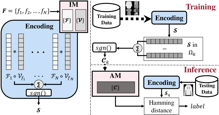
Figure 1. A brain-inspired HDC classifier. IM: item memory. AM: associative memory.

We provide an overview of HDC models as illustrated in Figure 1. Consider an input sample represented as a vector with $N$ features $\mathbf{F}=\{f_{1},f_{2},...,f_{N}\}$, where the value range for each feature is normalized and uniformly discretized into $M$ values, i.e., $f_{i}\in\{1,\cdots,M\}$ for $i=1,\cdots,N$. HDC encodes all the values, features, and samples as hyperdimensional bipolar vectors, e.g., $\mathcal{H}\in\{1,-1\}^{D=10,000}$, which also equivalently correspond to binary 0/1 bits for hardware efficiency (Imani et al., 2019b; Ge and Parhi, 2020). In this paper, we also interchangeably use binary and bipolar if applicable. Note that the input vector $\mathbf{F}=\{f_{1},f_{2},...,f_{N}\}$ can represent raw features or extracted features (using, e.g., neural networks and random feature map (Zou et al., 2021)).

There are four types of hypervectors in HDC models: value hypervector $\mathcal{V}$ (representing the value of a feature), feature hypervector $\mathcal{F}$ (representing the index/position of a feature), sample hypervector $\mathcal{S}$ (representing a training/testing sample), and class hypervector $\mathcal{C}$ (representing a class).

To measure the similarity between two hypervectors, there are two commonly used distances — normalized Hamming and cosine, which are mutually equivalent as shown in the appendix. In this paper, we use the normalized Hamming distance defined as $Hamm(\mathcal{H}_{1},\mathcal{H}_{2})=\frac{|\mathcal{H}_{1}\neq\mathcal{H}_{2}|}{D}$. If two hypervectors $\mathcal{H}_{1}$ and $\mathcal{H}_{2}$ have a normalized Hamming distance of 0.5, they are considered orthogonal. In a hyperdimensional space, two randomly-generated hypervectors are almost orthogonal (Karunaratne et al., 2020; Ge and Parhi, 2020).

Generating value and feature hypervectors: In a typical HDC model (Kanerva, 2009; Ge and Parhi, 2020; Salamat et al., 2019), the value and feature hypervectors are randomly generated in advance and remain unchanged throughout the training and inference process. Most commonly, $N$ feature hypervectors $\mathcal{F}$ are randomly generated to keep mutual orthogonality (e.g., randomly sampling in the hyperdimensional space or rotating one random hypervector), whereas $M$ value hypervectors $\mathcal{V}$ are generated to preserve their value correlations (e.g., flipping a certain number of bits from one randomly-generated value hypervector) (Imani et al., 2019b; Ge and Parhi, 2020; Kanerva, 2009). As a result, the Hamming distance between any two feature hypervectors is approximately 0.5, while the Hamming distance between two value hypervectors denoting normalized feature values of $i,j\in\{1,\cdots,M\}$ is $Hamm(\mathcal{V}_{i},\mathcal{V}_{j})\approx\frac{|i-j|}{2(M-1)}$.

Encoding: An input sample is encoded as a sample hypervector by fetching the pre-generated value and feature hypervectors from the item memory (IM). Specifically, by combining each feature hypervector with its corresponding value hypervector, the encoding output for an input sample is given by

(1) $$\mathcal{S}=sgn\left(\sum^{N}_{i=1}\mathcal{F}_{i}\circ\mathcal{V}_{f_{i}}\right),$$

where $f_{i}$ is the $i$-th feature value, $\mathcal{V}_{f_{i}}$ is the corresponding value hypervector, $\circ$ is the Hadamard product, and $sgn(\cdot)$ is the sign function that binarizes the encoded sample hypervector. As a tiebreaker, we set $sgn(0)=1$.

Training: Given $K$ classes, the training process is to obtain $K$ class hypervectors, each for one class. The basic training process is to simply average the sample hypervectors within a class:

(2) $$\mathcal{C}_{k}=sgn\left(\sum_{\mathcal{S}\in\Omega_{k}}\mathcal{S}\right)$$

where $\Omega_{k}$ is the set of sample hypervectors in $k$-th class. All the class hypervectors are stored in the associative memory (AM).

More recently, to improve the accuracy, SOTA HDC models have also added re-training as part of the training process (Imani et al., 2019a; Ge and Parhi, 2020). Concretely, re-training fine tunes the class hypervectors $\mathcal{C}$ derived in Equation (2): if a training sample is mis-classified, it will be given more weights in correct class hypervector and subtracted from the wrong class hypervector. Essentially, re-training will lead to an adjusted centroid for each class.

Inference: The testing input sample is first encoded in the same way as encoding a training sample. To be distinguished from the training sample hypervector, the testing sample hypervector is also referred to as a query hypervector. For inference, the query hypervector $\mathcal{S}_{q}$ is compared with all the class hypervectors fetched from the associative memory. The most similar one with the lowest Hamming distance indicates the classification result:

(3) $${\arg\min_{k}}\ Hamm(\mathcal{S}_{q},\mathcal{C}_{k}).$$

Due to the equivalence of Hamming distance and cosine similarity (appendix), the classification rule in Equation (3) is equivalent to

(4) $${\arg\max_{k}}\ \mathcal{S}_{q}^{T}\mathcal{C}_{k},$$

which essentially transforms the bit-wise comparison to vector multiplication and is instrumental for establishing the equivalence between an HDC model and a neural network.

3. The Design of LDC Classifiers

In this section, we describe the LDC classifier design which exploits hardware-friendly association of low-dimensional vectors for efficient inference. Specifically, like in its HDC counterpart, our LDC classifier mimics brain cognition for hardware efficiency by representing features using vectors and performing inference via vector association (Kanerva, 2009; Ge and Parhi, 2020). Nonetheless, the existing HDC models rely on randomly-generated hypervectors, which not only limits the accuracy but also results in a large inference latency and resource consumption beyond the capability of tiny devices. Our LDC classifier fundamentally differs from them — it uses vectors with orders-of-magnitude smaller dimensions and optimizes the vectors using a principled approach.

With a slight abuse of notations, we keep using $\mathcal{F}$ and $\mathcal{V}$ to denote feature and value vectors, respectively, in our LDC classifier wherever applicable. But, unlike in an HDC model that has the same hyperdimension of $D$ for all hypervectors, $\mathcal{F}$ and $\mathcal{V}$ can have different and much lower dimensions of $D_{\mathcal{F}}$ and $D_{\mathcal{V}}$, respectively.

3.1. Mapping to a Neural Network

We now divide the LDC classification process into two parts — encoding and similarity checking — and map them to equivalent neural network operation.

3.1.1. Encoding

The encoding process shown in Equation (1) binarizes the summed bindings of value vectors and feature vectors. Instead of using random vectors as in the existing HDC models, we explicitly optimize the value and feature vectors by representing the encoder as a neural network and then using a principled training process. Next, we describe the equivalence between the encoder and its neural network counterpart.

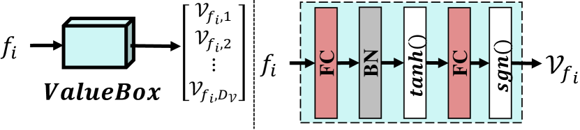
Figure 2. Value mapping. As an example, we use a 2-layer fully connected network as the ValueBox. FC: fully-connected, BN: batch normalization.

Value mapping: As shown in Figure 2, $\mathcal{V}_{f_{i}}$ represents a discretized feature value $f_{i}\in\{1,\cdots,M\}$ with a certain (bipolar) vector. For the ease of presentation, we refer to this mapping functionality as ValueBox. In an HDC model, ValueBox essentially assigns a random hypervector to a feature value. Alternatively, one may manually design a ValueBox, e.g., representing a value directly using its binary code (say, $9\to\texttt{1001}$) (Zhang et al., 2021). In our LDC design, however, we exploit the strong representation power of neural networks and use a trainable neural network for the ValueBox. For example, Figure 2 illustrates a simple fully-connected neural network with $tanh$ activation to map a value $f_{i}$ to a binary value vector $\mathcal{V}_{f_{i}}$. We will jointly train the ValueBox network together with subsequent operators to optimize the inference accuracy.

Element-wise binding: As shown in Equation (1), the encoder binds the feature and value vectors using a Hadamard product. Nonetheless, in our LDC classifier, we do not require $D_{\mathcal{F}}=D_{\mathcal{V}}$, which makes the Hadamard product inapplicable. Here, we set $D_{\mathcal{F}}$ as an integer multiple of $D_{\mathcal{V}}$, i.e., $D_{\mathcal{F}}/D_{\mathcal{V}}=n$, for $n\in\mathbb{N}^{+}$. As a result, a value vector $\mathcal{V}_{f_{i}}$ can be stacked for $n$ times in order to have the same dimension as its corresponding feature vector $\mathcal{F}_{i}$ for Hadamard product. Equivalently, a feature vector can be evenly divided into $n$ parts or sub-vectors, each aligned with the value vector for Hadamard product. Thus, the binding for the $i$-th feature vector and its corresponding value vector can be represented as

(5) $$\begin{bmatrix}\mathcal{F}_{i}^{1}\circ\mathcal{V}_{f_{i}}\\ ...\\ \mathcal{F}_{i}^{n}\circ\mathcal{V}_{f_{i}}\end{bmatrix}=\begin{bmatrix}diag(\mathcal{F}_{i}^{1})\\ ...\\ diag(\mathcal{F}_{i}^{n})\end{bmatrix}\mathcal{V}_{f_{i}}.$$

Through element-wise binding, the encoder outputs a sample vector given by

(6) $$\mathcal{S}=sgn\left(\sum_{i=1}^{N}\begin{bmatrix}diag(\mathcal{F}_{i}^{1})\\ ...\\ diag(\mathcal{F}_{i}^{n})\end{bmatrix}\mathcal{V}_{f_{i}}\right).$$

Crucially, the element-wise binding used by the encoder is equivalently mapped to matrix multiplication in Equation (6). Therefore, it can be represented as a simple BNN whose architecture is shown in Figure 3 and referred to as a feature layer. Specifically, by stacking $N$ value vectors $\mathcal{V}_{f_{i}}$ for $i=1,\cdots,N$, the input to the feature layer is a vector with $ND_{\mathcal{V}}$ elements. Also, the structurally sparse weight matrix $\mathbf{\Theta}$ in the feature layer is the collection of feature vectors $\mathcal{F}_{i}$ for $i=1,\cdots,N$, with only $ND_{\mathcal{F}}$ bipolar elements in total. By transforming the encoder into an equivalent BNN, we can leverage a principled training process (described in Section 3.2) to optimize the weight matrix $\mathbf{\Theta}$, which in turn leads to optimized feature vectors $\mathcal{F}_{i}$ with a small dimension instead of random hypervectors used by the existing HDC models.

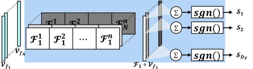
Figure 3. Illustration of a feature layer that binds value and feature vectors.

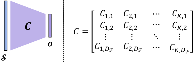
Figure 4. Illustration of a class layer.

3.1.2. Similarity Checking

In our LDC classifier, the classification process involves checking the similarities between a query hypervector and all class hypervectors. Specifically, as shown in Equations (3) and (4), the similarity check is equivalent to matrix calculation, which can also be mapped to the operation in a BNN. Hence, we transform Equation (4) into a class layer as shown in Figure 4. The input to the class layer is the sample vector, which is also the output of the preceding feature layer. The weight of the class layer is a $D_{\mathcal{F}}\times K$ matrix that represents the collection of all the class vectors $\mathcal{C}_{k}$ for $k=1,\cdots,K$. The output of the class layer includes $K$ products, and class $k$ with the maximum product $\mathcal{S}^{T}\mathcal{C}_{k}$ is chosen as the classification result.

3.1.3. End-to-end mapping.

By integrating different stages of the LDC classification pipeline, we now construct an end-to-end neural network shown in Figure 5. With both non-binary and binary weights, the neural network achieves the same function as our LDC classifier, and this equivalence allows a principled training approach to optimize the weights.

Specifically, in the equivalent neural network, each of the $N$ feature values of an input sample is first fed to a ValueBox, which is a non-binary neural network and outputs bipolar value vectors. Note that a single ValueBox is shared by all features to keep the model size small, while our design can easily generalize to different ValueBoxes for different features at the expense of increasing the model size (in particular, the size of item memory). Then, the $N$ value vectors enter a feature layer, which is a structurally sparse BNN as described in Section 3.1.1 and outputs a sample vector. Finally, the sample vector goes through a class layer, based on which we can decide the classification result.

SOTA HDC models: Besides the obvious drawback of ultra-high dimension, we can clearly see another major drawback by casting an existing HDC model into our equivalent neural network. Concretely, the ValueBox outputs and the feature layer weights corresponding to an HDC model are essentially randomly generated, and even the weights in the class layer (i.e., $K$ class hypervectors in an HDC model) are obtained by using simple averaging methods in conjunction with heuristic re-training (Ge and Parhi, 2020; Kanerva, 2009; Imani et al., 2019b). Thus, the inference accuracy in the existing HDC models are highly sub-optimal.

3.2. Training LDC Classifiers

To address the fundamental drawbacks of existing HDC models and maximize the accuracy with a much smaller model size, we can optimize the weights in its equivalent neural network that has both non-binary weights (in the ValueBox) and binary weights (in the feature layer and class layer). Specifically, following SOTA training methods for BNNs (Liu et al., 2021), we use Adam with weight decay as the optimization method and consider softmax activation with CrossEntropy as the loss function. Due to the equivalence of Hamming distance and cosine similarity metrics for binary vectors, classification based on the largest softmax probability (or equivalently, ${\arg\max_{k}}\mathcal{S}_{q}^{T}\mathcal{C}_{k}$) is equivalent to classification based on the minimum normalized Hamming distance. Additionally, while CrossEntropy is commonly used for classification tasks, we can also use other loss functions such as hinge loss (Goodfellow et al., 2016). For training, we set the learning rate by starting with a large value (such as 0.001) with decaying linearly.

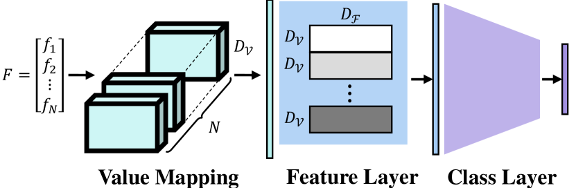
Figure 5. Mapping an LDC classifier to a neural network.

After training, the vectors used in our LDC classifier can be extracted as follows for testing.

The value vectors $\mathcal{V}$ can be extracted from the ValueBox by recording the output corresponding to each possible input. For example, the value vector ($\mathcal{V}_{f}$) for a certain feature value $f$ is $ValueBox(f)$. Due to $D_{\mathcal{F}}/D_{\mathcal{V}}=n$ for Hadamard product, the value vector is stacked $n$ times in the encoder to align with the dimension of feature vectors. Thus, the non-binary weights in the ValueBox are not utilized for inference and can be discarded once the value vectors are extracted.

The feature vectors $\mathcal{F}$ are extracted from the weight matrix in the feature layer. For the $i$-th feature, the feature vector $\mathcal{F}_{i}$ can be extracted from the corresponding values in the $i$-th weight matrix block:

$$\begin{bmatrix}\mathcal{F}_{i,1}^{1}&0&...&0&\cdots&\mathcal{F}_{i,1}^{n}&0&...&0\\ 0&\mathcal{F}_{i,2}^{1}&...&0&\cdots&0&\mathcal{F}_{i,2}^{n}&...&0\\ \vdots&\vdots&\ddots&\vdots&\cdots&\vdots&\vdots&\ddots&\vdots\\ 0&0&...&\mathcal{F}_{i,D_{\mathcal{V}}}^{1}&\cdots&0&0&...&\mathcal{F}_{i,D_{\mathcal{V}}}^{n}\end{bmatrix}$$

such that $\mathcal{F}_{i}$ is composed of $[\mathcal{F}_{i}^{1},\mathcal{F}_{i}^{2},\cdots,\mathcal{F}_{i}^{n}]$ with dimension $D_{\mathcal{F}}$, where $\mathcal{F}_{i}^{j}=[\mathcal{F}_{i,1}^{j},\cdots,\mathcal{F}_{i,D_{\mathcal{V}}}^{j}]$ for $j=1,2,\cdots,n$.

As shown in the right side of Figure 4, the class vectors $\mathcal{C}$ can be directly extracted from the weight matrix in class layer.

Like in Figure 1, the extracted value and feature vectors are stored in the item memory for encoding, and the class vectors are stored in the associative memory for similarity checking.

3.3. Inference

For inference, our LDC classifier still follows the encoding and similarity checking process as described in Section 2. Specifically, each feature value of an input sample is first mapped to a value vector, which is then combined together with the corresponding feature vector to form a query sample vector. The query vector is compared with the class vectors for similarity checking and yielding the classification results. In most BNNs, the fully-connected layers still use non-binary weights, which can slow down the inference process on tiny devices (Zhang et al., 2021). By contrast, although the offline training process involves non-binary weights in the ValueBox neural network, the inference process of our LDC classifier is fully binary by utilizing bit-wise operation and association for classification.

4. Performance Evaluation

In this section, we evaluate the performance of our LDC classifier on different datasets and highlight that it offers an overwhelming advantage over the SOTA HDC models: better accuracy and orders-of-magnitude smaller dimension.

4.1. Experimental Setup

Like in the existing HDC research (Imani et al., 2019b; Ge and Parhi, 2020), we select four application scenarios for inference on tiny devices: computer vision (MNIST (LeCun et al., 1998) and Fashion-MNSIT (Xiao et al., 2017)), human activity (UCIHAR (Anguita et al., 2013)), voice recognition (ISOLET (Cole and Fanty, 1994)), and cardiotocography (CTG (de Sa et al., 2010)). Each feature value is normalized to $[0,255]$ and quantized to an 8-bit integer. The configurations for each dataset is shown in Table 1. We compare LDC with the SOTA HDC model with re-training (Imani et al., 2019a), and the basic HDC model without re-training (Ge and Parhi, 2020). As reported in (Imani et al., 2019a), the HDC accuracy has significant reduction when the hypervector dimension is lower than $8,000$. Thus, we use $D=8,000$ for both SOTA and basic HDC. For training, all the experiments are executed in Python with Tesla V100 GPU. For the inference, we also build a hardware acceleration platform on a Zynq UltraScale+ ZU3EG FPGA embedded on the Ultra96 evaluation board.

4.2. Hyperparameter Selection

4.2.1. Value mapping

We test different neural networks for the ValueBox and also compare them against two manual designs (i.e., fix-point encoding and thermometer encoding (Zhang et al., 2021), as illustrated in Figure 6). We set $D_{\mathcal{V}}=8$ to make fix-point encoding and thermometer encoding capable of representing 256 values. Considering the Fasion-MNIST dataset, we see that our neural networks can discover better ValueBoxes than manual designs to achieve higher accuracy. On the other hand, it has no significant differences by varying the network size, such as $1\times 10\times D_{\mathcal{V}}$ vs. $1\times 20\times D_{\mathcal{V}}$. In our experiments, we will use $1\times 20\times D_{\mathcal{V}}$ for the neural network in the ValueBox.

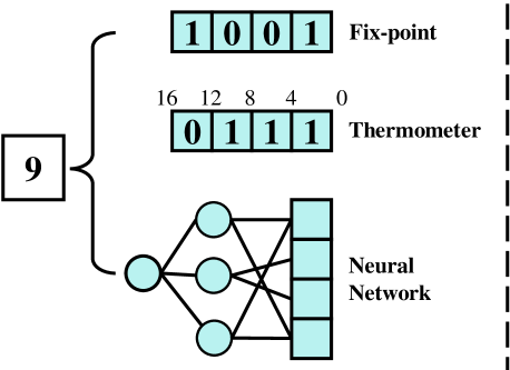
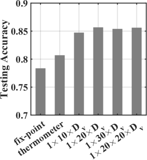
Figure 6. Different ValueBoxes. The testing accuracies are presented on the right side with Fashion-MNIST (Xiao et al., 2017).

4.2.2. Dimensions

The dimensions $D_{\mathcal{V}}$ and $D_{\mathcal{F}}$ used in our LDC classifier are important hyperparameters. As a case study, we use Fashion-MNIST to evaluate the impact of $D_{\mathcal{V}}$ and $D_{\mathcal{F}}$ on the accuracy. By setting different $n=D_{\mathcal{F}}/D_{\mathcal{V}}$, we also vary $D_{\mathcal{V}}=2,4,8,16$, as presented in Figure 7. In general, a higher $D_{\mathcal{V}}$ retains richer information about the input, thus yielding a higher accuracy. Nonetheless, even with $D_{\mathcal{V}}=2$ or $D_{\mathcal{V}}=4$, we can still achieve a reasonably good accuracy by increasing $D_{\mathcal{F}}$. In all cases, our dimensions are orders-of-magnitude smaller than the dimensions of 8,000 or higher in existing HDC models.

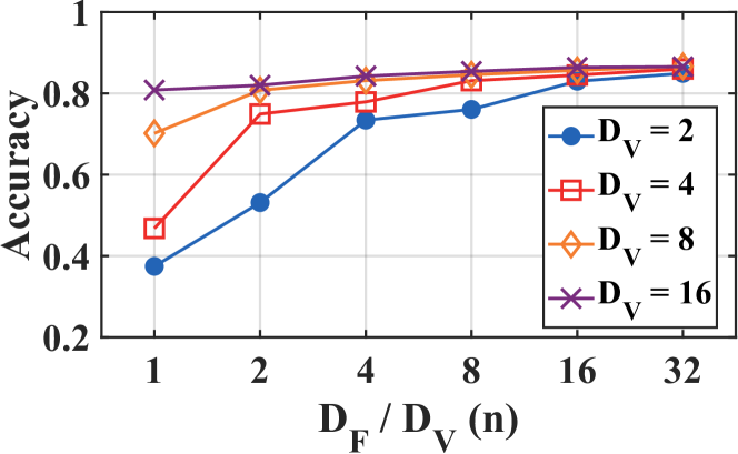
Figure 7. The inference accuracy with different $D_{\mathcal{V}}$ and $D_{\mathcal{F}}$ on Fashion-MNIST. Initial learning rate is $1\times 10^{-3}$, weight decay is $1\times 10^{-4}$, and learning rate will decay by half every 5 iterations.

Table 1. Configuration of our LDC classifier for each dataset. The batch size is 64.

Dataset	N	# of (train, test, class)	$D_{\mathcal{V}}$, $D_{\mathcal{F}}$	LR1	WD2
MNIST	784	(60000, 10000, 10)	4, 64	0.0001	0
Fashion-MNIST	784	(60000, 10000, 10)	4, 64	0.0002	0.00001
UCIHAR	561	(7352, 2947, 6)	4, 128	0.001	0.0001
ISOLET	617	(6328, 1559, 26)	4, 128	0.005	0.0001
CTG	21	(1701, 425, 3)	4, 64	0.008	0.0001
1 LR = Learning Rate 2 WD = Weight Decay

4.3. Inference Accuracy

In Table 2, we evaluate the inference accuracy that LDC can achieve compared to both basic and SOTA HDC models. The result shows that LDC can outperform existing HDC models that use random value/feature vectors and heuristically generate class vectors. While retraining improves the inference accuracy against the basic HDC, the hypervector dimension must be as large as 8,000 to prevent accuracy degradation. By contrast, our LDC classifier reduces the dimension significantly, without introducing any extra cost during the inference process.

Table 2. Inference accuracy (%, in $mean^{\pm std}$).

Classifier	MNIST	Fashion-MNIST	UCIHAR	ISOLET	CTG
LDC	$\textbf{92.72}^{\pm 0.18}$	$\textbf{85.47}^{\pm 0.29}$	$\textbf{92.56}^{\pm 0.41}$	$\textbf{91.33}^{\pm 0.50}$	$\textbf{90.50}^{\pm 0.46}$
Basic HDC	$79.35^{\pm 0.03}$	$69.11^{\pm 0.03}$	$89.17^{\pm 0.16}$	$85.90^{\pm 0.25}$	$71.35^{\pm 0.76}$
SOTA HDC (Imani et al., 2019a)	$87.38^{\pm 0.21}$	$79.24^{\pm 0.52}$	$90.31^{\pm 0.06}$	$90.66^{\pm 0.31}$	$89.51^{\pm 0.43}$

Table 3. Hardware acceleration on inference with two selected datasets. The system frequency is 200MHz.

Dataset	Name	Accuracy (%)	Platform	Model Size (KB)	Latency ($\mu$s)	(LUT, BRAM, DSP)	Energy (nJ)
MNIST	LDC	92.72	Zynq UltraScale+	6.48	3.99	(745, 5, 1)	64
	SOTA HDC	87.38	Zynq UltraScale+	1050	499	(768, 178, 1)	36926
	FINN (Umuroglu et al., 2017)	95.83	Zynq-7000	600	240	(5155, 16, -)	96000
CTG	LDC	90.50	Zynq UltraScale+	0.32	0.14	(345, 3, 1)	0.945
	SOTA HDC	89.51	Zynq UltraScale+	280	16.88	(362, 9, 1)	169
	Compressed HDC (Basaklar et al., 2021)	$\sim$82	Odroid XU3	45.1	90	NA	6300

4.4. Hardware Acceleration

4.4.1. Hardware design

For hardware implementation, bipolar values $\{1,-1\}$ are represented as binary values $\{0,1\}$, respectively. The multiplication and accumulation on bipolar values are realized using XOR and popcount which is constructed using tree adders, on the binary representation (Liang et al., 2018).

The existing HDC models typically exploit full parallelism for acceleration. For example, given $N$ features, the FPGA prepares $N$ identical hypervector multiplication blocks to encode all the features simultaneously, incurring a high resource expenditure (e.g., over $10^{5}$ LUTs, 100 BRAMs, and 800 DSPs in SOTA FPGA acceleration (Imani et al., 2021)). Nonetheless, this design does not fit into tiny devices, for which we must limit the resource utilization.

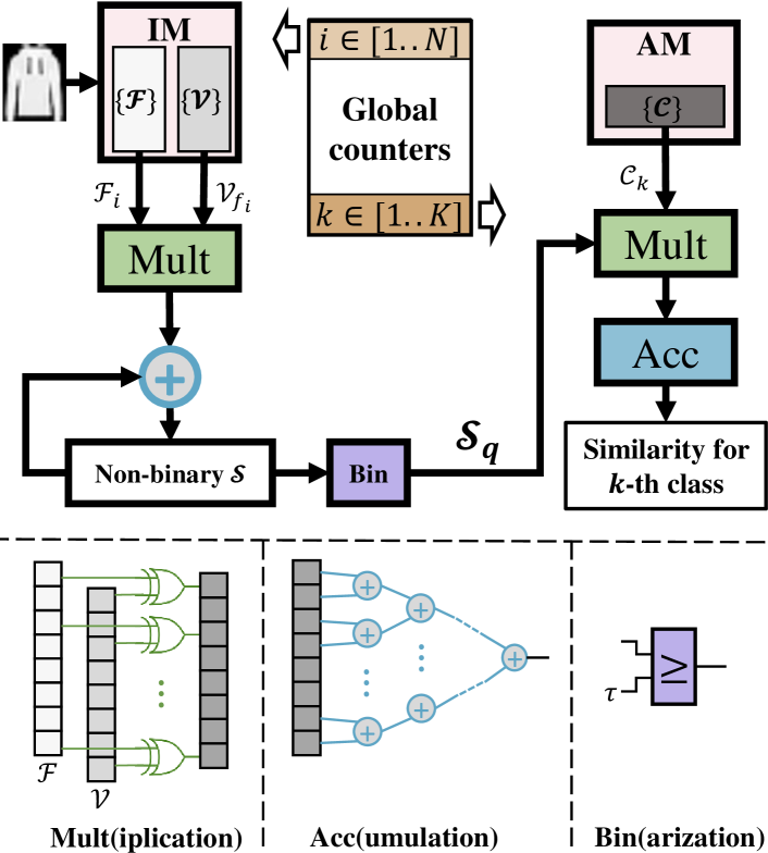
Figure 8. The hardware acceleration for LDC on FPGA. IM: Item Memory. AM: Associative Memory.

We design a pipeline structure for feature encoding, rather than in parallel, to fit into tiny devices. The structure is demonstrated in Figure 8. Only one vector multiplication block and several BRAMs are required. Although the encoding time will increase to $N+1$ cycles, the latency is still on a microsecond scale. Subsequently, one adder is utilized to accumulate the multiplied vectors, followed by a threshold ($\tau=N/2$) comparator to binarize the encoding output. For checking similarity, we also use a pipeline structure for comparison on all class vectors. Then, a tree adder along the vector dimension is used for Hamming distance calculation. Finally, we transfer the Hamming distances back to the CPU to execute the $\arg\min()$ function for classification.

4.4.2. Results

In Table 3, we show the efficiency results. As we focus on tiny devices, we limit the resource utilization, e.g., $<1$MB model size and $<10$k LUT utilization. To evaluate the existing HDC models, for fair comparison, we also implement the SOTA HDC classifier (Imani et al., 2019a) with $D=8,000$ using our acceleration designs. Moreover, we choose two other lightweight models for comparison: a compressed HDC model (Basaklar et al., 2021) that uses a small vector but has non-binary weights and per-feature ValueBoxes founded using evolutionary search; and SFC-fix with FINN (Umuroglu et al., 2017) that applies a 3-layer binary MLP on FPGA. For these models, we only report their results available for our considered datasets. Like in the literature (Imani et al., 2021, 2019a), the results are measured for model inference only, excluding data transmission between the FPGA and CPU.

For the MNIST dataset, by reducing the dimension of SOTA HDC models by $125$ times, the model size of LDC is only 6.48 KB. Further, the low dimension can benefit the resource utilization and execution time. For the SOTA HDC model with $D=8,000$, the number of BRAMs increases greatly to store all hypervectors, but other resources such as LUT and DSP do not increase dramatically due to sequential execution to account for tiny devices; consequently, the latency increases by $125$ times. For energy consumption, the result shows that our LDC classifier has the lowest, because of the very low resource utilization and short latency. For the CTG dataset, the results are even more impressive as shown in Table 3.

4.5. Robustness Against Random Bit Errors

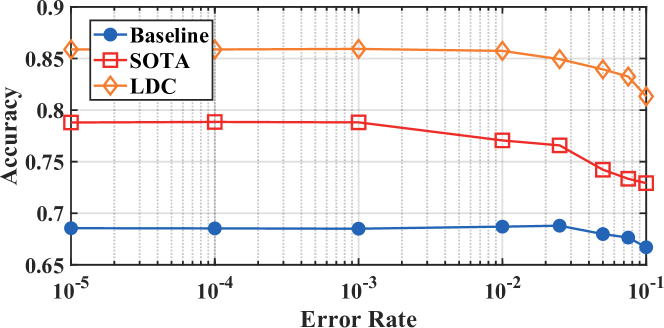
Figure 9. Bit error robustness of different models for Fashion-MNIST dataset. The accuracy is averaged over five different runs for each case.

While inefficient, a natural byproduct of the hyperdimensionality of HDC classifiers is the robustness against random hardware bit errors (Podual et al., 2021; Ma et al., 2021). By contrast, our LDC classifier reduces the dimension by orders of magnitude and hence might become less robust against random bit errors. Here, we show in Figure 9 the robustness analysis for both LDC and HDC classifiers. Specifically, we inject bit errors in the associative memory under various bit error rates, and assess the inference accuracy caused by the injected bit errors. We see that our LDC classifier has the highest accuracy and also achieves comparable robustness on a par with the HDC counterparts. The counter-intuitive results can be explained by the fact that, although our LDC classifier significantly reduces dimensions, the information is still spread uniformly within each compact vector (i.e., different bits are equally important), thus exhibiting robustness against random bit errors.

Note finally that we can also run multiple LDC classifiers and apply the majority rule for better robustness. Due to the orders-of-magnitude dimension reduction, the total size of multiple LDC classifiers is still much less than that of a single HDC classifier.

5. Related Work

The set of applications with HDC classifiers have been proliferating, include language classification (Imani et al., 2017), image classification (Ge and Parhi, 2020; Chang et al., 2020), emotion recognition based on physiological signals (Chang et al., 2019), distributed fault isolation in power plants (Kleyko et al., 2018), gesture recognition for wearable devices (Benatti et al., 2019), seizure onset detection (Burrello et al., 2020), and robot navigation (Mitrokhin et al., 2019).

Nonetheless, the training process for existing HDC classifiers is mostly heuristics-driven and often relies on random hypervectors for encoding, resulting in low inference accuracy (Ge and Parhi, 2020). In many cases, even a well-defined loss function is lacking for training HDC classifiers. More recently, (Ganesan et al., 2021) learns a neural network model based on non-binary hypervector representations, and (Diao et al., 2021) uses generalized learning vector quantization (GLVQ) to optimize the class vectors. But, they both consider hyperdimensional representations based on random hypervectors, thus resulting in an overly large model size.

In addition, the ultra-high dimension is another fundamental drawback of HDC models. Simply reducing the dimension without fundamentally changing the HDC design can dramatically decrease the inference accuracy A recent study (Basaklar et al., 2021) reduces the dimension but considers non-binary HDC that is unfriendly to hardware acceleration. Moreover, it uses different sets of value vectors for different features, and hence results in a large model size (Table 3). Last but not least, its training process is still heuristic-driven as in the existing HDC models. By sharp contrast, our LDC classifier is optimized based on a principled training approach guided by a loss function, and offers an overwhelming advantage over the existing HDC models, in terms of accuracy, model size, inference latency, and energy consumption.

Our LDC classifier is relevant to but also differs significantly from BNNs which use binary weights to speed up inference (Zhang et al., 2021; Rastegari et al., 2016; Yuan and Agaian, 2021). To avoid information loss, non-binary weights are still utilized in the early stage of typical BNNs (Rastegari et al., 2016; Yuan and Agaian, 2021) which may not be supported by tiny devices, whereas the inference of our LDC classifier is fully binary and follows a brain-like cognition process. More recently, (Zhang et al., 2021) manually designs the value mapping from raw features to binary features. In our design, we use a neural network to automatically learn the mapping which, as shown in Figure 6, outperforms manual designs in terms of accuracy.

6. Conclusion

In this paper, we address the fundamental drawbacks of existing HDC models and propose an LDC alternative. We map our LDC classifier into an equivalent neural network, and optimize the model using a principled training approach. We run experiments to evaluate our LDC classifier, and also implement different models on an FPGA platform for acceleration. The results highlight that our LDC classifier has an overwhelming advantage over the existing HDC models and is particularly suitable for inference on tiny devices.

Appendix

We show the equivalence between the (normalized) Hamming distance and cosine similarity on two bipolar vectors. The normalized Hamming distance and cosine similarity are defined as: $Hamm(\mathcal{H}_{1},\mathcal{H}_{2})=\frac{|\mathcal{H}_{1}\neq\mathcal{H}_{2}|}{D}$, and $cosine(\mathcal{H}_{1},\mathcal{H}_{2})=\frac{\mathcal{H}_{1}^{T}\mathcal{H}_{2}}{\|\mathcal{H}_{1}\|\ \|\mathcal{H}_{2}\|}$, where $|\mathcal{H}_{1}\neq\mathcal{H}_{2}|$ denotes the number of different bits in $\mathcal{H}_{1}$ and $\mathcal{H}_{2}$, $\|\mathcal{H}_{1}\|$ and $\|\mathcal{H}_{2}\|$ denote the $l_{2}$ norms of $\mathcal{H}_{1}$ and $\mathcal{H}_{2}$, respectively. Since vectors are in bipolar $\{1,-1\}$, we have $\mathcal{H}_{1}^{T}\mathcal{H}_{2}=(|\mathcal{H}_{1}=\mathcal{H}_{2}|-|\mathcal{H}_{1}\neq\mathcal{H}_{2}|)$. Plus the fact that $\|\mathcal{H}_{1}\|\ \|\mathcal{H}_{2}\|=D$ and $(|\mathcal{H}_{1}\neq\mathcal{H}_{2}|+|\mathcal{H}_{1}=\mathcal{H}_{2}|)=D$, we can conclude $cosine(\mathcal{H}_{1},\mathcal{H}_{2})=\frac{D-2|\mathcal{H}_{1}\neq\mathcal{H}_{2}|}{D}=1-2Hamm(\mathcal{H}_{1},\mathcal{H}_{2})$.

References

- (1)
- Anguita et al. (2013) Davide Anguita, Alessandro Ghio, Luca Oneto, Xavier Parra, Jorge Luis Reyes-Ortiz, et al. 2013. A public domain dataset for human activity recognition using smartphones.. In Esann, Vol. 3. 3.
- Basaklar et al. (2021) Toygun Basaklar, Yigit Tuncel, Shruti Yadav Narayana, Suat Gumussoy, and Umit Y Ogras. 2021. Hypervector Design for Efficient Hyperdimensional Computing on Edge Devices. arXiv preprint arXiv:2103.06709 (2021).
- Benatti et al. (2019) Simone Benatti, Fabio Montagna, Victor Kartsch, Abbas Rahimi, Davide Rossi, and Luca Benini. 2019. Online Learning and Classification of EMG-Based Gestures on a Parallel Ultra-Low Power Platform Using Hyperdimensional Computing. IEEE Transactions on Biomedical Circuits and Systems 13, 3 (2019), 516–528.
- Burrello et al. (2020) Alessio Burrello, Kaspar Schindler, Luca Benini, and Abbas Rahimi. 2020. Hyperdimensional Computing With Local Binary Patterns: One-Shot Learning of Seizure Onset and Identification of Ictogenic Brain Regions Using Short-Time iEEG Recordings. IEEE Transactions on Biomedical Engineering 67, 2 (2020), 601–613.
- Chang et al. (2020) Cheng-Yang Chang, Yu-Chuan Chuang, and An-Yeu (Andy) Wu. 2020. Task-Projected Hyperdimensional Computing for Multi-task Learning. In Artificial Intelligence Applications and Innovations.
- Chang et al. (2019) En-Jui Chang, Abbas Rahimi, Luca Benini, and An-Yeu Andy Wu. 2019. Hyperdimensional Computing-based Multimodality Emotion Recognition with Physiological Signals. In IEEE International Conference on Artificial Intelligence Circuits and Systems.
- Cole and Fanty (1994) Ron Cole and Mark Fanty. 1994. ISOLET. UCI Machine Learning Repository.
- de Sa et al. (2010) J P Marques de Sa, J Bernardes, and D Ayres de Campos. 2010. Cardiotocography. UCI Machine Learning Repository.
- Diao et al. (2021) Cameron Diao, Denis Kleyko, Jan M. Rabaey, and Bruno A. Olshausen. 2021. Generalized Learning Vector Quantization for Classification in Randomized Neural Networks and Hyperdimensional Computing. arXiv:2106.09821 [cs.LG]
- Ganesan et al. (2021) Ashwinkumar Ganesan, Hang Gao, Sunil Gandhi, Edward Raff, Tim Oates, James Holt, and Mark McLean. 2021. Learning with Holographic Reduced Representations. In Advances in Neural Information Processing Systems, A. Beygelzimer, Y. Dauphin, P. Liang, and J. Wortman Vaughan (Eds.). https://openreview.net/forum?id=RX6PrcpXP-
- Ge and Parhi (2020) Lulu Ge and Keshab K. Parhi. 2020. Classification Using Hyperdimensional Computing: A Review. IEEE Circuits and Systems Magazine 20, 2 (2020), 30–47.
- Goodfellow et al. (2016) Ian Goodfellow, Yoshua Bengio, and Aaron Courville. 2016. Deep Learning. MIT Press. http://www.deeplearningbook.org.
- Han et al. (2016) Song Han, Huizi Mao, and William J. Dally. 2016. Deep Compression: Compressing Deep Neural Networks with Pruning, Trained Quantization and Huffman Coding. In ICLR.
- Huang et al. (2014) Longbo Huang, Xin Liu, and Xiaohong Hao. 2014. The Power of Online Learning in Stochastic Network Optimization. In The 2014 ACM International Conference on Measurement and Modeling of Computer Systems (Austin, Texas, USA) (SIGMETRICS ’14). Association for Computing Machinery, New York, NY, USA, 153–165. https://doi.org/10.1145/2591971.2591990
- Imani et al. (2019a) Mohsen Imani, Samuel Bosch, Sohum Datta, Sharadhi Ramakrishna, Sahand Salamat, Jan M Rabaey, and Tajana Rosing. 2019a. QuantHD: A quantization framework for hyperdimensional computing. IEEE Transactions on Computer-Aided Design of Integrated Circuits and Systems (2019).
- Imani et al. (2017) Mohsen Imani, John Hwang, Tajana Rosing, Abbas Rahimi, and Jan M Rabaey. 2017. Low-Power Sparse Hyperdimensional Encoder for Language Recognition. IEEE Design Test 34, 6 (2017), 94–101.
- Imani et al. (2019b) Mohsen Imani, John Messerly, Fan Wu, Wang Pi, and Tajana Rosing. 2019b. A Binary Learning Framework for Hyperdimensional Computing. In DATE.
- Imani et al. (2019c) Mohsen Imani, Xunzhao Yin, John Messerly, Saransh Gupta, Michael Niemier, Xiaobo Sharon Hu, and Tajana Rosing. 2019c. Searchd: A memory-centric hyperdimensional computing with stochastic training. IEEE Transactions on Computer-Aided Design of Integrated Circuits and Systems 39, 10 (2019), 2422–2433.
- Imani et al. (2021) Mohsen Imani, Zhuowen Zou, Samuel Bosch, Sanjay Anantha Rao, Sahand Salamat, Venkatesh Kumar, Yeseong Kim, and Tajana Rosing. 2021. Revisiting hyperdimensional learning for fpga and low-power architectures. In 2021 IEEE International Symposium on High-Performance Computer Architecture (HPCA). IEEE, 221–234.
- Kanerva (2009) Pentti Kanerva. 2009. Hyperdimensional computing: An introduction to computing in distributed representation with high-dimensional random vectors. Cognitive computation 1, 2 (2009), 139–159.
- Karunaratne et al. (2020) Geethan Karunaratne, Manuel Le Gallo, Giovanni Cherubini, Luca Benini, Abbas Rahimi, and Abu Sebastian. 2020. In-memory Hyperdimensional Computing. Nature Electronics (Jun 2020).
- Kleyko et al. (2019) Denis Kleyko, Mansour Kheffache, E. Paxon Frady, Urban Wiklund, and Evgeny Osipov. 2019. Density Encoding Enables Resource-Efficient Randomly Connected Neural Networks. arXiv preprint arXiv:1909.09153 (2019).
- Kleyko et al. (2018) Denis Kleyko, Evgeny Osipov, Nikolaos Papakonstantinou, and Valeriy Vyatkin. 2018. Hyperdimensional Computing in Industrial Systems: The Use-case of Distributed Fault Isolation in a Power Plant. IEEE Access 6 (May 2018), 30766–30777.
- LeCun et al. (1998) Yann LeCun, Léon Bottou, Yoshua Bengio, and Patrick Haffner. 1998. Gradient-based learning applied to document recognition. Proc. IEEE 86, 11 (1998), 2278–2324. https://doi.org/10.1109/5.726791
- Li et al. (2021) Chaojian Li, Zhongzhi Yu, Yonggan Fu, Yongan Zhang, Yang Zhao, Haoran You, Qixuan Yu, Yue Wang, Cong Hao, and Yingyan Lin. 2021. HW-NAS-Bench: Hardware-Aware Neural Architecture Search Benchmark. In ICLR. https://openreview.net/forum?id=_0kaDkv3dVf
- Liang et al. (2018) Shuang Liang, Shouyi Yin, Leibo Liu, Wayne Luk, and Shaojun Wei. 2018. FP-BNN: Binarized neural network on FPGA. Neurocomputing 275 (2018), 1072–1086.
- Lin et al. (2020) Ji Lin, Wei-Ming Chen, Yujun Lin, john cohn, Chuang Gan, and Song Han. 2020. MCUNet: Tiny Deep Learning on IoT Devices. In NeurIPS.
- Liu et al. (2021) Zechun Liu, Zhiqiang Shen, Shichao Li, Koen Helwegen, Dong Huang, and Kwang-Ting Cheng. 2021. How Do Adam and Training Strategies Help BNNs Optimization? arXiv preprint arXiv:2106.11309 (2021).
- Ma et al. (2021) Dongning Ma, Jianmin Guo, Yu Jiang, and Xun Jiao. 2021. HDTest: Differential Fuzz Testing of Brain-Inspired Hyperdimensional Computing. In 2021 58th ACM/IEEE Design Automation Conference (DAC). 391–396. https://doi.org/10.1109/DAC18074.2021.9586169
- Mitrokhin et al. (2019) Anton Mitrokhin, P Sutor, Cornelia Fermüller, and Yiannis Aloimonos. 2019. Learning Sensorimotor Control with Neuromorphic Sensors: Toward Hyperdimensional Active Perception. Science Robotics 4, 30 (2019).
- Podual et al. (2021) P. Podual, Y. Ni, Y. Kim, K. Ni, R. Kuma, R. Cammarota, and M. Imani. 2021. Hyperdimensional Self-Learning Systems Robust to Technology Noise and Bit-Flip Attacks. In IEEE/ACM International Conference On Computer Aided Design (ICCAD).
- Rahimi and Recht (2007) Ali Rahimi and Benjamin Recht. 2007. Random Features for Large-Scale Kernel Machines. In Proceedings of the 20th International Conference on Neural Information Processing Systems (Vancouver, British Columbia, Canada) (NIPS’07). Curran Associates Inc., Red Hook, NY, USA, 1177–1184.
- Rastegari et al. (2016) Mohammad Rastegari, Vicente Ordonez, Joseph Redmon, and Ali Farhadi. 2016. XNOR-Net: ImageNet Classification Using Binary Convolutional Neural Networks. In ECCV, Bastian Leibe, Jiri Matas, Nicu Sebe, and Max Welling (Eds.).
- Salamat et al. (2019) Sahand Salamat, Mohsen Imani, Behnam Khaleghi, and Tajana Rosing. 2019. F5-HD: Fast Flexible FPGA-Based Framework for Refreshing Hyperdimensional Computing. In FPGA.
- Umuroglu et al. (2017) Yaman Umuroglu, Nicholas J Fraser, Giulio Gambardella, Michaela Blott, Philip Leong, Magnus Jahre, and Kees Vissers. 2017. Finn: A framework for fast, scalable binarized neural network inference. In Proceedings of the 2017 ACM/SIGDA International Symposium on Field-Programmable Gate Arrays. 65–74.
- Wen et al. (2016) Wei Wen, Chunpeng Wu, Yandan Wang, Yiran Chen, and Hai Li. 2016. Learning Structured Sparsity in Deep Neural Networks. In NIPS.
- Xiao et al. (2017) Han Xiao, Kashif Rasul, and Roland Vollgraf. 2017. Fashion-MNIST: a Novel Image Dataset for Benchmarking Machine Learning Algorithms. arXiv:cs.LG/1708.07747 [cs.LG]
- Yuan and Agaian (2021) Chunyu Yuan and Sos S. Agaian. 2021. A comprehensive review of Binary Neural Network. CoRR abs/2110.06804 (2021).
- Zhang et al. (2021) Yichi Zhang, Junhao Pan, Xinheng Liu, Hongzheng Chen, Deming Chen, and Zhiru Zhang. 2021. FracBNN: Accurate and FPGA-efficient binary neural networks with fractional activations. In The 2021 ACM/SIGDA International Symposium on Field-Programmable Gate Arrays. 171–182.
- Zou et al. (2021) Zhuowen Zou, Yeseong Kim, Farhad Imani, Haleh Alimohamadi, Rosario Cammarota, and Mohsen Imani. 2021. Scalable Edge-Based Hyperdimensional Learning System with Brain-like Neural Adaptation. In Proceedings of the International Conference for High Performance Computing, Networking, Storage and Analysis (St. Louis, Missouri) (SC’21). Article 38, 15 pages.