Max Weight Independent Set in graphs with no long claws: An analog of the Gyárfás’ path argument

Abstract

We revisit recent developments for the Maximum Weight Independent Set problem in graphs excluding a subdivided claw $S_{t,t,t}$ as an induced subgraph [Chudnovsky, Pilipczuk, Pilipczuk, Thomassé, SODA 2020] and provide a subexponential-time algorithm with improved running time $2^{\mathcal{O}(\sqrt{n}\log n)}$ and a quasipolynomial-time approximation scheme with improved running time $2^{\mathcal{O}(\varepsilon^{-1}\log^{5}n)}$.

The Gyárfás’ path argument, a powerful tool that is the main building block for many algorithms in $P_{t}$-free graphs, ensures that given an $n$-vertex $P_{t}$-free graph, in polynomial time we can find a set $P$ of at most $t-1$ vertices, such that every connected component of $G-N[P]$ has at most $n/2$ vertices. Our main technical contribution is an analog of this result for $S_{t,t,t}$-free graphs: given an $n$-vertex $S_{t,t,t}$-free graph, in polynomial time we can find a set $P$ of $\mathcal{O}(t\log n)$ vertices and an extended strip decomposition (an appropriate analog of the decomposition into connected components) of $G-N[P]$ such that every particle (an appropriate analog of a connected component to recurse on) of the said extended strip decomposition has at most $n/2$ vertices.

1 Introduction

The complexity of the Maximum Weight Independent Set problem (MWIS for short), one of the classic combinatorial optimization problems, varies depending on the restrictions imposed on the input graph from polynomial-time solvable (e.g., in bipartite or chordal graphs) through known to admit a quasipolynomial-time algorithm (graphs with bounded longest induced path [15]), a polynomial-time approximation scheme and a fixed-parameter algorithm (planar graphs [8]), a quasipolynomial-time approximation scheme (graphs excluding a fixed subdivided claw as an induced subgraph [10, 11]), to being NP-hard and hard to approximate within $n^{1-\varepsilon}$ factor in general graphs [20, 25]. A methodological study of this behavior leads to the following question:

For which structures in the input graph, the assumption of their absence from the input graph makes MWIS easier and by how much?

The “absence of structures” notion can be made precise by specifying the forbidden structure and the containment relation, for example as a minor, topological minor, induced minor, subgraph, or induced subgraph. The last one — induced subgraph relation — is the weakest one, and thus the most expressible. This leads to the study of the complexity of MWIS in various hereditary graph classes, that is, graph classes closed under vertex deletion and thus definable by a (possibly infinite) list of forbidden induced subgraphs.

While a general classification of all hereditary graph classes with regards to the complexity of MWIS (or other classic graph problems) may be too complex, classifying graph classes with one forbidden induced subgraph looks more feasible. That is, we focus on $H$-free graphs, graphs excluding a fixed graph $H$ as an induced subgraph. Furthermore, the complexity of a given problem (here, MWIS) in $H$-free graphs may indicate the impact of forbidding $H$ as an induced subgraph on the complexity of MWIS in more general settings.

As observed by Alekseev [5, 6], the fact that MWIS remains NP-hard and APX-hard in subcubic graphs, together with the observation that subdividing every edge twice in a graph increases the size of the maximum independent set by exactly the number of edges of the original graph, leads to the conclusion that MWIS remains NP-hard and APX-hard in $H$-free graphs unless every connected component of $H$ is a path or a tree with three leaves.

In what follows, for integers $t,a,b,c>0$, by $P_{t}$ we denote the path on $t$ vertices, and by $S_{a,b,c}$ we denote the tree with three leaves within distance $a$, $b$, and $c$ from the unique vertex of degree $3$ of the tree. Since 1980s, it has been known that MWIS is polynomial-time solvable in $P_{4}$-free graphs (because of their strong structural properties) and in $S_{1,1,1}$-free graphs [22, 24] (because the notion of an augmenting path from the matching problem generalizes to MWIS in $S_{1,1,1}$-free, i.e., claw-free graphs). For many years, only partial results in subclasses were obtained until the area started to develop rapidly around 2014.

Lokshtanov, Vatshelle, and Villanger [21] adapted the framework of potential maximal cliques [9] to show a polynomial-time algorithm for MWIS in $P_{5}$-free graphs; this was later generalized to $P_{6}$-free graphs [17] and other related graph classes [3, 4]. More importantly for this work, Bacsó et al. [7] observed that the classic Gyárfás’ path argument, developed to show that for every fixed $t$ the class of $P_{t}$-free graphs is $\chi$-bounded [18, 19], also easily gives a subexponential-time algorithm for MWIS in $P_{t}$-free graphs. The crucial corollary of the Gyárfás’ path argument lies in the following.

Theorem 1.1.

Given an $n$-vertex graph $G$, one can in polynomial time find an induced path $Q$ in $G$ such that every connected component of $G-N[V(Q)]$ has at most $n/2$ vertices.

For $P_{t}$-free graphs the said path $Q$ has at most $t-1$ vertices. Bacsó et al. [7] observed that branching either on the highest degree vertex (if this degree is larger than $\sqrt{n}$) or on the whole set $N[V(Q)]$ for the path $Q$ coming from Theorem 1.1 (otherwise) gives an algorithm with running time bound exponential in $\sqrt{n}\cdot\mathrm{poly}(t,\log n)$.

Chudnovsky, Pilipczuk, Pilipczuk, and Thomassé [10, 11] added to the mix an observation that a simple branching algorithm is able to get rid of heavy vertices: vertices of the input graph whose neighborhood contains a large fraction of the sought independent set. Once this branching is executed and the graph does not have heavy vertices, the set $N[Q]$ from Theorem 1.1 contains only a small fraction of the sought solution and, if one aims for an approximation algorithm, can be just sacrificed, yielding a quasipolynomial-time approximation scheme (QPTAS) for MWIS in $P_{t}$-free graphs. Using this as a starting point and leveraging on the celebrated three-in-a-tree theorem of Chudnovsky and Seymour [13], they developed a much more involved QPTAS and a subexponential algorithm (with running time bound $2^{n^{8/9}\mathrm{poly}(\log n,t)}$) for MWIS in $S_{t,t,t}$-free graphs.

Consider the following simple template for a branching algorithm for MWIS: if the current graph is disconnected, solve independently every connected component; otherwise, pick a vertex (pivot) $v$ and branch whether $v$ is in the sought independent set (recursing on $G-N[v]$) or not (recursing on $G-v$). The performance of such an algorithm highly depends on how we choose the pivot $v$. Theorem 1.1 suggests that in $P_{t}$-free graphs the vertices of $Q$ may be good choices: there is only a bounded number of them, and the deletion of the whole neighborhood $N[V(Q)]$ splits $G$ into multiplicatively smaller pieces. In a breakthrough result, Gartland and Lokshtanov [15] showed how to choose the pivot and measure the progress of the algorithm, obtaining a quasipolynomial-time algorithm for MWIS in $P_{t}$-free graphs. Later, Pilipczuk, Pilipczuk, and Rzążewski [23] provided an arguably simpler measure, leading to an improved (but still quasipolynomial) running time bound. These developments have been subsequently generalized to a larger class of problems beyond MWIS and to $C_{>t}$-free graphs (graphs without induced cycle of length more than $t$) [16].

This progress suggests that MWIS may be actually solvable in polynomial time in $H$-free graphs for all open cases, that is, whenever $H$ is a forest whose every connected component has at most three leaves. However, we seem still far from proving it: not only we do not know how to improve the quasipolynomial bounds of [15, 23] to polynomial ones, but also it remains unclear how to merge the approach of [15, 23] with the way how [10, 11] used the three-in-a-tree theorem [13].

In this work, we make a step in this direction, providing an analog of Theorem 1.1 for $S_{t,t,t}$-free graphs. Before we state it, let us briefly discuss what we can hope for in the class of $S_{t,t,t}$-free graphs.

Consider an example of a graph $G$ being the line graph of a clique $K$. The graph $G$ is $S_{1,1,1}$-free, but does not admit any (balanced in any useful sense) separator of the form $N[P]$ for a small set $P\subseteq V(G)$. The MWIS problem on $G$ translates back to the maximum weight matching problem in the clique $K$; this problem is polynomial-time solvable, but with very different methods than branching. In particular, we are not aware of any way of solving maximum weight matching in a clique in quasipolynomial time by simple branching. Thus, we expect that an algorithm for MWIS in $S_{t,t,t}$-free graphs, given such a graph $G$, will discover that it is actually working with the line graph of a clique and apply maximum weight matching techniques to the preimage graph $K$.

Chudnovsky and Seymour, in their project to understand claw-free graphs [12], developed a good way of describing that a graph “looks like a line graph” by the notion of an extended strip decomposition. The formal definition can be found in Section 2. Here, we remark that in an extended strip decomposition of a graph, one can distinguish particles being induced subgraphs of the graph; an algorithm for MWIS can recurse on individual particles, compute the maximum weight independent sets there, and combine the results into a maximum weight independent set in the whole graph using a maximum weight matching algorithm on an auxiliary graph (cf. [10, 11]). Thus, an extended strip decomposition of a graph with particles of multiplicatively smaller size is very useful for recursion; it can be seen as an analog of splitting into connected components of multiplicatively smaller size, as it is in the case of the components of $G-N[V(Q)]$ in Theorem 1.1.

With the above discussion in mind, we can now state our main technical result.

Theorem 1.2.

Given an $n$-vertex graph $G$ and $t\geqslant 1$, one can in polynomial time either:

• output an induced copy of $S_{t,t,t}$ in $G$, or

• output a set $\mathcal{P}$ consisting of at most $11\log n+6$ induced paths in $G$, each of length at most $t+1$, and a rigid extended strip decomposition of $G-N[\bigcup_{P\in\mathcal{P}}V(P)]$ whose every particle has at most $n/2$ vertices.

Combining Theorem 1.2 with previously known algorithmic techniques, we derive two algorithms for MWIS in $S_{t,t,t}$-free graphs. Actually, our algorithms work in a slightly more general setting. For integers $s,t\geqslant 1$, by $sS_{t,t,t}$ we denote the graph with $s$ connected components, each isomorphic to $S_{t,t,t}$. Recall that by the observation of Alekseev [5, 6] the only graphs $H$, for which we can hope for tractability results for MWIS in $H$-free graphs, are forests whose every component has at most three leaves. We observe that each such $H$ is contained in $sS_{t,t,t}$, for some $s$ and $t$ depending on $H$. Thus algorithms for $sS_{t,t,t}$-free graphs, for every $s$ and $t$, cover all potential positive cases.

First, we observe that the statement of Theorem 1.2 seamlessly combines with the method how [7] obtained a subexponential-time algorithm for MWIS in $P_{t}$-free graphs. As a result, we obtain a subexponential-time algorithm for MWIS in $sS_{t,t,t}$-free graphs with improved running time as compared to [10, 11].

Theorem 1.3.

Let $s,t\geqslant 1$ be constants. Given an $n$-vertex $sS_{t,t,t}$-free graph $G$ with weights on vertices, one can in time exponential in $\mathcal{O}(\sqrt{n}\log n)$ compute an independent set in $G$ of maximum possible weight.

Second, we observe that the statement of Theorem 1.2 again seamlessly combines with the method how [10, 11] obtained a QPTAS for MWIS in $P_{t}$-free graphs, obtaining an arguably simpler QPTAS for MWIS in $sS_{t,t,t}$-free graphs with improved running time (compared to [10, 11]).

Theorem 1.4.

Let $s,t\geqslant 1$ be constants. Given an $n$-vertex $sS_{t,t,t}$-free graph $G$ with weights on vertices, and a real $\varepsilon>0$, one can in time exponential in $\mathcal{O}(\varepsilon^{-1}\log^{5}n)$ compute an independent set in $G$ that is within a factor of $(1-\varepsilon)$ of the maximum possible weight.

After preliminaries in Section 2, we prove Theorem 1.2 in Section 3. Proofs of Theorems 1.3 and 1.4 are provided in Section 4. Finally, we discuss future steps in Section 5.

2 Preliminaries

Notation.

For a family $\mathcal{Q}$ of sets, by $\bigcup\mathcal{Q}$ we denote $\bigcup_{Q\in\mathcal{Q}}Q$. If the base of a logarithmic function is not specified, we mean the logarithm of base 2, i.e., $\log n:=\log_{2}n$. For a function $\mathfrak{w}:V\to\mathbb{Z}_{\geqslant 0}$ and subset $V^{\prime}\subseteq V$, we denote $\mathfrak{w}(V^{\prime}):=\sum_{v\in V}\mathfrak{w}(v)$.

Let $G$ be a graph. For $X\subseteq V(G)$, by $G[X]$ we denote the subgraph of $G$ induced by $X$, i.e., $(X,\{uv\in E(G):u,v\in X\})$. If the graph $G$ is clear from the context, we will often identify induced subgraphs with their vertex sets. The sets $X,Y\subseteq V(G)$ are complete to each other if for every $x\in X$ and $y\in Y$ the edge $xy$ is present in $G$. Note that this, in particular, implies that $X$ and $Y$ are disjoint. We say that two sets $X,Y$ touch if $X\cap Y\neq\emptyset$ or there is an edge with one end in $X$ and another in $Y$.

For a vertex $v$, by $N_{G}(v)$ we denote the set of neighbors of $v$, and by $N_{G}[v]$ we denote the set $N_{G}(v)\cup\{v\}$. For a set $X\subseteq V(G)$, we also define $N_{G}(X):=\bigcup_{v\in X}N(v)-X$, and $N_{G}[X]=N_{G}(X)\cup X$. If it does not lead to confusion, we omit the subscript and write simply $N(\cdot)$ and $N[\cdot]$.

By $T(G)$, we denote the set of all triangles in $G$. Similarly to writing $xy\in E(G)$, we will write $xyz\in T(G)$ to indicate that $G[\{x,y,z\}]\simeq K_{3}$.

Extended strip decompositions.

Now let us define a certain graph decomposition which will play an important role in the paper. An extended strip decomposition of a graph $G$ is a pair $(H,\eta)$ that consists of:

• a simple graph $H$,

• a set $\eta(x)\subseteq V(G)$ for every $x\in V(H)$,

• a set $\eta(xy)\subseteq V(G)$ for every $xy\in E(H)$, and its subsets $\eta(xy,x),\eta(xy,y)\subseteq\eta(xy)$,

• a set $\eta(xyz)\subseteq V(G)$ for every $xyz\in T(H)$,

which satisfy the following properties (see also see Figure 1):

1. $\{\eta(o)\leavevmode\nobreak\ |\leavevmode\nobreak\ o\in V(H)\cup E(H)\cup T(H)\}$ is a partition of $V(G)$,

2. for every $x\in V(H)$ and every distinct $y,z\in N_{H}(x)$, the set $\eta(xy,x)$ is complete to $\eta(xz,x)$,

3. every $uv\in E(G)$ is contained in one of the sets $\eta(o)$ for $o\in V(H)\cup E(H)\cup T(H)$, or is as follows:

   • $u\in\eta(xy,x),v\in\eta(xz,x)$ for some $x\in V(H)$ and $y,z\in N_{H}(x)$, or

   • $u\in\eta(xy,x),v\in\eta(x)$ for some $xy\in E(H)$, or

   • $u\in\eta(xyz)$ and $v\in\eta(xy,x)\cap\eta(xy,y)$ for some $xyz\in T(H)$.

Figure 1: A graph $H$ and as extended strip decomposition $(H,\eta)$ of a graph $G$. Sets $\eta(\cdot)$ corresponding to vertices, edges, and the triangle of $H$ are marked green, blue, and orange, respectively. The edges between distinct sets are drawn thick if they must exist, and thin if they may exist.

Note that for an extended strip decomposition $(H,\eta)$ of a graph $G$, the number of vertices of $H$ can be much larger than the number of vertices of $G$. However, in such case many sets $\eta(\cdot)$ are empty and thus $H$ is “unnecessarily complicated.” An extended strip decomposition $(H,\eta)$ is rigid if (i) for every $xy\in E(H)$ it holds that $\eta(xy,x)\neq\emptyset$, and (ii) for every $x\in V(H)$ such that $x$ is an isolated vertex it holds that $\eta(x)\neq\emptyset$.

[] Let $(H,\eta)$ be a rigid extended strip decomposition of an $n$-vertex graph $G$. Then $|E(H)|\leqslant n$ and $|V(H)|\leqslant 2n$.

Proof 2.1.

Recall that since $(H,\eta)$ is rigid, for every $xy\in E(H)$ we have that $\emptyset\neq\eta(xy,x)\subseteq\eta(xy)$, and for every isolated vertex $x$ of $H$ we have $\eta(x)\neq\emptyset$.

Let $V_{0}$ and $V_{+}$ denote, respectively, the sets of vertices of $H$ with degree 0 and more than 0. As the family $\{\eta(xy)\leavevmode\nobreak\ |\leavevmode\nobreak\ xy\in E(H)\}\cup\{\eta(x)\leavevmode\nobreak\ |\leavevmode\nobreak\ x\in V_{0}\}$ consists of pairwise disjoint nonempty subsets of $V(G)$, we conclude that $|E(H)|+|V_{0}|\leqslant n$ and therefore $|E(H)|\leqslant n$.

Note that by the handshaking lemma we have $|E(H)|\geqslant|V_{+}|/2$, and so $|V(H)|=|V_{0}|+|V_{+}|\leqslant|V_{0}|+2|E(H)|\leqslant 2n$ by the previous argument.

We say that a vertex $v\in V(G)$ is peripheral in $(H,\eta)$ if there is a degree-one vertex $x$ of $H$, such that $\eta(xy,x)=\{v\}$, where $y$ is the (unique) neighbor of $x$ in $H$. For a set $Z\subseteq V(G)$, we say that $(H,\eta)$ is an extended strip decomposition of $(G,Z)$ if $H$ has $|Z|$ degree-one vertices and each vertex of $Z$ is peripheral in $(H,\eta)$.

The following theorem by Chudnovsky and Seymour [13] is a slight strengthening of their celebrated solution of the famous three-in-a-tree problem. We will use it as a black-box to build extended strip decompositions.

Theorem 2.2 (Chudnovsky, Seymour [13, Section 6]).

Let $G$ be an $n$-vertex graph and consider $Z\subseteq V(G)$ with $|Z|\geqslant 2$. There is an algorithm that runs in time $\mathcal{O}(n^{5})$ and returns one of the following:

• an induced subtree of $G$ containing at least three elements of $Z$,

• a rigid extended strip decomposition $(H,\eta)$ of $(G,Z)$.

Let us point out that actually, an extended strip decomposition produced by Theorem 2.2 satisfies more structural properties, but of our purpose, we will only use the fact that it is rigid.

Particles of extended strip decompositions.

Let $(H,\eta)$ be an extended strip decomposition of a graph $G$. We introduce some special subsets of $V(G)$ called particles, divided into five types.

vertex particle: $$\quad A_{x}:=\eta(x)\text{ for each }x\in V(H)$$

edge interior particle: $$\quad A_{xy}^{\perp}:=\eta(xy)-(\eta(xy,x)\cup\eta(xy,y))\text{ for each }xy\in E(H),$$

half-edge particle: $$\quad A_{xy}^{x}:=\eta(x)\cup\eta(xy)-\eta(xy,y)\text{ for each }xy\in E(H),$$

full edge particle: $$\quad A_{xy}^{xy}:=\eta(x)\cup\eta(y)\cup\eta(xy)\cup\bigcup_{z\leavevmode\nobreak\ :\leavevmode\nobreak\ xyz\in T(H)}\eta(xyz)\text{ for each }xy\in E(H),$$

triangle particle: $$\quad A_{xyz}:=\eta(xyz)\text{ for each }xyz\in T(H).$$

Observe that the number of all particles of $(H,\eta)$ is at most $\mathcal{O}(|V(H)|^{3})$. However, the number of nonempty particles is linear in the number of vertices of $G$.

[] Let $(H,\eta)$ be an extended strip decomposition of an $n$-vertex graph. Then the number of nonempty particles of $(H,\eta)$ is bounded by $4n$.

Proof 2.3.

Let $V^{\prime},E^{\prime},T^{\prime}$, respectively, the subsets consisting of those elements $o$ of $V(H)$, $E(H)$, or $T(H)$, for which $\eta(o)\neq\emptyset$. Observe that each $o\in V^{\prime}\cup T^{\prime}$ gives rise to one nonempty particle $A_{o}$, and each $xy\in E^{\prime}$ gives rise to at most four nonempty particles: $A_{xy}^{\perp},A_{xy}^{x},A_{xy}^{y},A_{xy}^{xy}$. Moreover, since $\{\eta(o)\leavevmode\nobreak\ |\leavevmode\nobreak\ o\in V^{\prime}\cup E^{\prime}\cup T^{\prime}\}$ are pairwise disjoint subsets of $V(G)$, we have that $|V^{\prime}|+|E^{\prime}|+|T^{\prime}|\leqslant n$. Hence, the number of nonempty particles is bounded by $|V^{\prime}|+|T^{\prime}|+4|E^{\prime}|=(|V^{\prime}|+|T^{\prime}|+|E^{\prime}|)+3|E^{\prime}|\leqslant 4n.$

A vertex particle $A_{x}$ is trivial if $x$ is an isolated vertex in $H$. Similarly, an extended strip decomposition $(H,\eta)$ is trivial if $H$ is an edgeless graph. The following observation follows immediately from the definitions of an extended strip decomposition and particles.

Let $(H,\eta)$ be an extended strip decomposition of a graph $G$. For each $xy\in E(H)$ the following hold:

1. $A^{\perp}_{xy}\subseteq A_{xy}^{x}\subseteq A_{xy}^{xy}$,

2. for any $v_{x}\in\eta(xy,x)$ and $v_{y}\in\eta(xy,y)$ we have $N(A_{xy}^{xy})=N(v_{x})\cup N(v_{y})-A_{xy}^{xy}$.

We conclude this section by recalling an important property of particles of extended strip decompositions, observed by Chudnovsky et al. [10].

Theorem 2.4 (Chudnovsky et al. [10, Lemma 6.8]).

Let $(H,\eta)$ be an extended strip decomposition of $G$. Suppose $P_{1},P_{2},P_{3}$ are three induced paths in $G$ that do not touch each other, and moreover each of $P_{1},P_{2},P_{3}$ has an endvertex that is peripheral in $(H,\eta)$. Then in $(H,\eta)$ there is no particle that touches each of $P_{1},P_{2},P_{3}$.

3 Main result

In this section, we prove our main result, i.e., Theorem 1.2. Let us first give an overview of our approach. We present a recursive algorithm that, for a given graph $G$, will return one of the outcomes of Theorem 1.2. Let $n\coloneqq|V(G)|$ be the number of vertices in the input graph; the value of $n$ will not change throughout the recursive steps of the algorithm. We start with finding a Gyárfás path $Q$ navigating towards the largest component in $G$. That is, by Theorem 1.1, we find $Q$ such that each connected component of $G-N[Q]$ is of size at most $\frac{n}{2}$. Finding such a small connected component is a great outcome as we can readily include it as a small trivial vertex particle of an extended strip decomposition we are constructing. We say that a particle is small if its size is at most $\frac{n}{2}$, and an extended strip decomposition is refined if all its particles are small. Observe that if $|Q|\leq 3t+1$, we immediately get the desired refined extended strip decomposition of $G$. Otherwise, we proceed to the main part of the algorithm. At each step, we will remove some vertices from $Q$, and will measure the progress of our algorithm in the number of the remaining vertices of $Q$.

Formally, we create a set $\mathcal{Q}$ of pairwise not touching induced paths such that $\bigcup{\mathcal{Q}}\subseteq Q$ and $|\mathcal{Q}|\leq 2$. At each step of recursion we obtain a set $\hat{\mathcal{Q}}$ with $|\bigcup{\hat{\mathcal{Q}}}|\leq\frac{2}{3}|\bigcup{\mathcal{Q}}|$ that represents $\mathcal{Q}$ for the next step. Hence, in $11\log n$ recursive steps, $|\bigcup{\mathcal{Q}}|$ drops below $3t+1$. In the base case of the recursion, when $|\bigcup{\mathcal{Q}}|\leq 3t+1$, we return the refined trivial extended strip decomposition ensured by maintaining the property that $G-N[\bigcup{\mathcal{Q}}]$ has connected components of size at most $\frac{n}{2}$ throughout the recursive steps. In each step of recursion, we further split the induced path(s) in $\mathcal{Q}$ so we are able to use Theorem 2.2 to obtain an extended strip decomposition $(H,\eta)$. If $(H,\eta)$ is already refined, then we are done. Otherwise, it contains a particle $A$ that is not small. We use Theorem 2.4 to select at most two paths touching $A$. Then it is easy to separate $A$ with the respective touching paths from the rest of the graph. The graph induced by $A$ and the touching paths form a smaller instance, i.e., an instance where $|\bigcup{\mathcal{Q}}|$ drops by a factor of $\frac{2}{3}$. We need to ensure that at every recursive step, we include only a constant number of paths of length $t+1$ into $\mathcal{P}$ (i.e., the set of paths in the second outcome of Theorem 1.2). We now prove the core recursive formulation of the algorithm formally.

Lemma 3.1 (Recursion).

Given a graph $G$ and a set $\mathcal{Q}$ of at most two induced paths (vertex disjoint non-adjacent), and a refined extended strip decomposition of $G-N[\bigcup{\mathcal{Q}}]$. In polynomial time, we can output one of the following:

• an induced copy of $S_{t,t,t}$ in $G$, or

• $\mathcal{P}$, $X\subseteq N[\bigcup\mathcal{P}]$, and a refined extended strip decomposition $(G-X,\eta)$, so that $|\mathcal{P}|\leq 6\log_{3/2}\left(\left|\bigcup{\mathcal{Q}}\right|\right)+6$ and the longest path in $\mathcal{P}$ has at most $t+1$ vertices.

Proof 3.2.

If the longest path of $\mathcal{Q}$ has at most $3t+1$ vertices, return $\mathcal{P}\coloneqq\mathcal{Q}$ where each path in $\mathcal{P}$ may be further split in at most three paths on at most $t+1$ vertices, and $X\coloneqq N[\bigcup\mathcal{P}]$. Hence, we output the extended strip decomposition we were given by the assumptions of the lemma.

Otherwise, let $Q_{1}$ be the longest path in $\mathcal{Q}$. Let $u_{1}$ and $u_{2}$ be the $\left(\left\lfloor\frac{|Q_{1}|}{3}\right\rfloor+1\right)$-th and the $\left(2\left\lfloor\frac{|Q_{1}|}{3}\right\rfloor+2\right)$-th vertex of $Q_{1}$, respectively. The removal of $u_{1}$ and $u_{2}$ from $Q_{1}$ divides the path into three induced non-touching subpaths $Q_{1}^{1}$, $Q_{1}^{2}$, and $Q_{1}^{3}$, each of length at least $t$. Let $Q_{2}$ be the remaining path of $\mathcal{Q}$, should it exist. We define $\mathcal{S}\coloneqq\{Q_{1}^{1},Q_{1}^{2},Q_{1}^{3},Q_{2}\}$ if $Q_{2}$ exists, or $\mathcal{S}\coloneqq\{Q_{1}^{1},Q_{1}^{2},Q_{1}^{3}\}$, otherwise. Consult Figure 2 to see an overview of the definitions described in this paragraph. For each path $P\in\mathcal{S}$ we define $\mathrm{pref}(P)$ as the set comprising:

• first $t-1$ vertices of $P$ (or all vertices of $P$ if $|P|<t-1$), and

• the separating vertex of $Q_{1}$ directly preceding $P$ if $P\in\{Q_{1}^{2},Q_{1}^{3}\}$.

It can be easily seen that the set of vertices $\mathrm{pref}(P)$ forms an induced path of length at most $t$. We finally define shells of paths in $\mathcal{S}$. Given a path $P\in\mathcal{S}$, we set $\mathrm{shell}(P)\coloneqq N[\mathrm{pref}(P)]-\bigcup\mathcal{S}$ if $|P|\geq t$ and $\mathrm{shell}(P)\coloneqq N[\mathrm{pref}(P)]$ otherwise. Intuitively, if $|P|<t$, the shell of $P$ takes the whole neighborhood as we do not have a use for a short path in the next stage of our algorithm. For a long enough path $P$, the shell of $P$ intersects all short paths connecting the first vertex of $P$ with the rest of the graph. Thus, each path from the first vertex of $P$ to any vertex of $G-\mathrm{shell}(P)$ outside of $P$ will have length at least $t$. To ease the notation, we define $\mathcal{S}_{\geq t}\coloneqq\{P\in\mathcal{S}\mid|P|\geq t\}$, $\mathrm{shell}(\mathcal{S})\coloneqq\bigcup_{P\in\mathcal{S}}\mathrm{shell}(P)$, and $\mathrm{pref}(\mathcal{S})\coloneqq\bigcup_{P\in\mathcal{S}}\mathrm{pref}(P)$.

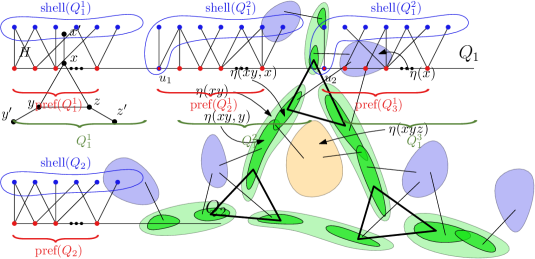
Figure 2: Definitions of $\mathrm{pref}(\mathcal{S})$ and $\mathrm{shell}(\mathcal{S})$ in case of $|Q_{2}|\geq t$.

Now, we use the algorithm from Theorem 2.2 on $Z$ being the set of the first vertices of paths in $\mathcal{S}_{\geq t}$ and the graph defined as $G-\mathrm{shell}(\mathcal{S})$. If Theorem 2.2 produced an induced tree with three leaves among $Z$, we return it as an induced $S_{t,t,t}$, since those must have been induced branches at least $t$ vertices long in $G-\mathrm{shell}(\mathcal{S})$. Hence, we obtained an extended strip decomposition $(H^{\prime},\eta^{\prime})$ of $G-\mathrm{shell}(\mathcal{S})$. If the obtained decomposition is refined, we return $\mathcal{P}\coloneqq\mathrm{pref}(\mathcal{S})$, $X\coloneqq\mathrm{shell}(\mathcal{S})$, and the extended strip decomposition $(H\coloneqq H^{\prime},\eta\coloneqq\eta^{\prime})$.

Therefore, the obtained extended strip decomposition $(H^{\prime},\eta^{\prime})$ of $G-\mathrm{shell}(\mathcal{S})$ contains a particle $A$ which is not small, i.e., $A$ is composed of at least $\frac{n}{2}$ vertices. As $Z$ is peripheral, we know that no three paths in $\mathcal{S}_{\geq t}$ touch one particle by Theorem 2.4. Therefore, we take the set $\hat{\mathcal{Q}}$ of at most two paths, say $P_{1}$ and $P_{2}$, touching $A$ (for convenience, let $P_{1}$ or $P_{2}$ be an empty set if it does not exist). We now compute the maximum proportion of $\bigcup\mathcal{Q}$ put to $\hat{\mathcal{Q}}$. If both $P_{1},P_{2}\subseteq Q_{1}$, then this fraction is at most $\frac{2}{3}$ as by the definition $|Q_{1}^{i}|\leq\frac{|Q_{1}|}{3}$, for $i\in\{1,2,3\}$. If one is $Q_{2}$ and the other comes from $Q_{1}$, then we estimate $a+\frac{1-a}{3}=\frac{2a+1}{3}\leq\frac{2}{3}$ for $a={|Q_{2}|}/{|\bigcup\mathcal{Q}|}\leq\frac{1}{2}$. Hence, we know that $|\bigcup\hat{\mathcal{Q}}|\leq\frac{2}{3}|\bigcup\mathcal{Q}|$. We define $\hat{G}\coloneqq A\cup P_{1}\cup P_{2}$ to use Lemma 3.1 on a smaller instance. Now, we need to verify that the assumption of the lemma holds. We claim the following:

Claim 1.

$\hat{G}-N[\bigcup{\hat{\mathcal{Q}}}]$ has a refined extended strip decomposition.

As $\hat{G}$ is an induced subgraph of $G$ and $G-N[\bigcup{\mathcal{Q}}]$ has a refined extended strip decomposition, we know that $\hat{G}-N[\bigcup{\mathcal{Q}}]$ has a refined extended strip decomposition. First, recall that $N[u_{1}]-(Q_{1}^{1}\cup Q_{1}^{2})\subseteq\mathrm{shell}(Q_{1}^{2})$, which is disjoint with $V(\hat{G})$. Analogously $N[u_{2}]-(Q_{1}^{2}\cup Q_{1}^{3})$ is disjoint with $V(\hat{G})$. Also, if $|Q_{2}|<t$ then $Q_{2}$ is disjoint with $V(\hat{G})$ as well. Hence, $\hat{G}-N[\bigcup{\mathcal{Q}}]\simeq\hat{G}-N[\bigcup{\mathcal{S}_{\geq t}}]$. Also, recall that the only paths among $\mathcal{S}_{\geq t}$ that touch $A$ are in $\hat{\mathcal{Q}}$. Hence, observe that $\hat{G}-N[\bigcup{\mathcal{S}_{\geq t}}]\simeq\hat{G}-N[\bigcup{\hat{\mathcal{Q}}}]$.

Therefore, we can apply Lemma 3.1 inductively on $\hat{G}$ and $\hat{\mathcal{Q}}$, obtaining $\hat{\mathcal{P}}$ and $\hat{X}$, and a refined extended strip decomposition $(\hat{H},\hat{\eta})$ of $\hat{G}-\hat{X}$. We need to combine the extended strip decomposition obtained from the recursion with the extended strip decomposition $(H^{\prime},\eta^{\prime})$ we obtained earlier.

We can always suppose that particle $A$ is of type $A^{xy}_{xy}$ for some edge $xy\in E(H^{\prime})$, unless $A$ is of type $A_{x}$ for an isolated vertex $x\in V(H^{\prime})$. That is because $A^{xy}_{xy}$ is the superset of all possible particle types. As Theorem 2.2 gives us that both $\eta^{\prime}(xy,x)$ and $\eta^{\prime}(xy,y)$ are nonempty, we can select $v_{x}\in\eta^{\prime}(xy,x)$ and $v_{y}\in\eta^{\prime}(xy,y)$ (possibly $v_{x}=v_{y}$). By Section 2, the set

$$X^{\prime}\coloneqq\left(N(v_{y})\cup N(v_{x})\right)-V(A)$$

separates $A$ from the rest of $G$. Set $\mathcal{P}^{\prime}\coloneqq\left\{\{v_{x}\},\{v_{y}\}\right\}$. In the case of $A_{x}$ such that $x\in V(H)$ is an independent vertex, we set $\mathcal{P}^{\prime}\coloneqq\emptyset$ and $X^{\prime}\coloneqq\emptyset$ and still such $A$ is separated from the rest of $G$ by $X^{\prime}$. We return:

• $\mathcal{P}\coloneqq\hat{\mathcal{P}}\cup\mathcal{P}^{\prime}\cup\mathrm{pref}(\mathcal{S})$,

• $X\coloneqq\hat{X}\cup X^{\prime}\cup\mathrm{shell}(\mathcal{S})$,

• an extended strip decomposition $(H,\eta)$ of $G-X$, where $H$ is $\hat{H}$ with an additional isolated vertex $w$, and $\eta$ is $\hat{\eta}$ with an additional trivial vertex particle $\eta(w)$ containing all vertices of $G-X-A$.

We compute that $|\mathcal{P}|\leq 6+6\log_{3/2}\left(\left|\bigcup{\hat{\mathcal{Q}}}\right|\right)+6\leq 6\log_{3/2}\left(\left|\bigcup{\mathcal{Q}}\right|\right)+6$ as we added at most six new paths into $\mathcal{P}$. Observe that the described algorithm runs in polynomial time as we just computed that the depth of recurrence is logarithmic in $|\bigcup(\mathcal{Q})|\leq|V(G)|$ and each recursive call takes polynomial time in the size of $G$.

Proof 3.3 (Proof of Theorem 1.2).

Using Theorem 1.1 we find a Gyárfás path $Q$. We get the desired outcome by Lemma 3.1 on $G$ with $\mathcal{Q}\coloneqq\{Q\}$. The extended strip decomposition needed by the lemma’s assumption is trivial. That is, each connected component of $G-Q$ is represented by a vertex particle of small size. We conclude the proof of Theorem 1.2 by the following calculation:

$$6\log_{3/2}n+6\leq 11\log n+6.$$

Note that for any extended strip decomposition $(H,\eta)$ we can easily add the assumption that sets $\eta(xy,x)\neq\emptyset$ for any edge $xy\in E(H)$. As suppose $\eta(xy,x)=\emptyset$; then we can update $(H,\eta)$ by adding $\eta(xy)$ to $\eta(y)$ and removing $xy$ from $H$. Moreover, we can simply remove any empty trivial vertex particle form $\eta$ and the corresponding isolated vertex from $H$. Therefore, we may suppose that the obtained extended strip decomposition is rigid.

In the following simple corollary we apply Theorem 1.2 to $sS_{t,t,t}$-free graphs, for some $s,t\geq 1$.

Corollary 3.4.

Let $s\geqslant 1,t\geqslant 1$ be constants. Let $G$ be an $sS_{t,t,t}$-free graph on $n$ vertices. Then in polynomial time we can find a set $X$ consisting of at most $(s-1)(3t+1)+(11\log n+6)(t+1)$ vertices and a rigid extended strip decomposition of $G-N[X]$ whose every particle has at most $n/2$ vertices.

Proof 3.5.

Induction on $s$. If $s=1$, then we obtain the result immediately by Theorem 1.2. Thus let us assume that $s\geqslant 2$ and the theorem holds for $(s-1)S_{t,t,t}$-free graphs.

We exhaustively check if there is some $Y\subseteq V(G)$ with $|Y|=3t+1$, such that $G[Y]\simeq S_{t,t,t}$; we can do it in time $n^{3(t+1)+\mathcal{O}(1)}=n^{\mathcal{O}(1)}$. If such $Y$ does not exist, then we can immediately apply Theorem 1.2, and the proof is complete. Thus suppose that $Y$ exists.

We observe that the graph $G^{\prime}:=G-N[Y]$ is $(s-1)S_{t,t,t}$-free. Denote $n^{\prime}:=|V(G^{\prime})|$. By the inductive assumption, in time $(n^{\prime})^{\mathcal{O}(1)}=n^{\mathcal{O}(1)}$ we can obtain a set $X^{\prime}\subseteq V(G^{\prime})$ of size at most $(s-2)(3t+1)+(11\log n^{\prime}+6)(t+1)$ and a rigid extended strip decomposition $(H,\eta)$ of $G^{\prime}-N[X^{\prime}]$ whose every particle is of size at most $n^{\prime}/2$.

We set $X=Y\cup X^{\prime}$. Now $X$ and $(H,\eta)$ satisfy the statement of the theorem, as $G^{\prime}-N[X^{\prime}]=G-N[X]$ and $n^{\prime}\leqslant n$. The total running time is polynomial in $n$ as the depth of the recursion is $s-1$.

4 Algorithmic applications

In this section we will show how to combine Theorem 1.2 with the approach of Chudnovsky et al. [10, 11] in order to obtain a QPTAS and a subexponential-time algorithm for MWIS in $S_{t,t,t}$-free graphs, i.e., we prove Theorems 1.3 and 1.4.

Both algorithms follow the same general outline; let us sketch it before we get into the details of each particular case. Each algorithm is a recursive procedure, which consists of two phases. In the first one, we deal with the vertices of $G$ that are heavy, which means that their neighborhood is “large”, where the exact meaning of “large” depends on the particular algorithm.

Once there are no heavy vertices, i.e., the neighborhood of each vertex is “small”, we proceed to the second phase. We call Corollary 3.4 for the current instance $G$, obtaining a small-sized set $X$ and a rigid extended strip decomposition $(H,\eta)$ of $G-N[X]$, whose every particle is of small size. The crux is that since we are in the second phase, all vertices in $X$ are not heavy, and since $X$ is of small size, the whole set $N[X]$ is “small”. We treat $N[X]$ separately in a way that depends on the particular algorithm.

Next, for each particle $A$ of $(H,\eta)$, we call the algorithm recursively for $G[A]$, obtaining (a good approximation of) a maximum-weight independent set in $G[A]$. Finally, we combine the obtained results to derive (a good approximation of) a maximum-weight independent set in $G$. This last step is based on the idea of Chudnovsky et al. [10, 11] to reduce the problem to finding a maximum-weight matching in a graph obtained by a simple modification of $H$. Since the size of $H$ is linear in $|V(G)|$ (by Figure 1), this problem can be solved in time polynomial in $|V(G)|$ using, e.g., the classic algorithm of Edmonds [14]. The last step is encapsulated in the following lemma, whose exact statement comes from Abrishami et al. [1].

Lemma 4.1 (Chudnovsky et al. [10, 11]).

Let $\varsigma\in[0,1]$ be a real number. Let $G$ be an $n$-vertex graph equipped with a weight function $\mathfrak{w}:V(G)\to\mathbb{Z}_{\geqslant 0}$. Suppose that $G$ is given along with an extended strip decomposition $(H,\eta)$, where $H$ has $N$ vertices.

Let $I_{0}\subseteq V(G)$ be a fixed independent set in $G$. Furthermore, assume that for each particle $A$ of $(H,\eta)$ we are given an independent set $I(A)$ in $G[A]$ such that $\mathfrak{w}(I(A))\geqslant\varsigma\cdot\mathfrak{w}(I_{0}\cap A)$. Then in time polynomial in $n+N$ we can compute an independent set $I$ in $G$ such that $\mathfrak{w}(I)\geqslant\varsigma\cdot\mathfrak{w}(I_{0})$.

Let us stress out that the algorithm from Lemma 4.1 does not need to know the value of $\varsigma$ or the independent set $I_{0}$.

The main difference between our approach and the one of Chudnovsky et al. [11] is that we use Theorem 1.2 and its consequence, i.e., Corollary 3.4. The previous algorithms used a similar statement but with a worse (and much more involved) guarantee on the size of $X$ and each particle. Furthermore, the way we obtain our set $X$ is significantly simpler.

4.1 Proof of Theorem 1.3

Before we proceed to the proof, let us first explain the meaning of “small”, and how to deal with $N[X]$ in this particular case. Here the neighborhood of a vertex is “small” if it has few vertices (more specifically, at most $\sqrt{n/t}$). In the first phase, we deal with heavy vertices $v$ (i.e., of large degree) with simple branching: we guess whether $v$ is included in our optimum solution or not. Since the degree of $v$ is large, in the first branch, we obtain significant progress, which is enough to obtain a subexponential running time.

In the second phase, since $N[X]$ is the neighborhood of $\mathcal{O}(\log n)$ vertices, each of degree $\mathcal{O}(\sqrt{n})$, the total size of $N[X]$ is $\mathcal{O}(\sqrt{n}\log n)$. Thus we can afford to exhaustively guess the intersection of our optimum solution with $N[X]$.

Proof 4.2 (Proof of Theorem 1.3).

Let $s,t\geqslant 1$ be constants and let $(G,\mathfrak{w})$ be an instance of MWIS, where $G$ is $sS_{t,t,t}$-free and has $n$ vertices. We observe that if $n$ is small, i.e., bounded by a constant. Then we can solve the problem by brute force. Thus we assume that $n\geqslant n_{0}$, where $n_{0}$ is a constant (depending on $s$ and $t$) whose exact value follows from the reasoning below.

First, consider the case that there exists $v\in V(G)$ such that $\deg v\geqslant\sqrt{n/t}$. We branch on including $v$ in the final solution: we either delete $v$ from $G$, or we delete $N[v]$ and add $v$ to the solution returned by the recursive call. Then we output the one of these two solutions that has a larger weight. The correctness of this step of the algorithm is straightforward.

Hence, we can assume that for every $v\in V(G)$ it holds that $\deg v\leqslant\sqrt{n/t}$. By Corollary 3.4, since $G$ is $sS_{t,t,t}$-free, we obtain a set $X$ of size $(s-1)(3t+1)+(11\log{n}+6)(t+1)\leqslant 12(t+1)\log n$ (here we use that $n$ is large), and a rigid extended strip decomposition $(H,\eta)$ of $G^{\prime}=G-N[X]$ whose every particle has at most $n/2$ vertices.

We exhaustively guess an independent set $J\subseteq N[X]$; think of it as an intersection of the intended optimum solution with $N[X]$. Consider the graph $G^{\prime\prime}:=G^{\prime}-N[J]$. We modify $(H,\eta)$ by removing the vertices from $N[J]$ from the sets $\eta(\cdot)$. Let us call the obtained strip decomposition $(H,\eta^{\prime})$; note that it might not be rigid. We call the algorithm recursively for the subgraph $G^{\prime\prime}[A]$ for every nonempty particle $A$ of $(H,\eta^{\prime})$. Let $I(A)$ be the solution. If $A=\emptyset$, then $I(A)=\emptyset$. By the inductive assumption $I(A)$ is a maximum-weight independent set in $G^{\prime\prime}[A]$. Then we use Lemma 4.1 for $\varsigma=1$ to combine the solutions into a maximum-weight independent set $I_{J}$ of $G^{\prime\prime}$. Finally, we return the independent set $J\cup I_{J}$ whose weight is maximum over all choices of $J$. Note that the correctness of this step is guaranteed by the exhaustive guessing of $J$ and Lemma 4.1.

Running time.

Let $F(n)$ denote the running time of our algorithm for $n$-vertex instances. We prove that $F(n)=2^{\mathcal{O}\left(\sqrt{tn}\log{n}\right)}$. If $n<n_{0}$, then the claim clearly holds. So let us assume that $n\geqslant n_{0}$.

In the first case we call the algorithm for two instances, one of size $n-1$ and one of size at most $n-\sqrt{n/t}$. Hence,

$$F(n)\leqslant F(n-1)+F(n-\sqrt{n/t})=2^{\mathcal{O}\left(\frac{n\log{n}}{\sqrt{n/t}}\right)}\leqslant 2^{\mathcal{O}\left(\sqrt{tn}\log{n}\right)}.$$

Here we skip the description how this recursion is solved, as it it pretty standard. For a formal proof we refer the reader to Bacsó et al. [7, Lemma 1].

It remains to analyze the running time of the step in which the maximum degree of vertices in $G$ is bounded by $\sqrt{n/t}$. Corollary 3.4 asserts that we obtain $X$ and the rigid extended strip decomposition $(H,\eta)$ of $G^{\prime}=G-N[X]$ in time polynomial in $n$. There are $2^{\mathcal{O}(\sqrt{n/t}\cdot t\log{n})}=2^{\mathcal{O}(\sqrt{nt}\log{n})}$ ways of choosing the set $J$. In polynomial time we modify $(H,\eta)$ into $(H,\eta^{\prime})$.

Observe that while $(H,\eta^{\prime})$ might not be rigid, it was obtained from a rigid extended strip decomposition $(H,\eta)$ by deleting some vertices from the sets $\eta(\cdot)$. In particular, both decompositions have the same sets of particles, and every nonempty particle of $(H,\eta^{\prime})$ is also a nonempty particle of $(H,\eta)$. Thus by Section 2 we call the algorithm recursively for at most $4n$ nonempty particles, each of size at most $n/2$. By Figure 1, the total number of particles of $(H,\eta^{\prime})$ is polynomial in $n$. Finally, having computed a maximum independent set contained in each particle, by Lemma 4.1, we can compute the final solution in time polynomial in $n$. Hence, there are constants $c,c_{1},c_{2}$, where $c\gg c_{1},c_{2}$, such that total running time of this step is bounded by:

$$F(n)\leqslant 2^{c_{1}\cdot\sqrt{nt}\log{n}}\left(n^{c_{2}}+4n\cdot 2^{c\cdot\sqrt{tn/2}\log{(n/2)}}\right)\overset{c\gg c_{1},c_{2}}{\leqslant}2^{c\cdot\sqrt{tn}\log{n}},$$ (1)

and so is the total complexity of the algorithm.

4.2 Proof of Theorem 1.4

Again let us start with explaining the algorithm-specific details of the outline presented at the start of Section 4.

We will use the notion of $\beta$-heavy vertices from [10, 11]. Consider a graph $G$, a weight function $\mathfrak{w}:V(G)\to\mathbb{Z}_{\geqslant 0}$, and an independent set $I\subseteq V(G)$. Let $\beta\in(0,1/2]$ be a real. We say that a vertex $v\in V(G)$ is $\beta$-heavy (with respect to $I$) if $\mathfrak{w}(N[v]\cap I)>\beta\cdot\mathfrak{w}(I)$. A set $J$ is good for $I$ if $J\subseteq I$ and $N[J]$ contains all vertices that are $\beta$-heavy with respect to $I$.

Lemma 4.3 (Chudnovsky et al. [10, 11]).

Let $G$ be an $n$-vertex graph for $n>2$, $\mathfrak{w}:V(G)\to\mathbb{Z}_{\geqslant 0}$ be a weight function, $I\subseteq V(G)$ be an independent set, and $\beta\in(0,1/2]$ be a real. Then there exists a set $J$ of size at most $\lceil\beta^{-1}\log{n}\rceil$ which is good for $I$.

Now the vertex is heavy if it is $\beta$-heavy for some carefully chosen parameter $\beta$. This means that a neighborhood of a vertex is “large” if it contains a significant ($\geqslant\beta$) fraction of the weight of $I_{\mathsf{OPT}}$. In the first phase, we exhaustively guess the set $J$ that is good for a fixed optimum solution $I_{\mathsf{OPT}}$. Note that $J$ is of small size and since $J\subseteq I_{\mathsf{OPT}}$, we know that $N(J)$ contains no vertices from $I_{\mathsf{OPT}}$ and thus can be safely removed from the graph.

Since $J$ is good for $I_{\mathsf{OPT}}$, we know that $G-N[J]$ contains no heavy vertices, and for this graph we call Corollary 3.4. Now, as $N[X]$ is a neighborhood of few non-heavy vertices, we know that the total weight of $I_{\mathsf{OPT}}\cap N[X]$ is small and thus can be sacrificed, as we aim for an approximation.

Proof 4.4 (Proof of Theorem 1.4).

Let $s,t\geqslant 1$ be constants and let $(G,\mathfrak{w})$ be an instance of MWIS, where $G$ is $sS_{t,t,t}$-free and has $n$ vertices. Let $\varepsilon\in(0,1)$ be fixed. Fix a maximum-weight independent set $I_{\mathsf{OPT}}$ in $G$ with respect to $\mathfrak{w}$. We describe a procedure that finds in $G$ an independent set $I$ of weight at least $(1-\varepsilon)\cdot\mathfrak{w}(I_{\mathsf{OPT}})$.

Let $N$ be the minimum power of two greater than or equal to the size of our initial instance. Note that $n\leqslant N<2n$. The value of $N$ will not change throughout the execution of the algorithm.

The algorithm itself is a recursive procedure. The arguments of each call are a graph $G^{\prime}$, which is an induced subgraph of $G$, the weight function on $V(G^{\prime})$ obtained by restricting the domain of $\mathfrak{w}$, and an integer $h$, which can be intuitively understood as the depth of the current call in the recursion tree. Since it does not lead to confusion, we will always denote the weight function by $\mathfrak{w}$. We will keep the invariant that for each call $(G^{\prime},\mathfrak{w},h)$ it holds that $|V(G^{\prime})|\leqslant N/2^{h}$. The initial call, corresponding to the root of the recursion tree, is for $(G,\mathfrak{w},0)$.

Consider a call for the instance $(G^{\prime},\mathfrak{w},h)$. If $|V(G^{\prime})|<n_{0}$, where $n_{0}$ is a constant (depending on $s$ and $t$) that follows from the reasoning below, then we can solve the problem by brute force. Thus let us assume that $n\geqslant n_{0}$. In particular, $N>1$.

We set

$$\beta(h,\varepsilon):=\frac{\varepsilon}{12(t+1)\log{(N/2^{h})}\cdot\left((1-\varepsilon)\log{N}+\varepsilon(h+1)\right)}.$$ (2)

It is straightforward to verify that for $h<\log N$ we have $\beta(h,\varepsilon)\in(0,1/2]$. On the other hand, if $h\geqslant\log N$, then $G^{\prime}$ is of constant size and thus $\beta(h,\varepsilon)$ is not computed for such $h$.

Let $\mathcal{J}$ be the family of all independent sets in $G^{\prime}$ of size at most $\lceil\beta(h,\varepsilon)^{-1}\log{(N/2^{h})}\rceil$. For each $J\in\mathcal{J}$ we proceed as follows. If $|V(G^{\prime}-N[J])|<n_{0}$, then we compute a maximum-weight independent set $I_{J}$ in $G^{\prime}-N[J]$ by brute force. Otherwise, we use Corollary 3.4, to obtain a set $X_{J}\subseteq V(G^{\prime}-N[J])$ and a rigid extended strip decomposition $(H,\eta)$ of $G^{\prime}-N[J]-N[X_{J}]$ such that each particle of $(H,\eta)$ is of size at most $|V(G^{\prime}-N[J])|/2$. By Corollary 3.4, we obtain

$$\begin{split}|X_{J}|\leqslant\ &(s-1)(3t+1)+(11\log|V(G^{\prime}-N[J])|+6)(t+1)\\ \leqslant\ &12(t+1)\log|V(G^{\prime})|\leqslant 12(t+1)\log(N/2^{h}).\end{split}$$ (3)

Let $Y_{J}:=N(J)\cup N[X_{J}]$. We modify $(H,\eta)$ into an extended strip decomposition of $G^{\prime}-Y_{J}$ as follows. For each $v\in J$, we add to $H$ an isolated vertex $x_{v}$, and set $\eta(x_{v})=\{v\}$. Let us call this extended strip decomposition $(H^{\prime},\eta^{\prime})$. Observe that each particle of $(H^{\prime},\eta^{\prime})$ is of size at most $|V(G^{\prime}-N[J])|/2\leqslant|V(G^{\prime})|/2$. Furthermore, since $(H,\eta)$ is rigid, so is $(H^{\prime},\eta^{\prime})$.

For each nonempty particle $A$ of $(H^{\prime},\eta^{\prime})$ we call the algorithm recursively on an instance $(G^{\prime}[A],\mathfrak{w},h+1)$. Let $I(A)$ be the value returned by the algorithm. For each empty particle $A$ we set $I(A):=\emptyset$. Finally, we apply the algorithm from Lemma 4.1, in order to obtain an independent set $I_{J}$ of $G^{\prime}-Y_{J}$ and thus of $G^{\prime}$. Recall that the value of $\varsigma$ is not needed to apply Lemma 4.1; we will define it in the next paragraph when we discuss the approximation guarantee. As the solution, we return the set $I_{J}$ of maximum weight, over all choices of $J\in\mathcal{J}$.

Approximation guarantee.

Consider the recursion tree of our algorithm. We mark some nodes of the recursion tree. First, we mark the root. Now consider some marked node $z$ corresponding to a call $(G^{\prime},\mathfrak{w},h)$, such that $z$ is not a leaf node. Observe that by Lemma 4.3, there is some $J\in\mathcal{J}$ (for this particular instance) which is good for $I_{\mathsf{OPT}}\cap V(G^{\prime})$. Fix such $J$. If there is more than one, we choose one arbitrarily. We mark the children of $z$ that correspond to the calls on the particles of the extended strip decomposition of $G^{\prime}-Y_{J}$.

Let $\mathcal{T}$ be the subtree of the recursion tree induced by the marked nodes. Note that each leaf of $\mathcal{T}$ is a leaf of the whole recursion tree, i.e., it corresponds to an instance of constant size. Since at each level of the recursion, the size of the instance drops by at least half, we observe that each instance at level $h$ (where the root is at level 0) is of size at most $N/2^{h}$. Consequently, the depth of $\mathcal{T}$ is at most $\log N$.

Consider a call for an instance $(G^{\prime},\mathfrak{w},h)$ and let $J$ be good for $I_{\mathsf{OPT}}$. Let us estimate $\mathfrak{w}(I_{\mathsf{OPT}}\cap Y_{J})$. First, observe that since $J\subseteq I_{\mathsf{OPT}}$, we have that $\mathfrak{w}(I_{\textsf{OPT}}\cap N(J))=0$. Moreover, since $J$ was chosen to be good, there are no $\beta(h,\varepsilon)$-heavy vertices in $V(G^{\prime}-N[J])$, and in particular, in $N[X_{J}]$. Hence,

$$\begin{split}\mathfrak{w}(I_{\textsf{OPT}}\cap Y_{J})=\ &\mathfrak{w}(I_{\textsf{OPT}}\cap N[X_{J}])\leqslant|X_{J}|\cdot\beta(h,\varepsilon)\cdot\mathfrak{w}(I_{\textsf{OPT}}\cap V(G^{\prime}))\\ \overset{\eqref{eq:qptas-beta}\text{ and }\eqref{eq:sizex}}{\leqslant}\ &\frac{\varepsilon}{(1-\varepsilon)\log N+\varepsilon(h+1)}\cdot\mathfrak{w}(I_{\textsf{OPT}}\cap V(G^{\prime})).\end{split}$$ (4)

The following claim shows that the solution computed for the instance $(G^{\prime},\mathfrak{w},h)$ at each node of $\mathcal{T}$ is a reasonable approximation of $I_{\mathsf{OPT}}\cap V(G^{\prime})$.

Claim 2.

Let $z$ be a node of $\mathcal{T}$, and let $(G^{\prime},\mathfrak{w},h)$ be the instance corresponding to $z$. Let $I$ be the independent set returned by the algorithm for the call at $z$. Then $\mathfrak{w}(I)\geqslant\left(1-\varepsilon+\frac{\varepsilon h}{\log{N}}\right)\cdot\mathfrak{w}\left(I_{\mathsf{OPT}}\cap V(G^{\prime})\right)$.

First, observe that if $z$ is a leaf of $\mathcal{T}$, then the statement of the claim is satisfied. Indeed, in this case $I$ is computed by brute force, and hence $\mathfrak{w}(I)=\mathfrak{w}(I_{\mathsf{OPT}}\cap V(G^{\prime}))$.

Recall that the algorithm returns the solution of maximum weight among all choices of $J\in\mathcal{J}$, so clearly we have $\mathfrak{w}(I)\geqslant\mathfrak{w}(I_{J})$, where $J$ is good for $I_{\mathsf{OPT}}\cap V(G^{\prime})$.

We proceed by induction on $h$. First, consider a node $z$ at the level $h=\log{N}$. As the depth of $\mathcal{T}$ is at most $\log N$, we observe that $z$ must be a leaf, so the claim follows by the observation above.

Assume that the claim holds for $h+1\in[\log{N}]$ and consider a node $z$ at level $h$. If $z$ is a leaf, then again, we are done. Otherwise, let $\mathcal{A}$ be the set of nonempty particles of the extended strip decomposition of $G^{\prime}-Y_{J}$. For every such particle $A$, we recursively computed an independent set $I(A)$. By the inductive assumption, we have that $\mathfrak{w}(I(A))\geqslant\left(1-\varepsilon+\frac{\varepsilon(h+1)}{\log{N}}\right)\mathfrak{w}(I_{\textsf{OPT}}\cap V(G^{\prime}[A]))$; note that these recursive calls are at level $h+1$. Clearly, the same holds for empty particles because $\emptyset$ is there an optimum solution.

Thus, by Lemma 4.1 applied to $I_{\mathsf{OPT}}$ and $\varsigma=1-\varepsilon+\frac{\varepsilon(h+1)}{\log{N}}$, we obtain an independent set $I_{J}$ in $G^{\prime}-Y_{J}$, such that

$$\begin{split}\mathfrak{w}(I_{J})\geqslant\ &\left(1-\varepsilon+\frac{\varepsilon(h+1)}{\log{N}}\right)\mathfrak{w}(I_{\textsf{OPT}}\cap V(G^{\prime}-Y_{J}))\\ =\ &\left(1-\varepsilon+\frac{\varepsilon(h+1)}{\log{N}}\right)\biggl{(}\mathfrak{w}(I_{\textsf{OPT}}\cap V(G^{\prime}))-\mathfrak{w}(I_{\textsf{OPT}}\cap Y_{J})\biggr{)}.\end{split}$$ (5)

Combining (5) with (4) and simplifying the formula, we obtain

$$\mathfrak{w}(I_{J})\geqslant\left(1-\varepsilon+\frac{\varepsilon h}{\log{N}}\right)\mathfrak{w}(I_{\textsf{OPT}}\cap V(G^{\prime})),$$

which concludes the proof of the claim.

Since the root of the recursion tree belongs to $\mathcal{T}$, the final result $I$ returned for the call at the root (i.e., for $(G,\mathfrak{w},0)$) satisfies

$$\mathfrak{w}(I)\geqslant\left(1-\varepsilon\right)\cdot\mathfrak{w}\left(I_{\mathsf{OPT}}\cap V(G)\right)=(1-\varepsilon)\cdot\mathfrak{w}(I_{\mathsf{OPT}}).$$

This concludes the discussion of the approximation guarantee.

Running time.

Recall that the recursion tree has depth at most $\log N$. Let us show the following claim concerning the running time.

Claim 3.

Let $z$ be a node of the recursion tree, and let $(G^{\prime},\mathfrak{w},h)$ be the instance corresponding to $z$. Then the algorithm solves this instance in time $2^{\mathcal{O}\left(\varepsilon^{-1}\log^{4}N\log\left(N/2^{h-1}\right)\right)}$.

Let $F(h)$ denote the upper bound for the running time of our algorithm, depending on the level of the call in the recursion tree. We aim to show that there is an absolute constant $c$, such that for $N$ sufficiently large we have

$$F(h)\leqslant 2^{c\cdot\varepsilon^{-1}\log^{4}N\log\left(N/2^{h-1}\right)}.$$

Recall that $|V(G^{\prime})|\leqslant N/2^{h}$. If $z$ is a leaf, then the instance is of constant size, and thus the claim holds (assuming that $c$ is sufficiently large). In particular this happens if $h=\log N$. So let us assume that the claim holds for the calls at level $h+1$ and that $h<\log N$.

Recall that we first enumerate the family $\mathcal{J}$ of all independent sets of size at most $\lceil\beta(h,\varepsilon)^{-1}\log(N/2^{h})\rceil$. Observe that

$$|\mathcal{J}|\leqslant\ |V(G^{\prime})|^{\lceil\beta(h,\varepsilon)^{-1}\log(N/2^{h})\rceil}\leqslant 2^{\log(N/2^{h})\lceil\beta(h,\varepsilon)^{-1}\log(N/2^{h})\rceil},$$

and the family $\mathcal{J}$ can be enumerated in time polynomial in its size.

For each $J\in\mathcal{J}$, using Corollary 3.4 and modifying its outcome, in polynomial time we obtain a set $X_{J}$ and a rigid extended strip decomposition $(H^{\prime},\eta^{\prime})$ of $G-Y_{J}$, where $Y_{J}=N[X_{J}]\cup N(J)$.

Next, we call the algorithm recursively for at most $4\cdot|V(G^{\prime})|\leqslant 4\cdot N/2^{h}$ instances, each at depth $h+1$. Finally, use use Lemma 4.1 to obtain our solution in time polynomial in $|V(G^{\prime})|$ and thus in $N/2^{h}$.

Thus the running time is bounded by the following expression (here $c_{1},c_{2},c_{3}$ are absolute constants, such that $c_{1}$ and $c_{2}$ are much smaller than $c_{3}$, and $c_{3}=c/12(t+1)$):

$$F(h)\leqslant\ 2^{c_{1}\cdot\beta(h,\varepsilon)^{-1}\log^{2}(N/2^{h})}\cdot\left((N/2^{h})^{c_{2}}+4\cdot(N/2^{h})\cdot F(h+1)\right)$$

$$\overset{c_{3}\gg c_{1},c_{2}}{\leqslant}\ 2^{c_{3}\cdot\beta(h,\varepsilon)^{-1}\log^{2}(N/2^{h})}\cdot 2^{c\cdot\varepsilon^{-1}\log^{4}N\log(N/2^{h})}$$

$$=\ \exp\ \Bigl{\{}c_{3}\cdot\beta(h,\varepsilon)^{-1}\log^{2}(N/2^{h})+c\cdot\varepsilon^{-1}\log^{4}N\log(N/2^{h})\Bigr{\}}$$

$$\leqslant\ \exp\ \Bigl{\{}c_{3}\cdot 12(t+1)\cdot\left(\frac{1-\varepsilon}{\varepsilon}\log N+(h+1)\right)\log^{3}(N/2^{h})+c\cdot\varepsilon^{-1}\log^{4}N\log(N/2^{h})\Bigr{\}}$$

$$\overset{h<\log N}{\leqslant}\ \exp\ \Bigl{\{}c\cdot\varepsilon^{-1}\log^{4}N+c\cdot\varepsilon^{-1}\log^{4}N\log(N/2^{h})\Bigr{\}}$$

$$=\ \exp\ \Bigl{\{}c\cdot\varepsilon^{-1}\log^{4}N(\log(N/2^{h})+1)\Bigr{\}}=\exp\ \Bigl{\{}c\cdot\varepsilon^{-1}\log^{4}N\log(N/2^{h-1})\Bigr{\}}.$$

This completes the proof of the claim. Now we apply 3 to the initial call $(G,\mathfrak{w},0)$ and obtain that the overall running time is

$$2^{\mathcal{O}(\varepsilon^{-1}\log^{5}N)}=2^{\mathcal{O}(\varepsilon^{-1}\log^{5}n)},$$

as $N<2n$. This completes the proof.

5 Conclusion

In the QPTAS of Chudnovsky, Pilipczuk, Pilipczuk, and Thomassé [10, 11] it was more convenient to measure the weight of parts of the graph not by the number of vertices, but by the weight of the intersection of the sought solution with the part in question. We observe that we can adapt Theorem 1.2 to this setting of unknown weight function.

Theorem 5.1.

Given an $n$-vertex graph $G$ and an integer $t$, one can in time $n^{\mathcal{O}(t\log n)}$ either:

• output an induced copy of $S_{t,t,t}$ in $G$, or

• output a family $\mathcal{F}$ satisfying the following:

  1. every element of $\mathcal{F}$ is a pair of a set $\mathcal{P}$ consisting of at most $11\log n+6$ induced paths in $G$, each of length at most $t+1$, and an extended strip decomposition of $G-N[\bigcup{\mathcal{P}}]$;

  2. for every weight function $\mathfrak{w}:V(G)\to\mathbb{Z}_{\geqslant 0}$ there exists a pair in $\mathcal{F}$ such that every particle in the extended strip decomposition of the pair has weight at most half of the total weight of $G$;

  3. the size of $\mathcal{F}$ is bounded by $n^{\mathcal{O}(\log n)}$.

Proof 5.2 (Proof sketch.).

As observed in [10, 11], in $G$ one can identify at most $n^{2}$ induced paths such that for every weight function $\mathfrak{w}:V(G)\to\mathbb{Z}_{\geqslant 0}$, at least one of the identified path is a Gyárfás’ path for $\mathfrak{w}$, that is, a path $Q$ such that every connected component of $G-N[Q]$ is of weight at most half of the weight of $G$. Thus, we can guess the path $Q$ as in the proof in Theorem 1.2 out of at most $n^{2}$ candidates.

Then, in the recursive step in the proof of Theorem 1.2, instead of choosing the heavy particle to recurse on, we guess which particle is heavy (or that none exists). It is easy to see that any extended strip decomposition in the process will have fewer than $n$ inclusion-wise maximal particles; thus, this gives $n^{\mathcal{O}(\log n)}$ possible outputs to enumerate.

We think the $\log n$ factor in Theorem 1.2 is an artifact of our technique, and is not necessary. Therefore, we pose the following conjecture.

Conjecture 5.3.

For every integer $t\geqslant 1$ there exists a constant $\varepsilon>0$ and an integer $s$ such that every $S_{t,t,t}$-free graph $G$ admits a set $P\subseteq V(G)$ of size at most $s$ such that $G-N[P]$ admits a rigid extended strip decomposition whose every particle has at most $(1-\varepsilon)|V(G)|$ vertices.

Abrishami, Chudnovsky, Dibek, and Rzążewski [2] very recently announced a polynomial-time algorithm for MWIS in $S_{t,t,t}$-free graphs of bounded degree. Their argument is quite involved and revisits the proof of the three-in-a-tree theorem [13].

Confirming Conjecture 5.3 would imply the same result almost immediately, possibly with a better running time. Indeed, one needs to branch on $N[P]$ and recurse on the remainder of every particle of $(H,\eta)$. The maximum degree of $H$ is bounded by a function of the maximum degree of $G$ (i.e., is a constant), which ensures that the sum of sizes of all particles is linear in $|V(G)|$. This in turns implies that the total complexity of the algorithm can be bounded by a polynomial function. Note that the same approach using Theorem 1.2 yields quasipolynomial running time bound.

We see Theorem 1.2 as the analog of Theorem 1.1 in the classes of $S_{t,t,t}$-free graphs: with its help, obtaining a QPTAS or a subexponential algorithm was relatively simple, following the ideas of [7, 10, 11]. We expect it is a first step to get a quasipolynomial-time algorithm for MWIS in $S_{t,t,t}$-free graphs, similarly as Theorem 1.1 is an essential ingredient of the algorithms for $P_{t}$-free graphs [15, 23]. However, there is a lot of work to be done: the way how [15, 23] measure the progress of the branching algorithm is quite intricate; furthermore, for the class of $C_{>t}$-free graphs (graphs excluding all cycles of length more than $t$ as induced subgraphs, a proper superclass of $P_{t}$-free graphs) while an analog of Theorem 1.1 is known, the corresponding measure of the progress of the branching algorithm is much more involved [16].

References

- [1] Tara Abrishami, Maria Chudnovsky, Cemil Dibek, and Paweł Rzążewski. Polynomial-time algorithm for maximum independent set in bounded-degree graphs with no long induced claws. CoRR, abs/2107.05434, 2021. arXiv:2107.05434.
- [2] Tara Abrishami, Maria Chudnovsky, Cemil Dibek, and Paweł Rzążewski. Polynomial-time algorithm for maximum independent set in bounded-degree graphs with no long induced claws. In Niv Buchbinder Joseph (Seffi) Naor, editor, Proceedings of the 2022 ACM-SIAM Symposium on Discrete Algorithms, SODA 2022, Virtual Conference, January 9-12, 2022, pages 1448–1470. SIAM, 2022. doi:10.1137/1.9781611977073.61.
- [3] Tara Abrishami, Maria Chudnovsky, Cemil Dibek, Stéphan Thomassé, Nicolas Trotignon, and Kristina Vušković. Graphs with polynomially many minimal separators. J. Comb. Theory, Ser. B, 152:248–280, 2022. doi:10.1016/j.jctb.2021.10.003.
- [4] Tara Abrishami, Maria Chudnovsky, Marcin Pilipczuk, Paweł Rzążewski, and Paul D. Seymour. Induced subgraphs of bounded treewidth and the container method. In Dániel Marx, editor, Proceedings of the 2021 ACM-SIAM Symposium on Discrete Algorithms, SODA 2021, Virtual Conference, January 10 - 13, 2021, pages 1948–1964. SIAM, 2021. doi:10.1137/1.9781611976465.116.
- [5] Vladimir E. Alekseev. The effect of local constraints on the complexity of determination of the graph independence number. Combinatorial-algebraic methods in applied mathematics, pages 3–13, 1982.
- [6] Vladimir E. Alekseev. On easy and hard hereditary classes of graphs with respect to the independent set problem. Discret. Appl. Math., 132(1-3):17–26, 2003. doi:10.1016/S0166-218X(03)00387-1.
- [7] Gábor Bacsó, Daniel Lokshtanov, Dániel Marx, Marcin Pilipczuk, Zsolt Tuza, and Erik Jan van Leeuwen. Subexponential-time algorithms for Maximum Independent Set in -free and broom-free graphs. Algorithmica, 81(2):421–438, 2019. doi:10.1007/s00453-018-0479-5.
- [8] Brenda S. Baker. Approximation algorithms for NP-complete problems on planar graphs. J. ACM, 41(1):153–180, 1994. doi:10.1145/174644.174650.
- [9] Vincent Bouchitté and Ioan Todinca. Treewidth and minimum fill-in: Grouping the minimal separators. SIAM J. Comput., 31(1):212–232, 2001. doi:10.1137/S0097539799359683.
- [10] Maria Chudnovsky, Marcin Pilipczuk, Michał Pilipczuk, and Stéphan Thomassé. Quasi-polynomial time approximation schemes for the Maximum Weight Independent Set Problem in -free graphs. CoRR, abs/1907.04585, 2019. arXiv:1907.04585.
- [11] Maria Chudnovsky, Marcin Pilipczuk, Michał Pilipczuk, and Stéphan Thomassé. Quasi-polynomial time approximation schemes for the Maximum Weight Independent Set Problem in -free graphs. In Shuchi Chawla, editor, Proceedings of the 2020 ACM-SIAM Symposium on Discrete Algorithms, SODA 2020, Salt Lake City, UT, USA, January 5-8, 2020, pages 2260–2278. SIAM, 2020. doi:10.1137/1.9781611975994.139.
- [12] Maria Chudnovsky and Paul D. Seymour. The structure of claw-free graphs. In Bridget S. Webb, editor, Surveys in Combinatorics, 2005 [invited lectures from the Twentieth British Combinatorial Conference, Durham, UK, July 2005], volume 327 of London Mathematical Society Lecture Note Series, pages 153–171. Cambridge University Press, 2005. doi:10.1017/cbo9780511734885.008.
- [13] Maria Chudnovsky and Paul D. Seymour. The three-in-a-tree problem. Comb., 30(4):387–417, 2010. doi:10.1007/s00493-010-2334-4.
- [14] Jack Edmonds. Paths, trees, and flowers. Canadian Journal of Mathematics, 17:449–467, 1965. doi:10.4153/CJM-1965-045-4.
- [15] Peter Gartland and Daniel Lokshtanov. Independent set on -free graphs in quasi-polynomial time. In Sandy Irani, editor, 61st IEEE Annual Symposium on Foundations of Computer Science, FOCS 2020, Durham, NC, USA, November 16-19, 2020, pages 613–624. IEEE, 2020. doi:10.1109/FOCS46700.2020.00063.
- [16] Peter Gartland, Daniel Lokshtanov, Marcin Pilipczuk, Michał Pilipczuk, and Paweł Rzążewski. Finding large induced sparse subgraphs in -free graphs in quasipolynomial time. In Samir Khuller and Virginia Vassilevska Williams, editors, STOC ’21: 53rd Annual ACM SIGACT Symposium on Theory of Computing, Virtual Event, Italy, June 21-25, 2021, pages 330–341. ACM, 2021. doi:10.1145/3406325.3451034.
- [17] Andrzej Grzesik, Tereza Klimošová, Marcin Pilipczuk, and Michał Pilipczuk. Polynomial-time algorithm for Maximum Weight Independent Set on -free graphs. In Timothy M. Chan, editor, Proceedings of the Thirtieth Annual ACM-SIAM Symposium on Discrete Algorithms, SODA 2019, San Diego, California, USA, January 6-9, 2019, pages 1257–1271. SIAM, 2019. doi:10.1137/1.9781611975482.77.
- [18] András Gyárfás. On Ramsey covering-numbers. In Infinite and finite sets (Colloq., Keszthely, 1973; dedicated to P. Erdős on his 60th birthday), Vol. II, number 10 in Colloq. Math. Soc. Janos Bolyai, pages 801–816. North-Holland, Amsterdam, 1975.
- [19] András Gyárfás. Problems from the world surrounding perfect graphs. In Proceedings of the International Conference on Combinatorial Analysis and its Applications, (Pokrzywna, 1985), number 19 in Zastos. Mat., pages 413–441, 1987. doi:10.4064/am-19-3-4-413-441.
- [20] Johan Håstad. Clique is hard to approximate within . Acta Math., 182(1):105–142, 1999. doi:10.1007/BF02392825.
- [21] Daniel Lokshtanov, Martin Vatshelle, and Yngve Villanger. Independent set in -free graphs in polynomial time. In Chandra Chekuri, editor, Proceedings of the Twenty-Fifth Annual ACM-SIAM Symposium on Discrete Algorithms, SODA 2014, Portland, Oregon, USA, January 5-7, 2014, pages 570–581. SIAM, 2014. doi:10.1137/1.9781611973402.43.
- [22] George J. Minty. On maximal independent sets of vertices in claw-free graphs. Journal of Combinatorial Theory, Series B, 28(3):284–304, 1980. doi:https://doi.org/10.1016/0095-8956(80)90074-X.
- [23] Marcin Pilipczuk, Michał Pilipczuk, and Paweł Rzążewski. Quasi-polynomial-time algorithm for independent set in -free graphs via shrinking the space of induced paths. In Hung Viet Le and Valerie King, editors, 4th Symposium on Simplicity in Algorithms, SOSA 2021, Virtual Conference, January 11-12, 2021, pages 204–209. SIAM, 2021. doi:10.1137/1.9781611976496.23.
- [24] Najiba Sbihi. Algorithme de recherche d’un stable de cardinalite maximum dans un graphe sans etoile. Discrete Mathematics, 29(1):53–76, 1980. doi:https://doi.org/10.1016/0012-365X(90)90287-R.
- [25] David Zuckerman. Linear degree extractors and the inapproximability of Max Clique and Chromatic Number. Theory of Computing, 3(1):103–128, 2007. doi:10.4086/toc.2007.v003a006.