Dynamic mode decomposition as an analysis tool for time-dependent partial differential equations

Abstract

The time-dependent fields obtained by solving partial differential equations in two and more dimensions quickly overwhelm the analytical capabilities of the human brain. A meaningful insight into the temporal behaviour can be obtained by using scalar reductions, which, however, come with a loss of spatial detail. Dynamic Mode Decomposition is a data-driven analysis method that solves this problem by identifying oscillating spatial structures and their corresponding frequencies. This paper presents the algorithm and provides a physical interpretation of the results by applying the decomposition method to a series of increasingly complex examples.

I Introduction

Humans posses a remarkable ability for pattern recognition that is however still quickly overwhelmed when analysing complex systems. When dealing with time series of two or three dimensional field snapshots, as is common in e.g. hydrodynamics, we are often forced to use reductions that decrease complexity and provide an approachable insight into the system’s behaviour. An example of such reduction when dealing with natural convection is tracking the ratio between heat convection and conduction, also known as the Nusselt number, on a significant boundary. The Nusselt number provides us with a scalar value that reflects the behaviour in our system. Analysing time series of such values can provide insight on whether the system is stable, oscillatory or maybe even chaotic, with Fourier analysis available as a potent tool to extract the characteristic frequencies reflected in the chosen reduction. No matter how good the reduction is we still lose the majority of the spatial detail which is often important for understanding the dynamics.

Spatial structure of the analysed system is required for good understanding of the dynamics, which is especially important when dealing with engineering challenges like the airflow around aircraft structures [1]. A common approach to identifying important spatial structures in analysed fields is modal decomposition, with Proper Orthogonal Decomposition (POD), proposed for hydrodynamics by Lumley [2] in 1967, and it’s variations [3, 4] as one of the most widely used techniques. POD is a decomposition technique that identifies orthogonal modes that best represent the dataset and provides an ordering based on their importance.

Modes obtained with POD provide information about energetically important parts of the system but are completely oblivious to the temporal behaviour meaning that the results of the decomposition would stay the same even if analysis was performed on reordered snapshots. Dynamic mode decomposition (DMD) was proposed by Schmid in a 2008 talk and the subsequent paper in 2010 [6] as a technique that joins the spatial aspects of POD and temporal aspects of Fourier transform [4]. DMD identifies characteristic frequencies, corresponding spatial structures and whether they amplify, decay or remain constant through the sampled timespan. The method was initially proposed for hydrodynamics but has since found other applications including infectious disease spread [7] and computer vision [8] as it is completely data-driven and independent of the underlying dynamics.

This paper introduces the DMD algorithm and interpretation in Sec. II, demonstrates the results on vibrating membrane examples in Sec. III and concludes with the decomposition applied to a more interesting case of oscillatory non-Newtonian natural convection in Sec. IV.

II Dynamic Mode Decomposition

II-A Interpretation

The DMD algorithm is based on finding eigenvalues $\lambda$ and eigenvectors $\boldsymbol{\varphi}$ of the linear mapping represented by the matrix $\boldsymbol{A}$

$$\boldsymbol{v}_{i+1}=\boldsymbol{A}\boldsymbol{v}_{i},$$ (1)

that connects the subsequent states $\boldsymbol{v}_{i}$ and $\boldsymbol{v}_{i+1}$ of the analysed system. As such the algorithm is completely independent of the governing equations that drive the underlying dynamics and can be applied to any experimental or simulated data.

The linear nature of eigendecomposition does not preclude us from analysing non-linear systems as the dynamics of any such system can be expressed with an infinite-dimensional linear Koopman operator [9] with the DMD providing a good approximation of it’s eigendecomposition as long as the quality and quantity of input data is sufficient [10].

DMD eigenvalues $\lambda$ provide information about the temporal behaviour of the spatial structure described in the eigenvector. Eigenvalues are complex numbers with the mode’s angular frequency information contained in the argument

$$\nu_{i}=\frac{\arg(\lambda_{i})}{2\pi\Delta t},$$ (2)

with sampling interval $\Delta t$ providing scaling to the output, that is otherwise unaffected by the frequency of data snapshot sampling. The magnitude of eigenvalues provides information about changes in mode’s strength, with $|\lambda|>1$ for amplifying and $|\lambda|<1$ for decaying modes.

The linear combination of DMD modes calculated from real valued input data has to be real valued, which can be satisfied either by real eigenvalues/eigenvectors or complex-conjugate pairs of complex eigenvalues/eigenvectors. Real eigenvalues represent modes with frequency 0. At least one such background mode with frequency 0 and eigenvalue magnitude of 1 is present whenever the decomposed data has non-zero average but multiple such real-valued growing/decaying non-oscillatory modes can appear. Complex conjugate pairs represent oscillating modes and can be treated as a single mode and will be in most of the later visualisations.

II-B Algorithm

The algorithm for exact DMD proposed by Tu [11] starts by taking subsequent snapshots $\boldsymbol{v}_{i}$ of analysed fields separated by $\Delta t$. Uniformly sampled snapshots simplify calculation and frequency interpretation but are not explicitly required for DMD. Snapshots are flattened from their arbitrary shape into vectors with length $M$ and arranged as columns in a matrix

$$\boldsymbol{V}_{i}^{N}=\matrixquantity[\boldsymbol{v}_{i}&\boldsymbol{v}_{i+1}&\cdots&\boldsymbol{v}_{N}],$$ (3)

with $N$ denoting the number of snapshots. The number of data points in a snapshot $M$ is usually much larger than the number of snapshots $N$, leading to tall and narrow matrices $\boldsymbol{V}_{i}^{N}$ that can be exploited to efficiently calculate the eigen-decomposition of the large $M\times M$ matrix $\boldsymbol{A}$.

The snapshot matrix $\boldsymbol{V}_{i}^{N}$ needs to have a sufficient rank to describe the dynamics. Rank deficiency issues usually appear when dealing with standing waves [10, 12] that cause a linear dependency between snapshots in columns of $\boldsymbol{V}_{i}^{N}$ and can be solved by stacking subsequent snapshots

$$\boldsymbol{V}_{i}^{N}=\matrixquantity[\boldsymbol{v}_{i}&\boldsymbol{v}_{i+1}&\cdots&\boldsymbol{v}_{N-m}\\ \boldsymbol{v}_{i+1}&\boldsymbol{v}_{i+2}&\cdots&\boldsymbol{v}_{N-m+1}\\ \vdots&\vdots&\ddots&\vdots\\ \boldsymbol{v}_{i+m}&\boldsymbol{v}_{i+m+1}&\cdots&\boldsymbol{v}_{N}],$$ (4)

ensuring $\rank(\boldsymbol{V}_{i}^{N})>=m$ at the cost of effectively larger system, and only using the first $M$ values from the now larger DMD eigenvectors. Time shift augmentation can also help with noisy data or in cases where snapshots are small [12].

For simplicity we continue our discussion with the notation from Eq. (3), apply the relationship from Eq. (1) to the matrix

$$\boldsymbol{V}_{1}^{N}=\matrixquantity[\boldsymbol{A}\boldsymbol{v}_{0}&\boldsymbol{A}\boldsymbol{v}_{i}&\cdots&\boldsymbol{A}\boldsymbol{v}_{N-1}]=\boldsymbol{A}\boldsymbol{V}_{0}^{N-1},$$ (5)

and perform the compact singular value decomposition (SVD) on the data matrix

$$\boldsymbol{V}_{0}^{N-1}=\boldsymbol{U}\boldsymbol{S}\boldsymbol{W}^{\dagger}.$$ (6)

The results of the SVD can already be assigned physical meaning as it is one of the two main algorithms used to compute POD. Singular values denoting the importance of POD modes are contained in the diagonal $\boldsymbol{S}$ with the corresponding eigenvectors in columns of $\boldsymbol{U}$. The complexity of the underlying dynamics can be estimated from the spectrum of singular values. Cases with exponentially decreasing singular value magnitudes signify a low-dimensional behaviour that can be described with a handful of modes. Slow decay is not as simple to explain as it can be a product of either very complex dynamics or noisy data.

Output of the SVD algorithm can be truncated based on singular values or prior knowledge about the system to retain only $r$ singular values and corresponding singular vectors in $\boldsymbol{U}$ and $\boldsymbol{W}$. Truncation is beneficial as it reduces the number of numerical operations, as evident from the following paragraph, and removes noise, but care has to be taken in order to avoid truncating relevant parts of the dynamics. More details about truncation with examples and advanced strategies are available in [12].

The optionally truncated result can be reorganized and rewritten as

$$\boldsymbol{U}^{\dagger}\boldsymbol{V}_{1}^{N}\boldsymbol{W}\boldsymbol{S}^{-1}=\boldsymbol{U}^{\dagger}\boldsymbol{A}\boldsymbol{U}:=\widetilde{\boldsymbol{A}},$$ (7)

with $\widetilde{\boldsymbol{A}}$ representing the projection of $\boldsymbol{A}$ onto the POD eigenvectors. We then perform the eigendecomposition of $\widetilde{\boldsymbol{A}}$ which is a much smaller $r\times r$ matrix than the full, $M\times M$ sized, matrix $\boldsymbol{A}$. The decomposition

$$\widetilde{\boldsymbol{A}}\boldsymbol{w}=\lambda\boldsymbol{w}.$$ (8)

gives us eigenvalues $\lambda_{i}$ and eigenvectors $\boldsymbol{w}_{i}$. The eigenvalues are the same for both $\widetilde{\boldsymbol{A}}$ and $\boldsymbol{A}$ while the eigenvectors $\boldsymbol{\varphi}$ for the latter still need to be transformed from their projected representation

$$\boldsymbol{\varphi}=\frac{1}{\lambda}\boldsymbol{V}_{1}^{N}\boldsymbol{W}\boldsymbol{S}^{-1}\boldsymbol{w}.$$ (9)

II-C Mode ordering

The main disadvantage of DMD is that the hierarchy of the identified modes is unclear. Their relative importance can not be deduced from either the unitary eigenvectors or the eigenvalues that carry temporal data. This deficiency is bypassed by calculating the projection coefficients for expressing the measured datasets in terms of DMD eigenvectors

$$\boldsymbol{v}(t)=\sum_{k}\boldsymbol{\varphi}_{k}b_{k}(t).$$ (10)

As the relative importance of eigenvectors in an oscillating dataset changes with time it is best to calculate their importance for all available snapshots expressed in matrix form as

$$\boldsymbol{V}_{0}^{N-1}=\boldsymbol{\Phi}\boldsymbol{B},$$ (11)

with eigenvectors collected in columns of matrix $\boldsymbol{\Phi}=\matrixquantity[\boldsymbol{\varphi}_{0}&\boldsymbol{\varphi}_{1}&\cdots&\boldsymbol{\varphi}_{r}]$ and coefficients corresponding to datasets in $\boldsymbol{V}_{0}^{N-1}$ collected as columns in matrix $\boldsymbol{B}=\matrixquantity[\boldsymbol{b}_{0}&\boldsymbol{b}_{1}&\cdots,\boldsymbol{b}_{N-1}]$. The complex number $\boldsymbol{B}_{ij}$ corresponds to the projection coefficient of the $i$-th eigenvector for the $j$-th data sample. Columns of $\boldsymbol{B}$ can be thus interpreted as the time evolution of mode importance that can be condensed into a single value by calculating the average value. We use the mode power ($P$)

$$P_{i}=\frac{1}{N}\sum_{j=0}^{N-1}\absolutevalue{B_{ij}}$$ (12)

to rank the calculated modes.

An efficient algorithm for calculating $\boldsymbol{B}$ has also been proposed by Tu et al. [10]. The algorithm avoids additional computation beyond calculating the left eigenvectors $\boldsymbol{Z}$ during the eigendecomposition of $\widetilde{\boldsymbol{A}}$ by expressing the matrix as

$$\boldsymbol{B}=\boldsymbol{Z}^{\dagger}\boldsymbol{S}\boldsymbol{W}^{\dagger}.$$ (13)

III Vibrating membrane

III-A Numerical model

We demonstrate the DMD algorithm with a damped wave equation on a 2D square membrane. This case is convenient as it still allows for comparison against known analytic results but is closer to possible real world applications. We are solving the wave equation

$$\partialderivative[2]{h}{t}=c^{2}\laplacian h-\gamma\partialderivative{h}{t},$$ (14)

with $c$ denoting the velocity of wave propagation and $\gamma$ the damping factor, on a square domain $\Omega=\{(x,y):x,y\in[0,1]\}$ with Dirichlet boundary condition $h_{\partial\Omega}=0$. A constant velocity $c=1$ is used for all of the presented examples.

We start the dynamics with a Gaussian initial condition with $\sigma=0.1$ and amplitude of $1$ placed at an arbitrarily chosen position $(0.3,0.4)$ to simulate an impact against the membrane. We would like to show that DMD identifies eigenmodes for the membrane and analyse how damping might affect the accuracy.

III-B Analytic solution

We can obtain an analytic solution for the partial differential Eq. (14) by using the separation of variables. For now we ignore damping as it is not relevant for the eigenstate spatial configuration. The solution is a linear combination of modes defined with two integer quantization indices $m,n>=1$. Analytical eigenfrequencies and eigenvectors are expressed in terms of $m$ and $n$

$$\nu=\frac{c}{2}\sqrt{m^{2}+n^{2}},$$ (15)

$$h(x,y,m,n)=\sin(m\pi x)\sin(n\pi y),$$ (16)

with eigenvectors shown in Figure 1. Only one eigenvector is shown for the degenerate frequencies.

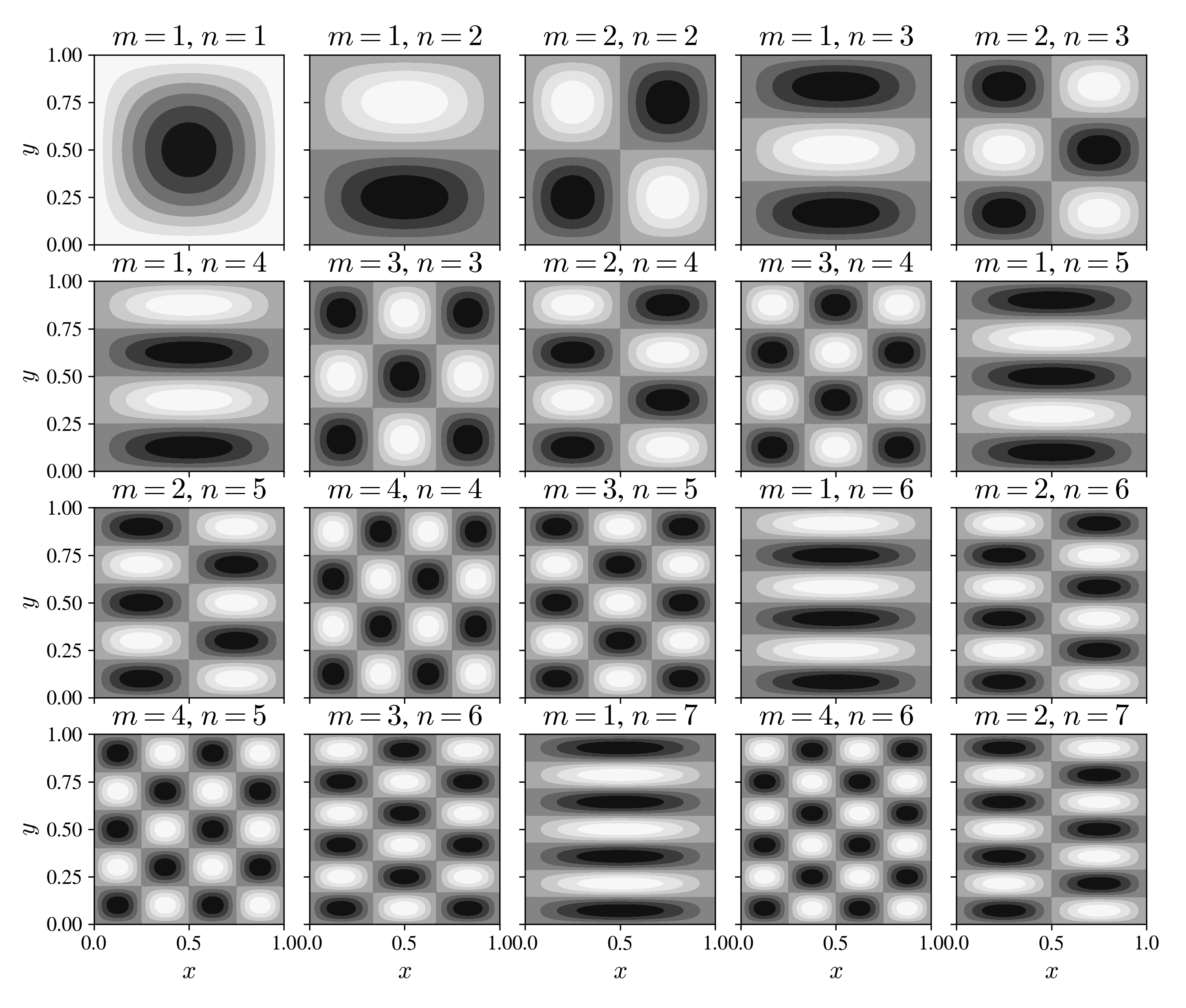
Figure 1: Analytic eigenvectors for the oscillation of a square membrane, ordered by increasing frequency.

III-C Results

The partial differential equation is solved numerically for different damping rates using the meshless RBF-FD [13] method implemented with the Medusa [14] C++ library. A subset of system state snapshots for the 0 damping case that that we use in DMD is shown in the right graphs of Figure 2. The dynamics are disordered due to the non-symmetric position of the initial jolt and do not offer much insight at the first glance. We can use the sum of membrane heights as an observable that reduces the system’s behaviour into a single scalar value to visualise the oscillation and the effect of different damping rates as shown in the left graph of Figure 2.

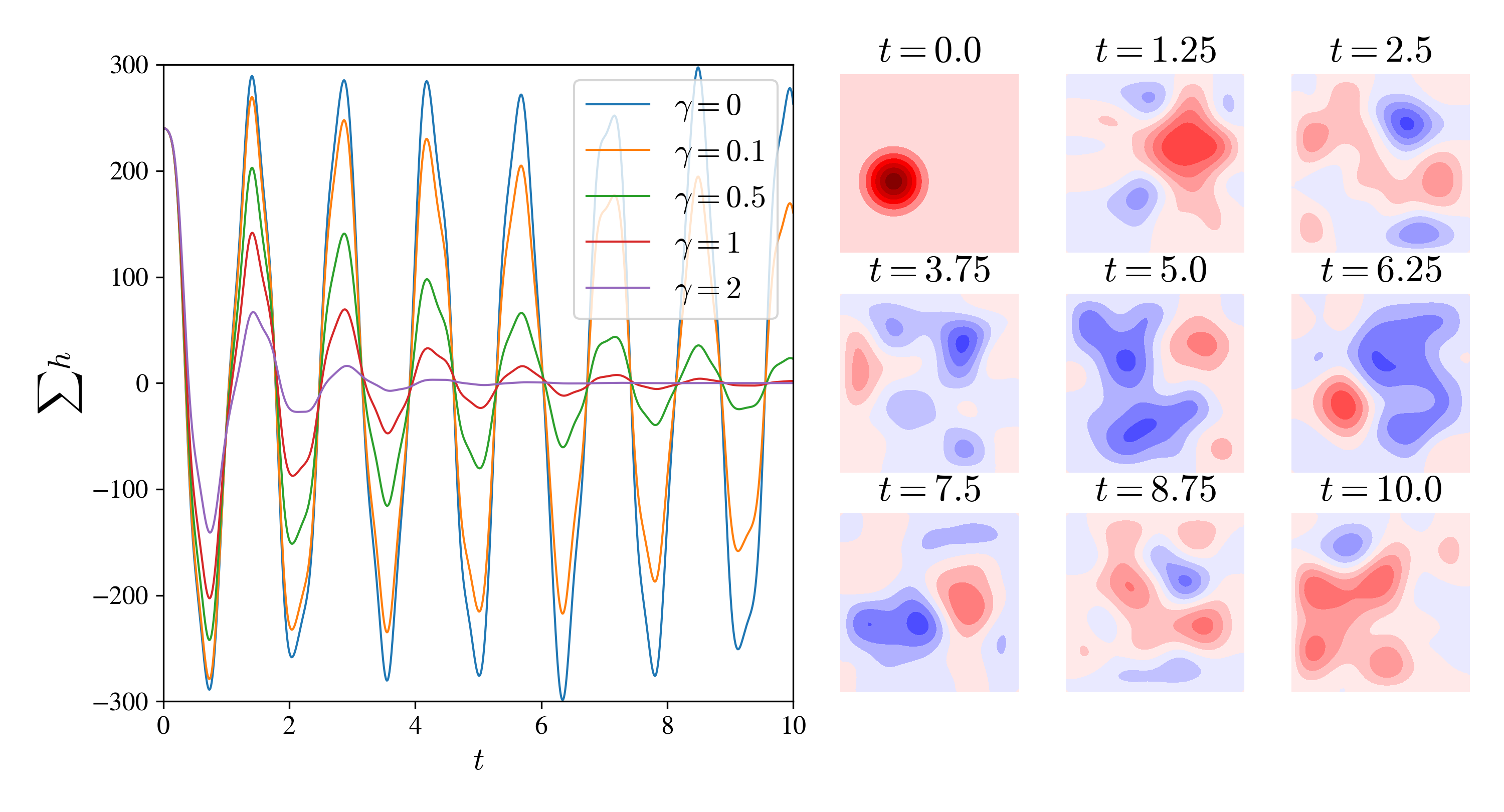
Figure 2: left: The sum of height values provides a simple insight into the system’s behaviour. The time evolution of thus derived observable is shown for different damping rates $\gamma$. right: A selection of snapshots used in the decomposition providing an insight into the system’s behaviour during the observed time. A heat map display is used to visualise the scalar values with blues for negative, white for zero and reds for positive values.

We use DMD on 1000 uniformly sampled snapshots from the interval $t\in[0,10]$ that are composed into the data matrix $\boldsymbol{V}$ with stacking $m=10$. Each snapshot is composed of 3985 height values in computational nodes for the mesh-free partial differential equation solving, which are uniformly positioned within $\Omega$.

The resulting frequencies, calculated from DMD eigenvalues as described in Eq. (2), are shown in the top graph of Figure 3. The results provide a good estimation for the analytic results with sub percent relative error for the first $\sim 30$ modes as shown in the central graph. Estimated frequencies remain good even for the relatively strongly damped $\gamma=1$ case showing promise for eigenfrequency estimation on experimental data obtained from complex objects.

There is a slight inconsistency in the results with a sharp increase in the relative error for the $\gamma=0$ frequencies. We would expect that the least damped case would give the best results but there seems to be an additional non-physical mode at index 11 that has caused a shift in the following frequencies. Fortunately we can use the mode power described in Sec. II-C and shown in the bottom graph of Figure 3 to detect and remove the highlighted spurious mode with a significantly lower strength. It is surprising how little nonsensical modes we identified even though we initially disturbed the membrane in a non-symmetric location and how chaotic the actual system shown in the heat maps of Figure 2 looks to a human observer.

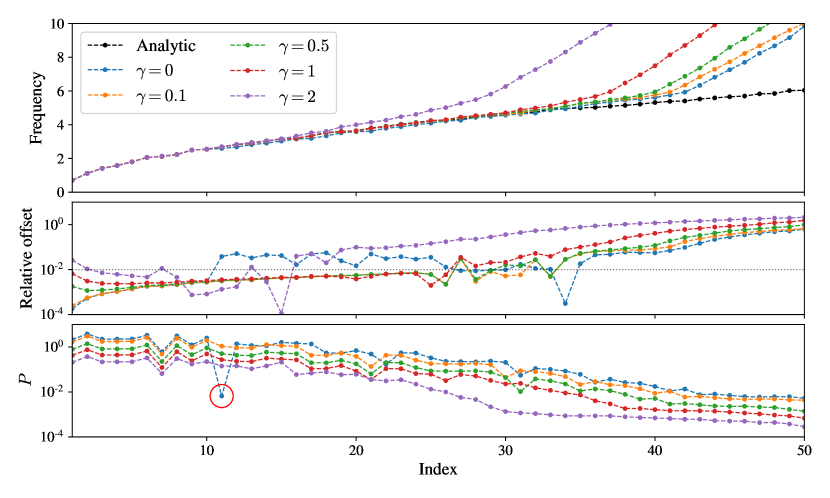
Figure 3: top: Eigenfrequencies calculated with DMD for different damping rates compared to analytic values. centre: The relative error between DMD eigenfrequencies and analytic values for the square membrane. bottom: Mode powers for the calculated DMD modes.

We can also compare the analytic eigenvectors shown in Figure 1 and DMD eigenvectors in Figure 4. The DMD vector positions in the grid are shifted by one compared to the analytic due to the non-oscillatory background mode that is always present in the decomposition of data with non-zero average. Some eigenvectors match almost perfectly while others wildly differ. This might seem inconsistent at the first glance but can be explained with degeneracy in the analytical spectrum. Linear combinations of degenerate eigenvectors still constitute a valid eigenvector. The non-symmetric eigenvector $\varphi_{11}$ can quickly be identified as the one corresponding to the previously mentioned spurious mode.

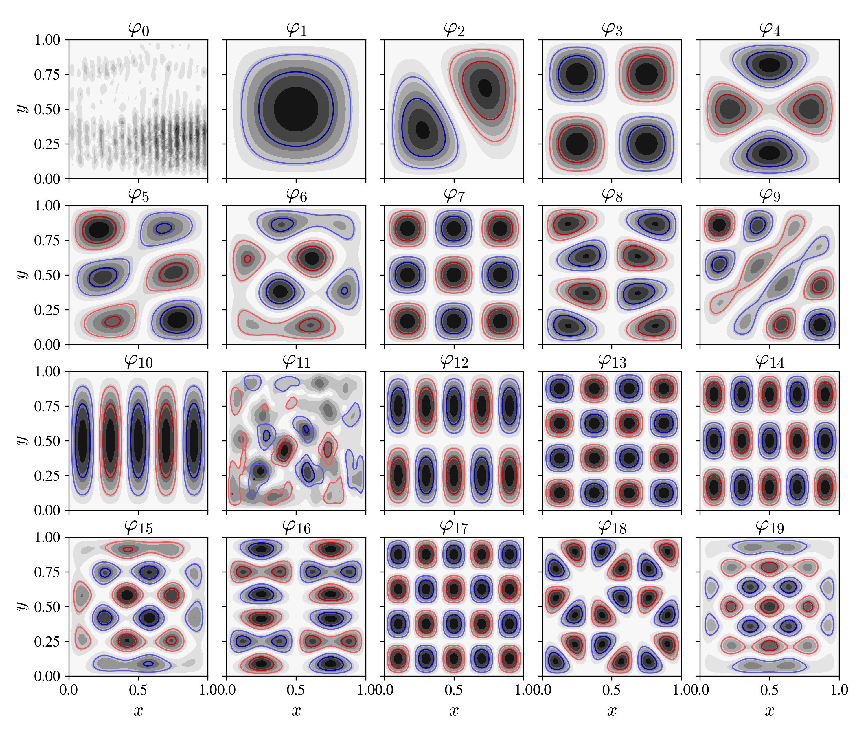
Figure 4: DMD mode eigenvectors ordered by frequency for the $\gamma=0$ case. The positions of modes are shifted by one relative to Figure 3 because of the constant, zero frequency, background mode. The grayscale image displays absolute value with contours ranging from blue to red for the imaginary part.

III-D Oddly shaped membrane

Now that we have shown that DMD can be used to identify inherent oscillatory modes we apply it to an irregularly shaped membrane. The duck-shaped membrane is again disturbed with a Gaussian initial state, resulting in the oscillation shown in Figure 5. This combination of meshless computational nodes, the time evolution of the system, the DMD spectrum, and the DMD eigenvectors ordered by frequency provides a condensed overview of the dynamics and shows how DMD could be used in engineering analysis. The DMD spectrum is a convenient and commonly used display of DMD mode frequency and power in the same graph, which can, when sorted by frequency, be used similarly to the Fourier transform.

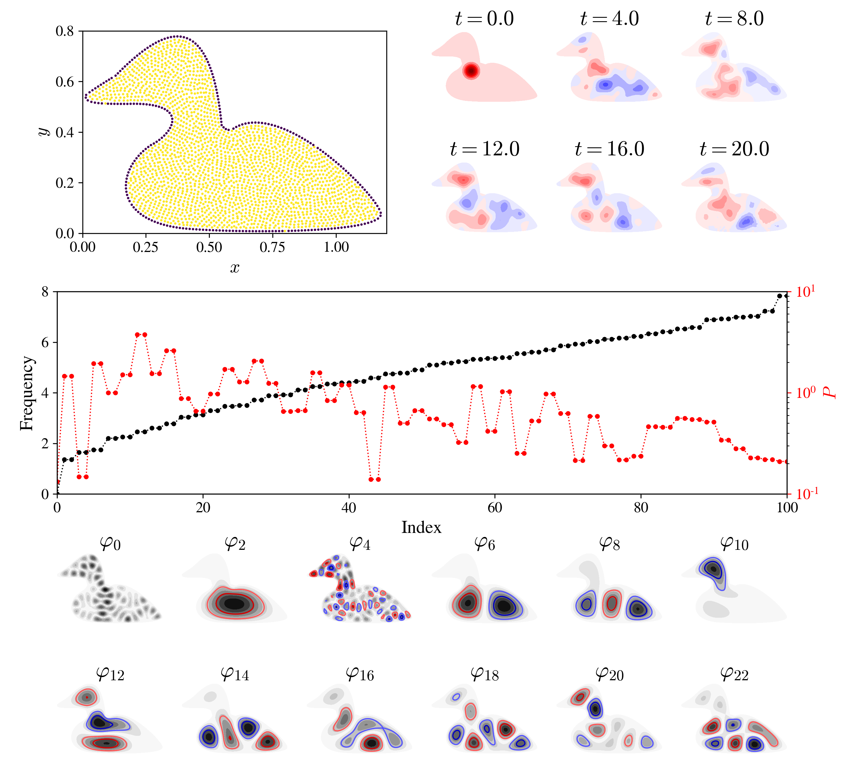
Figure 5: The DMD decomposition applied to a duck-shaped oscillating membrane. top left: Positioning of computational nodes with yellow for interior nodes where we solve the wave equation and purple for boundary nodes with enforced Dirichlet condition. top right: A subset of membrane state snapshots used for DMD. centre: The DMD spectrum showing the frequencies and powers of modes ordered by the former. bottom: Eigenvectors of DMD modes ordered by frequency.

IV Non-Newtonian fluid

The last example is a practical use case for DMD applied to hydrodynamics. We solve, with details available in [15], the system of partial differential equations

$$\divergence\boldsymbol{v} =0,$$ (17)

$$\rho(\partialderivative{\boldsymbol{v}}{t}+\boldsymbol{v}\cdot\gradient{\boldsymbol{v}}) =-\gradient p+\divergence(\eta\gradient\boldsymbol{v})-\boldsymbol{g}\rho\beta T_{\Delta},$$ (18)

$$\rho c_{p}(\partialderivative{T}{t}+\boldsymbol{v}\cdot\gradient{T}) =\divergence(\lambda\gradient T),$$ (19)

$$\eta =\eta_{0}\left(\frac{1}{2}\norm{\gradient{\boldsymbol{v}}+(\gradient{\boldsymbol{v}})^{T}}\right)^{\frac{n-1}{2}}.$$ (20)

with $\boldsymbol{v}$, $T$, $p$, $\rho$, $\boldsymbol{g}$, $\beta$, $T_{\Delta}$, $c_{p}$, $\eta_{0}$, $n$ representing the flow velocity field, temperature field, pressure field, density, gravity, thermal expansion coefficient, temperature offset, heat capacity, viscosity constant and non-Newtonian index respectively.

The system is used to describe the natural convection in an incompressible non-Newtonian fluid. Non-Newtonian fluids have a variable viscosity meaning that the relationship between the shear-strain and the shear-stress is non-linear. We use a simple power-law model to describe the relationship with non-Newtonian power index $n$ as the main parameter of behaviour. Smaller values of $n$ indicate stronger shear-thinning non-Newtonian effects while $n=1$ equals to a normal, Newtonian, fluid.

We will be using the dimensionless Rayleigh number (Ra) that has a similar meaning for natural convection as Reynolds number, meaning stronger dynamics for higher values, as a case parameter, with details unimportant for the demonstration.

The model is solved in a square cavity with differentially heated walls schematically shown in the upper left graph of Figure 6. The left and right walls are kept at a temperature differential causing the fluid to form a vortex as it heats and rises at the right boundary and cools and descends on the left. This circulation is stationary for low Ra with a transition into an oscillatory and later chaotic regime as Ra increases. The upper right graphs in Figure 6 show a selection of system temperature and velocity field snapshots for the oscillatory behaviour at Ra$=10^{6}$. A set of parameters where the transition into the oscillatory behaviour occurs has been identified by Kosec et al. [16] and we use DMD to analyse the differences in dynamics as we push past that point with increasing Ra and decreasing $n$.

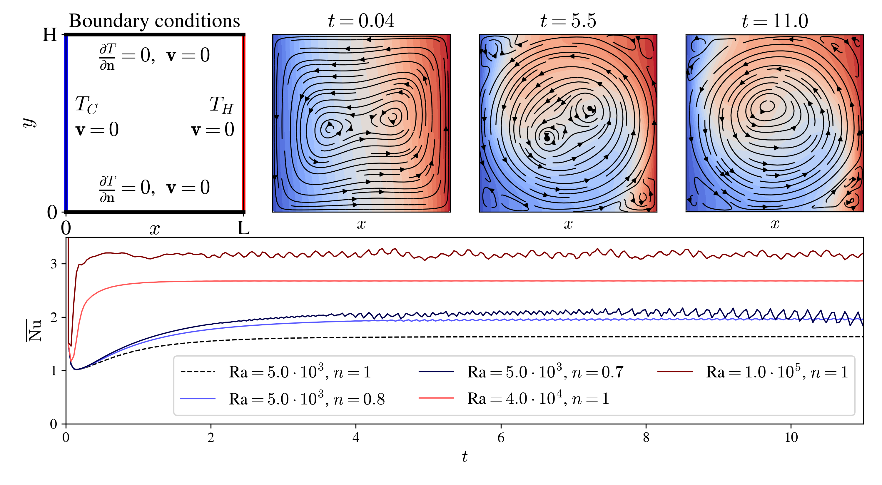
Figure 6: The setup and behaviour for the differentially heated cavity non-Newtonian natural convection case. upper left: The case setup with boundary conditions. upper right: A selection of snapshots sampled from the system with Ra$=10^{6}$ and $n=1$. The red-blue background colour shows the local fluid temperature with added streamlines to illustrate the flow direction. bottom: Time evolution of Nusselt number for different parameters.

As mentioned in the introduction we can use the Nusselt number, shown in the bottom graph of Figure 6, as an observable into the systems behaviour. The system is stationary for Ra$=5\cdot 10^{3}$ and $n=1$ but oscillations occur both when we increase Ra and when we decrease $n$.

We use DMD to decompose the 5 cases utilising 500 snapshots of the system between $t=10$ and $t=11$ with stacking $m=5$. The results are shown in Figure 7a for increasing Ra and Figure 7b for decreasing $n$. The mode power defined in Eq. (12) is used to identify the strongest modes and display the corresponding eigenvectors. The first observation that is common to both modes of spurring the dynamics pertains to the DMD spectrum. The initial stationary case has the vast majority of its power in the first constant mode with others most likely only containing noise. As the intensity of the dynamics increases we get more distinct modes but the power of the background modes also increases as expected with ever wilder dynamics heading towards chaos, where all modes would be present and indistinguishable by power.

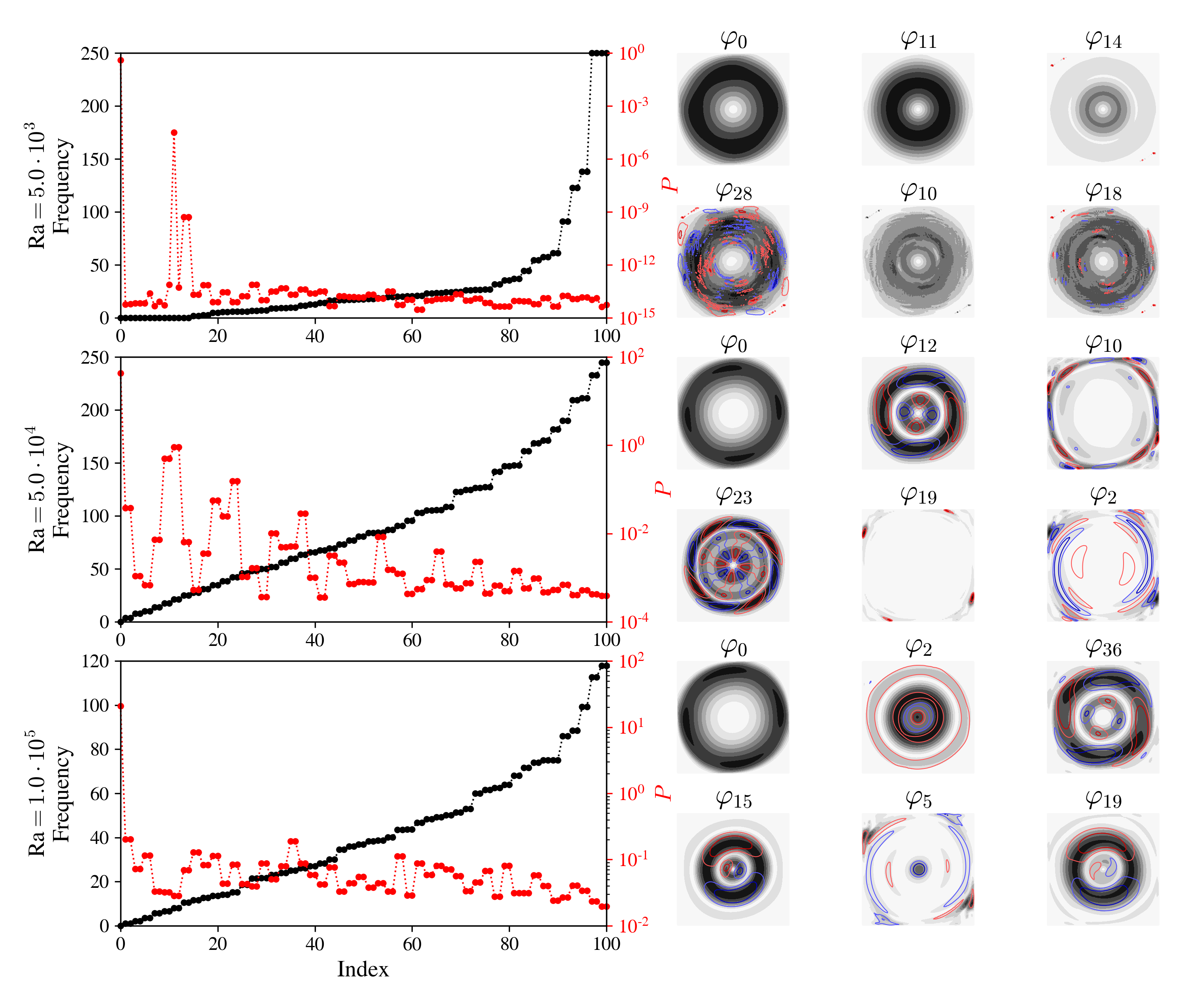
(a) Different Ra, Newtonian $n=1$.

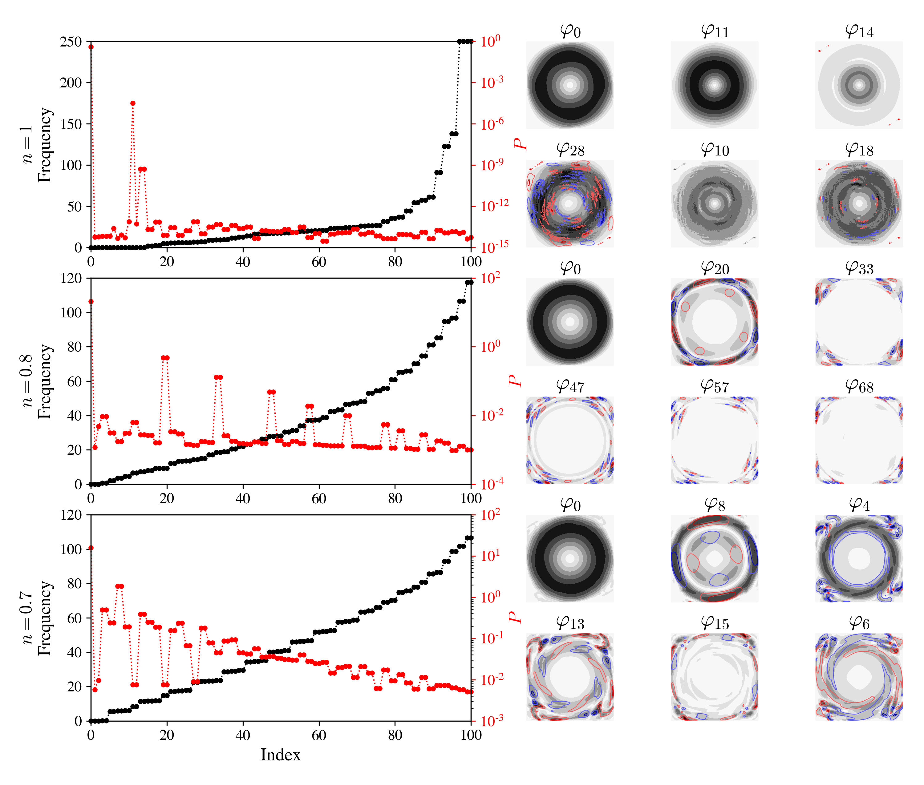
(b) Different non-Newtonian $n$, Ra$=5\cdot 10^{3}$.

Figure 7: The DMD spectra and eigenvectors for the strongest modes.

We can be reasonably certain that the oscillatory dynamics are in fact different for the Ra and $n$ spurred dynamics by using the eigenvectors of DMD modes sorted by power to identify the important parts. The strongest areas are clearly different with eigenvectors for the Ra induced dynamics in Figure 7a present mainly as perturbations to the main central vortex while the modes for the $n$ induced dynamics in Figure 7b point to activity in corners where counter vortices occur. This is consistent with the typical shear-thinning non-Newtonian behaviour where the larger velocity gradients are penalised less providing better conditions for smaller vortices.

V Conclusion

We have presented the algorithm for dynamic mode decomposition and applied it to various test and example cases. The examples progressed from the most basic, where we were able to verify the results agains known closed-form values, towards a concrete hydrodynamics example where DMD provided valuable insight into the system that would be difficult to obtain otherwise. The DMD has proved to be a very practical tool for dynamical system analysis and it is recommended that anyone dealing with hydrodynamics or similarly complex systems should be at least familiar with its fundamentals. The algorithm is only a decade old and has an active community working on extensions for the concept of Koopman operator decomposition and applications for the existing versions of DMD.

References

- [1] T. R. Ricciardi, W. Wolf, R. L. Speth, and P. Bent, “Analysis of noise sources in realistic landing gear configurations through high fidelity simulations,” in AIAA Scitech 2019 Forum, 2019. [Online]. Available: https://arc.aiaa.org/doi/abs/10.2514/6.2019-0003
- [2] J. L. Lumley, “The structure of inhomogeneous turbulent flows,” in Proceedings of the International Colloquium on the Fine Scale Structure of the Atmosphere and its Influence on Radio Wave Propagation, A. M. Yaglam and V. I.Tatarsky, Eds., Moscow, 1967, pp. 166–178.
- [3] C. W. Rowley, “Model reduction for fluids, using balanced proper orthogonal decomposition,” International Journal of Bifurcation and Chaos, vol. 15, no. 03, pp. 997–1013, 2005.
- [4] K. Taira, S. L. Brunton, S. T. M. Dawson, C. W. Rowley, T. Colonius, B. J. McKeon, O. T. Schmidt, S. Gordeyev, V. Theofilis, and L. S. Ukeiley, “Modal analysis of fluid flows: An overview,” AIAA Journal, vol. 55, no. 12, pp. 4013–4041, 2017. [Online]. Available: https://doi.org/10.2514/1.J056060
- [5] P. Holmes, J. L. Lumley, G. Berkooz, and C. W. Rowley, Turbulence, Coherent Structures, Dynamical Systems and Symmetry, 2nd ed., ser. Cambridge Monographs on Mechanics. Cambridge University Press, 2012.
- [6] P. J. Schmid, “Dynamic mode decomposition of numerical and experimental data,” Journal of Fluid Mechanics, vol. 656, p. 5–28, 2010.
- [7] J. Proctor and P. Welkhoff, “Discovering dynamic patterns from infectious disease data using dynamic mode decomposition,” International health, vol. 7, pp. 139–45, 03 2015.
- [8] J. Grosek and J. N. Kutz, “Dynamic mode decomposition for real-time background/foreground separation in video,” arXiv e-prints, p. arXiv:1404.7592, Apr. 2014.
- [9] C. W. Rowley, I. Mezić, S. Bagheri, P. Schlatter, and D. S. Henningson, “Spectral analysis of nonlinear flows,” Journal of Fluid Mechanics, vol. 641, p. 115–127, 2009.
- [10] J. H. Tu, C. W. Rowley, D. M. Luchtenburg, S. L. Brunton, and J. N. Kutz, “On dynamic mode decomposition: Theory and applications,” Journal of Computational Dynamics, vol. 1, no. 2, pp. 391–421, 2014.
- [11] J. Tu, “Dynamic mode decomposition: Theory and applications,” Ph.D. dissertation, Princeton University, sep 2013.
- [12] J. N. Kutz, S. L. Brunton, B. W. Brunton, and J. L. Proctor, Dynamic Mode Decomposition: Data-Driven Modeling of Complex Systems, ser. Other Titles in Applied Mathematics. Society for Industrial and Applied Mathematics, 2016. [Online]. Available: https://books.google.si/books?id=wbedDAEACAAJ
- [13] A. I. Tolstykh and D. A. Shirobokov, “On using radial basis functions in a “finite difference mode” with applications to elasticity problems,” Computational Mechanics, vol. 33, no. 1, pp. 68–79, Dec 2003. [Online]. Available: https://doi.org/10.1007/s00466-003-0501-9
- [14] J. Slak and G. Kosec, “Medusa: A c++ library for solving pdes using strong form mesh-free methods,” ACM Trans. Math. Softw., vol. 47, no. 3, Jun. 2021. [Online]. Available: https://doi.org/10.1145/3450966
- [15] M. Rot and G. Kosec, “Refined rbf-fd analysis of non-newtonian natural convection,” 2022. [Online]. Available: https://arxiv.org/abs/2202.08095
- [16] G. Kosec and B. Šarler, “Solution of a low prandtl number natural convection benchmark by a local meshless method,” International Journal of Numerical Methods for Heat & Fluid Flow, vol. 23, p. 22, 01 2013.