Multi-Objective Multi-Agent Planning for Discovering and Tracking Multiple Mobile Objects

Abstract

We consider the online planning problem for a team of agents to discover and track an unknown and time-varying number of moving objects from onboard sensor measurements with uncertain measurement-object origins. Since the onboard sensors have a limited field-of-view, the usual planning strategy based solely on either tracking detected objects or discovering unseen objects is inadequate. To address this, we formulate a new information-based multi-objective multi-agent control problem, cast as a partially observable Markov decision process (POMDP). The resulting multi-agent planning problem is exponentially complex due to the unknown data association between objects and multi-sensor measurements; hence, computing an optimal control action is intractable. We prove that the proposed multi-objective value function is a monotone submodular set function, which admits low-cost suboptimal solutions via greedy search with a tight optimality bound. The resulting planning algorithm has a linear complexity in the number of objects and measurements across the sensors, and quadratic in the number of agents. We demonstrate the proposed solution via a series of numerical experiments with a real-world dataset.

I Introduction

Recent advancements in robotics have inspired applications that use low-cost mobile sensors (e.g., drones), ranging from vision-based surveillance, threat detection via source localisation, search and rescue, to wildlife monitoring [23]. At the heart of these applications is Multi-Object Tracking (MOT)—the task of estimating an unknown and time-varying number of objects and their trajectories from sensor measurements with unknown data association (i.e., unknown measurement-to-object origin). Further, MOT is fundamental for autonomous operation as it provides awareness of the dynamic environment in which the agents operate. Although a single agent can be tasked with MOT, such a system is limited by observability, computing resources, and energy. Using multi-agents alleviates these problems, improves synergy, and affords robustness to failures. Realising this potential requires the multi-agents to collaborate and operate autonomously.

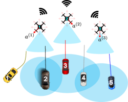
Figure 1: An unmanned aerial vehicles (UAV) team tracking multiple vehicles with limited FoV sensors and unknown measurements-to-objects associations.

In this work, we consider the challenging problem of coordinating multiple limited field-of-view (FoV) agents to simultaneously seek undetected objects and track detected objects (see Fig. 1). Tracking involves estimating the trajectories of the objects and maintaining their provisional identities or labels [42]. Trajectories are important for capturing the behaviour of the objects while their labels provide the means for distinguishing individual trajectories and for human/machine users to communicate information on the relevant trajectories. A single agent with an on-board sensor (e.g., a camera) invariably has a limited FoV [43], and hence, only observes part of the scene at any given time. As a result, a team of multiple agents is often implemented to improve coverage of the surveillance area [44, 45, 46, 47]. However, MOT with multiple limited FoV sensors still encountered several challenges, such as occlusions, missed detections, false alarms, identity switches and track fragmentation [25].

Discovering undetected objects and tracking detected objects are two competing objectives due to the limited FoVs of the sensors (e.g. cameras, antenna, and radar) and the random appearance/disappearance of objects. On one hand, following only detected objects to track them accurately means that many undetected objects could be missed. On the other hand, leaving detected objects to explore unseen regions for undetected objects will lead to track loss. Thus, the problem of seeking undetected objects and tracking detected objects is a multi-objective optimisation problem.

Even for standard state-space models, where the system state is a finite-dimensional vector, multi-agent planning with multiple competing objectives is challenging due to complex interactions between agents resulting in combinatorial optimisation problems [34]. In MOT, where the system state (and measurement) is a set of vectors, the problem is further complicated due to: i) the unknown and time-varying number of trajectories; ii) missing and false detections; and iii) unknown data association (measurement-to-object origins) [20]. Most critically for real-world applications, multi-agent control actions must be computed online and in a timely manner.

Model predictive control (MPC) is an effective approach to stochastic control and is widely used in real-world applications [11], compared to meta-heuristics (or bio-inspired) techniques such as genetic algorithms and particle swarm optimisation [49], which are expensive for real-time applications in dynamic environments such as MOT. The MPC problem can be cast as a partially observed Markov decision process (POMDP), which has been gaining significant interest as a real-time planning approach [3]. The cooperation problem amongst agents can be formulated as a decentralised POMDP (Dec-POMDP), whose exact solutions are NEXP-hard [2]. Moreover, for multi-agent Dec-POMDP, the action and observation space grows exponentially with the number of agents [50], and hence not suitable for real-time applications. So far, the centralised Multi-agent POMDP approach [21] offers a more tractable alternative for coordinating multiple agents  [7, 33], and hence is adopted in this work.

Computing optimal control actions for MOT within a POMDP requires a suitable framework that provides a multi-object density for the information state. Amongst various MOT algorithms, we adopt the labelled random finite set (RFS) filtering framework because it provides a multi-object filtering density that contains all information about the current set of trajectories and accommodates the time-varying set of trajectories of mobile objects. Single-agent planning with RFS filters has been studied in with an unlimited FoV [28, 13] and extended to multi-agent planning using distributed fusion techniques [33]. However, these multi-agent planning methods are only suitable when the agents have an unlimited detection range [25]. A multi-agent POMDP with an RFS filter was proposed in [7] for searching and localisation, but not tracking.

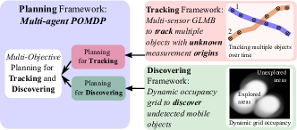
Figure 2: A schematic of the proposed planning approach.

To achieve competing discovery and tracking objectives, we propose a POMDP with a multi-objective value function consisting of information gains for both detected and undetected objects, as illustrated in Fig. 2. A simple solution for competing objective functions is to weigh and add them together. However, meaningful weighting parameters are difficult to determine. A multi-objective optimisation approach naturally provides a meaningful trade-off between competing objectives. To the best of our knowledge, multi-agent planning for MOT with a multi-objective value function has not been investigated. The first multi-objective POMDP with a localisation RFS filter was proposed in [36] for a sensor selection problem.

For MOT and the information state, we use the multi-sensor Generalised Labelled Multi-Bernoulli (MS-GLMB) filter [30], which exhibits linear computational complexity in the total number of measurements across the sensors. For path planning, we use the centralised Multi-Agent POMDP (MPOMDP) framework [21] with the GLMB filter. Further, for the value function, we use the differential entropy [6, pp.243] of the Labelled Multi-Bernoulli (LMB) density [27] that matches the first moment of the information state. In particular, we derive an analytic expression for this differential entropy, which can be computed with linear complexity in the number of hypothesised objects, and show that the resulting multi-objective value function is monotone submodular. Consequently, this enables us to exploit low-cost greedy search to solve the optimal control problem with a tight optimality bound. In summary, the main contributions are:

• a multi-objective POMDP formulation for multi-agent planning to search and track multiple objects;

• an efficient multi-agent path planning algorithm based on multi-object differential entropy with linear complexity in the objects, measurements across the sensors, and quadratic in the number of agents.

The proposed method is evaluated using the CRAWDAD taxi dataset [8] on multi-UAVs control for searching and tracking an unknown and time-varying number of taxis in downtown San Francisco. For performance benchmarking, our preliminary work in  [24] is used as the ideal or best-case scenario where data association is known.

The remainder of this paper is organised as follows. Section II provides relevant background for our MOT and planning framework. Section III presents our proposed multi-objective value function for the control of the multi-agent to simultaneously track and discover objects. Section IV evaluates our proposed method on a real-world dataset. Section V summarises our contributions and discusses future directions.

II Background

This section presents the problem statement and provides the necessary background on MPOMDP and MS-GLMB filtering. We use notation in accordance with [32]. Lowercase letters (e.g., $x,\boldsymbol{x}$) denote vectors, uppercase letters (e.g., $X,\boldsymbol{X}$) denote finite sets, while spaces are denoted by blackboard uppercase letters (e.g., $\mathbb{X},\mathbb{L}$). Vectors augmented with labels, finite sets of labelled vectors, and the corresponding spaces are bolded (e.g., $\boldsymbol{x,X}$, $\boldsymbol{\mathbb{X}},\boldsymbol{\mathbb{U}}$) to distinguish them from unlabelled ones. For a given set $S$, $|S|$ $,1_{S}(\cdot)$, $\delta_{S}[\cdot]$ denote, respectively, the cardinality, indicator function, and (generalised) Kronecker delta function, of $S$ ($\delta_{S}[X]=1$, if $X=S$, and zero otherwise). For a function $f$, its multi-object exponential $f^{X}$ is defined as $\prod_{x\in X}f(x)$, with $f^{\emptyset}=0$. The inner product $\int f(x)g(x)dx$ is written as $\langle f,g\rangle$, while the superscript ^† denotes the transpose of a vector/matrix. For compactness, the subscript for time $k$ is omitted, and subscripts for times $k-1$ and $k+1$ are abbreviated ‘$-$’ and ‘$+$’.

II-A Problem statement

Consider a team of agents, equipped with limited-FoV sensors that record detections with unknown data association (measurement-to-object origins), monitoring an unknown and time-varying number of objects. The agents can self-localise and communicate (e.g., sending observations) to a central node that determines/issues control actions [7]. For each agent $n\mathcal{\in N}=\{1,\dots,|\mathcal{N}|\}$, its state space, (discrete) control action space, and observation space, are denoted respectively by $\mathbb{U}^{(n)}$, $\mathbb{A}^{(n)}$, and $\mathbb{Z}^{(n)}$. We define the common observation space for all agents as $\boldsymbol{\mathbb{Z}}\triangleq\uplus_{n\in\mathcal{N}}\mathbb{Z}^{(n)}\times\{n\}$.

Each object is described by a labelled state $\boldsymbol{x}=(x,\ell)\in\boldsymbol{\mathbb{X}}\triangleq\mathbb{X}\times\mathbb{L}$, consisting of a time-varying attribute $x\in\mathbb{X}$, and a time-invariant discrete label $\ell\in\mathbb{L}$. To capture the time-varying number of trajectories, the multi-object state at any given time is represented by the set $\boldsymbol{X}$ of distinctly labelled states of the objects [32], [51]. Thus, the multi-object state space $\boldsymbol{\mathcal{X}}$ is the partition matroid of $\boldsymbol{\mathbb{X}}$. A partition matroid of a space $\boldsymbol{\mathbb{S}}=\mathbb{S}\times\mathbb{I}$, with $\mathbb{I}$ a discrete set, is the class of subsets of $\boldsymbol{\mathbb{S}}$, defined by [5]:

$$\boldsymbol{\mathcal{S}}\triangleq\{\boldsymbol{S}\subseteq\boldsymbol{\mathbb{S}}:|\boldsymbol{S}\cap(\mathbb{S}\times\{i\})|\leq 1,~{}\forall i\in\mathbb{I}\}.$$

Each member of the partition matroid $\boldsymbol{\mathcal{S}}$ has distinct indices.

Our goal is to coordinate the team of agents to search and track a time-varying and unknown number of moving objects. The main challenges are: i) misdetection of objects due to the limited FoVs; ii) lack of prior information about the changing number of objects and their locations; iii) unknown data association; and iv) the computational resources required to determine multi-agent control actions in a timely manner.

II-B MPOMDP for Multi-Object Tracking

A random finite set (RFS) model [19, 17] succinctly captures the random nature of the multi-object states and offers a suitable concept of multi-object density for the POMDP’s information state. Specifically, an RFS of a space $\mathbb{X}$ is a random variable taking values in the class $\mathcal{X}$ of finite subsets of $\mathbb{X}$, and is commonly characterised by Mahler’s multi-object density [19] (see also subsection III-A). Since the elements of a multi-object state are distinctly labelled, we model the multi-object state as a labelled RFS–an RFS of $\boldsymbol{\mathbb{X}}$ such that instantiations have distinct labels [32], i.e., a random variable taking values in the partition matroid $\boldsymbol{\mathcal{X}}$.

The multi-object MPOMDP considered in this work can be characterised by the tuple $(\mathcal{N},H,\boldsymbol{\mathcal{X}},\boldsymbol{\mathcal{Z}},\mathcal{\mathbb{A}},\boldsymbol{f},\boldsymbol{g},\boldsymbol{\varrho})$, where

• $\mathcal{N}$ is the finite set of agent labels;

• $H$ is the look-ahead time horizon;

• $\boldsymbol{\mathcal{X}}$ is the multi-object state space (partition matroid of $\boldsymbol{\mathbb{X}}$);

• $\boldsymbol{\mathcal{Z}}$ is the multi-object observation space (class of finite subsets of $\boldsymbol{\mathbb{Z}}$);

• $\mathbb{A}=\mathbb{A}^{(1)}\times...\times\mathbb{A}^{(|\mathcal{N}|)}$ is multi-agent action space;

• $\boldsymbol{f}(\boldsymbol{X}|\boldsymbol{X}_{-},a_{-})$ is the transition density for $\boldsymbol{X},\boldsymbol{X}_{-}\in\boldsymbol{\mathcal{X}}$, and action $a_{-}\in\mathbb{A}$ has been taken;

• $\boldsymbol{g}(\boldsymbol{Z}|\boldsymbol{X},a_{-})$ is the likelihood of observation $\boldsymbol{Z}\in\boldsymbol{\mathcal{Z}}$ given $\boldsymbol{X}\in\boldsymbol{\mathcal{X}}$, and action $a_{-}\in\mathbb{A}$ has been taken;

• $\boldsymbol{\varrho}(\boldsymbol{Z},\boldsymbol{X},a_{-})$ is the immediate reward for observing $\boldsymbol{Z}\in\boldsymbol{\mathcal{Z}}$ from $\boldsymbol{X}\in\boldsymbol{\mathcal{X}}$, after action $a_{-}\in\mathbb{A}$ has been taken.

The agents are coordinated at each time $k$ via the multi-agent action $a=(a^{(1)},...,a^{(|\mathcal{N}|)})\in\mathbb{A}$, which prescribes a state for each agent $n$ at time $k+1$, where it collects the multi-object observation $\boldsymbol{Z}_{+}^{(n)}\subset\mathbb{Z}^{(n)}$ from the multi-object state $\boldsymbol{X}_{+}$ that evolved from $\boldsymbol{X}$ according to the multi-object transition density $\boldsymbol{f}_{+}(\boldsymbol{X}_{+}|\boldsymbol{X},a)$. The multi-agent multi-object observation $\boldsymbol{\,Z}_{+}\in\boldsymbol{\mathcal{Z}}$ is given by $\uplus_{n=1}^{|\mathcal{N}|}\boldsymbol{Z}_{+}^{(n)}$, or equivalently the $|\mathcal{N}|$-tuple $(\boldsymbol{Z}_{+}^{(1)},\dots,\boldsymbol{Z}_{+}^{(|\mathcal{N}|)})$, and has likelihood $\boldsymbol{g}_{+}(\boldsymbol{Z}_{+}|\boldsymbol{X}_{+},a)$. The specifics of $\boldsymbol{f}_{+}$ and $\boldsymbol{g}_{+}$ are detailed in Subsection (II-C).

The information state of the MPOMDP at time $j>1$ is the (labelled) multi-object filtering density $\boldsymbol{\pi}_{a_{j-1},j}(\cdot|\boldsymbol{Z}_{j})$, which contains all information about the multi-object state given the observation history [32]. For notational convenience, we indicate dependence only on the latest control action and observation. Starting with the initial prior $\boldsymbol{\pi}_{a_{0},1}$, the information state $\boldsymbol{\pi}_{a_{j-1},j}(\cdot|\boldsymbol{Z}_{j})$ is propagated via Bayes recursion:

$$\!\!\!\!\boldsymbol{\pi}_{a_{j-1},j}(\boldsymbol{\boldsymbol{X}}_{j}) =\int\!\!\boldsymbol{f}_{j}(\boldsymbol{X}_{j}|\boldsymbol{X},a_{j-1})\boldsymbol{\pi}_{a_{j-2},j-1}\!\left(\boldsymbol{X}\right)\delta\boldsymbol{X},$$ (1)

$$\!\!\!\!\boldsymbol{\pi}_{a_{j-1},j}(\boldsymbol{\boldsymbol{X}}_{j}|\boldsymbol{Z}_{j}) =\frac{\boldsymbol{g}_{j}(\boldsymbol{Z}_{j}|\boldsymbol{\boldsymbol{X}}_{\!j},a_{j-1})\boldsymbol{\pi}_{a_{j-1},j}(\boldsymbol{\boldsymbol{X}}_{j})}{\boldsymbol{g}_{j}(\boldsymbol{Z}_{j}|a_{j-1})},$$ (2)

where $\boldsymbol{g}_{j}(\boldsymbol{Z}_{j}|a_{j-1})=\int\boldsymbol{g}_{\!j}(\boldsymbol{Z}_{j}|\boldsymbol{\boldsymbol{X}}_{\!j},a_{j-1})\boldsymbol{\pi}_{a_{j-1},j}(\boldsymbol{\boldsymbol{X}}_{\!j})\delta\boldsymbol{\boldsymbol{X}}_{j}$ is the predictive likelihood under action $a_{j-1}$, and the integral is Mahler’s set integral (see also Subsection III-A for details).

A POMDP seeks the control action sequence $a_{k:k+H-1}$ that maximises a value function $V\big{(}a_{k:k+H-1}\big{)}$ constructed from the information states and immediate rewards over horizon $H$, e.g., the expected sum of immediate rewards

$$V\big{(}a_{k:k+H-1}\big{)}=$$ (3)

$$\sum_{j=k+1}^{k+H}\int\!\!\!\int\!\!\boldsymbol{\varrho}_{j}\!\left(\boldsymbol{Z},\boldsymbol{X}\!,a_{j-1}\right)\boldsymbol{\pi}_{\!a_{j-1},j}(\boldsymbol{X}|\boldsymbol{Z})\boldsymbol{g}_{j}(\boldsymbol{Z}|a_{j-1})\delta\boldsymbol{X}\delta\boldsymbol{\boldsymbol{Z}}\!.$$

In general, the value function (3) cannot be evaluated analytically, while numerical evaluations are intractable [52]. An approximate strategy is to assume $a_{j}=a$ for $j=k:k+H-1$, and determine the action $a$ that optimises the resulting value function, but only apply this action for $M<H$ time steps [23], [52]. The process is then repeated at time $M+1$. However, for multi-object multi-agent problems, this approximation strategy is still too computationally intensive [18].

A computationally tractable value function is based on the notion of Predicted Ideal Measurement Set (PIMS) [20]. Using the information state $\boldsymbol{\pi}_{a_{k-1},k}(\cdot|\boldsymbol{Z}_{k})$ at time $k$, we first compute the multi-object prediction density

$$\widehat{\boldsymbol{\pi}}_{a,j}(\boldsymbol{\boldsymbol{X}}_{\!j}) =\int\!\prod_{i=k+1}^{j}\!\!\boldsymbol{f}_{\!i}(\boldsymbol{X}_{\!i}|\boldsymbol{X}_{\!i-1},a)\boldsymbol{\pi}_{a_{k-1},k}\!\left(\boldsymbol{X}_{\!k}\right)\delta\boldsymbol{X}_{\!k:j-1},$$

from which the predicted multi-object state $\boldsymbol{\boldsymbol{\widehat{X}}}_{a,j}$ is determined via some multi-object estimator. The PIMS $\widehat{\boldsymbol{Z}}_{a,j}$ is the multi-object observation of $\boldsymbol{\boldsymbol{\widehat{X}}}_{a,j}$ without noise, clutter, or misdetection, after action $a$ has been applied at times $k$ to $k+j-1$ [20]. The PIMS-based value function is defined as

$$\!\!\!V(a)=\sum_{j=k+1}^{k+H}\int\!\boldsymbol{\varrho}_{j\!}\big{(}\widehat{\boldsymbol{Z}}_{a,j},\boldsymbol{\boldsymbol{X}}_{\!j},a\big{)}T\boldsymbol{(\pi}_{a,j}(\boldsymbol{X}_{\!j}|\widehat{\boldsymbol{Z}}_{a,j}))\delta\boldsymbol{\boldsymbol{X}}_{\!j},\!\!$$ (4)

where $T$ is some transformation of the information state, e.g., a distribution constructed from its moments.

II-C MS-GLMB Filtering

II-C1 Multi-Object Dynamic Model

The multi-object transition density $\boldsymbol{f}_{+}$ captures the motions and births/deaths of objects. At time $k$, an object with state $\boldsymbol{x}=(x,\ell)\in\boldsymbol{X}$ either survives to the next time with probability $P_{S,+}(\boldsymbol{x})$ or dies with probability $1-P_{S,+}(\boldsymbol{x})$ [32]. Conditional on survival it takes on the state $\boldsymbol{x}_{+}=(x_{+},\ell_{+})$ according to the transition density $f_{S,+}(x_{+}|x,\ell)\delta_{\ell}[\ell_{+}]$, where $\delta_{\ell}[\ell_{+}]$ ensures the label remains the same. In addition, an object with state $\boldsymbol{x}_{+}=(x_{+},\ell_{+})$ is born at time $k+1$ with probability $P_{B,+}(\ell_{+})$, and its unlabelled state $x_{+}$ is distributed according to the probability density $f_{B,+}(\cdot,\ell)$. It is standard practice to assume that, conditional on the current multi-object state, objects are born or displaced at the next time, independently of one another [20]. For the search and track problem considered here, the objects themselves are not influenced by the multi-agent actions, and hence the multi-object transition density $\boldsymbol{f}_{+}(\boldsymbol{X}_{+}|\boldsymbol{X})$ is independent of $a$. This also implies the independence of agent $n$’s observation $\boldsymbol{Z}^{(n)}$ from other agents’ actions. An explicit expression for $\boldsymbol{f}_{+}\!\left(\boldsymbol{X}_{+}|\boldsymbol{X}\right)$ based on the described model can be found in [32], though this is not required in this work.

II-C2 Multi-Object Observation Model

The multi-object observation likelihood $\boldsymbol{g}$ captures detections/misdections, false alarms (or clutter), and data association uncertainty. Given a multi-object state $\boldsymbol{X}$, each $\boldsymbol{x}\in\boldsymbol{X}$ has probability $P_{D}^{(n)}(\boldsymbol{x},u^{(n)})$ of being detected by agent $n$ with state $u^{(n)}$, and generates an observation $\boldsymbol{z}=(z,n^{\prime})\in\boldsymbol{\mathbb{Z}}$ with likelihood [18]:

$$g^{(n)}(\boldsymbol{z}|\boldsymbol{x},u^{(n)})=\delta_{n}[n^{\prime}]g^{(n)}(z|\boldsymbol{x},u^{(n)}),$$

or missed with probability $1-P_{D}^{(n)}(\boldsymbol{x},u^{(n)})$. The term $\delta_{n}[n^{\prime}]$ ensures that detections recorded by agent $n$ are tagged with label $n$. The observation set $\boldsymbol{Z}^{(n)}$, collected by this agent, is formed by the superposition of the (object-originated) detections and Poisson clutter with intensity

$$\kappa^{(n)}(\boldsymbol{z}|u^{(n)})=\delta_{n}[n^{\prime}]\kappa^{(n)}(z|u^{(n)}).$$

It is standard practice to assume that conditional on $\boldsymbol{X}$, detections are independent of each other and clutter [19], and that the observations obtained by individual agents are independent [29].

Remark 1

Since the multi-agent state is determined by the control action $a=(a^{(1)},...,a^{(|\mathcal{N}|)})$, we indicate this dependence by writing $P_{D}^{(n)}(\boldsymbol{x},a^{(n)})\triangleq P_{D}^{(n)}(\boldsymbol{x},u^{(n)})$, $\kappa^{(n)}(\boldsymbol{z}|a^{(n)})\triangleq\kappa^{(n)}(\boldsymbol{z}|u^{(n)})$, and $g^{(n)}(\boldsymbol{z}|\boldsymbol{x},a^{(n)})\triangleq g^{(n)}(\boldsymbol{z}|\boldsymbol{x},u^{(n)})$, unless otherwise stated.

Due to the unknown data association, it is necessary to consider all multi-agent association maps, i.e., combinations of measurement-to-object origins. More concisely, a multi-agent association map $\gamma$ is an $|\mathcal{N}|$-tuple of positive 1-1 maps

$$\gamma^{\left(n\right)}\!:\mathbb{L}\rightarrow\{-1{\textstyle:}|\boldsymbol{Z}^{\left(n\right)}|\},\> n=1,...,|\mathcal{N}|,$$

where $\gamma^{\left(1\right)}(\ell)=...=\gamma^{\left(|\mathcal{N}|\right)}(\ell)=-1$ if label $\ell$ is dead/unborn, $\gamma^{\left(n\right)}(\ell)=0$ if object $\ell$ is not detected by agent $n$, and $\gamma^{\left(n\right)}(\ell)>0$ if object $\ell$ generates observation $\boldsymbol{z}_{\gamma^{\left(n\right)}(\ell)}$ at agent $n$ [30]. The positive 1-1 property ensures each observation from agent $n$ originates from at most one object. The space of all such multi-agent associations is denoted as $\Gamma$, and the set $\mathcal{L}(\gamma)\triangleq\{\ell\in\mathbb{L}:\gamma^{\left(1\right)}(\ell),...,\gamma^{\left(|\mathcal{N}|\right)}(\ell)\geq 0\}$ is called the live labels of $\gamma$. It is assumed that conditional on the multi-object state, the measurements from individual agents are independent (i.e., there is no interference among agents in the observation process) [29]. An explicit expression for $\boldsymbol{g}\left(\boldsymbol{Z}|\boldsymbol{\boldsymbol{X}},a\right)$ based on the described model can be found in [30], though this expression is not needed in this work.

II-C3 MS-GLMB Filter

The Bayes recursion (1)-(2) admits an analytical information state (multi-object filtering density) in the form of a GLMB [32]

$$\boldsymbol{\pi}\left(\boldsymbol{X}\right)=\sum_{I,\xi}w^{\left(I,\xi\right)}\delta_{I}[\mathcal{L}\left(\boldsymbol{X}\right)]\left[p^{(\xi)}\right]^{\boldsymbol{X}},$$ (5)

where: $\mathcal{L}\left(\boldsymbol{X}\right)$ denotes the labels of $\boldsymbol{X}$; each $I$ is a finite subset of $\mathbb{L}$; each $\xi$ is a history $\gamma_{1:k}$ of multi-agent association maps up to the current time; each $w^{\left(I,\xi\right)}$ is non-negative such that $\sum_{I,\xi}w^{\left(I,\xi\right)}=1$; and each $p^{\left(\xi\right)}\left(\cdot,\ell\right)$ is a probability density on the attribute space $\mathbb{X}$. Note that the traditional GLMB form involves the distinct label indicator $\delta_{\left|\boldsymbol{X}\right|}\left[\left|\mathcal{L}\left(\boldsymbol{X}\right)\right|\right]$, which is not needed here since the multi-object state space is the partition matroid $\boldsymbol{\mathcal{X}}$. For convenience, we abbreviate the GLMB in (5) by the set of components, i.e., $\boldsymbol{\pi}\triangleq\left\{\left(w^{\left(I,\xi\right)},p^{\left(\xi\right)}\right)\right\}$.

Under the standard multi-object system model [19] described above, the Bayes recursion propagates a GLMB information state $\boldsymbol{\pi}$ to the next GLMB information state

$$\boldsymbol{\pi}_{a,+}=\Omega\left(\boldsymbol{\pi};\boldsymbol{Z}_{+},a\right),$$ (6)

where $\Omega$ denotes the MS-GLMB recursion operator (which depends on the multi-object model parameters $P_{B},f_{B}$, $P_{S}$, $f_{S}$, $\kappa^{\left(n\right)}$, $P_{D}^{(n)}$, and $g^{\left(n\right)}$, $n\in\mathcal{N}$, see [30] for the actual mathematical expression). Thus, starting with an initial GLMB, all subsequent information states are GLMBs. In practice, the number of GLMB components grows with time and truncation is needed to curb this growth [30].

III Multi-Agent Path Planning for Multi-Object

This section presents our approach to multi-agent planning, with limited FoV sensors, for searching and tracking an unknown and time-varying number of objects, as conceptualised in Fig. 2. Subsection III-A extends the notion of differential entropy and mutual information to RFS. Subsection III-B discusses labelled multi-Bernoulli as the labelled first moment of labelled RFS and derives its differential entropy. Building on this, Subsections III-C and III-D formulate the tracking and discovery value functions. The proposed multi-agent path planning algorithm is presented in Subsections III-E and III-F.

III-A Differential Entropy

Differential entropy quantifies the uncertainty of a random variable [6, pp.6]. An extension of this concept to RFS is needed to formulate the planning objectives for our MPOMDP, as well as to derive tractable solutions.

To define meaningful differential entropy for RFS, we need to revisit the notion of probability density. The probability density of an RFS is taken with respect to (w.r.t.) the reference measure $\mu$ defined for each (measurable) $\mathcal{T}\subseteq\mathcal{X}$ (the class of finite subsets of $\mathbb{X}$) by

$$\mu(\mathcal{T})\triangleq\sum_{i=0}^{\infty}\dfrac{1}{i!K^{i}}\int 1_{\mathcal{T}}(\{y_{1},\dots,y_{i}\})d(y_{1},\dots,y_{i}),$$

where $K$ is the unit of hyper-volume on $\mathbb{X}$, $1_{\mathcal{T}}(\cdot)$ is the indicator function for $\mathcal{T}$, and by convention the integral for $i=0$ is $1_{\mathcal{T}}(\emptyset)$ [48]. The role of $\mu$ is analogous to the Lebesgue measure on Euclidean space, and the integral of a function $f:\mathcal{X}\rightarrow(-\infty,\infty)$ w.r.t. $\mu$ is given by

$$\int\!f(Y)\mu(dY) =\sum_{i=0}^{\infty}\dfrac{1}{i!K^{i}}\int\!f(\{y_{1},\dots,y_{i}\})d(y_{1},\dots,y_{i}).$$

Note that $f$ and $\mu$ are both dimensionless/unitless. The probability density $f_{X}\!:\mathcal{X}\rightarrow\![0,\infty)$ of an RFS $X$ satisfies $\mathrm{{\textstyle Pr}}(X\!\in\!\mathcal{T})=\int\!1_{\mathcal{T}}(Y)f_{X}(Y)\mu(dY)$ for each $\mathcal{T}\subseteq\mathcal{X}$.

The integral above is equivalent to Mahler’s set integral (see Proposition 1 in  [48]), defined for a function $\pi$ by [19]

$$\int\!\pi(Y)\delta Y\triangleq\sum_{i=0}^{\infty}\dfrac{1}{i!}\int\!\pi(\{y_{1},\dots,y_{i}\})d(y_{1},\dots,y_{i}),$$

in the sense that $\int K^{-|Y|}f(Y)\delta Y=\int f(Y)\mu(dY)$. This equivalence means that Mahler’s multi-object density of the RFS $X$ is given by $\pi_{X}(Y)\triangleq K^{-|Y|}f_{X}(Y)$.

Equipped with the above construct of density/integration, the notion of differential entropy (and mutual information) naturally extends to RFS as follows.

Definition 1

The differential entropy $h(X)$ of an RFS $X$, with probability density $f_{X}$, is defined as

$$h(X) =-\mathbb{E}_{X}\left[\ln f_{X}\right]=-\!\int\!\ln\big{(}f_{X}(Y)\big{)}f_{X}(Y)\mu(dY).$$ (7)

Remark 2

Differential entropy can be extended to a sequence of RFS $X_{1},...,X_{m}$, with joint probability density $f_{X_{1},...,X_{m}}$ as $h(X_{1},...,X_{m})=-\mathbb{E}_{X_{1},...,X_{m}}\left[\ln f_{X_{1},...,X_{m}}\right]$, and to conditional differential entropy of $X$ on $Z$, with conditional probability density $f_{X|Z}$ as

$$h(X|Z) =-\mathbb{E}_{X,Z}\left[\ln f_{X|Z}\right].$$ (8)

This notion of differential entropy means that the mutual information between the RFSs $X$ and $Z$ is

$$I(X;Z) =h(X)-h(X|Z).$$ (9)

Remark 3

Using Mahler’s set integral, differential entropy can be written in terms of the multi-object density $\pi_{X}$ as

$$\!\!h(X) =-\!\int\!\ln\big{(}K^{|Y|}\pi_{X}(Y)\big{)}\pi_{X}(Y)\delta Y.$$ (10)

A low differential entropy $h(X)$ translates to low uncertainty in the RFS $X$ [6, pp.6]. Moreover, given knowledge of another RFS $Z$, high mutual information $I(X;Z)$ means that observing $Z$ would provide more information (or reduce uncertainty) on $X$, because $I(X;Z)$ quantifies the "amount of information" obtained about $X$ by observing $Z$ [6, pp.6]. Hence, from a state estimation context, it is prudent to minimise the differential entropy of $X$, or maximise its mutual information with the observation $Z$.

III-B Differential Entropy for Labelled Multi-Bernoulli

While differential entropy for labelled RFSs is computationally intractable in general, for the special case of labelled multi-Bernoulli (LMB), this can be computed analytically. An LMB, with parameters $\{r^{(\ell)},p^{(\ell)}(\cdot)\}_{\ell\in\mathbb{L}}$, has multi-object density of the form

$$\boldsymbol{\widehat{\pi}}(\boldsymbol{X}) =r^{\mathcal{L}(\boldsymbol{X})}\tilde{r}^{\mathbb{L}\setminus\mathcal{L}(\boldsymbol{X})}p^{\boldsymbol{X}},$$ (11)

where $r^{(\ell)}$ is the existence probability of object $\ell$, $\tilde{r}^{(\ell)}=1-r^{(\ell)}$, and $p(x,\ell)=p^{(\ell)}(x)$ is the probability density of its attribute conditional on existence. Like the Poisson, an LMB is completely characterised by the first moment density, commonly known as the Probability Hypothesis Density (PHD), given by $\boldsymbol{v}(x,\ell)=r^{(\ell)}p^{(\ell)}(x)$, specifically, $\boldsymbol{\widehat{\pi}}(\boldsymbol{X})=\boldsymbol{\widehat{\pi}}(\emptyset)\left[\boldsymbol{v}/\tilde{r}\right]^{\boldsymbol{X}}$, i.e., a multi-object exponential of the PHD (assuming $r^{(\ell)}<1$).

Analogous to the Poisson, the LMB that matches the PHD of a labelled RFS is treated as its labelled first moment, e.g., the labelled first moment of the GLMB $\boldsymbol{\pi}\triangleq\left\{\left(w^{\left(I,\xi\right)},p^{\left(\xi\right)}\right)\right\}$ is the LMB with [27]

$$r^{(\ell)}= \sum_{I,\xi}1_{I}(\ell)w^{(I,\xi)},$$ (12)

$$p^{(\ell)}(x)= \sum_{I,\xi}\frac{1_{I}(\ell)w^{(I,\xi)}p^{(\xi)}(x,\ell)}{r^{(\ell)}}$$ (13)

The key benefits of the LMB over the Poisson (unlabeled first moment) are the trajectory information and a cardinality variance that does not grow with the mean.

The following Proposition establishes an analytic expression for the differential entropy of the LMB, which can be evaluated with $\mathcal{O}(|\mathbb{L}|)$ complexity, i.e., linear in the number of labels. The proof is given in Appendix VI-A.

Proposition 1

The differential entropy of an LMB $\boldsymbol{X}$, with parameter set $\{r^{(\ell)},p^{(\ell)}(\cdot)\}_{\ell\in\mathbb{L}}$ is

$$h(\boldsymbol{X})=\!-\sum_{\ell\in\mathbb{L}}\!\left[r^{(\ell)\!}\ln r^{(\ell)\!}+\tilde{r}^{(\ell)\!}\ln\tilde{r}^{(\ell)\!}+r^{(\ell)\!}\langle p^{(\ell)\!},\ln(Kp^{(\ell)})\rangle\right]\!.$$ (14)

Remark 4

A special case of Proposition 1 is the differential entropy of a Bernoulli RFS, i.e., an LMB with only one component, parameterised by $(r,p)$:

$$h(X)=-\big{[}r\ln(r)+\tilde{r}\ln\tilde{r}+r\langle p,\ln(Kp)\rangle\big{]}.$$

III-C Tracking Value Function

This subsection presents the entropy-based (or information-based) value function for the tracking task. The rationale is that choosing the action(s) that minimises the entropy of the multi-object state reduces uncertainty on the multi-object state and, hence, improves tracking accuracy.

For computational tractability, we adopt the PIMS approach [19]. Specifically, we use a tracking value function $V_{1}(\cdot)$ of the form (4), with immediate reward, at time $j$, given by $\boldsymbol{\varrho}_{j}\big{(}\widehat{\boldsymbol{Z}}_{a,j},\boldsymbol{X}_{j},a\big{)}=\ln\!\big{(}K^{|\boldsymbol{X}|}\widehat{\boldsymbol{\pi}}_{a,j}(\boldsymbol{X}_{j}|\widehat{\boldsymbol{Z}}_{a,j})\big{)}$, and $T\boldsymbol{(\pi}_{a,j}(\boldsymbol{X}_{j}|\widehat{\boldsymbol{Z}}_{a,j}))=\widehat{\boldsymbol{\pi}}_{a,j}(\boldsymbol{X}_{j}|{\widehat{\boldsymbol{Z}}_{a,j}})$, where $\widehat{\boldsymbol{\pi}}_{a,j}(\cdot|\widehat{\boldsymbol{Z}}_{a,j})$ denotes the labelled first moment of the information state $\boldsymbol{\pi}_{a,j}(\cdot|\widehat{\boldsymbol{Z}}_{a,j})$, i.e., $\widehat{\boldsymbol{\pi}}_{a,j}(\cdot|\widehat{\boldsymbol{Z}}_{a,j})$ is the LMB matching the first moment of $\boldsymbol{\pi}_{a,j}(\cdot|\widehat{\boldsymbol{Z}}_{a,j})$. This results in

$$V_{1}(a)=-\sum_{j=k+1}^{k+H}h(\boldsymbol{X}_{j}|\widehat{\boldsymbol{Z}}_{a,j}),$$ (15)

i.e., the cumulative differential entropy of the multi-object state given the PIMS, over the horizon.

It is important to note that, in addition to being a meaningful tracking value function, $V_{1}(\cdot)$ can be evaluated analytically and efficiently. Since the information state is a GLMB (see Subsection II-C), the labelled first moment is given by the LMB with parameters (12)-(13). Moreover, the differential entropy of this LMB can be evaluated in closed form via Proposition 1, with a complexity that is linear in the number of labels.

Remark 5

Using the expected value function (3) with

$$\boldsymbol{\varrho}_{j}\!\left(\boldsymbol{Z},\boldsymbol{X}\!,a_{j-1}\right)= \ln\!\big{(}K^{|\boldsymbol{X}|}\boldsymbol{\pi}_{\!a_{j-1},j}(\boldsymbol{X}|\boldsymbol{Z})\big{)}$$

$$-\ln\!\int\!K^{|\boldsymbol{X}|}\boldsymbol{\pi}_{\!a_{j-1},j}(\boldsymbol{X}|\boldsymbol{Y})\boldsymbol{g}_{j}(\boldsymbol{Z}|a_{j-1})\delta\boldsymbol{Y},$$

yields the cumulative mutual information between the multi-object state and its observations over the horizon. However, as discussed earlier, this value function is intractable to evaluate.

III-D Occupancy-based Discovery Value Function

This subsection presents the entropy-based value function for the discovery task via an occupancy grid. Intuitively, the knowledge of unexplored regions can be incorporated into the planning to increase the likelihood of discovering new objects. While objects of interest outside the sensor’s FoVs are undetected, this knowledge has not been exploited for discovery. To this end, we develop a dynamic occupancy grid to capture knowledge of undetected objects outside the sensor’s FoVs. Selecting the action(s) that minimises the differential entropy of the occupancy grid improves the likelihood of discovering previously undetected objects.

We partition the search area $G\subset\mathbb{R}^{d_{\varkappa}}$ into a grid $\{\varkappa^{(i)}\}_{i=1}^{N}$, such that  $\varkappa^{(i)}\cap\varkappa^{(j)}=\emptyset,i\neq j$, and  $G=\varkappa^{(1)}\cup\dots\cup\varkappa^{(N)}$. At time $k$, the occupancy of grid cell $\varkappa^{(i)}$ is modelled as a Bernoulli random variable $O^{(i)}$, i.e., $O^{(i)}=1$ means cell $\varkappa^{(i)}$ is occupied, and $O^{(i)}=0$ otherwise. Additionally, let $Y_{a_{-}}^{(i)}=\delta_{\emptyset}[\boldsymbol{Z}_{a_{-}}(\varkappa^{(i)})]$, which is a binary observation. Here, $\boldsymbol{Z}_{a_{-}}(\varkappa^{(i)})$ denotes the set of multi-agent measurements originating from cell $\varkappa^{(i)}$ after action $a_{-}$ was taken at the previous time. Note that $Y_{a_{-}}^{(i)}=1$ if no measurements originate from cell $\varkappa^{(i)}$, and $Y_{a_{-}}^{(i)}=0$ otherwise. We define the discovery value function $V_{2}$, for the PIMS approach, as the cumulative Shannon entropy (i.e., differential entropy of a discrete random variable) of the occupancy grid over the horizon

$$V_{2}(a)=-\sum_{j=k+1}^{k+H}\sum_{i=1}^{N}h(O_{j}^{(i)}|Y_{a,j}^{(i)}).$$ (16)

Intuitively, for discovery, we are only interested in the occupancy of cells in which objects are undetected. The following result shows that the entropy $h(O_{j}^{(i)}|Y_{a,j}^{(i)})$ only depends on $\omega_{j}^{(i)}(a)\triangleq\textrm{Pr}(O_{j}^{(i)}=1|Y_{a,j}^{(i)}=1)$, i.e., the probability that $\varkappa^{(i)}$ is occupied by undetected objects. Moreover, the discovery value function (16) can be computed analytically by propagating an initial $\omega_{k}^{(i)}(a_{k-1})$ from $k$ to $j=k+1,...,k+H$, for each cell. The proof is given in Appendix VI-B.

Proposition 2

Let $P_{S,+}^{(i)}$ be the probability that at least one undetected object in $\varkappa^{(i)}$ is still there at the next time, $P_{B,+}^{(i)}$  be the probability of at least one undetected object entering the cell at the next time, and $Q_{D,+}^{(i)}(a)$ be the probability that objects in cell $\varkappa^{(i)}$ will not be detected by any agent at the next time if action $a$ is taken at the current time. Then,

$$\!\!\!\!\!\!\!\!\!\!\!\!\!\!\!\!\!\!\!\!h(O_{j}^{(i)}|Y_{a,j}^{(i)})=-\left[1-\omega_{j-1}^{(i)}(a)+\omega_{j-1}^{(i)}(a)Q_{D,j}^{(i)}(a)\right]$$

$$\!\!\!\!\!\!\!\!\!\!\quad\quad\times\!\left[(1-\omega_{j}^{(i)}(a))\!\ln(1-\omega_{j}^{(i)}(a))+\omega_{j}^{(i)}(a)\ln\omega_{j}^{(i)}(a)\right]\!.$$ (17)

Moreover, given $\omega_{j}^{(i)}(a_{j-1})$, the next $\omega_{j+1}^{(i)}(a_{j})$ is given by

$$\!\!\!\!\!\!\!\!\!\omega_{j+1}^{(i)}(a_{j-1})\! \!\!\!\!=\!\!\! ((1-\omega_{j}^{(i)}(a))P_{B,+}^{(i)}+\omega_{j}^{(i)}(a_{j-1})P_{S,+}^{(i)},$$ (18)

$$\!\!\!\!\!\!\!\!\!\omega_{j+1}^{(i)}(a_{j})\! \!\!\!\!=\!\!\!\!\! \dfrac{\omega_{j+1}^{(i)}(a_{j-1})Q_{D,+}^{(i)}(a_{j})}{1-\omega{}_{j+1}^{(i)}(a_{j-1})+\omega_{j+1}^{(i)}(a_{j-1})Q_{D,+}^{(i)}(a_{j})}.$$ (19)

III-E Multi-Objective Planning

Multi-agents path planning with the competing objectives of discovery and tracking can be naturally fulfilled by multi-objective optimisation via the multi-objective value function

$$V(a)=[V_{1}(a),V_{2}(a)]^{\dagger},$$ (20)

where $a\in\mathbb{A}$, while $V_{1}$ and $V_{2}$ are respectively the tracking and discovery value functions described in (15) and (16). Multi-objective optimisation identifies meaningful trade-offs amongst objectives via the Pareto-set, wherein no solutions can improve one objective without degrading the remaining ones.

Since online planning requires finding a solution in a timely manner, we adopt the global criterion method (GCM) [15], which computes a trade-off solution using the distance of these two value functions from an ideal solution. The resulting value function for GCM, given by

$$V_{mo}(a)=\sum_{i=1}^{2}\dfrac{V_{i}(a)-\min\limits_{a\in\mathbb{A}}V_{i}(a)}{\max\limits_{a\in\mathbb{A}}V_{i}(a)-\min\limits_{a\in\mathbb{A}}V_{i}(a)},$$ (21)

yields a unique solution [4], and turns the multi-objective optimisation problem into

$$\max_{a\in\mathbb{A}}V_{mo}(a).$$ (22)

In principle, solving problem (22) is NP-hard [21]. Nonetheless, when $V_{mo}$ is monotone submodular (this holds when $V_{1}$ and $V_{2}$ are monotone submodular), sub-optimal solutions with guaranteed optimality bound can be computed using a greedy algorithm with drastically lower complexity [26, 14]. An alternative to GCM is to seek a robust solution against the worst possible objective [16]. However, this robust submodular observation selection usually results in a non submodular value function. Another alternative is a weighted sum of the value functions, which preserves submodularity, but choosing a meaningful set of weights is an open problem.

Algorithm 1 Greedy Search

1:Input: $\boldsymbol{\mathcal{A}}$, $V_{mo}$ $\triangleright$ action space and value function.

2:Output: $\boldsymbol{A}^{*}\in\boldsymbol{\mathcal{A}}$ $\triangleright$ greedy control action.

3:$\boldsymbol{A}^{*}:=\emptyset$ $\triangleright$ initialise empty greedy control action.

4:$P:=\emptyset$ $\triangleright$ initialise empty planned agent’s list.

5:$U:=\mathcal{N}$ $\triangleright$ initialise planning agent’s list.

6:while $U\not=\emptyset$ do

7:    for each  $n\in U$ do

8:        $[(a_{g}^{(n)},n),V_{c}^{(n)}]:=\operatorname*{arg\,max}\limits_{a^{(n)}\in\mathbb{A}^{(n)}}V_{mo}(\boldsymbol{A}^{*}\uplus(a^{(n)},n))$

9:    end for

10:    $n^{*}:=\operatorname*{arg\,max}\limits_{n\in U}V_{c}^{(n)}$ $\triangleright$ $n^{*}$ that yields the best value function.

11:    $\boldsymbol{A}^{*}:=\boldsymbol{A}^{*}\uplus(a_{g}^{(n^{*})},n^{*})$ $\triangleright$ store action with agent $n^{*}$.

12:    $P:=P\cup\{n^{*}\}$ $\triangleright$ add $n^{*}$ into planned agent’s list.

13:    $U:=U\setminus\{n^{*}\}$ $\triangleright$ delete $n^{*}$ from planning agents’ list.

14:end while

III-F Greedy Search Algorithm

Greedy search can provide suboptimal solutions to the MPOMDP in polynomial-time with guaranteed optimality bound if the objective is monotone submodular [26, 14].

Definition 2

A set function $q$ is said to be monotone if $\boldsymbol{A}\subseteq\boldsymbol{B}\Rightarrow q(\boldsymbol{A})\leq q(\boldsymbol{B})$, and submodular if $\boldsymbol{A}\subseteq\boldsymbol{B}$ and $\boldsymbol{a}\notin\boldsymbol{B}$ $\Rightarrow q(\boldsymbol{B}\cup\{\boldsymbol{a}\})-q(\boldsymbol{B})\leq q(\boldsymbol{A}\cup\{\boldsymbol{a}\})-q(\boldsymbol{A})$ [22].

To show monotone submodularity of the proposed value functions, we recast them as set functions on the partition matroid $\boldsymbol{\mathcal{A}}$ of the common action space $\boldsymbol{\mathbb{A}}\triangleq\uplus_{n\in\mathcal{N}}\mathbb{A}^{(n)}\times\{n\}$. For each $n\in\mathcal{N}$, recall that $V_{j}((a^{(1)},\dots,a^{(n)}))$, $j=1,2,mo$, are the relevant value functions on the multi-agent action space $\,\mathbb{A}^{(1)}\times...\times\mathbb{A}^{(n)}$, we define corresponding value functions $\boldsymbol{V}_{j}(\cdot)$ on $\boldsymbol{\mathcal{A}}$ by

$$\boldsymbol{V}_{j}(\{(a^{(m)},m)\}_{m=1}^{n})\triangleq V_{j}((a^{(1)},\dots,a^{(n)})).$$

Note that the subset $\,\boldsymbol{\mathcal{A}}^{(n)}=\{\boldsymbol{A}\in\boldsymbol{\mathcal{A}}:|\boldsymbol{A}|=n\}$ of $\boldsymbol{\mathcal{A}}$ is equivalent to $\,\mathbb{A}^{(1)}\times...\times\mathbb{A}^{(n)}$ because any multi-agent action $(a^{(1)},\dots,a^{(n)})$ has a 1-1 correspondence with $\{(a^{(m)},m)\}_{m=1}^{n}\in\,\boldsymbol{\mathcal{A}}^{(n)}$. Thus, problem (22) is equivalent to maximising $\boldsymbol{V}_{mo}(\boldsymbol{A})$ over the partition matroid $\boldsymbol{\mathcal{A}}$ subject to the cardinality constraint $|\boldsymbol{A}|=|\mathcal{N}|$.

Proposition 3

The mutual information $I\big{(}\boldsymbol{X};\boldsymbol{Z}_{\boldsymbol{A}}\big{)}$ between the multi-object state $\boldsymbol{X}$ and multi-agent measurement $\boldsymbol{Z}_{\boldsymbol{A}}$ collected by the agents under action $\boldsymbol{A}\in\boldsymbol{\mathcal{A}}$, is a monotone submodular set function on $\boldsymbol{\mathcal{A}}$ (see Appendix VI-C for proof).

The above Proposition implies that the conditional differential entropy $-h(\boldsymbol{X}|\boldsymbol{Z}_{\boldsymbol{A}})$ is also a monotone submodular set function, because $I\big{(}\boldsymbol{X};\boldsymbol{Z}_{\boldsymbol{A}}\big{)}=h(\boldsymbol{X})-h(\boldsymbol{X}|\boldsymbol{Z}_{\boldsymbol{A}})$ and $h(\boldsymbol{X})$ is independent of $\boldsymbol{A}$. Moreover, since $\boldsymbol{V}_{1}(\boldsymbol{A})$ is a positive linear combination of $-h(\boldsymbol{X}|\widehat{\boldsymbol{Z}}_{\boldsymbol{A}})$, using [22, pp.272], we have the following result.

Proposition 4

The tracking value function $\boldsymbol{V}_{1}$ is a monotone submodular set function.

In addition, the same result also holds for the discovery value function (see Appendix VI-C for proof).

Proposition 5

The discovery value function $\boldsymbol{V}_{2}$ is a monotone submodular set function.

It follows from the above propositions that the objective $\boldsymbol{V}_{mo}$ is also a monotone submodular function on $\boldsymbol{\mathcal{A}}$, because it is a positive linear combination of $\boldsymbol{V}_{1}$ and $\boldsymbol{V}_{2}$ [22, pp.272]. This means that the inexpensive Greedy Search Algorithm 1 can be used to compute a suboptimal solution, with the following optimality bound [10].

Proposition 6

Let $\mathring{\boldsymbol{V}}_{mo}=\max_{\boldsymbol{A}\in\boldsymbol{\mathcal{A}},|\boldsymbol{A}|=|\mathcal{N}|}\boldsymbol{V}_{mo}(\boldsymbol{A})$, and $\boldsymbol{A}^{*}$ denote a solution computed via the Greedy Search Algorithm 1. Then

$$(1-e^{-1})\mathring{\boldsymbol{V}}_{mo}\leq\boldsymbol{V}_{mo}(\boldsymbol{A}^{*})\leq\mathring{\boldsymbol{V}}_{mo}.$$ (23)

Remark 6

Computing the optimal multi-agent control action via exhaustive search incurs an $\mathcal{O}(|\mathbb{A}|^{|\mathcal{N}|}|\mathcal{N}|(|\mathbb{L}|+N)H)$ complexity. The above Proposition enables suboptimal solutions to be computed via greedy search with a tight optimality bound, but at a reduced $\mathcal{O}\left(|\mathbb{A}||\mathcal{N}|^{2}(|\mathbb{L}|+N)H\right)$ complexity. This is a drastic reduction from exponential complexity to linear in the number of control actions, and quadratic in the number of agents.

IV Performance Evaluations

To demonstrate the performance of our proposed method, we conduct simulated experiments using the CRAWDAD dataset of real-world taxi trajectories within a $6150~{}\text{m}\times 6080$ m area in the San Francisco Bay Area [8]. The real-world taxi trajectories, coupled with our synthetic measurements, allow us to control various experimental parameters, especially with the time-varying number of agents and objects. In particular, we randomly selected $10$ taxi tracks from the $1000$  (from 18-May-2008 4:43:20 PM to 18-May-2008 5:00:00 PM), as shown in Fig. 3. Following [7], the search area is scaled down by a factor of $5$, while the time is sped up by 5 so that the taxi’s speed remains the same as in the real world. Thus, the simulated environment has an area of $1230~{}\text{m}\times 1216$ m and a total search time of $200$ s.

Figure 3: CRAWDAD taxi dataset: $10$ taxis travelling over a $1000$ s period, within an area of $6150~{}\text{m}\times 6080$ m. The symbols $\bigcirc/\Box$ indicate the Start/Stop positions of each taxi, the different colours representing different taxis.

IV-A Experiment Settings

Since taxis can turn into different streets, we employ a constant turn (CT) model with an unknown turn rate to account for this. In particular, let $\boldsymbol{x}=(x,\ell)$ denote the single object state comprising the label $\ell$ and kinematics $x=[\tilde{x}^{\dagger},\theta]^{\dagger}$ where $\tilde{x}=[\rho_{x},\dot{\rho}_{x},\rho_{y},\dot{\rho}_{y}]^{\dagger}$ is its position and velocity in Cartesian coordinates, and $\theta$ is the turn rate. Each object follows the constant turn model given by

$$\tilde{x}_{k+1|k} =F^{CT}(\theta_{k})\tilde{x}_{k}+G^{CT}\eta_{k},$$ (24)

$$\theta_{k+1|k} =\theta_{k}+T_{0}q_{k}$$ (25)

where

$$F^{CT}(\theta)= \begin{bmatrix}1&\dfrac{\sin(\theta T_{0})}{\theta}&0&-\dfrac{1-\cos(\theta T_{0})}{\theta}\\ 0&\cos(\theta T_{0})&0&-\sin(\theta T_{0})\\ 0&\dfrac{1-\cos(\theta T_{0})}{\theta}&1&\dfrac{\sin(\theta T_{0})}{\theta}\\ 0&\sin(\theta T_{0})&0&\cos(\theta T_{0}),\end{bmatrix},$$ (26)

$$G^{CT}= \begin{bmatrix}T_{0}^{2}/2&T_{0}&0&0\\ 0&0&T_{0}^{2}/2&T_{0}\end{bmatrix}^{\dagger},$$ (27)

and $T_{0}=1$ s is the sampling interval; $\eta_{k}\sim\mathcal{G}(\cdot;0,\sigma_{\eta}^{2}I_{2})$ with $\sigma_{\eta}=0.15$ m/s² and $I_{2}$ is the $2\times 2$ identity matrix; $q_{k}\sim\mathcal{G}(\cdot;0,\sigma_{q}^{2})$, and $\sigma_{q}^{2}=\pi/60$ rad/s.

The sensor on each agent $n$ is range-limited to $r_{D}$ and its detection probability follows:

$$P^{(n)}_{D}(\boldsymbol{x},u^{(n)})=\begin{cases}P_{D}^{\max}&d(\boldsymbol{x},u^{(n)})\leq r_{D},\\ \max(0,P_{D}^{\max}-(d(\boldsymbol{x},u^{(n)})-r_{D})\hbar)&\text{otherwise,}\end{cases}$$

where $d(\boldsymbol{x},u^{(n)})$ is the distance between the object $\boldsymbol{x}$ and agent $u^{(n)}$. A position sensor is considered in our experiments wherein a detected object $\boldsymbol{x}$ yields a noisy position measurement $z$, given by: $z=\big{[}p_{x},p_{y}]^{\dagger}+v$, with $v\sim\mathcal{G}(0,R)$ and $R=\mathrm{diag}(\sigma_{x}^{2},\sigma_{y}^{2})$. The parameters for our experiments are selected according to real-world settings in [12]. In particular, the minimum altitude of UAVs is $126~{}$m, while its detection range is $r_{D}=126$ m and $\hbar=0.008$; the false-alarm rate is $\lambda=0.0223$, and the maximum detection probability is $P_{D}^{\max}=0.8825$ (see Table VIII in [35]). We observe that the estimation error from a UAV flying at $60$ m altitude using a standard visual sensor is around $0.55$ m [12]. Since our UAVs fly at higher altitudes, and the measurement noise is proportional to the UAV’s altitude, we set our measurement noise $\sigma_{x}=\sigma_{y}=0.55\times 126/60=1.115$ m.

A maximum number of $10$ UAVs (e.g., quad-copters) is considered in this experiment. These UAVs depart from the centre of the search area, i.e., $[615,608,126]^{\dagger}$. Since there is no prior knowledge of each object’s state, we model initial births at time $k=0$ by a grid-based LMB density having parameters $\{(r_{B,0}^{(i)},p_{B}^{(i)})\}_{i=1}^{N_{B}}$. Here, $N_{B}$ is the number of possible new births, $p_{B}^{(i)}=\mathcal{G}(\cdot;m_{B}^{(i)},\Sigma_{B})$ where $\Sigma_{B}=\mathrm{diag}([\Delta_{x}/2;1;\Delta_{y}/2;1])^{2}$ and $m_{B}^{(i)}=[\rho_{B,x}^{(i)},0,\rho_{B,y}^{(i)},0]^{\dagger}$. The position elements $\rho=(\rho_{B,x},\rho_{B,y})$ are the grid cells of the search area with $(\Delta_{x},\Delta_{y})$ spacing in $x$ and $y$ directions. For the next time step, we use an adaptive birth procedure that incorporates the current grid occupancy information at time $k$ into the birth probability at the next time $k+1$. Note that, since the number of occupancy grid cells $N$ can be significantly large, which may increase the filtering time if there are too many birth components, we propose resizing the grid resolution from $N$ cells with occupancy probability $\{\omega^{(i)}(a)\}_{i=1}^{N}$ to $N_{B}$ cells with occupancy probability $\{\bar{\omega}^{(i)}\}_{i=1}^{N_{B}}$ where $N_{B}\ll N$, using bicubic interpolation (e.g., with the imresize command in MATLAB) to efficiently improve the filtering time. The birth existence probability is then updated by:

$$r_{B,+}^{(i)}=\dfrac{\big{[}1+\bar{\omega}^{(i)}/\max(\bar{\omega}^{(i)})\big{]}\big{(}\sum_{i=1}^{N_{B}}r_{B,0}^{(i)}\big{)}}{\sum_{i=1}^{N_{B}}\big{[}1+\bar{\omega}^{(i)}/\max(\bar{\omega}^{(i)})\big{]}},$$ (28)

to ensure that the number of births remains stable over time, i.e., maintaining a constant expected number of births $\sum_{i=1}^{N_{B}}r_{B,+}^{(i)}$.

To evaluate tracking performance, we use the optimal sub-pattern assignment (OSPA⁽²⁾) metric from [1] with a cut-off value of $c=50$ m and order $p=1$ over a window spanning the entire experimental duration. All results are averaged over $100$ Monte Carlo runs. A smaller OSPA⁽²⁾ Dist (m) indicates a better tracking performance, covering localisation accuracy, cardinality, track fragmentation, and track switching errors.

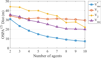
Figure 4: Tracking performance of multi-objective planning with $V_{mo}$ versus baseline methods in $100$ Monte Carlo runs as $|\mathcal{N}|$ increases from $2$ to $10$. $V_{mo}^{*}$ represents the optimal performance under ideal conditions where measurement origins are known.

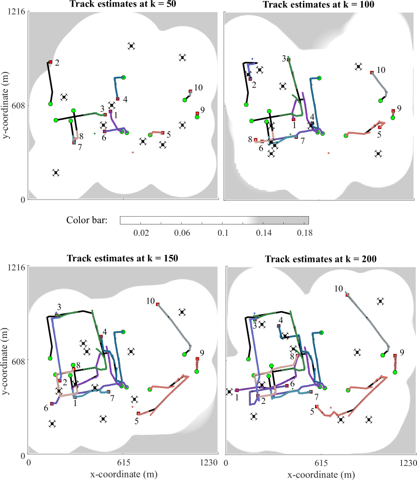
Figure 5: A sample run for multi-objective planning with $V_{mo}$. Background: grid occupancy probability. Foreground: estimated and true positions of $10$ taxis. Black lines show the ground truth trajectories, while the coloured dots denote the estimated positions. Circles ($\bigcirc$) and squares ($\Box$) mark taxi start/stop points, with different colours representing different taxi identities. The drone symbol indicates the positions of the 10 UAVs.

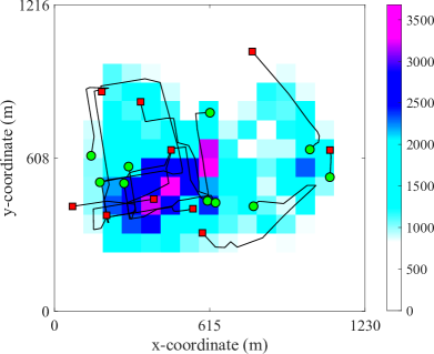
Figure 6: Heatmap ($16\times 16$ grids) showing the positions of $10$ UAVs and taxi trajectories in multi-objective planning with $V_{mo}$, averaged over $100$ MC runs. Circles ($\bigcirc$) and squares ($\Box$) indicate taxi start/stop positions. The colour legend represents UAV position frequency.

IV-B Results and Discussions

We first examine how the performance varies when the number of agents increases, specifically, for the following three planning strategies: (i) tracking only objective function $V_{1}$ (conventional approach); (ii) discovering only objective function $V_{2}$ (a special case of our approach); and (iii) multi-objective value function $V_{mo}$ that optimises trade-offs between tracking and discovering tasks (our approach). Note that, the value function $V_{1}$ is a conventional information-based method used in several previous works [7, 37, 38, 39, 40, 41], and hence, considered as a baseline for comparisons. Additionally, we also benchmark the planning algorithms against the ideal case when data association is known [24], i.e., the best possible tracking performance.

Fig. 4 shows the OSPA⁽²⁾ tracking error, over 100 Monte Carlo (MC) runs, for $10$ taxis in the CRAWDAD taxi dataset when the number of agents is increased from $2$ to $10$. On the one hand, when the number of agents is large (more than four), our proposed (multi-objective planning with) $V_{mo}$ constantly outperforms (single-objective planning with) $V_{1}$ and $V_{2}$, since there are enough agents to perform both tracking and discovering tasks simultaneously. On the other hand, when the number of agents is small (less than four), $V_{mo}$ achieves a similar accuracy as $V_{1}$ since there are not enough agents to cover the area, the multi-agent focused on tracking instead of exploring. As expected, $V_{1}$ does not improve tracking performance when the number of agents increases since it only focuses on tracking detected objects and misses objects outside of the team’s FoVs. Overall, multi-objective planning with $V_{mo}$ outperforms single-objective planning that either focuses on tracking, i.e., $V_{1}$, or discovering, i.e., $V_{2}$.

Further results for the 10-agent case demonstrate the effectiveness of multi-objective planning. Fig. 5 depicts the estimated versus true trajectories of the $10$ taxis (from the CRAWDAD taxi dataset), and the occupancy probability, at various times, for a particular run of the proposed (multi-objective planning with) $V_{mo}$. The results demonstrate the correct search and tracking of all taxis. The heat map over $100$ MC runs in Fig. 6, indicates that the $10$ agents concentrate on the western region of the search area where there are more taxis around, while also slightly covering the eastern region to successfully track the remaining taxis. It is expected that as time increases, the agents start to spread out from the centre to cover more areas for better discovery and tracking.

The mean and standard deviation (over $100$ MC runs) of the OSPA⁽²⁾ and cardinality errors for the different planning methods in Fig. 7, shows that the proposed $V_{mo}$ consistently outperforms $V_{1}$ (tracking-only) or $V_{2}$ (discovering-only) in terms of the overall tracking performance (i.e., OSPA⁽²⁾ Dist). Further, for localisation (i.e., OSPA⁽²⁾ Loc), the performance of $V_{mo}$ approaches that of the ideal case $V_{mo}^{*}$. We observe that most of the planning methods (in the experiment) can correctly estimate the number of taxis (i.e., Cardinality), except $V_{1}$, which only focuses on tracking and does not explore the areas outside the team’s FoVs. In terms of OSPA⁽²⁾ Card, since the cardinality is estimated correctly, most OSPA⁽²⁾ Card errors come from the track label switching and track fragmentation, which is expected given the limited FoVs, and the motion model mismatch between the CT model and the taxi’s occasional turns.

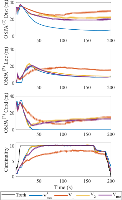
Figure 7: Overall tracking performance ($\mu\pm 0.2\sigma$) of the 10 agents versus time, over $100$ MC runs, for different planning methods.

V Conclusion

We have developed a multi-objective planning method for a limited-FoV multi-agent team to discover and track multiple mobile objects with unknown data association. The problem is formulated as a multi-agent POMDP with the multi-object filtering density as the information state. An entropy-based multi-objective value function is developed and shown to be monotone and submodular, thereby enabling low-cost implementation via greedy search with a tight optimality bound. A series of experiments on a real-world taxi dataset confirm our method’s capability and efficiency. It also validates the robustness of our proposed multi-objective formulation, wherein its overall performance shows a decreasing trend over time similar to that of the best possible performance. So far, we have considered a centralised architecture for multi-agent planning where scalability can be a limitation. A scalable approach should be a distributed POMDP for MOT, where each agent runs its local filter to track multi-objects and coordinates with other agents to achieve a global objective. However, planning for multi-agents to reach a global goal under a distributed POMDP framework is an NEXP-complete problem [2].

VI

VI-A Analytical Form of Tracking Value Function

To prove Proposition 1, we first require the three following Lemmas.

Lemma 1

For $f:\mathcal{F}(\mathbb{L})\rightarrow\mathbb{R}$, and $g:\mathbb{L}\rightarrow\mathbb{R}$,:

$$\sum_{L\subseteq\mathbb{L}}f(L)\sum_{\ell\in L}g(\ell)=\sum_{\ell\in\mathbb{L}}g(\ell)\sum_{L\subseteq\mathbb{L}\setminus\{\ell\}}f(L\cup\{\ell\})$$ (29)

Proof: This result was first presented in [54], but with an incomplete proof. We provide a complete proof via induction. It is trivial to confirm that (29) holds for $\mathbb{L}=\emptyset$ and $\mathbb{L}=\{\ell\}$. Suppose (29) holds for $\mathbb{L}=\{\ell_{1},\dots,\ell_{n}\}$. It remains to show that (29) also holds for $\mathbb{L}\cup\{\hat{\ell}\}$, i.e., $\displaystyle\!\!\!\!\!\!\sum_{L\subseteq\mathbb{L}\cup\hat{\ell}}f(L)\sum_{\ell\in L}g(\ell)$ $\displaystyle=\sum_{\ell\in\mathbb{L}\cup\hat{\ell}}g(\ell)\sum_{L\subseteq\mathbb{L}\cup\hat{\ell}\setminus\{\ell\}}f(L\cup\{\ell\}).$ (30)

Note that for any function $f:\mathcal{F}(\mathbb{L})\rightarrow\mathbb{R}$, $\displaystyle\sum_{L\subseteq\mathbb{L}\cup\hat{\ell}}f(L)=\sum_{L\subseteq\mathbb{L}}f(L)+\sum_{L\subseteq\mathbb{L}}f(L\cup\{\hat{\ell}\})$ (31) since $\mathcal{F}(\mathbb{L}\cup\hat{\ell})=\mathcal{F}(\mathbb{L})\cup\{(L\cup\{\widehat{\ell}\}):L\in\mathcal{F}(\mathbb{L})\}$ where $\mathcal{F}(\cdot)$ denotes the class of finite subsets. Hence, $\displaystyle\sum_{L\subseteq\mathbb{L}\cup\hat{\ell}}f(L)\sum_{\ell\in L}g(\ell)$ $\displaystyle=$ $\displaystyle\sum_{L\subseteq\mathbb{L}}f(L)\sum_{\ell\in L}g(\ell)+\sum_{L\subseteq\mathbb{L}}f(L\cup\{\hat{\ell}\})\sum_{\ell\in L\cup\{\hat{\ell}\}}g(\ell)$ (32)

Substituting (29) into (32), and noting that $\sum_{\ell\in L\cup\{\hat{\ell}\}}g(\ell)=\sum_{\ell\in L}g(\ell)+g(\hat{\ell})$, we have: $\displaystyle\sum_{L\subseteq\mathbb{L}\cup\hat{\ell}}f(L)\sum_{\ell\in L}g(\ell)$ $\displaystyle=$ $\displaystyle\sum_{\ell\in\mathbb{L}}g(\ell)\sum_{L\subseteq\mathbb{L}\setminus\{\ell\}}f(L\cup\{\ell\})+\sum_{L\subseteq\mathbb{L}}f(L\cup\{\hat{\ell}\})\sum_{\ell\in L}g(\ell)$ $\displaystyle+\sum_{L\subseteq\mathbb{L}}f(L\cup\{\hat{\ell}\})g(\hat{\ell})$ $\displaystyle=$ $\displaystyle\sum_{\ell\in\mathbb{L}}g(\ell)\sum_{L\subseteq\mathbb{L}\setminus\{\ell\}}f(L\cup\{\ell\})$ $\displaystyle+\sum_{\ell\in\mathbb{L}}g(\ell)\sum_{L\subseteq\mathbb{L}\setminus\{\ell\}}f(L\cup\{\hat{\ell}\}\cup\{\ell\})+g(\hat{\ell})\sum_{L\subseteq\mathbb{L}}f(L\cup\{\hat{\ell}\})$ $\displaystyle=$ $\displaystyle\sum_{\ell\in\mathbb{L}}g(\ell)\sum_{L\subseteq\mathbb{L}\cup\hat{\ell}\setminus\{\ell\}}f(L\cup\{\ell\})+g(\hat{\ell})\sum_{L\subseteq\mathbb{L}}f(L\cup\{\hat{\ell}\})$ $\displaystyle=$ $\displaystyle\sum_{\ell\in\mathbb{L}\cup\hat{\ell}}g(\ell)\sum_{L\subseteq\mathbb{L}\cup\hat{\ell}\setminus\{\ell\}}f(L\cup\{\ell\})\quad\Box.$

Lemma 2

For $f:\mathcal{F}(\mathbb{L})\rightarrow\mathbb{R}$, and $g:\mathbb{L}\rightarrow\mathbb{R}$, we have:

$$\sum_{L\subseteq\mathbb{L}}f(L)\sum_{\ell\in\mathbb{L}\setminus L}g(\ell)=\sum_{\ell\in\mathbb{L}}g(\ell)\sum_{L\subseteq\mathbb{L}\setminus\{\ell\}}f(L).$$ (33)

Proof: We prove this Lemma via induction. It is clear that (33) holds for $\mathbb{L}=\emptyset$ and $\mathbb{L}=\{\ell\}$. Now, assuming (33) for $\mathbb{L}=\{\ell_{1},\dots,\ell_{n}\}$, we demonstrate its validity for $\mathbb{L}\cup{\hat{\ell}}$, i.e.,:

$$\sum_{L\subseteq\mathbb{L}\cup\hat{\ell}}f(L)\sum_{\ell\in\mathbb{L}\cup\hat{\ell}\setminus L}g(\ell) =\sum_{\ell\in\mathbb{L}\cup\hat{\ell}}g(\ell)\sum_{L\subseteq\mathbb{L}\cup\hat{\ell}\setminus\{\ell\}}f(L).$$ (34)

Using (31) and noting that $\sum_{\ell\in\mathbb{L}\cup\{\hat{\ell}\}\setminus L}g(\ell)$ $=\sum_{\ell\in\mathbb{L}\setminus L}g(\ell)$ $+$ $g(\hat{\ell})$, we have:

$$\sum_{L\subseteq\mathbb{L}\cup\hat{\ell}}f(L)\sum_{\ell\in\mathbb{L}\cup\hat{\ell}\setminus L}g(\ell)$$

$$= \sum_{L\subseteq\mathbb{L}}f(L)\sum_{\ell\in\mathbb{L}\cup\hat{\ell}\setminus L}g(\ell)+\sum_{L\subseteq\mathbb{L}}f(L\cup\hat{\ell})\sum_{\ell\in\mathbb{L}\setminus L}g(\ell)$$

$$= \sum_{L\subseteq\mathbb{L}}f(L)\sum_{\ell\in\mathbb{L}\setminus L}g(\ell)+\sum_{L\subseteq\mathbb{L}}f(L)g(\hat{\ell})+\sum_{L\subseteq\mathbb{L}}f(L\cup\hat{\ell})\sum_{\ell\in\mathbb{L}\setminus L}g(\ell).$$ (35)

Substituting (33) into (35), we have:

$$\sum_{L\subseteq\mathbb{L}\cup\hat{\ell}}f(L)\sum_{\ell\in\mathbb{L}\cup\hat{\ell}\setminus L}g(\ell)$$

$$= \sum_{\ell\in\mathbb{L}}g(\ell)\sum_{L\subseteq\mathbb{L}\setminus\{\ell\}}f(L)+g(\hat{\ell})\sum_{L\subseteq\mathbb{L}}f(L)+\sum_{\ell\in\mathbb{L}}g(\ell)\sum_{L\subseteq\mathbb{L}\setminus\{\ell\}}f(L\cup\hat{\ell})$$

$$= \sum_{\ell\in\mathbb{L}}g(\ell)\sum_{L\subseteq\mathbb{L}\cup\hat{\ell}\setminus\{\ell\}}f(L)+g(\hat{\ell})\sum_{L\subseteq\mathbb{L}\cup\hat{\ell}\setminus\{\ell\}}f(L)$$

$$= \sum_{\ell\in\mathbb{L}\cup\hat{\ell}}g(\ell)\sum_{L\subseteq\mathbb{L}\cup\hat{\ell}\setminus\{\ell\}}f(L)\quad\Box.$$

Lemma 3

For $f:\mathcal{F}(\mathbb{L})\rightarrow\mathbb{R}$, $p:\mathbb{X}\times\mathbb{L}\rightarrow\mathbb{R}$, $q:\mathbb{X}\times\mathbb{L}\rightarrow\mathbb{R}$ with $q$ is a unitless function, we have:

$$\int\Delta(\boldsymbol{X})f(\mathcal{L}(\boldsymbol{X}))p^{\boldsymbol{X}}\ln q^{\boldsymbol{X}}\delta\boldsymbol{X}=\sum_{L\subseteq\mathbb{L}}f(L)\left\langle p\right\rangle^{L}\sum_{\ell\in L}\frac{\left\langle p\ln q\right\rangle(\ell)}{\left\langle p\right\rangle(\ell)}.$$

Proof: We first note that

$$I \triangleq\int\prod_{j=1}^{i}p(x_{j},\ell_{j})\ln\left(\prod_{n=1}^{i}q(x_{n},\ell_{n})\right)dx_{1:i}$$

$$=\int\prod_{j=1}^{i}p(x_{j},\ell_{j})\sum_{n=1}^{i}\ln q(x_{n},\ell_{n})dx_{1:i}$$

$$=\sum_{n=1}^{i}\int p(x,\ell_{n})\ln q(x,\ell_{n})dx\!\!\prod_{j\in\{1,\dots,i\}\setminus\{n\}}\!\!\int p(x,\ell_{j})dx$$

$$=\sum_{\ell\in\{\ell_{1:i}\}}\left\langle p\ln q\right\rangle(\ell)\left\langle p\right\rangle^{\{\ell_{1:i}\}-\{\ell\}}.~{}$$ (36)

Now

$$\int\Delta(\boldsymbol{X})f(\mathcal{L}(\boldsymbol{X}))p^{\boldsymbol{X}}\ln q^{\boldsymbol{X}}\delta\boldsymbol{X}$$

$$=f(\emptyset)p^{\emptyset}\ln q^{\emptyset}+\sum_{i=1}^{\infty}\frac{1}{i!}\sum_{\ell_{1:i}}\delta_{i}[|\{\ell_{1:i}\}|]f(\{\ell_{1},\dots,\ell_{i}\})\times I,$$

$$=\sum_{i=1}^{\infty}\frac{1}{i!}\sum_{\ell_{1:i}}\delta_{i}[|\{\ell_{1:i}\}|]f(\{\ell_{1},\dots,\ell_{i}\})\times I,$$ (37)

$$=\sum_{i=1}^{\infty}\frac{1}{i!}i!\sum_{L:|L|=i}f(L)\left[\sum_{\ell\in L}\left\langle p\right\rangle^{L-\{\ell\}}\left\langle p\ln q\right\rangle(\ell)\right]$$ (38)

$$=\sum_{L\subseteq\mathbb{L}}f(L)\left\langle p\right\rangle^{L}\sum_{\ell\in L}\frac{\left\langle p\ln q\right\rangle(\ell)}{\left\langle p\right\rangle(\ell)}$$ (39)

where (38) follows by substituting (36) into (37), and the last step follows from Lemma 12 in [32], and noting that

$$f(\emptyset)\left\langle p\right\rangle^{\emptyset}\sum_{\ell\in\emptyset}\frac{\left\langle p\ln q\right\rangle(\ell)}{\left\langle p\right\rangle(\ell)}=0~{}~{}~{}\Box.\hskip 71.13188pt$$ (40)

Proof of Proposition 1: For the LMB density, we have $\boldsymbol{\pi}(\boldsymbol{X})=\Delta(\boldsymbol{X})\tilde{r}^{\mathbb{L}\setminus\mathcal{L}(\boldsymbol{X})}r^{\mathcal{L}(\boldsymbol{X})}p^{\boldsymbol{X}}$; hence:

$$- h(\boldsymbol{X})=\int\boldsymbol{\pi}(\boldsymbol{X})\ln\big{(}K^{|\boldsymbol{X}|}\boldsymbol{\pi}(\boldsymbol{X})\big{)}\delta\boldsymbol{X}$$

$$= \int\Delta(\boldsymbol{X})\tilde{r}^{\mathbb{L}\setminus\mathcal{L}(\boldsymbol{X})}r^{\mathcal{L}(\boldsymbol{X})}p^{\boldsymbol{X}}\ln\big{[}\Delta(\boldsymbol{X})\tilde{r}^{\mathbb{L}\setminus\mathcal{L}(\boldsymbol{X})}r^{\mathcal{L}(\boldsymbol{X})}p^{\boldsymbol{X}}K^{|\boldsymbol{X}|}\big{]}\delta\boldsymbol{X}$$

$$= \int\Delta(\boldsymbol{X})\tilde{r}^{\mathbb{L}\setminus\mathcal{L}(\boldsymbol{X})}r^{\mathcal{L}(\boldsymbol{X})}p^{\boldsymbol{X}}\ln\big{[}\tilde{r}^{\mathbb{L}\setminus\mathcal{L}(\boldsymbol{X})}r^{\mathcal{L}(\boldsymbol{X})}\big{]}\delta\boldsymbol{X}$$

$$+\int\Delta(\boldsymbol{X})\tilde{r}^{\mathbb{L}\setminus\mathcal{L}(\boldsymbol{X})}r^{\mathcal{L}(\boldsymbol{X})}p^{\boldsymbol{X}}\ln\big{[}p^{\boldsymbol{X}}K^{|\boldsymbol{X}|}\big{]}\delta\boldsymbol{X}.$$ (41)

The first term on the right-hand side (RHS) of (41) is:

$$\int\Delta(\boldsymbol{X})\tilde{r}^{\mathbb{L}\setminus\mathcal{L}(\boldsymbol{X})}r^{\mathcal{L}(\boldsymbol{X})}p^{\boldsymbol{X}}\ln\big{[}\tilde{r}^{\mathbb{L}\setminus\mathcal{L}(\boldsymbol{X})}r^{\mathcal{L}(\boldsymbol{X})}\big{]}\delta\boldsymbol{X}$$ (42)

$$= \sum_{L\subseteq\mathbb{L}}\tilde{r}^{\mathbb{L}\setminus L}r^{L}\ln\big{[}\tilde{r}^{\mathbb{L}\setminus L}r^{L}\big{]}\bigg{[}\int p(x,\cdot)dx\bigg{]}^{L}$$ (43)

$$= \sum_{L\subseteq\mathbb{L}}\tilde{r}^{\mathbb{L}\setminus L}r^{L}\sum_{\ell\in\mathbb{L}\setminus L}\ln\tilde{r}^{(\ell)}+\sum_{L\subseteq\mathbb{L}}\tilde{r}^{\mathbb{L}\setminus L}r^{L}\sum_{\ell\in L}\ln r^{(\ell)}$$ (44)

$$= \sum_{\ell\in\mathbb{L}}\ln\tilde{r}^{(\ell)}\sum_{L\subseteq\mathbb{L}\setminus\{\ell\}}\tilde{r}^{\mathbb{L}\setminus L}r^{L}$$

$$\quad+\sum_{\ell\in\mathbb{L}}\ln r^{(\ell)}\sum_{L\subseteq\mathbb{L}\setminus\{\ell\}}\tilde{r}^{\mathbb{L}\setminus(L\cup\{\ell\})}r^{L\cup\{\ell\}}$$ (45)

$$= \sum_{\ell\in\mathbb{L}}\bigg{[}\tilde{r}^{(\ell)}\ln\tilde{r}^{(\ell)}\sum_{L\subseteq\mathbb{L}\setminus\{\ell\}}\tilde{r}^{(\mathbb{L}\setminus\{\ell\})\setminus L}r^{L}$$

$$\quad\quad\quad+r^{(\ell)}\ln r^{(\ell)}\sum_{L\subseteq\mathbb{L}\setminus\{\ell\}}\tilde{r}^{(\mathbb{L}\setminus\{\ell\})\setminus L}r^{L}\bigg{]}$$ (46)

$$= \sum_{\ell\in\mathbb{L}}\left[r^{(\ell)}\ln r^{(\ell)}+\tilde{r}^{(\ell)}\ln\tilde{r}^{(\ell)}\right].$$ (47)

Here, (43) follows from Lemma 3 in [32]; (44) follows from $\int p(x,\cdot)dx=1$; each term in (45) follows from Lemma 2 and Lemma 1, respectively; while (47) follows from the Binomial Theorem, i.e., $\sum_{L\subseteq\mathbb{L}}f^{\mathbb{L}\setminus L}g^{L}=(f+g)^{\mathbb{L}}$. Hence, $\sum_{L\subseteq\mathbb{L}\setminus\{\ell\}}\tilde{r}^{(\mathbb{L}\setminus\{\ell\})\setminus L}r^{L}=(\tilde{r}+r)^{\mathbb{L}\setminus\{\ell\}}=1$.

The second term of the RHS of (41) is:

$$\int\Delta(\boldsymbol{X})\tilde{r}^{\mathbb{L}\setminus\mathcal{L}(\boldsymbol{X})}r^{\mathcal{L}(\boldsymbol{X})}p^{\boldsymbol{X}}\ln\big{[}p^{\boldsymbol{X}}K^{|\boldsymbol{X}|}\big{]}\delta\boldsymbol{X}$$ (48)

$$= \sum_{L\subseteq\mathbb{L}}\tilde{r}^{\mathbb{L}\setminus L}r^{L}\sum_{\ell\in L}\left\langle p^{(\ell)}\ln(Kp^{(\ell)})\right\rangle$$ (49)

$$= \sum_{\ell\in\mathbb{L}}\left\langle p^{(\ell)}\ln(Kp^{(\ell)})\right\rangle\sum_{L\subseteq\mathbb{L}\setminus\{\ell\}}\tilde{r}^{\mathbb{L}\setminus(L\cup\{\ell\})}r^{L\cup\{\ell\}}$$ (50)

$$= \sum_{\ell\in\mathbb{L}}r^{(\ell)}\left\langle p^{(\ell)}\ln(Kp^{(\ell)})\right\rangle\sum_{L\subseteq\mathbb{L}\setminus\{\ell\}}\tilde{r}^{(\mathbb{L}\setminus\{\ell\})\setminus L}r^{L}$$ (51)

$$= \sum_{\ell\in\mathbb{L}}r^{(\ell)}\left\langle p^{(\ell)}\ln(Kp^{(\ell)})\right\rangle.$$ (52)

Here, (49) follows from Lemma 3; (50) follows from Lemma 1; while (52) follows from the Binomial Theorem, i.e., $\sum_{L\subseteq\mathbb{L}\setminus\{\ell\}}\tilde{r}^{(\mathbb{L}\setminus\{\ell\})\setminus L}r^{L}=(\tilde{r}+r)^{\mathbb{L}\setminus\{\ell\}}=1$.

Substituting (47) and (52) into (41), we have:

$$h(\boldsymbol{X})=-\sum_{\ell\in\mathbb{L}}\left[r^{(\ell)}\ln r^{(\ell)}+\tilde{r}^{(\ell)}\ln\tilde{r}^{(\ell)}+r^{(\ell)}\left\langle p^{(\ell)}\ln(Kp^{(\ell)})\right\rangle\right]\Box.$$

VI-B Analytical Form of Discovery Value Function

Proof of Proposition 2: The predicted occupancy probability in (18) is straight forward. To establish (19), note that

$$\textrm{Pr}(O_{j+1}^{(i)}=1,Y_{a_{j},j+1}^{(i)}=1)\! =\! \omega_{j+1}^{(i)}(a_{j-1})Q_{D,+}^{(i)}(a_{j}),$$

$$\textrm{Pr}(O_{j+1}^{(i)}=0,Y_{a_{j},j+1}^{(i)}=1)\! =\! 1-\omega_{j+1}^{(i)}(a_{j-1}).$$

Therefore, $\textrm{Pr}(Y_{a_{j},j+1}^{(i)}=1)=1-\omega{}_{j+1}^{(i)}(a_{j-1})+$ $\omega_{j+1}^{(i)}(a_{j-1})Q_{D,+}^{(i)}(a_{j})$, and using Bayes’ rule yields (19).

Note that if $\varkappa^{(i)}$ generates measurements (i.e., $Y_{a,j}^{(i)}=0$), then it is occupied (i.e., $O_{j}^{(i)}=1$), which means

$$\textrm{Pr}(O_{j}^{(i)}=0|Y_{a,j}^{(i)}=0)\! =\! 0.$$

$$\textrm{Pr}(O_{j}^{(i)}=1|Y_{a,j}^{(i)}=0)\! =\! 1.$$

Hence, $h(O_{j}^{(i)}|Y_{a,j}^{(i)}=0)=0\ln 0+1\ln 1=0$, and

$$h(O_{j}^{(i)}|Y_{a,j}^{(i)}) =\textrm{Pr}(Y_{a,j}^{(i)}=1)h(O_{j}^{(i)}|Y_{a,j}^{(i)}=1).$$ (53)

Substituting for $\textrm{Pr}(O_{j}^{(i)}=1|Y_{a,j}^{(i)}=1)$ and $\textrm{Pr}(Y_{a,j}^{(i)}=1)$ yields (17) $\Box.$

VI-C Monotone Submodularity

To prove Proposition 3, we first require the following result.

Lemma 4

$\forall\boldsymbol{R}\subseteq\boldsymbol{Z}\in\boldsymbol{\mathbb{\mathcal{Z}}}$ and $\forall\boldsymbol{Y}\in\boldsymbol{\mathcal{Z}}\setminus\boldsymbol{Z}$:

$$I(\boldsymbol{X};\boldsymbol{Z},\boldsymbol{Y})-I(\boldsymbol{X};\boldsymbol{Z}) \leq I(\boldsymbol{X};\boldsymbol{R},\boldsymbol{Y})-I(\boldsymbol{X};\boldsymbol{R}).$$

Proof : Since $\boldsymbol{R}\subseteq\boldsymbol{Z}\in\boldsymbol{\mathbb{\mathcal{Z}}}$, using the mutual information inequalities [6, p.50], we have:

$$I(\boldsymbol{Z};\boldsymbol{Y})\geq I(\boldsymbol{R};\boldsymbol{Y})$$

$$\Leftrightarrow h(\boldsymbol{Y})-h(\boldsymbol{Y}|\boldsymbol{Z})\geq h(\boldsymbol{Y})-h(\boldsymbol{Y}|\boldsymbol{R})$$

$$\Leftrightarrow h(\boldsymbol{Y}|\boldsymbol{R})\geq h(\boldsymbol{Y}|\boldsymbol{Z}),$$

$$\Leftrightarrow h(\boldsymbol{R},\boldsymbol{Y})-h(\boldsymbol{R})\geq h(\boldsymbol{Z},\boldsymbol{Y})-h(\boldsymbol{Z}).$$ (55)

Further, nothing that $I(\boldsymbol{Z};\boldsymbol{Y}|\boldsymbol{X})=I(\boldsymbol{R};\boldsymbol{Y}|\boldsymbol{X})=0$ because $\boldsymbol{Y}$ is independent of $\boldsymbol{R}$ and $\boldsymbol{Z}$, given $\boldsymbol{X}$, we have,

$$h(\boldsymbol{Y}|\boldsymbol{X}) =h(\boldsymbol{Y}|\boldsymbol{X},\boldsymbol{Z})+I(\boldsymbol{Z};\boldsymbol{Y}|\boldsymbol{X})=h(\boldsymbol{Y}|\boldsymbol{X},\boldsymbol{Z})$$

$$=h(\boldsymbol{X},\boldsymbol{Z},\boldsymbol{Y})-h(\boldsymbol{X},\boldsymbol{Z}),$$

$$=h(\boldsymbol{Y}|\boldsymbol{X},\boldsymbol{R})+I(\boldsymbol{R};\boldsymbol{Y}|\boldsymbol{X})$$

$$=h(\boldsymbol{X},\boldsymbol{R},\boldsymbol{Y})-h(\boldsymbol{X},\boldsymbol{R}).$$

and hence,

$$h(\boldsymbol{X},\boldsymbol{Z},\boldsymbol{Y})-h(\boldsymbol{X},\boldsymbol{Z})=h(\boldsymbol{X},\boldsymbol{R},\boldsymbol{Y})-h(\boldsymbol{X},\boldsymbol{R}).$$ (56)

Subtracting (55) from (56), we have:

$$\!\!\!\!\!\!\!\!\![h(\boldsymbol{X},\boldsymbol{Z},\boldsymbol{Y})-h(\boldsymbol{X},\boldsymbol{Z})]-[h(\boldsymbol{Z},\boldsymbol{Y})-h(\boldsymbol{Z})]$$

$$\geq[h(\boldsymbol{X},\boldsymbol{R},\boldsymbol{Y})-h(\boldsymbol{X},\boldsymbol{R})]-[h(\boldsymbol{R},\boldsymbol{Y})-h(\boldsymbol{R})]$$

Note from the differential entropy chain rules [6, p.253] that $h(\boldsymbol{X}|\boldsymbol{Z},\boldsymbol{Y})=h(\boldsymbol{X},\boldsymbol{Z},\boldsymbol{Y})-h(\boldsymbol{Z},\boldsymbol{Y})$ and $h(\boldsymbol{X}|\boldsymbol{Z})=h(\boldsymbol{X},\boldsymbol{Z})-h(\boldsymbol{Z})$. Substituting these into the above gives

$$h(\boldsymbol{X}|\boldsymbol{Z},\boldsymbol{Y})-h(\boldsymbol{X}|\boldsymbol{Z})\geq h(\boldsymbol{X}|\boldsymbol{R},\boldsymbol{Y})-h(\boldsymbol{X}|\boldsymbol{R})$$

$$\Leftrightarrow [h(\boldsymbol{X})-h(\boldsymbol{X}|\boldsymbol{Z},\boldsymbol{Y})]-[h(\boldsymbol{X})-h(\boldsymbol{X}|\boldsymbol{Z})]$$

$$\leq[h(\boldsymbol{X})-h(\boldsymbol{X}|\boldsymbol{R},\boldsymbol{Y}]-[h(\boldsymbol{X})-h(\boldsymbol{X}|\boldsymbol{R})],$$

$$\Leftrightarrow I(\boldsymbol{X};\boldsymbol{Z},\boldsymbol{Y})-I(\boldsymbol{X};\boldsymbol{Z})\leq I(\boldsymbol{X};\boldsymbol{R},\boldsymbol{Y})-I(\boldsymbol{X};\boldsymbol{R}).\mathbf{\Box.}$$

Proof of Proposition 3: Denote $\boldsymbol{\breve{\pi}}(\boldsymbol{Z}_{1}\cup\boldsymbol{Z}_{2})\equiv\boldsymbol{\pi}(\boldsymbol{Z}_{1},\boldsymbol{Z}_{2})$, then according to (3.53) and (25.36) in [20]: $\int\boldsymbol{\breve{\pi}}(\boldsymbol{Z}_{1}\cup\boldsymbol{Z}_{2})\delta(\boldsymbol{Z}_{1}\cup\boldsymbol{Z}_{2})=\int{\boldsymbol{\pi}(\boldsymbol{Z}_{1},\boldsymbol{Z}_{2})}\delta\boldsymbol{Z}_{1}\delta\boldsymbol{Z}_{2}$. Further, noting that

$$I(\boldsymbol{X};\boldsymbol{Z})=\int\boldsymbol{\pi}(\boldsymbol{X,Z})\ln\left(\dfrac{\boldsymbol{\pi}(\boldsymbol{X,Z})}{\boldsymbol{\pi}(\boldsymbol{X})\boldsymbol{\pi}(\boldsymbol{Z})}\right)\delta\boldsymbol{X}\delta\boldsymbol{Z}$$

$$I(\boldsymbol{X};\boldsymbol{Z_{1},Z_{2}})=\int\boldsymbol{\pi}(\boldsymbol{X,Z_{1},Z_{2}})\ln\left(\dfrac{\boldsymbol{\pi}(\boldsymbol{X,Z_{1},Z_{2}})}{\boldsymbol{\pi}(\boldsymbol{X})\boldsymbol{\pi}(\boldsymbol{Z_{1},Z_{2}})}\right)\delta\boldsymbol{X}\delta\boldsymbol{Z_{1}}\delta\boldsymbol{Z_{2}}.$$

we have $I(\boldsymbol{X};\boldsymbol{Z}_{1}\cup\boldsymbol{Z}_{2})=I(\boldsymbol{X};\boldsymbol{Z}_{1},\boldsymbol{Z}_{2})$.

Due to the mutual exclusiveness of the multi-object measurements between the agents, and the independence of an agent’s measurement from the other agent’s actions, $\boldsymbol{Z}_{\boldsymbol{A},j}=\uplus_{\boldsymbol{a}\in\boldsymbol{A}}\boldsymbol{\boldsymbol{Z}}_{\boldsymbol{a},j}$, where $\boldsymbol{\boldsymbol{Z}}_{(a^{(m)},m),j}$ is the measurement set received by agent $m$ at time $j$ after it has taken action $a^{(m)}$. Hence, for $\boldsymbol{A}\subseteq\boldsymbol{B}\subset\boldsymbol{\mathbb{A}}$, $\boldsymbol{a}\in\boldsymbol{\mathbb{A}}\setminus\boldsymbol{B}$, we have: $\boldsymbol{Z}_{\boldsymbol{A}}\subseteq\boldsymbol{Z}_{\boldsymbol{B}}$ and $\boldsymbol{Z}_{\boldsymbol{a}}\in\boldsymbol{\mathcal{Z}}\setminus\boldsymbol{Z}_{\boldsymbol{B}}$. Thus, it follows from Lemma 4 that

$$I(\boldsymbol{X};\boldsymbol{Z}_{\boldsymbol{B}},\boldsymbol{Z}_{\boldsymbol{a}})-I(\boldsymbol{X};\boldsymbol{Z}_{\boldsymbol{B}})\leq I(\boldsymbol{X};\boldsymbol{Z}_{\boldsymbol{A}},\boldsymbol{Z}_{\boldsymbol{a}})-I(\boldsymbol{X};\boldsymbol{Z}_{\boldsymbol{A}}),$$

which is equivalent to

$$I(\boldsymbol{X};\boldsymbol{Z}_{\boldsymbol{B}\cup\{\boldsymbol{a}\}})-I(\boldsymbol{X};\boldsymbol{Z}_{\boldsymbol{B}})\leq I(\boldsymbol{X};\boldsymbol{Z}_{\boldsymbol{A}\cup\{\boldsymbol{a}\}}-I(\boldsymbol{X};\boldsymbol{Z}_{\boldsymbol{A}}).$$

i.e., $I(\boldsymbol{X};\boldsymbol{Z}_{\boldsymbol{A}})$ is a submodular set function. Further, using the chain rule we have:

$$I(\boldsymbol{X};\boldsymbol{Z}_{\boldsymbol{A}},\boldsymbol{Z}_{\boldsymbol{a}})-I(\boldsymbol{X};\boldsymbol{Z}_{\boldsymbol{A}})=I(\boldsymbol{X};\boldsymbol{Z}_{\boldsymbol{A}}|\boldsymbol{Z}_{\boldsymbol{a}})\geq 0$$

i.e., $I(\boldsymbol{X};\boldsymbol{Z}_{\boldsymbol{A}})$ is a monotone submodular set function $\Box$.

Proof of Proposition 5: Let $\boldsymbol{Y}_{\boldsymbol{A}}^{(i)}=\uplus_{\boldsymbol{a}\in\boldsymbol{A}}\boldsymbol{Y}_{\boldsymbol{a}}^{(i)}$, where $\boldsymbol{Y}_{(a^{(m)},m)}^{(i)}=(Y_{(a^{(m)},m)}^{(i)},m)$, and $Y_{(a^{(m)},m)}^{(i)}$ is the binary measurement $\delta_{\emptyset}[\boldsymbol{Z}_{(a^{(m)},m)}(\varkappa^{(i)})]$ received by agent $m$ from cell $\varkappa^{(i)}$, after it has taken action $(a^{(m)},m)$. Note that the binary measurement $Y_{\boldsymbol{A}}^{(i)}=\delta_{\emptyset}[\boldsymbol{Z}_{\boldsymbol{A}}(\varkappa^{(i)})]$ received from cell $\varkappa^{(i)}$ can be written as $\prod_{\boldsymbol{a}\in\boldsymbol{A}}Y{}_{\boldsymbol{a}}^{(i)}$, due to the independence of the agent’s measurement from the other agent’s actions. We first show by induction that

$$h(O^{(i)}|\boldsymbol{Y}{}_{\boldsymbol{A}}^{(i)}) =h(O^{(i)}|Y_{\boldsymbol{A}}^{(i)})$$ (57)

It is trivial to confirm that (57) holds for $\{\boldsymbol{a}\}$. Suppose that (57) holds for a non-empty $\boldsymbol{A}$, then

$$h(O^{(i)}|\boldsymbol{Y}_{\boldsymbol{A}}^{(i)})=h(O^{(i)}|Y_{\boldsymbol{A}}^{(i)})=\textrm{Pr}(Y_{\boldsymbol{A}}^{(i)}=1)h(O^{(i)}|Y_{\boldsymbol{A}}^{(i)}=1).$$ (58)

Decomposing $\boldsymbol{Y}_{\boldsymbol{A}\cup\{\boldsymbol{a}\}}^{(i)}$, we have

$$h(O^{(i)}|\boldsymbol{Y}_{\boldsymbol{A}\cup\{\boldsymbol{a}\}}^{(i)})=h(O^{(i)}|\boldsymbol{Y}_{\boldsymbol{A}}^{(i)},\boldsymbol{Y}_{\boldsymbol{a}}^{(i)})$$

$$=\textrm{Pr}(\boldsymbol{Y}_{\boldsymbol{a}}^{(i)}=0)h(O^{(i)}|\boldsymbol{Y}_{\boldsymbol{A}}^{(i)},\boldsymbol{Y}_{\boldsymbol{a}}^{(i)}=0)$$

$$\quad\quad+\textrm{Pr}(\boldsymbol{Y}_{\boldsymbol{a}}^{(i)}=1)h(O^{(i)}|\boldsymbol{Y}_{\boldsymbol{A}}^{(i)},\boldsymbol{Y}_{\boldsymbol{a}}^{(i)}=1)$$ (59)

$$=\textrm{Pr}(\boldsymbol{Y}_{\boldsymbol{a}}^{(i)}=1)h(O^{(i)}|\boldsymbol{Y}_{\boldsymbol{A}}^{(i)},\boldsymbol{Y}_{\boldsymbol{a}}^{(i)}=1)$$ (60)

since $h(O^{(i)}|\boldsymbol{Y}_{\boldsymbol{A}}^{(i)},\boldsymbol{Y}_{\boldsymbol{a}}^{(i)}=0)=h(O^{(i)}|Y_{\boldsymbol{A}\cup\{\boldsymbol{a}\}}^{(i)}=0)=0$. Substitute (58) into (60), we have:

$$h(O^{(i)}|\boldsymbol{Y}_{\boldsymbol{A}\cup\{\boldsymbol{a}\}}^{(i)})$$

$$=\textrm{Pr}(\boldsymbol{Y}_{\boldsymbol{a}}^{(i)}=1)\textrm{Pr}(Y_{\boldsymbol{A}}^{(i)}=1)h(O^{(i)}|Y_{\boldsymbol{A}}^{(i)}=1,\boldsymbol{Y}_{\boldsymbol{a}}^{(i)}=1)$$

$$=\textrm{Pr}(Y_{\boldsymbol{A}\cup\{\boldsymbol{a}\}}^{(i)}=1)h(O^{(i)}|Y_{\boldsymbol{A}\cup\{\boldsymbol{a}\}}^{(i)}=1)$$

$$=h(O^{(i)}|Y_{\boldsymbol{A}\cup\{\boldsymbol{a}\}}^{(i)}).\quad\quad\quad$$

From Proposition 3, $-h(O^{(i)}|\boldsymbol{Y}_{\boldsymbol{A}}^{(i)})$, and hence $-h(O^{(i)}|Y_{\boldsymbol{A}}^{(i)})$, are monotone submodular. Consequently, it follows from [22, pp.272] that $V_{2}(\boldsymbol{A})$ is monotone submodular because it is a positive linear combination $-h(O^{(i)}|Y_{\boldsymbol{A}}^{(i)})$  $\Box$.