The fractal geometry of growth: fluctuation-dissipation theorem and hidden symmetry

Abstract

Growth in crystals can be usually described by field equations such as the Kardar-Parisi-Zhang (KPZ) equation. While the crystalline structure can be characterized by Euclidean geometry with its peculiar symmetries, the growth dynamics creates a fractal structure at the interface of a crystal and its growth medium, which in turn determines the growth. Recent work (The KPZ exponents for the 2+ 1 dimensions, MS Gomes-Filho, ALA Penna, FA Oliveira; Results in Physics, 104435 (2021)) associated the fractal dimension of the interface with the growth exponents for KPZ, and provides explicit values for them. In this work we discuss how the fluctuations and the responses to it are associated with this fractal geometry and the new hidden symmetry associated with the universality of the exponents.

I Introduction

Symmetry and spontaneous symmetry breaking are fundamental concepts to understanding nature, in particular to investigate the phases of matter. Since growth is one of the most ubiquitous phenomenon in nature, a question appears immediately “What are the symmetries associated with growth?” In order to address this question we shall look to the major growth field equations. Two basic equations are the Edwards Wilkinson (EW) Edwards and Wilkinson (1982):

$$\dfrac{\partial h(\vec{x},t)}{\partial t}=\nu\nabla^{2}h(\vec{x},t)+\xi(\vec{x},t),$$ (1)

and the Kardar-Parisi-Zhang equation Kardar et al. (1986):

$$\dfrac{\partial h(\vec{x},t)}{\partial t}=\nu\nabla^{2}h(\vec{x},t)+\dfrac{\lambda}{2}[\vec{\nabla}h(\vec{x},t)]^{2}+\xi(\vec{x},t),$$ (2)

where $h:\mathbb{R}^{d}\times\mathbb{R}^{+}\rightarrow\mathbb{R}$ denotes the interface heights at point $\vec{x}\in\mathbb{R}^{d}$ at the time $t\geqslant 0$. Since $h(\vec{x},t)$ displays different scale properties than those displayed by $\vec{x}$, we say that we have a $d+1$ dimensional space, in such way that the growth of a film will be in $2+1$ space dimensions. The parameters $\nu$ (surface tension) and $\lambda$ are related to the Laplacian smoothing and the tilt mechanism, respectively. The stochastic process is characterized by the zero mean white noise, $\xi(\vec{x},t)$, with:

$$\left\langle\xi(\vec{x},t)\xi(\vec{x}^{\prime},t^{\prime})\right\rangle=2D\delta^{(d)}(\vec{x}-\vec{x}^{\prime})\delta(t-t^{\prime}),$$ (3)

where $D$ is here the noise intensity. The above equation is sometimes called the Fluctuation-dissipation theorem (FDT). The EW equation were obtained Edwards and Wilkinson (1982); Barabási and Stanley (1995) considering the basic symmetries $\vec{x}\rightarrow\vec{x}+\vec{x}_{0}$, $\vec{x}\rightarrow-\vec{x}$, $t\rightarrow t+t_{0}$, $h\rightarrow h+h_{0}$ and $h\rightarrow-h$, i.e. independence of the frame of reference. Note that the symmetry $h\rightarrow-h$ is violated for KPZ due to the presence of the non-linear dependence on the local slope $[\vec{\nabla}h]^{2}$. The KPZ equation describes very well the dynamics of some atomistic models such as the etching model Mello et al. (2001); Reis (2005); Almeida et al. (2014); Rodrigues et al. (2014); Alves et al. (2016); Carrasco and Oliveira (2018), and the Single-Step (SS) model Krug et al. (1992); Krug (1997); Derrida and Lebowitz (1998); Meakin et al. (1986); Daryaei (2020) in the long wavelength limit. For atomistic models we define our Euclidean space as a $d$-dimensional hypercubic lattice within the region $\Omega\subset\mathbb{R}^{d}$, with volume $V=L^{d}$, where $L$ is the lateral side.

Two quantities play an important role in growth, the average height, $\langle h(t)\rangle$, and the standard deviation

$$w(L,t)=\left[\langle h^{2}(t)\rangle-\langle h(t)\rangle^{2}\right]^{1/2},$$ (4)

which is named as roughness or the surface width. Here the average is taken over the space. The roughness is a very important physical quantity, since many important phenomena have been associated with it Edwards and Wilkinson (1982); Kardar et al. (1986); Barabási and Stanley (1995); Mello et al. (2001); Reis (2005); Almeida et al. (2014); Rodrigues et al. (2014); Alves et al. (2016); Carrasco and Oliveira (2018); Krug et al. (1992); Krug (1997); Derrida and Lebowitz (1998); Meakin et al. (1986); Daryaei (2020); Hansen et al. (2000). For many growth processes, the roughness, $w(L,t)$, increases with time until reaches a saturated roughness $w_{s}$, i.e., $w(t\rightarrow\infty)=w_{s}$. We can summarize the time evolution of all regions as following Barabási and Stanley (1995):

$$w(L,t)=\begin{cases}ct^{\beta},&\text{ if~{}~{} }t<<t_{\times}\\ w_{s}\propto L^{\alpha},&\text{ if~{}~{} }t>>t_{\times},\\ \end{cases}$$ (5)

with $t_{\times}\propto L^{z}$. The dynamical exponents satisfy the general scaling relation:

$$z=\frac{\alpha}{\beta}.$$ (6)

The set of exponents $(\alpha,\beta,z)$ define the growth process, and its universality class Barabási and Stanley (1995). Since the universality class is associated with the symmetries, the breaking of the symmetry $h\rightarrow-h$ turns out the KPZ universality class different from that of EW. For example, for the KPZ universality class, the Galilean invariance Kardar et al. (1986):

$$\alpha+z=2,$$ (7)

is a signature of KPZ.

In this way, the KPZ equation, Eq. (2), is a general nonlinear stochastic differential equation, which can characterize the growth dynamics of many different systems Mello et al. (2001); Reis (2005); Almeida et al. (2014); Rodrigues et al. (2014); Alves et al. (2016); Carrasco and Oliveira (2018); Merikoski et al. (2003); Ódor et al. (2010); Takeuchi (2013); Almeida et al. (2017). As consequence most of these stochastic systems are interconnected. For instance, the SS model Krug et al. (1992); Krug (1997); Derrida and Lebowitz (1998); Meakin et al. (1986); Daryaei (2020), which is connected with the asymmetric simple exclusion process Derrida and Lebowitz (1998), the six-vertex model Meakin et al. (1986); Gwa and Spohn (1992); De Vega and Woynarovich (1985), and the kinetic Ising model Meakin et al. (1986); Plischke et al. (1987), all of them are of fundamental importance. It is noteworthy that quantum versions of the KPZ equation have been recently reported that are connected with a Coulomb gas Corwin et al. (2018), a quantum entanglement growth dynamics with random time and space Nahum et al. (2017), as well as in infinite temperature spin-spin correlation in the isotropic quantum Heisenberg spin-$1/2$ model Ljubotina et al. (2019); De Nardis et al. (2019).

Despite all effort, finding an analytical, or even a numerical solution, of the KPZ equation (2) is not an easy task Dasgupta et al. (1996, 1997); Torres and Buceta (2018); Wio et al. (2010, 2017); Rodríguez and Wio (2019) and we are still far from a satisfactory theory for the KPZ equation, which makes it one of the most difficult and exciting problems in modern mathematical physics Bertini and Giacomin (1997); Baik et al. (1999); Prähofer and Spohn (2000); Dotsenko (2010); Calabrese et al. (2010); Amir et al. (2011); Sasamoto and Spohn (2010); Le Doussal et al. (2016); Hairer (2013), and probably one of the most important problem in non equilibrium statistical physics. The outstanding works of Prähofer and Spohn Prähofer and Spohn (2000) and Johansson Johansson (2000) opened the possibility of an exact solution for the distributions of the heights fluctuations $f(h,t)$ in the KPZ equation for $1+1$ dimensions (for reviews see Calabrese et al. (2010); Amir et al. (2011); Sasamoto and Spohn (2010); Le Doussal et al. (2016); Hairer (2013); Johansson (2000) ).

In a recent work Gomes-Filho et al. (2021) the exponents were determined for $2+1$ dimensions using

$$\alpha=\begin{cases}1/2,&\text{ if~{}~{} }d=1\\ \frac{1}{d_{f}+1},&\text{ if~{}~{} }d\geqslant 2,\\ \end{cases}$$ (8)

where $d_{f}$ denote the fractal (Hausdorff) dimension of the interface, which has been proved to be as well associated with the global roughness exponent $\alpha$, and the well known result Barabási and Stanley (1995)

$$\alpha=2-d_{f},$$ (9)

for $d=1,2$. This yields for $2+1$ dimensions

$$z=d_{f}=\varphi,\hskip 19.91684pt\alpha=\frac{3-\sqrt{5}}{2},\hskip 19.91684pt\beta=\sqrt{5}-2,$$ (10)

where $\varphi=\frac{1+\sqrt{5}}{2}$ is the golden ratio.

In this work we discuss a fluctuation-dissipation theorem for growth in $d+1$ dimensions and the possible symmetries associated with the fractal geometry of growth.

II Fractality, symmetry and universality

Note that now we do not have just the triad $(\alpha,\beta,z)$ but the quaternary $(d_{f},\alpha,\beta,z)$, i.e. the fractal dimension and the exponents. They are completely connected, thus fractality, symmetry and universality are interconnected as well. Using the Eqs. (6), (7), (8) and (9) we can determine $(d_{f},\alpha,\beta,z)$. Therefore for $2+1$ dimensions, under any point of view, the exponents and fractal dimension have been determined. However, there are questions concerning the symmetries that we have not even touched. The first question is why Eq. (8) has a distinct behavior for $d=1$ and $d\neq 1$? The value $\alpha=1/2$ for $d=1$, i.e. $1+1$ dimensions, is known since the KPZ original work Kardar et al. (1986). It is a consequence of the validity of the FDT (3) for this dimension. Nonetheless, we have some new elements for $d>1$, the explicit appearance of this new non-Euclidean dimension requires a more detailed analysis of the involved symmetries.

III Fluctuations relations and fractal geometry

In order to understanding deeply the fluctuation-dissipation relation we have to go back to the works of Einstein, Smoluchowski and Langevin on the Brownian motion Brown (1828a, b); Einstein (1905, 1956); Langevin (1908); Vainstein et al. (2006); Gudowska-Nowak et al. (2017); Oliveira et al. (2019). Langevin proposed a Newton equation of motion for a particle moving in a fluid as Langevin (1908):

$$\frac{\mathrm{d}P(t)}{\mathrm{d}t}=-\gamma P(t)+f(t),$$ (11)

where $P$ is the particle momentum and $\gamma$ is the friction. The ingenious and elegant proposal was to modulate the complex interactions between particles, considering all interactions as two main forces: the first contribution represents a frictional force, $-\gamma P$, where the characteristic time scale is $\tau=\gamma^{-1}$ while the second contribution comes from a stochastic force, $f(t)$, with time scale $\Delta t\ll\tau$, which is related with the random collisions between the particle and the fluid molecules. The uncorrelated force $f(t)$ is given by

$$\langle f(t)f(t^{\prime})\rangle=2\gamma\langle P^{2}\rangle_{eq}\delta(t-t^{\prime}),$$ (12)

where $\langle P^{2}\rangle_{eq}=mk_{B}T$, where $k_{B}$ is the Boltzmann constant. Note that Eq. (12) was obtained by imposing that the mean square momentum reaches a fixed value given by the equipartition theorem, i.e. there is an energy conservation on the average, which means a time translation symmetry. Later on Onsager Onsager (1931) demonstrated that symmetries in the susceptibility (response functions) were associated with the crystal symmetry.

More recently, it was observed Gomes-Filho and Oliveira (2021) that even for $1+1$ dimensions in growth process Eq. (12) is not really a FDT, but a relation for the noise intensity, so the FDT relation was completed using the exact result of Krug et al. Krug et al. (1992); Krug (1997) for the saturated roughness:

$$w_{s}=\sqrt{\frac{D}{24\nu}L},$$ (13)

in $1+1$ dimensions. This shows that the saturation is an interplay between noise $D$, which increases the saturation, and the surface tension $\nu$, which opposes to the curvature, acting as a “friction” for the roughness. And therefore the FDT for growth can be written as Gomes-Filho and Oliveira (2021):

$$\left\langle\xi({x},t)\xi({x^{\prime}},t^{\prime})\right\rangle=2b\nu w_{s}^{2}\delta({x}-{x^{\prime}})\delta(t-t^{\prime}),$$ (14)

where $b=24/L$. Moreover, since the noise and the surface tension in the EW equation have their origin in the same flux, the separation between them is artificial, consequently, the connection is restored. Thus there is no doubt that Eq. (14) give us a real fluctuation-dissipation theorem.

For the $d>1$, there is a violation of the FDT for KPZ Kardar et al. (1986); Rodríguez and Wio (2019), where the Renormalization Group (RG) approach works for $1+1$ dimensions, but fails for $d+1$, when $d>1$. The violation of the FDT is well-known in the literature, in structural glass Grigera and Israeloff (1999); Ricci-Tersenghi et al. (2000); Crisanti and Ritort (2003); Barrat (1998); Bellon and Ciliberto (2002); Bellon et al. (2006), in proteins Hayashi and Takano (2007), in mesoscopic radioactive heat transfer  Pérez-Madrid et al. (2009); Averin and Pekola (2010) and as well in ballistic diffusion Costa et al. (2003, 2006); Lapas et al. (2007, 2008). Consequently, the place to look for a solution for the KPZ exponents is the FDT for $d+1$ dimensions.

For a solid, the crystalline symmetries are broken during the growth process, which creates a interface with a fractal dimension $d_{f}$ Gomes-Filho and Oliveira (2021). Although a numerical solution of KPZ equation was obtained with good precision Torres and Buceta (2018) for $d=1,2$ and $3$, the exponents can be obtained in an easier way from cellular automata simulations. For example, the stochastic cellular automaton, etching model Mello et al. (2001); Rodrigues et al. (2014); Alves et al. (2016), which mimics the erosion process by an acid has been recently proven to belong to the KPZ universality class Gomes et al. (2019). Thus, it was used together with the SS model to obtain the fractal dimension and the exponents with a considerable precision Gomes-Filho et al. (2021).

Now, we want to discuss how the fluctuation-dissipation theorem is affect by the interface growth. In order to do that let us use the SS model, which is defined as follows. Let $\Omega$ be our $d$-dimensional lattice, at any time $t$:

1. Randomly choose a site $i\in{\Omega}$;

2. If $h(i,t)$ is a local minimum, then $h(i,t+\Delta t)=h(i,t)+2$, with probability $p$;

3. If $h(i,t)$ is a local maximum, then $h(i,t+\Delta t)=h(i,t)-2$, with probability $q=1-p$.

The above rules generate the SS model dynamics. Let $\eta_{ij}(t)$ denote the height difference between two nearest neighbors sites, ı.e., $\eta_{ij}(t)=h_{i}(t)-h_{j}(t)$. By construction, $\eta_{ij}(t)=\pm 1$. That makes the SS model analytically more treatable and easily associated to the Ising model. Furthermore, changing the value of $p$ corresponds to changing the value of the tilt mechanism parameter $\lambda$ in KPZ equation. In particular, for $p=q$ the average height is constant, which characterizes the EW model.

In Figure (1), we show the evolution of the noise intensity with time, for a $2+1$ SS model. Time is in units of normalized time $t/t_{\times}$. We use the above rules, periodic boundary conditions, $p=1$, a $1024\times 1024$ lattice and we average over $10,000$ experiments. In the upper curve, we exhibit the applied white noise with mean squared value equal to $1$. In the lower curve, we show the effective noise, i.e. the remain noise after it has passed through the filter of the rules (2) and (3) above. The effective noise intensity depends on the fractality of the interface, decreasing as it is shaped by the SS dynamics, until it stabilizes when the saturation $w(t)\rightarrow w_{s}$ stabilizes as well.

Let $D_{eff}(t)$ denote the effective noise intensity. In Figure (2), we show the behavior of $D_{eff}$ as a function of the probability $p$. The data points were obtained from a time average of the noise intensity $D_{eff}(t)$ for each value of $p$ after stabilization (see the lower curve in Fig. (1)). The continuous curve is the function $f(p)=c_{1}-c_{2}(p-q)^{\varphi}$, which adjust the data very well. In the inset, we exhibit $D_{eff}$ as function of $\lambda^{2}$, where, for simplicity, we take the normalized $\lambda\equiv\lambda/\lambda_{max}$. The dashed line with positive slope is for $1+1$ dimensions with $D_{eff}(\lambda)=D^{(1)}_{EW}(1+\lambda^{2})$ and $\lambda=p-q$ while the other one is for $2+1$ dimensions with $D_{eff}(\lambda)=D^{(2)}_{EW}+c_{3}\lambda^{2}$ and $\lambda=(p-q)^{\varphi/2}$. Here $c_{i}$ with $i=1,2,3$ and $D^{(d)}_{EW}$, $d=1,2$ are adjustable constants. The EW universality class corresponds to the values of both $p$ and $q$ equal to $1/2$ while for $p\neq q$ we have the KPZ universality class.

Up to now, we have not been able to get an analytical proof for the function $f(p)$. However, it shows a direct connection with the fractal geometry of the interface, via the fractal dimension $d_{f}=\varphi$.

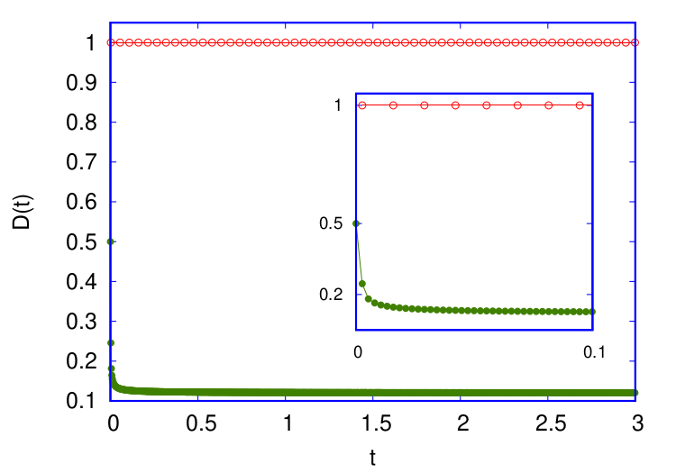
Figure 1: Noise intensity as a function of time for the $2+1$ SS model. The upper curve corresponds to the applied noise while the lower curve to the effective noise, i.e. the noise that actually propagates through the lattice after being filtered by the rules of the SS model. The inset shows the short time behavior.

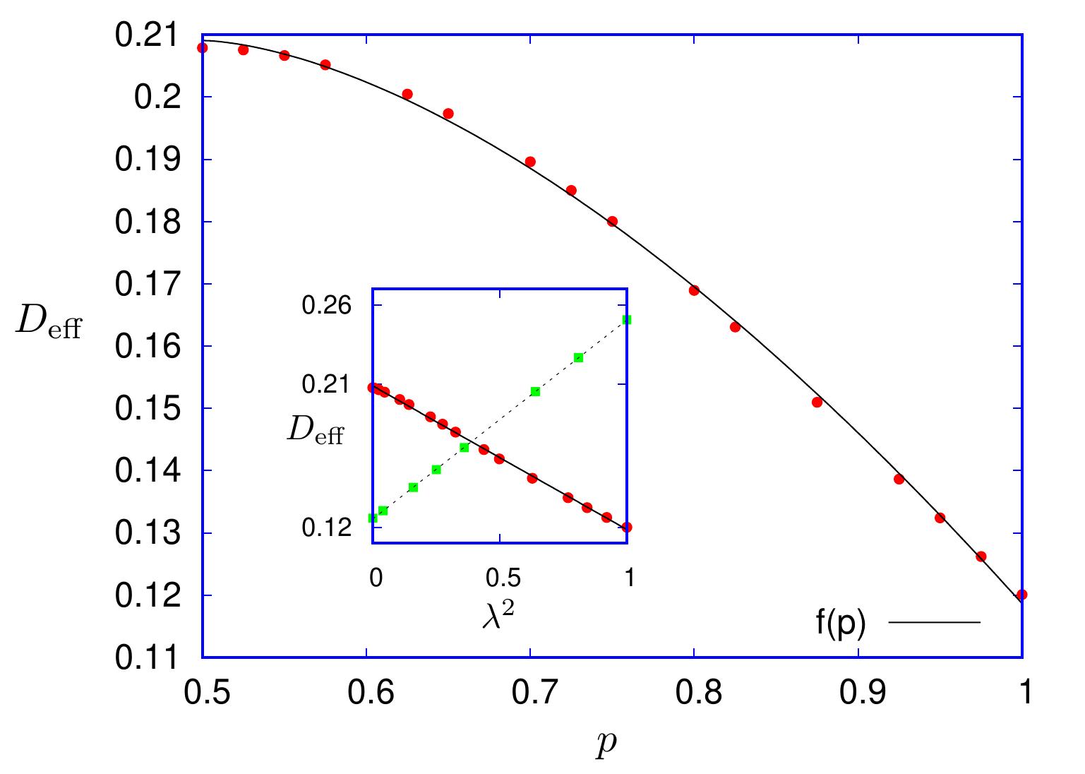
Figure 2: Intensity of the effective noise $D_{eff}$ as a function of $p$ for the SS model in $2+1$ dimensions. The continuous curve is the function $f(p)=c_{1}-c_{2}(p-q)^{\varphi}$. Here $\varphi$ is the golden ratio, $c_{1}$ and $c_{2}$ are adjustable constants. In the inset we have $D_{eff}$ as function of $\lambda^{2}$. The dashed line with positive slope is for $1+1$ dimensions with $\lambda=p-q$ while the other one with negative slope is for $2+1$ dimensions.

Finally, we can generalize the Eq. (13) to obtain a most general form of $w_{s}$ as Gomes-Filho et al. (2021):

$$w_{s}=\left(\frac{D}{b\nu\Phi}L\right)^{\alpha},$$ (15)

and then, we rewrite the FDT as

$$\left\langle\xi(\vec{x},t)\xi(\vec{x^{\prime}},t^{\prime})\right\rangle=2c\nu w_{s}^{1/\alpha}\delta^{(d_{f})}(\vec{x}-\vec{x^{\prime}})\delta(t-t^{\prime}).$$ (16)

Definitions of fractional delta functions can be found in Jumarie (2009); Muslih (2010). For $1+1$ dimensions $\alpha=1/2$ and Eq. (16) reduces to Eq. (14). For $d+1$ dimensions with $d\geqslant 2$, $\alpha$ and $d_{f}$ is given by Eq. (10). Here $c$ is given by $c=\frac{24\Phi}{L}$, where the parameter $\Phi$ is a dimensionless number given by

$$\Phi=\left(\frac{D}{\nu}\right)^{\theta/d_{f}}\left(\frac{\lambda}{\nu}\right)^{\theta},$$ (17)

with $\theta=0$ for $d=1$, thus $\Phi=1$, and a number close to zero for higher dimensions. For $2+1$ dimensions the etching model yields Gomes-Filho et al. (2021) $\Phi=1.00(2)$, for other models $\Phi$ is of the order of unity. It is not necessary that $\Phi$ is of the order of unit, however it sounds strange when a dimensional analysis has hidden numbers that are too big or too small. The Eq. (16) generalizes the result for $1+1$ dimensions Gomes-Filho and Oliveira (2021). This is a step forward, however it should be noted not only that here we have a FDT for each growth equation, but also that the exponent $\alpha$ changes with dimension while the FDT for the Langevin’s equation (12) is very general and independent of the dimension.

Note that Eq. (14) reflects a general characteristic of the FDT of being a linear response to small deviation from equilibrium. This fact is very clear at saturation, thus the nonlinear term is not so important. Note again that going from Eq. (3) to (14) does not alter the KPZ equation. Equation (3) is what is applied while Eq. (14) is what propagates.

IV The hidden symmetry

The breaking of the crystalline structure such as discussed above bring us in a first step to a no man’s land. Next we realize that we have universal values, for example in $2+1$ dimensions $z=d_{f}=\varphi=1.61803...$, we compare this value with experiments in electro-chemically induced co-deposition of nanostructured NiW alloy films, $z=1.6(2)$ Orrillo et al. (2017), dynamics in chemical vapor deposition in silica films, $z=1.6(1)$ Ojeda et al. (2000), on semiconductor polymer deposition $z=1.61(5)$ Almeida et al. (2014) and in excess of mutational jackpot events in expanding populations revealed by spatial Luria–Delbrück experiments, $z=1.61$ Fusco et al. (2016). Thus we have agreement with different kinds of recent experiments, and very precise simulations Gomes-Filho and Oliveira (2021), it is unlikely to be just a numerical coincidence. Consequently, there is a well defined fractal geometry for KPZ and the cellular automata associated with it, whose symmetries are unknown.

The golden ratio $\varphi$ is associated with the limit of the Fibonacci sequence $0,1,1,2,3,5...$ i.e. a sequence where the element of order n is given by $F_{n}=F_{n-1}+F_{n-2}$, thus in the limit $n\rightarrow\infty$ we have the golden ratio $\varphi=\lim_{n\rightarrow\infty}=F_{n+1}/F_{n}$. This sequence is very common in growth forms Dunlap (1997).

Platonic solids and symmetries.— The first place to look for symmetry in $3$ dimensions are the platonic solids. For example, one can consider the icosahedron or its dual, the dodecahedron, both of these solids have a well-known relationship with the golden ratio. The icosahedron consists of $20$ identical equilateral triangular faces, $30$ edges and $12$ vertices. It has a large group of symmetry and it is isomorphic to the non-abelian group $A_{5}$ of all icosahedron rotations Szajewska (2014); Hamermesh (2012). The $A_{5}$ group has one trivial singlet, two triplets, one quartet, and one quintet. In their matricial representation the generators of the triplets and of the quintet has elements where $\varphi^{k}$, with $k=0,1,2$ appears.

Deterministic fractal cellular automata.— Magnetic systems are probability the best physical system to look for symmetry. Even the most simple Ising hamiltonian system exhibit the symmetric paramagnetic phase, and the symmetric breaking phases (ferro and antiferromagnetic). In addition to the trivial phases, is possible to construct additional fractal symmetry protected topological (FSPT) phases via a decorated defect approach (see Devakul et al. (2019) and references there in).

We can define a fractal cellular automaton using the rules of fractal geometry. For example we can take the set of points $i=(....-2,-1,0,1,2,...)$ as an infinite line. The rules

$$a^{t+1}_{i}=a^{t}_{i-1}+a^{t}_{i}+a^{t}_{i+1}\,\,\,{\text{mod}\,2},$$ (18)

with the initial condition $a^{0}_{i}={\delta_{0i}}$, generate a Fibonacci fractal Devakul et al. (2019) in the space-time $(i,t)$. From that we get the (Hausdorff) fractal dimension $d_{f}=1+\log_{2}(\varphi)\approx 1.63$. The golden ratio appears associated with this fractal dimension, however it is not yet the fractal dimension itself.

As a more general example, we can consider the Fibonacci Word Fractal (FWF). This process is more interesting to us because it is a dynamical growth process and consequently more connect with our physical motion, so we shall discuss it briefly. FWF are strings over $\{0,1\}$ defined inductively as follows: $f_{0}=1,f_{1}=0$, $f_{n}=f_{n-1}f_{n-2}$ (i.e. $f_{n}$ is the concatenation of the two previous strings, e.g. $f_{2}=01,f_{3}=010,\cdots$), for $n\geqslant 2$. The FWF can be associated with a curve using the following drawing rule: for each digit at position $k$, draw a segment forward then if the digit is $1$ stay straight, if the digit is $0$, turn $\theta$ radians to the left, when $k$ is even, or turn $\theta$ radians to the right, when $k$ is odd. For an arbitrary $\theta$, Monnerot-Dumaine (2009) shows that

$$d_{f}=\frac{3\ln\varphi}{\ln(1+\cos\theta+\sqrt{(1+\cos\theta)^{2}+1})}.$$

Note that for an adequate choice of the turning angle $\theta$, we can generate a fractal curve with $d_{f}=\varphi$. A simple calculation shows that $\theta\approx 0.9902\frac{\pi}{2}$, i.e almost a right angle.

Figure 3 shows an example of this fractal for a different number of interactions.

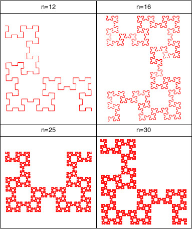
Figure 3: The Fibonacci Word Fractal for a turning angle $\theta\approx 0.9902\frac{\pi}{2}$. This curve has Hausdorff dimension $\varphi$. The result is almost indistinguishable from that of $\theta=\pi/2$. However, if we select $n=30$ and we follow the trajectory around the big white square, we see that the cumulative effects are such that the trajectory does not close.

Stochastic cellular automata.— Now we return to the growth problem described by a stochastic KPZ equation or by a stochastic growth cellular automaton belonging to the KPZ universality class. There are a number of well-known cellular automata and probably much more to be discovered. All of them acts in an integer space of dimensions $D_{i}=d+1$ and generates a fractal space of dimensions $D_{f}=d_{f}+1$, with the same $d_{f}$ given by Eq. (10). The fractal dimension associated with universality via Eq. (8) is itself universal. Therefore, there must be a hidden symmetry and with that new finite non Abelian groups. Is quite natural that we have identified first the groups of perfect crystal, since we have a visual identification of its properties. For fractal which may present only average self-similarity it is more hard to find. However, we expect that soon we would be able to unveiling it. Although we have not yet identified such groups, the discussion above, particularly the concept of self-similarity, is a starting point for such endeavour. Once it is discovered, its importance will be far beyond KPZ.

Conclusion.— In this work, we discuss the fluctuation-dissipation theorem for the Kardar-Parisi-Zhang equation in a space of $d+1$ dimensions. We show how an applied noise is transformed as it goes through the filter imposed by the rules of a cellular automaton. In particular we use the SS model, where controlling the probability $p$ we can change the effective noise intensity. The results support recent work Gomes-Filho et al. (2021), which suggest that the effective noise has fractal dimension $d_{f}$. This fractal dimension is associated with the KPZ exponents from Eq. (10), in such way that we have now not only the triad $(\alpha,\beta,z)$ but the quaternary $(d_{f},\alpha,\beta,z)$. This new universality implies that we have a new hidden symmetry for the KPZ universality class. We found a deterministic cellular automaton from which we can control the Hausdorff dimension $d_{f}$ in such way that, we can obtain $d_{f}=\varphi$. This may be a starting point for new symmetries relations.

Funding

This work was supported by the Conselho Nacional de Desenvolvimento Científico e Tecnológico (CNPq), Grant No. CNPq-312497/2018-0 and the Fundação de Apoio a Pesquisa do Distrito Federal (FAPDF), Grant No. FAPDF- 00193-00000120/2019-79. (F.A.O.).

References

- Edwards and Wilkinson (1982) S. F. Edwards and D. Wilkinson, Proceedings of the Royal Society of London. A. Mathematical and Physical Sciences 381, 17 (1982).
- Kardar et al. (1986) M. Kardar, G. Parisi, and Y.-C. Zhang, Physical Review Letters 56, 889 (1986).
- Barabási and Stanley (1995) A.-L. Barabási and H. E. Stanley, Fractal concepts in surface growth (Cambridge university press, 1995).
- Mello et al. (2001) B. A. Mello, A. S. Chaves, and F. A. Oliveira, Physical Review E 63, 041113 (2001).
- Reis (2005) F. A. Reis, Physical Review E 72, 032601 (2005).
- Almeida et al. (2014) R. Almeida, S. Ferreira, T. Oliveira, and F. A. Reis, Physical Review B 89, 045309 (2014).
- Rodrigues et al. (2014) E. A. Rodrigues, B. A. Mello, and F. A. Oliveira, Journal of Physics A: Mathematical and Theoretical 48, 035001 (2014).
- Alves et al. (2016) W. S. Alves, E. A. Rodrigues, H. A. Fernandes, B. A. Mello, F. A. Oliveira, and I. V. Costa, Physical Review E 94, 042119 (2016).
- Carrasco and Oliveira (2018) I. S. Carrasco and T. J. Oliveira, Physical Review E 98, 010102 (2018).
- Krug et al. (1992) J. Krug, P. Meakin, and T. Halpin-Healy, Physical Review A 45, 638 (1992).
- Krug (1997) J. Krug, Advances in Physics 46, 139 (1997).
- Derrida and Lebowitz (1998) B. Derrida and J. L. Lebowitz, Physical review letters 80, 209 (1998).
- Meakin et al. (1986) P. Meakin, P. Ramanlal, L. M. Sander, and R. Ball, Physical Review A 34, 5091 (1986).
- Daryaei (2020) E. Daryaei, Physical Review E 101, 062108 (2020).
- Hansen et al. (2000) A. Hansen, J. Schmittbuhl, G. G. Batrouni, and F. A. de Oliveira, Geophysical research letters 27, 3639 (2000).
- Merikoski et al. (2003) J. Merikoski, J. Maunuksela, M. Myllys, J. Timonen, and M. J. Alava, Physical review letters 90, 024501 (2003).
- Ódor et al. (2010) G. Ódor, B. Liedke, and K.-H. Heinig, Physical Review E 81, 031112 (2010).
- Takeuchi (2013) K. A. Takeuchi, Physical review letters 110, 210604 (2013).
- Almeida et al. (2017) R. A. Almeida, S. O. Ferreira, I. Ferraz, and T. J. Oliveira, Scientific reports 7, 1 (2017).
- Gwa and Spohn (1992) L.-H. Gwa and H. Spohn, Physical review letters 68, 725 (1992).
- De Vega and Woynarovich (1985) H. De Vega and F. Woynarovich, Nuclear Physics B 251, 439 (1985).
- Plischke et al. (1987) M. Plischke, Z. Rácz, and D. Liu, Physical Review B 35, 3485 (1987).
- Corwin et al. (2018) I. Corwin, P. Ghosal, A. Krajenbrink, P. Le Doussal, and L.-C. Tsai, Physical review letters 121, 060201 (2018).
- Nahum et al. (2017) A. Nahum, J. Ruhman, S. Vijay, and J. Haah, Physical Review X 7, 031016 (2017).
- Ljubotina et al. (2019) M. Ljubotina, M. Žnidarič, and T. Prosen, Physical review letters 122, 210602 (2019).
- De Nardis et al. (2019) J. De Nardis, M. Medenjak, C. Karrasch, and E. Ilievski, Physical review letters 123, 186601 (2019).
- Dasgupta et al. (1996) C. Dasgupta, S. D. Sarma, and J. Kim, Physical Review E 54, R4552 (1996).
- Dasgupta et al. (1997) C. Dasgupta, J. Kim, M. Dutta, and S. D. Sarma, Physical Review E 55, 2235 (1997).
- Torres and Buceta (2018) M. Torres and R. Buceta, Journal of Statistical Mechanics: Theory and Experiment 2018, 033208 (2018).
- Wio et al. (2010) H. S. Wio, J. A. Revelli, R. Deza, C. Escudero, and M. de La Lama, EPL (Europhysics Letters) 89, 40008 (2010).
- Wio et al. (2017) H. S. Wio, Rodríguez, M. A, Gallego, Rafael, J. A. Revelli, A. Alés, and R. R. Deza, Frontiers in Physics 4, 52 (2017).
- Rodríguez and Wio (2019) M. A. Rodríguez and H. S. Wio, Physical Review E 100, 032111 (2019).
- Bertini and Giacomin (1997) L. Bertini and G. Giacomin, Communications in mathematical physics 183, 571 (1997).
- Baik et al. (1999) J. Baik, P. Deift, and K. Johansson, Journal of the American Mathematical Society 12, 1119 (1999).
- Prähofer and Spohn (2000) M. Prähofer and H. Spohn, Physical review letters 84, 4882 (2000).
- Dotsenko (2010) V. Dotsenko, Journal of Statistical Mechanics: Theory and Experiment 2010, P07010 (2010).
- Calabrese et al. (2010) P. Calabrese, P. Le Doussal, and A. Rosso, EPL (Europhysics Letters) 90, 20002 (2010).
- Amir et al. (2011) G. Amir, I. Corwin, and J. Quastel, Communications on pure and applied mathematics 64, 466 (2011).
- Sasamoto and Spohn (2010) T. Sasamoto and H. Spohn, Physical review letters 104, 230602 (2010).
- Le Doussal et al. (2016) P. Le Doussal, Majumdar, N. Satya, A. Rosso, and G. Schehr, Physical review letters 117, 070403 (2016).
- Hairer (2013) M. Hairer, Annals of mathematics , 559 (2013).
- Johansson (2000) K. Johansson, Communications in mathematical physics 209, 437 (2000).
- Gomes-Filho et al. (2021) M. S. Gomes-Filho, A. L. Penna, and F. A. Oliveira, Results in Physics 26, 104435 (2021).
- Brown (1828a) R. Brown, The philosophical magazine 4, 161 (1828a).
- Brown (1828b) R. Brown, Annalen der Physik 90, 294 (1828b).
- Einstein (1905) A. Einstein, Annalen der physik 17, 208 (1905).
- Einstein (1956) A. Einstein, Investigations on the Theory of the Brownian Movement (Courier Corporation, 1956).
- Langevin (1908) P. Langevin, Compt. Rendus 146, 530 (1908).
- Vainstein et al. (2006) M. H. Vainstein, I. V. L. Costa, and F. A. Oliveira, in Jamming, Yielding, and Irreversible Deformation in Condensed Matter (Springer, 2006) pp. 159–188.
- Gudowska-Nowak et al. (2017) E. Gudowska-Nowak, K. Lindenberg, and R. Metzler, Journal of Physics A: Mathematical and Theoretical 50, 380301 (2017).
- Oliveira et al. (2019) F. A. Oliveira, R. M. S. Ferreira, L. C. Lapas, and M. H. Vainstein, Frontiers in Physics 7, 18 (2019).
- Onsager (1931) L. Onsager, Physical review 37, 405 (1931).
- Gomes-Filho and Oliveira (2021) M. S. Gomes-Filho and F. A. Oliveira, EPL (Europhysics Letters) 133, 10001 (2021).
- Grigera and Israeloff (1999) T. S. Grigera and N. Israeloff, Physical Review Letters 83, 5038 (1999).
- Ricci-Tersenghi et al. (2000) F. Ricci-Tersenghi, D. A. Stariolo, and J. J. Arenzon, Physical review letters 84, 4473 (2000).
- Crisanti and Ritort (2003) A. Crisanti and F. Ritort, Journal of Physics A: Mathematical and General 36, R181 (2003).
- Barrat (1998) A. Barrat, Physical Review E 57, 3629 (1998).
- Bellon and Ciliberto (2002) L. Bellon and S. Ciliberto, Physica D: Nonlinear Phenomena 168, 325 (2002).
- Bellon et al. (2006) L. Bellon, L. Buisson, M. Ciccotti, S. Ciliberto, and F. Douarche, in Jamming, Yielding, and Irreversible Deformation in Condensed Matter (Springer, 2006) pp. 23–52.
- Hayashi and Takano (2007) K. Hayashi and M. Takano, Biophysical journal 93, 895 (2007).
- Pérez-Madrid et al. (2009) A. Pérez-Madrid, L. C. Lapas, and J. M. Rubí, Physical review letters 103, 048301 (2009).
- Averin and Pekola (2010) D. V. Averin and J. P. Pekola, Physical review letters 104, 220601 (2010).
- Costa et al. (2003) I. V. Costa, R. Morgado, M. V. Lima, and F. A. Oliveira, EPL (Europhysics Letters) 63, 173 (2003).
- Costa et al. (2006) I. V. Costa, M. H. Vainstein, L. C. Lapas, A. A. Batista, and F. A. Oliveira, Physica A: Statistical Mechanics and its Applications 371, 130 (2006).
- Lapas et al. (2007) L. Lapas, I. Costa, M. Vainstein, and F. Oliveira, EPL (Europhysics Letters) 77, 37004 (2007).
- Lapas et al. (2008) L. C. Lapas, R. Morgado, M. H. Vainstein, J. M. Rubí, and F. A. Oliveira, Physical review letters 101, 230602 (2008).
- Gomes et al. (2019) W. P. Gomes, A. L. Penna, and F. A. Oliveira, Physical Review E 100, 020101 (2019).
- Jumarie (2009) G. Jumarie, Applied Mathematics Letters 22, 1659 (2009).
- Muslih (2010) S. I. Muslih, International Journal of Theoretical Physics 49, 2095 (2010).
- Orrillo et al. (2017) P. A. Orrillo, S. N. Santalla, R. Cuerno, L. Vázquez, S. B. Ribotta, L. M. Gassa, F. Mompean, R. C. Salvarezza, and M. E. Vela, Scientific reports 7, 1 (2017).
- Ojeda et al. (2000) F. Ojeda, R. Cuerno, R. Salvarezza, and L. Vázquez, Physical review letters 84, 3125 (2000).
- Fusco et al. (2016) D. Fusco, M. Gralka, J. Kayser, A. Anderson, and O. Hallatschek, Nature communications 7, 1 (2016).
- Dunlap (1997) R. A. Dunlap, The golden ratio and Fibonacci numbers (World Scientific, 1997).
- Szajewska (2014) M. Szajewska, Acta Crystallographica Section A: Foundations and Advances 70, 358 (2014).
- Hamermesh (2012) M. Hamermesh, Group theory and its application to physical problems (Courier Corporation, 2012).
- Devakul et al. (2019) T. Devakul, Y. You, F. Burnell, and S. Sondhi, SciPost Phys 6 (2019).
- Monnerot-Dumaine (2009) A. Monnerot-Dumaine, “The Fibonacci Word fractal,” (2009), 24 pages, 25 figures.