How to exploit hyperspherical embeddings for out-of-distribution detection?

Abstract

Out-of-distribution (OOD) detection is a critical task for reliable machine learning. Recent advances in representation learning give rise to distance-based OOD detection, where testing samples are detected as OOD if they are relatively far away from the centroids or prototypes of in-distribution (ID) classes. However, prior methods directly take off-the-shelf contrastive losses that suffice for classifying ID samples, but are not optimally designed when test inputs contain OOD samples. In this work, we propose CIDER, a novel representation learning framework that exploits hyperspherical embeddings for OOD detection. CIDER jointly optimizes two losses to promote strong ID-OOD separability: a dispersion loss that promotes large angular distances among different class prototypes, and a compactness loss that encourages samples to be close to their class prototypes. We analyze and establish the unexplored relationship between OOD detection performance and the embedding properties in the hyperspherical space, and demonstrate the importance of dispersion and compactness. CIDER establishes superior performance, outperforming the latest rival by 13.33% in FPR95. Code is available at https://github.com/deeplearning-wisc/cider.

1 Introduction

When deploying machine learning models in the open world, it is important to ensure the reliability of the model in the presence of out-of-distribution (OOD) inputs—samples from an unknown distribution that the network has not been exposed to during training, and therefore should not be predicted with high confidence at test time. We desire models that are not only accurate when the input is drawn from the known distribution, but are also aware of the unknowns outside the training categories. This gives rise to the task of OOD detection, where the goal is to determine whether an input is in-distribution (ID) or not.

A plethora of OOD detection algorithms have been developed recently, among which distance-based methods demonstrated promise (Lee et al., 2018; Xing et al., 2020). These approaches circumvent the shortcoming of using the model’s confidence score for OOD detection, which can be abnormally high on OOD samples (Nguyen et al., 2015) and hence not distinguishable from ID data. Distance-based methods leverage feature embeddings extracted from a model, and operate under the assumption that the test OOD samples are relatively far away from the clusters of ID data.

Arguably, the efficacy of distance-based approaches can depend largely on the quality of feature embeddings. Recent works including SSD+ (Sehwag et al., 2021) and KNN+ (Sun et al., 2022) directly employ off-the-shelf contrastive losses for OOD detection. In particular, these works use the supervised contrastive loss (SupCon) (Khosla et al., 2020) for learning the embeddings, which are then used for OOD detection with either parametric Mahalanobis distance (Lee et al., 2018; Sehwag et al., 2021) or non-parametric KNN distance (Sun et al., 2022). However, existing training objectives produce embeddings that suffice for classifying ID samples, but remain sub-optimal for OOD detection. For example, when trained on CIFAR-10 using SupCon loss, the average angular distance between ID and OOD data is only 29.86 degrees in the embedding space, which is too small for effective ID-OOD separation. This raises the important question:

How to exploit representation learning methods that maximally benefit OOD detection?

In this work, we propose CIDER, a Compactness and DispErsion Regularized learning framework designed for OOD detection. Our method is motivated by the desirable properties of hyperspherical embeddings, which can be naturally modeled by the von Mises-Fisher (vMF) distribution. vMF is a classical and important distribution in directional statistics (Mardia et al., 2000), is analogous to spherical Gaussian distributions for features with unit norms. Our key idea is to design an end-to-end trainable loss function that enables optimizing hyperspherical embeddings into a mixture of vMF distributions, which satisfy two properties simultaneously: (1) each sample has a higher probability assigned to the correct class in comparison to incorrect classes, and (2) different classes are far apart from each other. To formalize our idea, CIDER introduces two losses: a dispersion loss that promotes large angular distances among different class prototypes, along with a compactness loss that encourages samples to be close to their class prototypes. These two terms are complementary to shape hyperspherical embeddings for both OOD detection and ID classification purposes. Unlike previous contrastive loss, CIDER explicitly formalizes the latent representations as vMF distributions, thereby providing a direct theoretical interpretation of hyperspherical embeddings.

In particular, we show that promoting large inter-class dispersion is key to strong OOD detection performance, which has not been explored in previous literature. Previous methods including SSD+ directly use off-the-shelf SupCon loss, which produces embeddings that lack sufficient inter-class dispersion needed for OOD detection. CIDER mitigates the issue by explicitly optimizing for large inter-class margins and leads to more desirable hyperspherical embeddings. Noticeably, when trained on CIFAR-10, CIDER displays a relative 42.36% improvement of ID-OOD separability compared to SupCon. We further show that CIDER’s strong representation can benefit different distance-based OOD scores, outperforming recent competitive methods SSD+ (Sehwag et al., 2021) and KNN+ (Sun et al., 2022) by a significant margin. Our key results and contributions are:

1. We propose CIDER, a novel representation learning framework designed for OOD detection. Compared to the latest rival (Sun et al., 2022), CIDER produces superior embeddings that lead to 13.33% error reduction (in FPR95) on the challenging CIFAR-100 benchmark.

2. We are the first to establish the unexplored relationship between OOD detection performance and the embedding quality in the hyperspherical space, and provide measurements based on the notion of compactness and dispersion. This allows future research to quantify the embedding in the hyperspherical space for effective OOD detection.

3. We offer new insights on the design of representation learning for OOD detection. We also conduct extensive ablations to understand the efficacy and behavior of CIDER, which remains effective and competitive under various settings, including the ImageNet dataset.

2 Preliminaries

We consider multi-class classification, where $\mathcal{X}$ denotes the input space and $\mathcal{Y}^{\text{in}}=\{1,2,...,C\}$ denotes the ID labels. The training set $\mathcal{D}_{\text{tr}}^{\text{in}}=\{(\mathbf{x}_{i},y_{i})\}_{i=1}^{N}$ is drawn i.i.d. from $P_{\mathcal{X}\mathcal{Y}^{\text{in}}}$. Let $P_{\mathcal{X}}$ denote the marginal distribution over $\mathcal{X}$, which is called the in-distribution (ID).

Out-of-distribution detection. OOD detection can be viewed as a binary classification problem. At test time, the goal of OOD detection is to decide whether a sample $\mathbf{x}\in\mathcal{X}$ is from $P_{\mathcal{X}}$ (ID) or not (OOD). In practice, OOD is often defined by a distribution that simulates unknowns encountered during deployment, such as samples from an irrelevant distribution whose label set has no intersection with $\mathcal{Y}^{\text{in}}$ and therefore should not be predicted by the model. Mathematically, let $\mathcal{D}^{\text{ood}}_{\text{test}}$ denote an OOD test set where the label space $\mathcal{Y}^{\text{ood}}\cap\mathcal{Y}^{\text{in}}=\emptyset$. The decision can be made via a level set estimation: $G_{\lambda}(\mathbf{x})=\mathbbm{1}\{S(\mathbf{x})\geq\lambda\}$, where samples with higher scores $S(\mathbf{x})$ are classified as ID and vice versa. The threshold $\lambda$ is typically chosen so that a high fraction of ID data (e.g. 95%) is correctly classified.

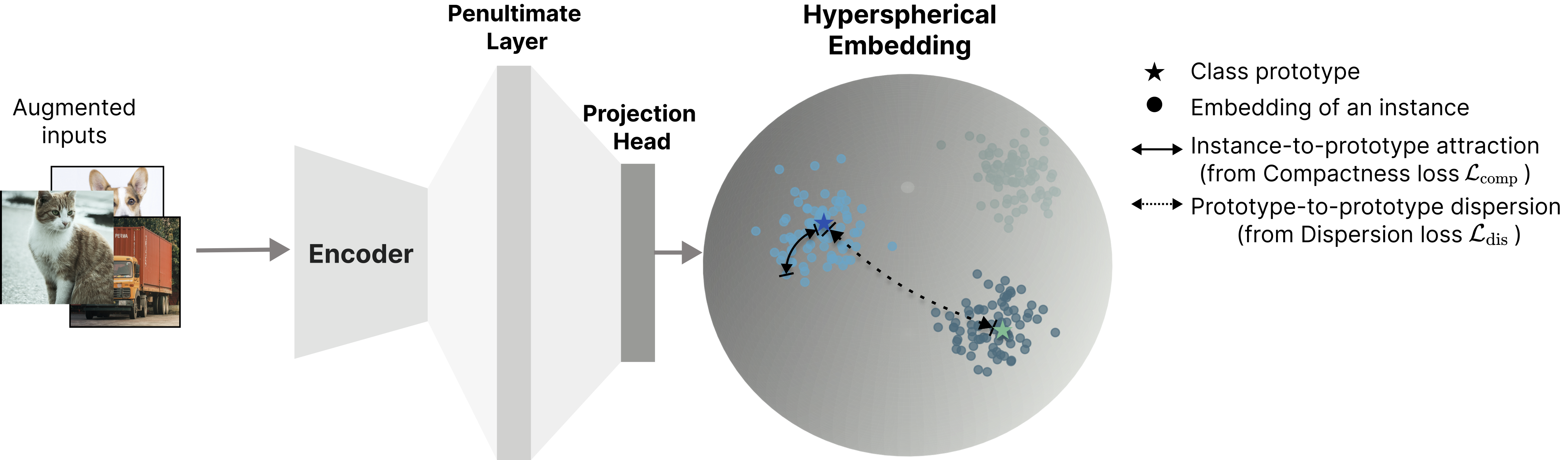
Figure 1: Overview of our compactness and dispersion regularized (CIDER) learning framework for OOD detection. We jointly optimize two complementary terms to encourage desirable properties of the embedding space: (1) a dispersion loss to encourage larger angular distances among different class prototypes, and (2) a compactness loss to encourage samples to be close to their class prototypes.

Hyperspherical embeddings.

A hypersphere is a topological space that is homeomorphic to a standard $n$-sphere, which is the set of points in $(n+1)$-dimensional Euclidean space that are located at a constant distance from the center. When the sphere has a unit radius, it is called the unit hypersphere. Formally, an $n$-dimensional unit-hypersphere $S^{n}:=\{\mathbf{z}\in\mathbb{R}^{n+1}|\lVert\mathbf{z}\rVert_{2}=1\}$. Geometrically, hyperspherical embeddings lie on the surface of a hypersphere.

3 Method

Overview. Our framework CIDER is illustrated in Figure 1. The general architecture consists of two components: (1) a deep neural network encoder $f:\mathcal{X}\mapsto\mathbb{R}^{e}$ that maps the augmented input $\tilde{\mathbf{x}}$ to a high dimensional feature embedding $f(\tilde{\mathbf{x}})$ (often referred to as the penultimate layer features); (2) a projection head $h:\mathbb{R}^{e}\mapsto\mathbb{R}^{d}$ that maps the high dimensional embedding $f(\tilde{\mathbf{x}})$ to a lower dimensional feature representation $\tilde{\mathbf{z}}:=h(f(\tilde{\mathbf{x}}))$. The loss is applied to the normalized feature embedding $\mathbf{z}:=\tilde{\mathbf{z}}/\lVert\tilde{\mathbf{z}}\rVert_{2}$. The normalized embeddings are also referred to as hyperspherical embeddings, since they are on a unit hypersphere. Our goal is to shape the hyperspherical embedding space so that the learned embeddings can be mostly effective for distinguishing ID vs. OOD data.

3.1 model hyperspherical embeddings

The hyperspherical embeddings can be naturally modeled by the von Mises-Fisher (vMF) distribution, a classical and important distribution in directional statistics (Mardia et al., 2000). In particular, vMF is analogous to spherical Gaussian distributions for features $\mathbf{z}$ with unit norms ($\|\mathbf{z}\|^{2}=1$). The probability density function for a unit vector $\mathbf{z}\in\mathbb{R}^{d}$ in class $c$ is defined as:

$$p_{d}(\mathbf{z};\bm{\mu}_{c},\kappa)=Z_{d}(\kappa)\exp\left(\kappa\bm{\mu}_{c}^{\top}\mathbf{z}\right),$$ (1)

where $\bm{\mu}_{c}$ is the class prototype with unit norm, $\kappa\geq 0$ indicates the tightness of the distribution around the mean direction $\bm{\mu}_{c}$, and $Z_{d}(\kappa)$ is the normalization factor. The larger value of $\kappa$, the stronger the distribution is concentrated in the mean direction. In the extreme case of $\kappa=0$, the sample points are distributed uniformly on the hypersphere.

Under this probability model, an embedding vector $\mathbf{z}$ is assigned to class $c$ with the following normalized probability:

$$\mathbb{P}(y=c|\mathbf{z};\{\kappa,\bm{\mu}_{j}\}_{j=1}^{C}) =\frac{Z_{d}\left(\kappa\right)\exp\left(\kappa\bm{\mu}_{c}^{\top}\mathbf{z}\right)}{\sum_{j=1}^{C}Z_{d}\left(\kappa\right)\exp\left(\kappa\bm{\mu}_{j}^{\top}\mathbf{z}\right)}$$ (2)

$$=\frac{\exp\left(\bm{\mu}_{c}^{\top}\mathbf{z}/\tau\right)}{\sum_{j=1}^{C}\exp\left(\bm{\mu}_{j}^{\top}\mathbf{z}/\tau\right)},$$ (3)

where $\kappa={1\over\tau}$. Next, we outline our proposed training method that promotes class-conditional vMF distributions for OOD detection.

3.2 How to optimize Hyperspherical Embeddings?

Training objective. Our key idea is to design a trainable loss function that enables optimizing hyperspherical embeddings into a mixture of vMF distributions, which satisfy two properties simultaneously: (1) each sample has a higher probability assigned to the correct class in comparison to incorrect classes, and (2) different classes are far apart from each other.

To achieve , we can perform maximum likelihood estimation (MLE) on the training data:

$$\text{argmax}_{\theta} \prod_{i=1}^{N}p(y_{i}|\mathbf{z}_{i};\{\kappa_{j},\bm{\mu}_{j}\}_{j=1}^{C}),$$ (4)

where $i$ is the index of the embedding and $N$ is the size of the training set. By taking the negative log-likelihood, the objective function is equivalent to minimizing the following loss:

$$\mathcal{L}_{\mathrm{comp}}=-\frac{1}{N}\sum_{i=1}^{N}\log\frac{\exp\left(\mathbf{z}_{i}^{\top}{\bm{\mu}}_{c(i)}/\tau\right)}{\sum_{j=1}^{C}\exp\left(\mathbf{z}_{i}^{\top}{\bm{\mu}}_{j}/\tau\right)},$$ (5)

where $c(i)$ denotes the class index of a sample $\mathbf{x}_{i}$, and $\tau$ is the temperature parameter. We term this compactness loss, since it encourages samples to be closely aligned with its class prototype.

To promote property , we propose the dispersion loss, optimizing large angular distances among different class prototypes:

$$\mathcal{L}_{\mathrm{dis}}={1\over C}\sum_{i=1}^{C}\log{1\over C-1}\sum_{j=1}^{C}\mathbbm{1}\{j\neq i\}e^{{\bm{\mu}}_{i}^{\top}{\bm{\mu}}_{j}/\tau}.$$ (6)

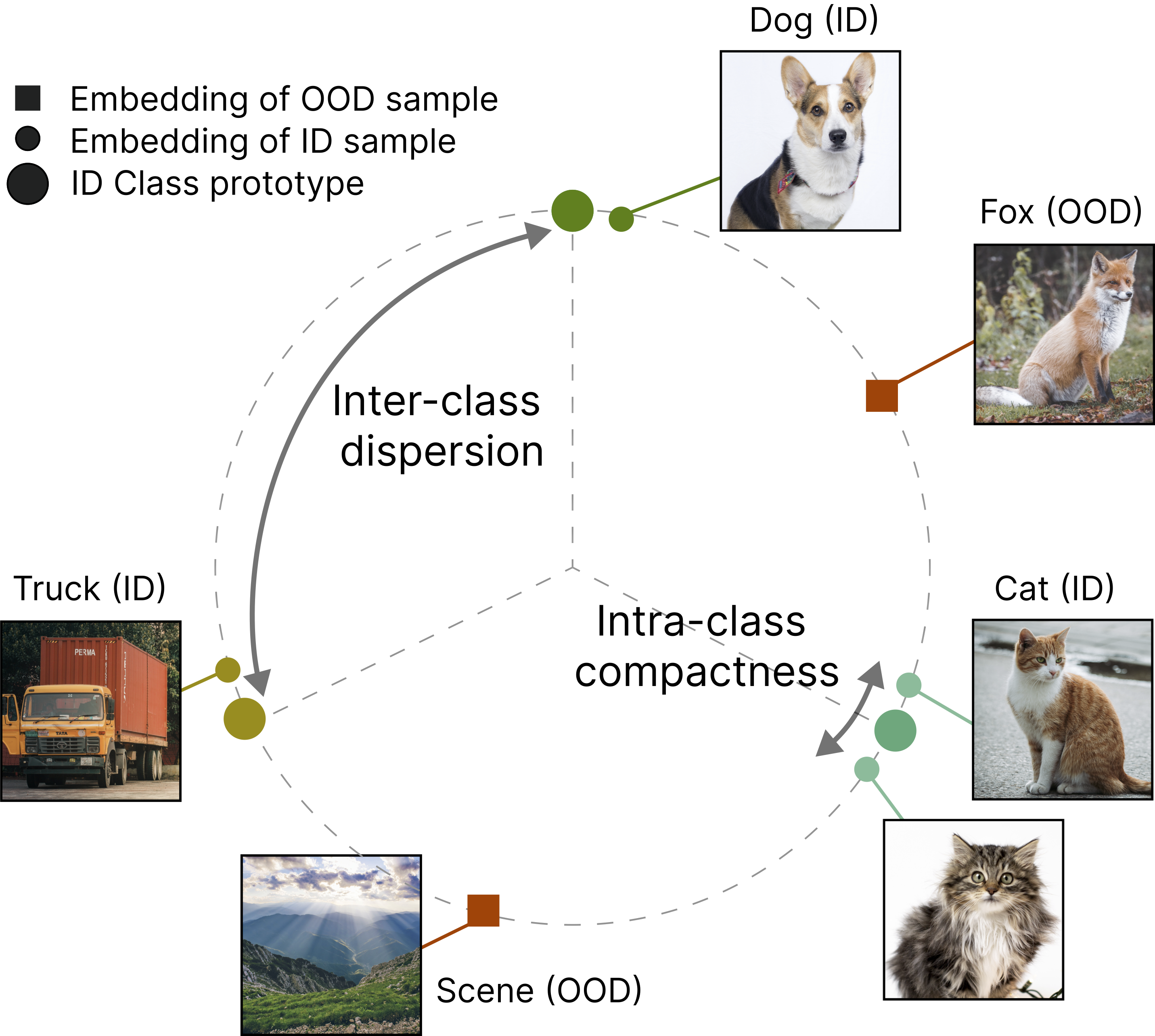
Figure 2: Illustration of desirable hyperspherical embeddings for OOD detection. As OOD samples lie between ID clusters, optimizing a large angular distance among ID clusters benefits OOD detection.

While prototypes with larger pairwise angular distances may not impact ID classification accuracy, they are crucial for OOD detection, as we will show later in Section 4.2. Since the embeddings of OOD samples lie in-between ID clusters, optimizing large inter-class margin benefits OOD detection. The importance of inter-class dispersion can also be explained in Figure 2, where samples in the fox class (OOD) are semantically close to cat (ID) and dog (ID). A larger angular distance (i.e. smaller cosine similarity) between ID classes cat and dog in the hyperspherical space improves the separability from fox, and allows for more effective detection. We investigate this phenomenon quantitatively in Section 4.

Formally, our training objective CIDER (compactness and dispersion regularized learning) is:

$$\mathcal{L}_{\text{CIDER}}=\mathcal{L}_{\mathrm{dis}}+\lambda_{c}\mathcal{L}_{\mathrm{comp}},$$ (7)

where $\lambda_{c}$ is the co-efficient modulating the relative importance of two losses. These two terms are complementary to shape hyperspherical embeddings for both ID classification and OOD detection.

Prototype estimation and update.

During training, an important step is to estimate the class prototype $\bm{\mu}_{c}$ for each class $c\in\{1,2,...,C\}$. One canonical way to estimate the prototypes is to use the mean vector of all training samples for each class and update it frequently during training. Despite its simplicity, this method incurs a heavy computational toll and causes undesirable training latency. Instead, the class-conditional prototypes can be effectively updated in an exponential-moving-average manner (EMA) (Li et al., 2020):

$${\bm{\mu}}_{c}:=\text{Normalize}(\alpha{\bm{\mu}}_{c}+(1-\alpha)\mathbf{z}),\;\forall c\in\{1,2,\ldots,C\}$$ (8)

where the prototype $\bm{\mu}_{c}$ for class $c$ is updated during training as the moving average of all embeddings with label $c$, and $\mathbf{z}$ denotes the normalized embedding of samples of class $c$. We ablate the effect of prototype update factor $\alpha$ in Section C. The pseudo-code for our method is in Appendix A.

Remark 1: Differences w.r.t. SSD+. We highlight three fundamental differences w.r.t. SSD+, in terms of training objective, test-time OOD detection, and theoretical interpretation. (1) At training time, SSD+ directly uses off-the-shelf SupCon loss (Khosla et al., 2020), which produces embeddings that lack sufficient inter-class dispersion needed for OOD detection. For example, when trained on CIFAR-10 using SupCon loss, the average angular distance between ID and OOD data is only 29.86 degrees in the embedding space. In contrast, CIDER enforces the inter-class dispersion by explicitly maximizing the angular distances among different ID class prototypes. As we will show in Section 4.2, CIDER displays a relative 42.36% improvement of ID-OOD separability compared to SSD+, due to the explicit inter-class dispersion. (2) At test time, SSD+ uses the Mahalanobis distance (Lee et al., 2018), which imposes a strong Gaussian distribution assumption on hyperspherical embeddings. In contrast, CIDER alleviates this assumption with a non-parametric distance score. (3) Lastly, CIDER explicitly models the latent representations as vMF distributions, providing a direct and clear geometrical interpretation of hyperspherical embeddings.

Remark 2: Differences w.r.t. Proxy-based methods. Our work also bears significant differences w.r.t. proxy-based metric learning methods. (1) Our primary task is OOD detection, whereas deep metric learning is commonly used for face verification and image retrieval tasks; (2) Prior methods such as ProxyAnchor (Kim et al., 2020) lack explicit prototype-to-prototype dispersion, which we show is crucial for OOD detection. Moreover, ProxyAnchor initializes the proxies randomly and updates through gradients, while we estimate prototypes directly from sample embeddings using EMA. We provide experimental comparisons next.

4 Experiments

4.1 Common Setup

Datasets and training details. Following the common benchmarks in the literature, we consider CIFAR-10 and CIFAR-100 (Krizhevsky et al., 2009) as in-distribution datasets. For OOD test datasets, we use a suite of natural image datasets including SVHN (Netzer et al., 2011), Places365 (Zhou et al., 2017), Textures (Cimpoi et al., 2014b), LSUN  (Yu et al., 2015), and iSUN (Xu et al., 2015). In our main experiments, we use ResNet-18 as the backbone for CIFAR-10 and ResNet-34 for CIFAR-100. We train the model using stochastic gradient descent with momentum 0.9, and weight decay $10^{-4}$. To demonstrate the simplicity and effectiveness of CIDER, we adopt the same hyperparameters as in SSD+ (Sehwag et al., 2021) with the SupCon loss: the initial learning rate is $0.5$ with cosine scheduling, the batch size is $512$, and the training time is $500$ epochs. We choose the default weight $\lambda_{c}=2$, so that the value of different loss terms are similar upon model initialization. Following the literature (Khosla et al., 2020), we use the embedding dimension of 128 for the projection head. The temperature $\tau$ is $0.1$. We adjust the prototype update factor $\alpha$, batch size, temperature, loss weight, prototype update factor, and model architecture in our ablation study (Appendix C). We report the ID classification results for SSD+ and CIDER following the common linear evaluation protocol (Khosla et al., 2020), where a linear classifier is trained on top of the normalized penultimate layer features. More experimental details are provided in Appendix B. Code and data is released publicly for reproducible research.

OOD detection scores. During test time, we employ a distance-based method for OOD detection. An input $\mathbf{x}$ is considered OOD if it is relatively far from the ID data in the embedding space. By default, we adopt a simple non-parametric KNN distance (Sun et al., 2022), which does not impose any distributional assumption on the feature space. Here the distance is the cosine similarity with respect to the $k$-th nearest neighbor, which is equivalent to the (negated) Euclidean distance as all features have unit norms. In the ablation study, we also consider the commonly used Mahalanobis score (Lee et al., 2018) for a fair comparison with SSD+ (Sehwag et al., 2021).

Evaluation metrics. We report the following metrics: (1) the false positive rate (FPR95) of OOD samples when the true positive rate of ID samples is at 95%, (2) the area under the receiver operating characteristic curve (AUROC), and (3) ID classification accuracy (ID ACC).

4.2 Main Results and Analysis

Table 1: OOD detection performance for CIFAR-100 (ID) with ResNet-34. Training with CIDER significantly improves OOD detection performance.

Method	OOD Dataset										Average
	SVHN		Places365		LSUN		iSUN		Texture
	FPR$\downarrow$	AUROC$\uparrow$	FPR$\downarrow$	AUROC$\uparrow$	FPR$\downarrow$	AUROC$\uparrow$	FPR$\downarrow$	AUROC$\uparrow$	FPR$\downarrow$	AUROC$\uparrow$	FPR$\downarrow$	AUROC$\uparrow$
	Without Contrastive Learning
MSP	78.89	79.80	84.38	74.21	83.47	75.28	84.61	74.51	86.51	72.53	83.12	75.27
ODIN	70.16	84.88	82.16	75.19	76.36	80.10	79.54	79.16	85.28	75.23	78.70	79.11
Mahalanobis	87.09	80.62	84.63	73.89	84.15	79.43	83.18	78.83	61.72	84.87	80.15	79.53
Energy	66.91	85.25	81.41	76.37	59.77	86.69	66.52	84.49	79.01	79.96	70.72	82.55
GODIN	74.64	84.03	89.13	68.96	93.33	67.22	94.25	65.26	86.52	69.39	87.57	70.97
LogitNorm	59.60	90.74	80.25	78.58	81.07	82.99	84.19	80.77	86.64	75.60	78.35	81.74
	With Contrastive Learning
ProxyAnchor	87.21	82.43	70.10	79.84	37.19	91.68	70.01	84.96	65.64	84.99	66.03	84.78
CE + SimCLR	24.82	94.45	86.63	71.48	56.40	89.00	66.52	83.82	63.74	82.01	59.62	84.15
CSI	44.53	92.65	79.08	76.27	75.58	83.78	76.62	84.98	61.61	86.47	67.48	84.83
SSD+	31.19	94.19	77.74	79.90	79.39	85.18	80.85	84.08	66.63	86.18	67.16	85.90
KNN+	39.23	92.78	80.74	77.58	48.99	89.30	74.99	82.69	57.15	88.35	60.22	86.14
CIDER	23.09	95.16	79.63	73.43	16.16	96.33	71.68	82.98	43.87	90.42	46.89	87.67

CIDER outperforms competitive approaches. Table 1 contains a wide range of competitive methods for OOD detection. All methods are trained on ResNet-34 using CIFAR-100, without assuming access to auxiliary outlier datasets. For clarity, we divide the methods into two categories: trained with and without contrastive losses. For pre-trained model-based scores such as MSP (Hendrycks & Gimpel, 2017), ODIN (Liang et al., 2018), Mahalanobis (Lee et al., 2018), and Energy (Liu et al., 2020), the model is trained with the softmax cross-entropy (CE) loss. GODIN (Hsu et al., 2020) is trained using the DeConf-C loss, while LogitNorm (Wei et al., 2022) modifies CE loss via logit normalization. For methods involving contrastive losses, we consider ProxyAnchor (Kim et al., 2020), SimCLR (Winkens et al., 2020), CSI (Tack et al., 2020), SSD+ (Sehwag et al., 2021), and KNN+ (Sun et al., 2022). Both SSD+ and KNN+ use the SupCon loss in training. We use the same network structure and embedding dimension, while varying the training objective.

As shown in Table 1, OOD detection performance is significantly improved with CIDER. Three trends can be observed: (1) Compared to SSD+ and KNN+, CIDER explicitly optimizes for inter-class dispersion and leads more desirable embeddings. Moreover, CIDER alleviates the class-conditional Gaussian assumptions for OOD detection. Instead, a simple non-parametric distance-based score suffices. Specifically, CIDER outperforms the competitive methods SSD+ by 20.3% and KNN+ by 13.3% in FPR95; (2) While CSI (Tack et al., 2020) relies on sophisticated data augmentations and ensembles in testing, CIDER only uses the default data augmentations and thus is simpler in practice. Performance wise, CIDER reduces the average FPR95 by $20.6\%$ compared to CSI; (3) Lastly, as a result of the improved embedding quality, CIDER improves the ID accuracy by $0.76\%$ compared to training with the CE loss (Table 9). We provide results on the less challenging task (CIFAR-10 as ID) in Appendix E, where CIDER’s strong performance remains.

CIDER benefits different distance-based scores. We show that CIDER’s strong representation can benefit different distance-based OOD scores. We consider the Mahalanobis score (denoted as Maha) due to its commonality, and to ensure a fair comparison with SSD+ under the same OOD score. The results are shown in Table 2. Under both KNN (non-parametric) and Maha (parametric) scores, CIDER consistently improves the OOD detection performance compared to training with SupCon. For example, CIDER with KNN significant reduces FPR95 by $\textbf{13.33}\%$ compared to SupCon+KNN. Moreover, compared to SSD+ (SupCon+Maha), CIDER+Maha reduces FPR95 by $\textbf{22.77}\%$. This further highlights the improved representation quality and generality of CIDER.

Table 2: Ablation on OOD detection score. Results are FPR95 on CIFAR-100 (ID) with ResNet-34. We evaluate both Mahalanobis and KNN score ($K=300$).

Method	OOD Dataset					AVG FPR95
	SVHN	Places365	LSUN	iSUN	Texture
SupCon+Maha (SSD+)	31.19	77.74	79.39	80.85	66.63	67.16
CIDER+Maha	16.68	80.34	11.07	73.82	40.06	44.39
SupCon+KNN (KNN+)	39.23	80.74	48.99	74.99	57.15	60.22
CIDER+KNN	23.09	79.63	16.16	71.68	43.87	46.89

Inter-class dispersion is key to strong OOD detection.

Here we examine the effects of loss components on OOD detection. As shown in Table 3, we have the following observations: (1) For ID classification, training with $\mathcal{L}_{\mathrm{comp}}$ alone leads to an accuracy of $75.19\%$, similar to the ID accuracy of SSD+ ($75.11\%$). This suggests that promoting intra-class compactness and a moderate level of inter-class dispersion (as a result of sample-to-prototype negative pairs in $\mathcal{L}_{\mathrm{comp}}$) are sufficient to discriminate different ID classes; (2) For OOD detection, further inter-class dispersion is critical, which is explicitly encouraged through the dispersion loss $\mathcal{L}_{\mathrm{dis}}$. As a result, adding $\mathcal{L}_{\mathrm{dis}}$ improved the average AUROC by $2\%$. However, promoting inter-class dispersion via $\mathcal{L}_{\mathrm{dis}}$ alone without $\mathcal{L}_{\mathrm{comp}}$ is not sufficient for neither ID classification nor OOD detection. Our ablation suggests that $\mathcal{L}_{\mathrm{dis}}$ and $\mathcal{L}_{\mathrm{comp}}$ work synergistically to improve the hyperspherical embeddings that are desirable for both ID classification and OOD detection.

Table 3: Ablation study on loss component. Results (in AUROC) are based on CIFAR-100 trained with ResNet-34. Training with only $\mathcal{L}_{\mathrm{comp}}$ suffices for ID classification. Inter-class dispersion induced by $\mathcal{L}_{\mathrm{dis}}$ is key to OOD detection.

Loss Components		AUROC$\uparrow$						ID ACC$\uparrow$
$\mathcal{L}_{\mathrm{comp}}$	$\mathcal{L}_{\mathrm{dis}}$	Places365	LSUN	iSUN	Texture	SVHN	AVG
$\checkmark$		79.63	85.75	84.45	87.21	91.33	85.67	75.19
	$\checkmark$	54.76	69.81	54.99	44.26	46.48	54.06	2.03
$\checkmark$	$\checkmark$	73.43	96.33	82.98	90.42	95.16	87.67	75.35

4.3 Characterizing and Understanding Embedding Quality

CIDER learns distinguishable representations. We visualize the learned feature embeddings in Figure 3 using UMAP (McInnes et al., 2018), where the colors encode different class labels. A salient observation is that embeddings obtained with CIDER enjoy much better compactness compared to embeddings trained with the CE loss (3(a)). Moreover, the classes are distributed more uniformly in the space, highlighting the efficacy of the dispersion loss.

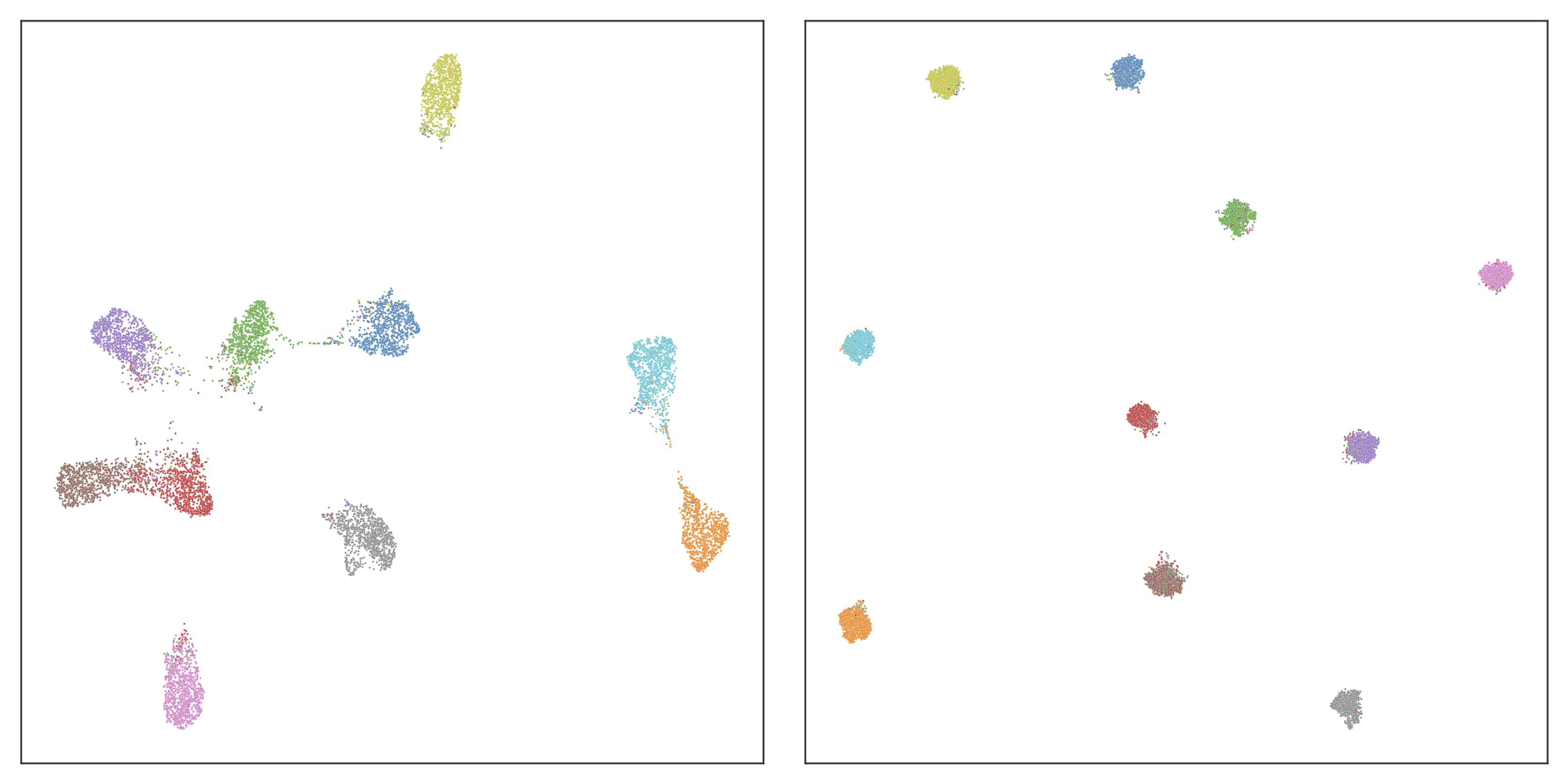
(a) ID embeddings of CE (left) and CIDER (right)

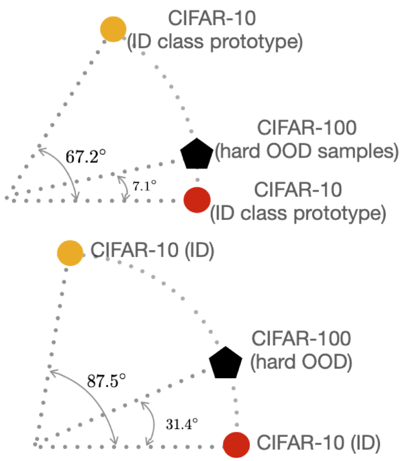
(b) ID & OOD of CE (top) and CIDER (down)

Figure 3: (a): UMAP (McInnes et al., 2018) visualization of the features when the model is trained with CE vs. CIDER for CIFAR-10 (ID). (b): CIDER makes OOD samples more separable from ID compared to CE (c.f. Table 4).

CIDER improves inter-class dispersion and intra-class compactness. Beyond visualization, we also quantitatively measure the embedding quality. We propose two measurements: inter-class dispersion and intra-class compactness:

$$\text{Dispersion}({\bm{\mu}})={1\over C}\sum_{i=1}^{C}{1\over C-1}\sum_{j=1}^{C}{{\bm{\mu}}_{i}^{\top}{\bm{\mu}}_{j}}\mathbbm{1}\{j\neq i\}.$$

$$\text{Compactness}(\mathcal{D}_{\text{tr}}^{\text{in}},{\bm{\mu}})={1\over C}\sum_{j=1}^{C}{1\over n}\sum_{i=1}^{n}{\mathbf{z}_{i}^{\top}{\bm{\mu}}_{j}}\mathbbm{1}\{y_{i}=j\},$$

where $\mathcal{D}_{\text{tr}}^{\text{in}}=\{\mathbf{x}_{i},y_{i}\}_{i=1}^{N}$, and $\mathbf{z}_{i}$ is the normalized embedding of $\mathbf{x}_{i}$ for all $1\leq i\leq N$. Dispersion is measured by the average cosine similarity among pair-wise class prototypes. The compactness can be interpreted as the average cosine similarity between each feature embedding and its corresponding class prototype.

To make the measurements more interpretable, we convert cosine similarities to angular degrees. Hence, a higher inter-class dispersion (in degrees) indicates more separability among class prototypes, which is desirable. Similarly, lower intra-class compactness (in degrees) is better. The results are shown in Table 4 based on the CIFAR-10 test set. Compared to SSD+ (with SupCon loss), CIDER significantly improves the inter-class dispersion by 12.03 degrees. Different from SupCon, CIDER explicitly optimizes the inter-class dispersion, which especially benefits OOD detection.

Table 4: Compactness and dispersion of CIFAR-10 feature embedding, along with the separability w.r.t. each OOD test set. We convert cosine similarity to angular degrees for better readability.

Training Loss	Dispersion (ID)$\uparrow$	Compactness (ID)$\downarrow$	ID-OOD Separability$\uparrow$ (in degree)
	(in degree)	(in degree)	CIFAR-100	LSUN	iSUN	Texture	SVHN	AVG
Cross-Entropy	67.17	24.53	7.11	14.57	13.70	13.76	11.08	12.04
SSD+ (SupCon loss)	75.50	22.08	23.90	28.55	25.70	33.45	37.70	29.86
CIDER (ours)	87.53	21.35	31.41	48.37	41.54	39.60	51.65	42.51

CIDER improves ID-OOD separability. Next, we quantitatively measure how the feature embedding quality affects the ID-OOD separability. We introduce a separability score, which measures on average how close the embedding of a sample from the OOD test set is to the closest ID class prototype, compared to that of an ID sample. The traditional notion of “OOD being far away from ID classes” is now translated to “OOD being somewhere between ID clusters on the hypersphere”. A higher separability score indicates that the OOD test set is easier to be detected. Formally, we define the separability measurement as:

$$\uparrow\text{Separability}={1\over|\mathcal{D}_{\text{test}}^{\text{ood}}|}\sum_{\mathbf{x}\in\mathcal{D}_{\text{test}}^{\text{ood}}}\max_{j\in[C]}{\mathbf{z}_{\mathbf{x}}^{\top}{\bm{\mu}}_{j}}-{1\over|\mathcal{D}_{\text{test}}^{\text{in}}|}\sum_{\mathbf{x}^{\prime}\in\mathcal{D}_{\text{test}}^{\text{in}}}\max_{j\in[C]}{\mathbf{z}_{\mathbf{x}^{\prime}}^{\top}{\bm{\mu}}_{j}},$$ (9)

where $\mathcal{D}_{\text{test}}^{\text{ood}}$ is the OOD test dataset and $\mathbf{z}_{\mathbf{x}}$ denotes the normalized embedding of sample $\mathbf{x}$. Table 4 shows that CIDER leads to higher separability and consequently superior OOD detection performance (c.f. Table 1). Averaging across 5 OOD test datasets, our method displays a relative $\textbf{42.36}\%$ improvement of ID-OOD separability compared to SupCon. This further verifies the effectiveness of CIDER for improving OOD detection.

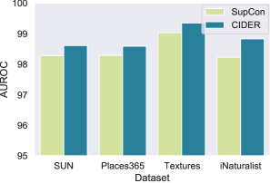
Figure 4: Fine-tuning pre-trained ResNet-34 on ImageNet-100 (ID).

4.4 Additional Ablations and Analysis

CIDER is competitive on large-scale datasets.

To further examine the performance of CIDER on real-world tasks, we evaluate the performance of CIDER on the more challenging large-scale benchmarks. Specifically, we use ImageNet-100 as ID, a subset of ImageNet (Deng et al., 2009) consisting of 100 randomly sampled classes. For OOD test datasets, we use the same ones in (Huang & Li, 2021), including subsets of iNaturalist (Van Horn et al., 2018), Sun (Xiao et al., 2010), Places (Zhou et al., 2017), and Texture (Cimpoi et al., 2014a). For each OOD dataset, the categories do not overlap with the ID dataset. For computational efficiency, we fine-tune pre-trained ResNet-34 with CIDER and SupCon losses for 10 epochs with an initial learning rate of 0.01. For each loss, we update the weights of the last residual block and the nonlinear projection head, while freezing the parameters in the first three residual blocks. At test time, we use the same detection score (KNN) to evaluate representation quality.

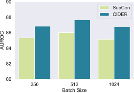
Figure 5: OOD Detection performance across different batch sizes.

The performance (in AUROC) is shown in Figure 4 (more results are in Appendix D). We can see that CIDER remains very competitive on all the OOD test sets where CIDER consistently outperforms SupCon. This further verifies the benefits of explicitly promoting inter-class dispersion and intra-class compactness.

Ablation studies on weight scale, prototype update factor, learning rate, temperature, batch size, and architecture. We provide comprehensive ablation studies to understand the impact of various factors in Appendix 8. For example, as shown in Figure 5, CIDER consistently outperforms SupCon across different batch sizes.

5 Related Works

Out-of-distribution detection. The majority of works in the OOD detection literature focus on the supervised setting, where the goal is to derive a binary ID-OOD classifier along with a classification model for the in-distribution data. Compared to generative model-based methods (Kirichenko et al., 2020; Nalisnick et al., 2019; Ren et al., 2019; Serrà et al., 2020; Xiao et al., 2020), OOD detection based on supervised discriminative models typically yield more competitive performance. For deep neural networks-based methods, most OOD detection methods derive confidence scores either based on the output (Bendale & Boult, 2016; Hendrycks & Gimpel, 2017; Hsu et al., 2020; Huang & Li, 2021; Liang et al., 2018; Liu et al., 2020; Sun et al., 2021; Ming et al., 2022b), gradient information (Huang et al., 2021), or the feature embeddings (Lee et al., 2018; Sastry & Oore, 2020; Tack et al., 2020; Zhou et al., 2021; Sehwag et al., 2021; Sun et al., 2022; Ming et al., 2022a; Du et al., 2022). Our method can be categorized as a distance-based OOD detection method by exploiting the hyperspherical embedding space.

Contrastive representation learning. Contrastive representation learning (van den Oord et al., 2019) aims to learn a discriminative embedding where positive samples are aligned while negative ones are dispersed. It has demonstrated remarkable success for visual representation learning in unsupervised (Chen et al., 2020a; b; He et al., 2020; Robinson et al., 2021), semi-supervised (Assran et al., 2021), and supervised settings (Khosla et al., 2020). Recently,  Li et al. (2021b) propose a prototype-based contrastive loss for unsupervised learning where prototypes are generated via a clustering algorithm, while our method is supervised where prototypes are updated based on labels.  Li et al. (2021a) incorporate a prototype-based loss to tackle data noise.  Wang & Isola (2020) analyze the asymptotic behavior of contrastive losses theoretically, while  Wang & Liu (2021a) empirically investigate the properties of contrastive losses for classification. Recently,  Bucci et al. (2022) investigates contrastive learning for open-set domain adaptation. However, none of the works focus on OOD detection. We aim to fill the gap and facilitate the design and understanding of contrastive losses for OOD detection.

Representation learning for OOD detection. Self-supervised learning has been shown to improve OOD detection. Prior works (Sehwag et al., 2021; Winkens et al., 2020) verify the effectiveness of directly applying the off-the-shelf multi-view contrastive losses such as SupCon and SimCLR for OOD detection. CSI (Tack et al., 2020) investigates the type of data augmentations that are particularly beneficial for OOD detection. Different from prior works, we focus on hyperspherical embeddings and propose to explicitly encourage the desirable properties for OOD detection, and thus alleviate the dependence on specific data augmentations or self-supervision. Moreover, CIDER explicitly models the latent representations as vMF distributions, providing a direct and clear geometrical interpretation of hyperspherical embeddings. Closest to our work,  Du et al. (2022) recently explores shaping representations into vMF distributions for object-level OOD detection. However, they do not consider the inter-class dispersion loss, which we show is crucial to achieve strong OOD detection performance.

Deep metric learning. Learning a desirable embedding is a fundamental goal in the deep metric learning community. Various losses have been proposed for face verification (Deng et al., 2019; Liu et al., 2017; Wang et al., 2018), person re-identification (Chen et al., 2017; Xiao et al., 2017), and image retrieval (Kim et al., 2019; Movshovitz-Attias et al., 2017; Oh Song et al., 2016; Teh et al., 2020). However, none of the works focus on desirable embeddings for OOD detection. The difference between CIDER and proxy-based methods has been discussed in Remark 2.

6 Conclusion and Outlook

In this work, we propose CIDER, a novel representation learning framework that exploits hyperspherical embeddings for OOD detection. CIDER jointly optimizes the dispersion and compactness losses to promote strong ID-OOD separability. We show that CIDER achieves superior performance on common OOD benchmarks, including large-scale OOD detection tasks. Moreover, we introduce new measurements to quantify the hyperspherical embedding, and establish the relationship with OOD detection performance. We conduct extensive ablations to understand the efficacy and behavior of CIDER under various settings and hyperparameters. We hope our work can inspire future methods of exploiting hyperspherical representations for OOD detection.

Appendix

Appendix A Algorithm Details and Discussions

The training scheme of our compactness and dispersion regularized (CIDER) learning framework is shown in Algorithm 1. We jointly optimize: (1) a compactness loss to encourage samples to be close to their class prototypes, and (2) a dispersion loss to encourage larger angular distances among different class prototypes.

1 Input: Training dataset $\mathcal{D}$, neural network encoder $f$, projection head $h$, classifier $g$, class prototypes $\bm{\mu}_{j}$ ($1\leq j\leq C$), weights of loss terms $\lambda_{d}$, and $\lambda_{c}$, temperature $\tau$

2 for $epoch=1,2,\ldots,$ do

3       for $iter=1,2,\ldots,$ do

4             sample a mini-batch $B=\{\mathbf{x}_{i},y_{i}\}_{i=1}^{b}$

5             obtain augmented batch $\tilde{B}=\{\tilde{\mathbf{x}}_{i},\tilde{y}_{i}\}_{i=1}^{2b}$ by applying two random augmentations to $\mathbf{x}_{i}\in B$ $\forall i\in\{1,2,\ldots,b\}$

6             for $\tilde{\mathbf{x}}_{i}\in\tilde{B}$ do

                   // obtain normalized embedding

7                   $\tilde{\mathbf{z}}_{i}=h(f(\tilde{\mathbf{x}}_{i}))$, $\mathbf{z}_{i}=\tilde{\mathbf{z}}_{i}/\lVert\tilde{\mathbf{z}}_{i}\rVert_{2}$

                   // update class-prototypes

8                   ${\bm{\mu}}_{c}:=\text{Normalize}(\alpha{\bm{\mu}}_{c}+(1-\alpha)\mathbf{z}_{i}),\;\forall c\in\{1,2,\ldots,C\}$

9                  

            // calculate compactness loss

10             $\mathcal{L}_{\mathrm{comp}}=-\sum_{i=1}^{b}\log\frac{\exp\left(\mathbf{z}_{i}^{\top}{\bm{\mu}}_{c(i)}/\tau\right)}{\sum_{j=1}^{C}\exp\left(\mathbf{z}_{i}^{\top}{\bm{\mu}}_{j}/\tau\right)}$

             // calculate dispersion loss

11             $\mathcal{L}_{\mathrm{dis}}={1\over C}\sum_{i=1}^{C}\log{1\over C-1}\sum_{j=1}^{C}\mathbbm{1}\{j\neq i\}e^{{\bm{\mu}}_{i}^{\top}{\bm{\mu}}_{j}/\tau}$

             // calculate overall loss

12             $\mathcal{L}=\mathcal{L}_{\mathrm{dis}}+\lambda_{c}\mathcal{L}_{\mathrm{comp}}$

             // update the network weights

13             update the weights in the encoder and the projection head

14            

15      

Algorithm 1 Pseudo-code of CIDER.

Remark 1: The prototype update rule. The class prototypes are only updated by exponential moving average (EMA). Since the prototypes are not learnable parameters, the gradients of the dispersion loss have no direct impact on their updates. EMA-style techniques have been used in prior works Li et al. (2020), and can be rigorously interpreted from a clustering-based Expectation-Maximization (EM) perspective. Alternatively, the prototypes can also be updated via gradients without EMA. We provide an ablation study of CIDER based on different prototype update rules in Appendix C.

Remark 2: CIDER vs. Wang & Isola (2020). The notion of alignment and uniformity for contrastive losses were proposed in Wang & Isola (2020) for the unsupervised setting where both metrics are based on individual samples. CIDER is a contrastive loss designed for the supervised setting. In particular, the uniform loss in Wang & Isola (2020) is defined based on randomly sampled pairs of data and promotes an instance-to-instance uniformity on the hypersphere. The notion of uniformity is fundamentally different from CIDER, which promotes prototype-to-prototype dispersion.

Remark 3: CIDER vs. Cross Entropy. When a model is trained with the cross-entropy (CE) loss, the weight matrix of the last fully connected layer can be interpreted as the set of class prototypes. However, CE is suboptimal for OOD detection for two main reasons: (1) CE does not explicitly optimize for the intra-class compactness and inter-class dispersion in the feature space. As a consequence, the embeddings obtained by CE loss display insufficient compactness and dispersion (Table 4). Compared to CE, CIDER is more structured by exploiting the hyperspherical embeddings and explicitly optimizing towards the desirable properties for OOD detection and ID classification. (2) the feature space obtained by CE loss is Euclidean instead of hyperspherical. As shown in Tack et al. (2020), ID data tend to have a larger norm than OOD data. As a result, the Euclidean distance between ID features can be larger than the distance from OOD to ID data. A recent work (Sun et al., 2022) verified that Euclidean embedding without feature normalization leads to suboptimal OOD detection performance. Instead, CIDER is designed to optimize hyperspherical embeddings, which benefit OOD detection.

Remark 4: On the measurement of embedding quality. In Section 4.3, we provide measurements of embedding quality (inter-class dispersion and intra-class compactness) via prototypes. In practice, one can replace the class prototypes in the dispersion and compactness metrics to be one random sample (or the average of a random subset) from the corresponding class. For example, on CIFAR-10, as the embeddings of CIDER are compact, we observe that the two metrics give similar results (e.g., the ID-OOD Separability is 42.5 with prototype-based metrics vs. 38.3 with instance-based metrics). We choose to use prototypes because (1) the definition directly maps to our loss function design, and (2) prototypes are calculated as the averaged feature for each class, which helps to mitigate the sampling bias.

Appendix B Experimental Details

Software and hardware. All methods are implemented in Pytorch 1.10. We run all the experiments on NVIDIA GeForce RTX-2080Ti GPU for small to medium batch size and on NVIDIA A100 GPU for large batch size and larger network encoder.

Architecture. As shown in Figure 1, the overall architecture of CIDER consists of a projection head $h$ on top of a deep neural network encoder $f$. Following common practice and fair comparison with prior works (Sehwag et al., 2021), (Khosla et al., 2020), we fix the output dimension of the projection head to be 128. We use a two-layer non-linear projection head for CIFAR-10 and CIFAR-100 as in  Sun et al. (2022).

Training. For methods based on pre-trained models such as MSP (Hendrycks & Gimpel, 2017), ODIN (Liang et al., 2018), Mahalanobis (Lee et al., 2018), and Energy (Liu et al., 2020), we follow the configurations in Sun et al. (2022) for CIFAR-10 and train with the cross-entropy loss for 100 epochs. The initial learning rate is $0.1$ and decays by a factor of 10 at epochs 50, 75, and 90 respectively. For the more challenging dataset CIFAR-100, we train 200 epochs. We use stochastic gradient descent with momentum $0.9$, and weight decay $10^{-4}$. For fair comparison, methods involving contrastive learning (Winkens et al., 2020),(Tack et al., 2020),(Sehwag et al., 2021) are trained for 500 epochs on CIFAR-10 and CIFAR-100. For CIDER, we adopt the same key hyperparameters for contrastive losses such as initial learning rate (0.5), temperature (0.1), and batch size (512) as SSD+ (Sehwag et al., 2021) in main experiments to demonstrate the effectiveness and simplicity of CIDER. For the prototype update factor $\alpha$, we set the default value as 0.95 for simplicity. We observed that $\alpha=0.95$ on CIFAR-10 with ResNet-18 and $\alpha=0.5$ on CIFAR-100 with ResNet-34 provide stronger performance.

OOD detection score. By default, we use the non-parametric KNN score Sun et al. (2022). We use a larger $K=300$ for CIFAR-100 and a smaller $K=100$ for CIFAR-10 for simplicity. Adjusting $K\in\{10,20,50,100,200,300,500\}$ yields similar performance. In practice, $K$ can be tuned using a validation method (Sun et al., 2022) to further improve the performance.

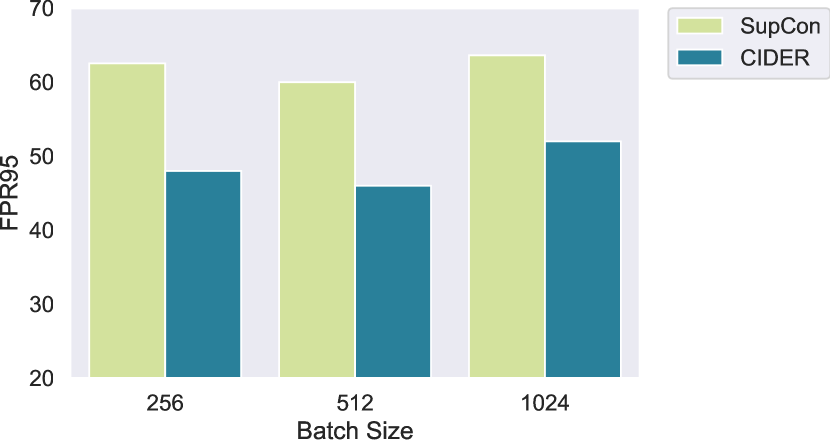
(a) FPR95 under different batch sizes

(b) AUROC under different batch sizes

Figure 6: Ablation on CIDER v.s. SupCon loss under different batch sizes. The results are averaged across the 5 OOD test sets based on ResNet-34. CIDER outperforms SupCon across different batch sizes, suggesting the effectiveness of explicitly facilitating prototype-wise dispersion.

Appendix C Additional Ablation Studies

CIDER is effective under various batch sizes.

Figure 6(a) and 6(b) also indicate that CIDER remains competitive under different batch size configurations compared to SupCon. To explain this, the standard SupCon loss requires instance-to-instance distance measurement, whereas compactness loss reduces the complexity to instance-to-prototype. The class-conditional prototypes are updated during training, which capture the average statistics of each class and alleviate the dependency on the batch size. This leads to an overall memory-efficient solution for OOD detection.

Ablation on the loss weights.

In the main results (Table 1), we demonstrate the effectiveness of CIDER where the loss weight $\lambda_{c}$ is simply set to balance the initial scale between the $\mathcal{L}_{\mathrm{dis}}$ and $\mathcal{L}_{\mathrm{comp}}$. In fact, CIDER can be further improved by adjusting $\lambda_{c}$. As shown in Figure 7(a), the performance of CIDER is relatively stable for moderate adjustments of $\lambda_{c}$ (e.g. 0.5 to 2), with the best performance at around $\lambda_{c}\in[1,2]$. This indicates CIDER provides a simple and effective solution for improving OOD detection, without much need for hyperparameter tuning on the loss scale.

Adjusting prototype update factor $\alpha$ improves CIDER. We show in Figure 7(b) the performance by varying the moving-average discount factor $\alpha$ in Eq. 8. We can observe that the detection performance (averaged over 5 test sets) is still competitive across a wide range of $\alpha$. In particular, for CIFAR-100, $\alpha=0.5$ results in the best performance with average FPR95 of $46.89\%$ under KNN score. For CIFAR-10, we observe that a larger $\alpha$ (e.g. 0.95 to 0.99) results in stronger performance.

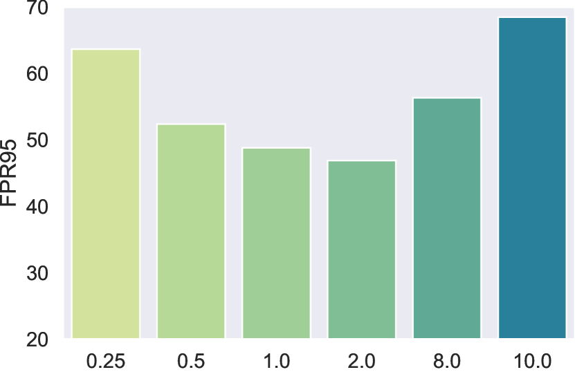
(a) weight $\lambda_{c}$

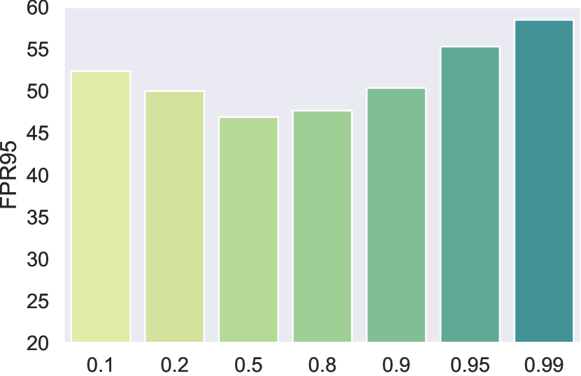
(b) Mov-avg $\alpha$

Figure 7: Ablation on (a) weight $\lambda_{c}$ of the compactness loss; (b) prototype update discount factor $\alpha$. The results are based on CIFAR-100 (ID) averaged over 5 OOD test sets.

Ablation on the learning rate. Prior works (Khosla et al., 2020; Sehwag et al., 2021) use a default initial learning rate (lr) of $0.5$ to train contrastive losses, which is also the default setting of CIDER. We further investigate the impact of the initial learning rate on OOD detection. As shown in Figure 8(a), a relatively higher initial lr is indeed desirable for competitive performance while too small lr (e.g. 0.1) would lead to performance degradation.

Small temperature $\tau$ leads to better performance. Figure 8(b) demonstrates the detection performance as we vary the temperature parameter $\tau$. We observe that the OOD detection performance is desirable at a relatively small temperature. Complementary to our finding, a relatively small temperature is shown to be desirable for ID classification (Khosla et al., 2020; Wang & Liu, 2021b) which penalizes hard negative samples with larger gradients and leads to separable features.

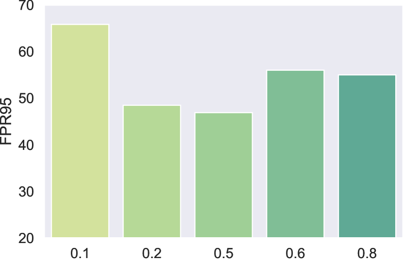
(a) init lr

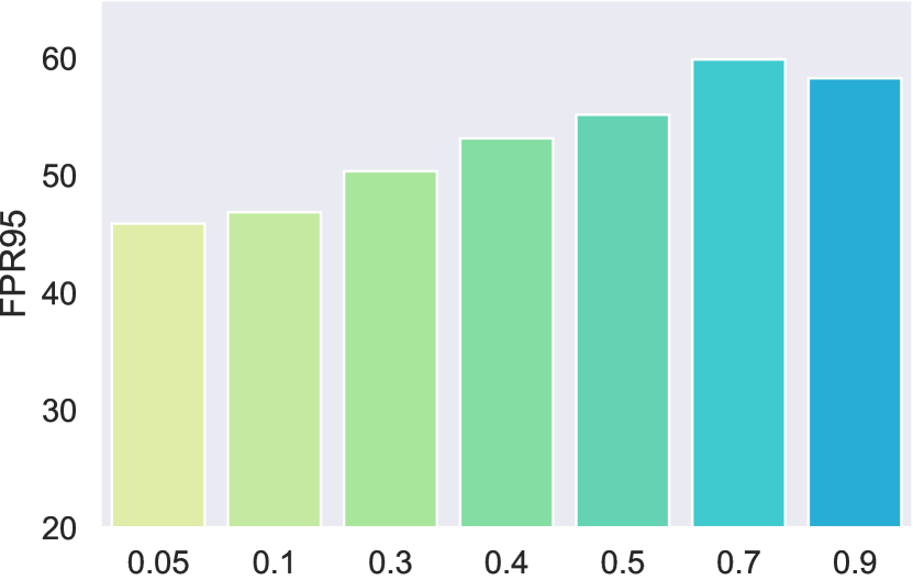
(b) temperature $\tau$

Figure 8: Ablation on (a) initial learning rate and (b) temperature. The results are based on CIFAR-100 (ID) averaged over 5 OOD test sets.

Ablation on network capacity.

We verify the effectiveness of CIDER under networks with other architectures such as ResNet-50 for CIFAR-100. The results are shown in Figure 9. The trend is similar to what we observed with ResNet-34. Specifically, as a result of the improved representation, training with CIDER improves the FPR95 for various test sets compared to training with the SupCon loss.

Ablation on gradient-based prototype update.

We examine the effect of updating prototypes via gradients. Compared to CIDER with EMA, CIDER with learnable prototypes (LP) can be more sensitive to initialization. We report the average performance of CIDER (EMA) and CIDER (LP) across 3 independent runs for CIFAR-10 in Table 5. All training and evaluation configurations (e.g., learning rate and batch size) are the same. We can see that CIDER with EMA improves the average FPR95 by $5.08\%$ with smaller standard deviation. Therefore, we empirically verify that updating prototypes via EMA is a better option with stronger training stability in practice.

Table 5: Ablation on prototype update rules. OOD detection performance for ResNet-18 trained on CIFAR-10 with EMA-style updates denoted as CIDER (EMA) vs. learnable prototypes denoted as CIDER (LP). CIDER with EMA demonstrates strong OOD detection performance. Results are averaged over 3 independent runs.

Method	OOD Dataset										Average
	SVHN		Places365		LSUN		iSUN		Texture
	FPR$\downarrow$	AUROC$\uparrow$	FPR$\downarrow$	AUROC$\uparrow$	FPR$\downarrow$	AUROC$\uparrow$	FPR$\downarrow$	AUROC$\uparrow$	FPR$\downarrow$	AUROC$\uparrow$	FPR$\downarrow$	AUROC$\uparrow$
CIDER (LP)	$2.17^{\pm 1.50}$	$99.55^{\pm 0.48}$	$28.13^{\pm 1.59}$	$94.53^{\pm 0.12}$	$5.23^{\pm 2.68}$	$98.16^{\pm 0.99}$	$36.47^{\pm 8.93}$	$94.59^{\pm 0.92}$	$16.25^{\pm 1.07}$	97.38 ±0.19	$17.65^{\pm 2.36}$	$96.84^{\pm 0.40}$
CIDER (EMA)	$3.04^{\pm 1.38}$	$99.50^{\pm{0.30}}$	$26.60^{\pm 2.47}$	$94.64^{\pm{0.51}}$	$4.10^{\pm 1.68}$	$99.14^{\pm{0.19}}$	$15.94^{\pm 4.56}$	$97.10^{\pm{0.54}}$	$13.19^{\pm 0.82}$	$97.39^{\pm{0.48}}$	$12.57^{\pm 1.31}$	$97.56^{\pm{0.33}}$

Stability of CIDER.

To verify that CIDER consistently provides strong performance, we train with 3 independent seeds for each ID dataset. Table 6 shows the OOD detection performance of CIDER with ResNet-18 trained on CIFAR-10 and ResNet-34 trained on CIFAR-100. Comparing Table 1 and Table 7, we can see that CIDER yields consistently strong performance. Code and checkpoints are provided in https://github.com/deeplearning-wisc/cider.

Table 6: Ablation on stability. OOD detection performance of CIDER for CIFAR-10 and CIFAR-100. Results are averaged over 3 independent runs.

ID Dataset	OOD Dataset										Average
	SVHN		Places365		LSUN		iSUN		Texture
	FPR$\downarrow$	AUROC$\uparrow$	FPR$\downarrow$	AUROC$\uparrow$	FPR$\downarrow$	AUROC$\uparrow$	FPR$\downarrow$	AUROC$\uparrow$	FPR$\downarrow$	AUROC$\uparrow$	FPR$\downarrow$	AUROC$\uparrow$
CIFAR-10	$3.04^{\pm 1.38}$	$99.50^{\pm{0.30}}$	$26.60^{\pm 2.47}$	$94.64^{\pm{0.51}}$	$4.10^{\pm 1.68}$	$99.14^{\pm{0.19}}$	$15.94^{\pm 4.56}$	$97.10^{\pm{0.54}}$	$13.19^{\pm 0.82}$	$97.39^{\pm{0.48}}$	$12.57^{\pm 1.31}$	$97.56^{\pm{0.33}}$
CIFAR-100	$23.67^{\pm{2.28}}$	$95.07^{\pm{0.13}}$	$79.37^{\pm{1.84}}$	$72.97^{\pm{3.90}}$	$22.04^{\pm{5.12}}$	$96.01^{\pm{1.80}}$	$62.16^{\pm{8.48}}$	$83.70^{\pm{2.92}}$	$44.96^{\pm{6.01}}$	$90.25^{\pm{0.97}}$	$46.45^{\pm{2.01}}$	$87.60^{\pm{1.03}}$

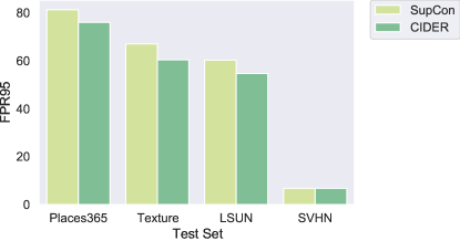
Figure 9: Ablation on architecture. Results are based on ResNet-50.

Appendix D Results on Large-scale Datasets

In recent years, there has been a paradigm shift towards fine-tuning pre-trained models, as opposed to training from scratch. Given this trend, it is important to explore whether CIDER remains effective based on pre-trained models. Specifically, we fine-tune ImageNet pre-trained ResNet-34 on ImageNet-100 with CIDER and SupCon losses for 10 epochs. For each loss, we update the weights of the last residual block and the nonlinear projection head, while freezing the parameters in the first three residual blocks. At test time, we use the same detection score (KNN) to evaluate representation quality. FPR95 and AUROC for each OOD test set are shown in Figure 10(a) and  10(b), respectively. The results suggest that CIDER remains very competitive, which highlight the benefits of promoting inter-class dispersion and intra-class compactness.

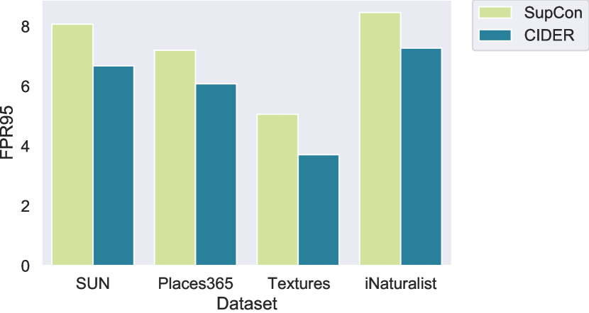
(a) FPR95 for different OOD test sets

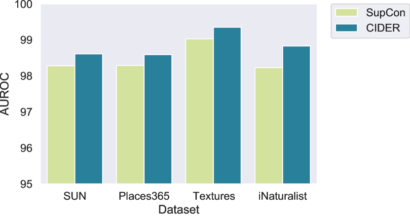
(b) AUROC for different OOD test sets

Figure 10: OOD detection performance of fine-tuning with CIDER v.s. SupCon for ImageNet-100 (ID). With the same detection score (KNN), CIDER consistently outperforms SupCon across all OOD test datasets.

Appendix E Results on CIFAR-10

In the main paper, we mainly focus on the more challenging task CIFAR-100. In this section, we additionally evaluate on CIFAR-10, a commonly used benchmark in literature. For methods involving contrastive losses, we use the same network encoder and embedding dimension, while only varying the training objective. The Mahalanobis score is used for OOD detection in SSD+ (Sehwag et al., 2021), CE+SimCLR (Winkens et al., 2020), SupCon, and CIDER. As CIFAR-10 is much less challenging compared to CIFAR-100, recent methods with contrastive losses yield similarly strong performance. For methods trained with cross-entropy loss, we use the publicly available checkpoints in  Sun et al. (2022) for better consistency. The results are shown in Table 7. Similar trends also hold as we describe in Section 4.2: (1) CIDER achieves superior OOD detection performance in CIFAR-10 as a result of better inter-class dispersion and intra-class compactness. For example, compared to the Mahalanobis baseline (Lee et al., 2018), CIDER reduces the FPR95 by $24.99\%$ averaged over 5 diverse test sets; (2) Although the ID classification accuracy of CIDER is similar to another proxy-based loss ProxyAnchor (Table 8), CIDER significantly improves the OOD detection performance by $21.05\%$ in FPR95 due to the addition of explicit inter-class dispersion which we show is critical for OOD detection in Section 4.3. The significant improvements highlight the importance of representation learning for OOD detection.

Method	OOD Dataset										Average
	SVHN		Places365		LSUN		iSUN		Texture
	FPR$\downarrow$	AUROC$\uparrow$	FPR$\downarrow$	AUROC$\uparrow$	FPR$\downarrow$	AUROC$\uparrow$	FPR$\downarrow$	AUROC$\uparrow$	FPR$\downarrow$	AUROC$\uparrow$	FPR$\downarrow$	AUROC$\uparrow$
	Without Contrastive Learning
MSP	59.66	91.25	62.46	88.64	45.21	93.80	54.57	92.12	66.45	88.50	57.67	90.86
Energy	54.41	91.22	42.77	91.02	10.19	98.05	27.52	95.59	55.23	89.37	38.02	93.05
ODIN	53.78	91.30	43.40	90.98	10.93	97.93	28.44	95.51	55.59	89.47	38.43	93.04
GODIN	18.72	96.10	55.25	85.50	11.52	97.12	30.02	94.02	33.58	92.20	29.82	92.97
Mahalanobis	9.24	97.80	83.50	69.56	67.73	73.61	6.02	98.63	23.21	92.91	37.94	86.50
	With Contrastive Learning
CE + SimCLR	6.98	99.22	54.39	86.70	64.53	85.60	59.62	86.78	16.77	96.56	40.46	90.97
CSI	37.38	94.69	38.31	93.04	10.63	97.93	10.36	98.01	28.85	94.87	25.11	95.71
SSD+	2.47	99.51	22.05	95.57	10.56	97.83	28.44	95.67	9.27	98.35	14.56	97.38
ProxyAnchor	39.27	94.55	43.46	92.06	21.04	97.02	23.53	96.56	42.70	93.16	34.00	94.67
KNN+	2.70	99.61	23.05	94.88	7.89	98.01	24.56	96.21	10.11	97.43	13.66	97.22
CIDER	2.89	99.72	23.88	94.09	5.45	99.01	20.21	96.64	12.33	96.85	12.95	97.26

Table 7: Results on CIFAR-10. OOD detection performance for ResNet-18 trained on CIFAR-10 with and without contrastive loss. CIDER achieves strong OOD detection performance and ID classification accuracy (Table 8).

Appendix F ID Classification Accuracy

The ID classification accuracy on CIFAR-10 and CIFAR-100 can be seen in Table 8 and Table 9, where for contrastive losses such as KNN+, SSD+, and CIDER, we follow the common practice as in Khosla et al. (2020) and use linear probe on normalized features.

Table 8: ID classification accuracy on CIFAR-10 (%)

Method	ID ACC
w.o. contrastive loss
MSP	94.21
ODIN	94.21
GODIN	93.64
Energy	94.21
Mahalanobis	94.21
w. contrastive loss
CE + SimCLR	93.12
SSD+	94.53
ProxyAnchor	94.21
KNN+	94.53
CIDER	94.58

Table 9: ID classification accuracy on CIFAR-100 (%)

Method	ID ACC
w.o. contrastive loss
MSP	74.59
ODIN	74.59
GODIN	74.92
Energy	74.59
Mahalanobis	74.59
w. contrastive loss
CE + SimCLR	73.54
SSD+	75.11
ProxyAnchor	74.21
KNN+	75.11
CIDER	75.35

References

- Assran et al. (2021) Mahmoud Assran, Mathilde Caron, Ishan Misra, Piotr Bojanowski, Armand Joulin, Nicolas Ballas, and Michael Rabbat. Semi-supervised learning of visual features by non-parametrically predicting view assignments with support samples. In Proceedings of the IEEE/CVF International Conference on Computer Vision (ICCV), pp. 8443–8452, 2021.
- Bendale & Boult (2016) Abhijit Bendale and Terrance E Boult. Towards open set deep networks. In CVPR, 2016.
- Bucci et al. (2022) Silvia Bucci, Francesco Cappio Borlino, Barbara Caputo, and Tatiana Tommasi. Distance-based hyperspherical classification for multi-source open-set domain adaptation. In Proceedings of the IEEE/CVF Winter Conference on Applications of Computer Vision, pp. 1119–1128, 2022.
- Chen et al. (2020a) Ting Chen, Simon Kornblith, Mohammad Norouzi, and Geoffrey Hinton. A simple framework for contrastive learning of visual representations. arXiv preprint arXiv:2002.05709, 2020a.
- Chen et al. (2017) Weihua Chen, Xiaotang Chen, Jianguo Zhang, and Kaiqi Huang. Beyond triplet loss: a deep quadruplet network for person re-identification. In Proceedings of the IEEE conference on computer vision and pattern recognition, pp. 403–412, 2017.
- Chen et al. (2020b) Xinlei Chen, Haoqi Fan, Ross Girshick, and Kaiming He. Improved baselines with momentum contrastive learning. arXiv preprint arXiv:2003.04297, 2020b.
- Cimpoi et al. (2014a) Mircea Cimpoi, Subhransu Maji, Iasonas Kokkinos, Sammy Mohamed, and Andrea Vedaldi. Describing textures in the wild. In Proceedings of the IEEE Conference on Computer Vision and Pattern Recognition, pp. 3606–3613, 2014a.
- Cimpoi et al. (2014b) Mircea Cimpoi, Subhransu Maji, Iasonas Kokkinos, Sammy Mohamed, and Andrea Vedaldi. Describing textures in the wild. In Proceedings of the IEEE Conference on Computer Vision and Pattern Recognition, pp. 3606–3613, 2014b.
- Deng et al. (2009) Jia Deng, Wei Dong, Richard Socher, Li-Jia Li, Kai Li, and Li Fei-Fei. Imagenet: A large-scale hierarchical image database. In 2009 IEEE conference on computer vision and pattern recognition, pp. 248–255. Ieee, 2009.
- Deng et al. (2019) Jiankang Deng, Jia Guo, Niannan Xue, and Stefanos Zafeiriou. Arcface: Additive angular margin loss for deep face recognition. In Proceedings of the IEEE/CVF conference on computer vision and pattern recognition, pp. 4690–4699, 2019.
- Du et al. (2022) Xuefeng Du, Gabriel Gozum, Yifei Ming, and Yixuan Li. Siren: Shaping representations for detecting out-of-distribution objects. In Advances in Neural Information Processing Systems, 2022.
- He et al. (2020) Kaiming He, Haoqi Fan, Yuxin Wu, Saining Xie, and Ross Girshick. Momentum contrast for unsupervised visual representation learning. In 2020 IEEE/CVF Conference on Computer Vision and Pattern Recognition (CVPR), pp. 9726–9735, 2020.
- Hendrycks & Gimpel (2017) Dan Hendrycks and Kevin Gimpel. A baseline for detecting misclassified and out-of-distribution examples in neural networks. In 5th International Conference on Learning Representations, ICLR 2017, 2017.
- Hsu et al. (2020) Yen-Chang Hsu, Yilin Shen, Hongxia Jin, and Zsolt Kira. Generalized odin: Detecting out-of-distribution image without learning from out-of-distribution data. In Proceedings of the IEEE/CVF Conference on Computer Vision and Pattern Recognition, pp. 10951–10960, 2020.
- Huang & Li (2021) Rui Huang and Yixuan Li. Towards scaling out-of-distribution detection for large semantic space. Proceedings of the IEEE/CVF Conference on Computer Vision and Pattern Recognition, 2021.
- Huang et al. (2021) Rui Huang, Andrew Geng, and Yixuan Li. On the importance of gradients for detecting distributional shifts in the wild. In Advances in Neural Information Processing Systems, 2021.
- Khosla et al. (2020) Prannay Khosla, Piotr Teterwak, Chen Wang, Aaron Sarna, Yonglong Tian, Phillip Isola, Aaron Maschinot, Ce Liu, and Dilip Krishnan. Supervised contrastive learning. In Advances in Neural Information Processing Systems, volume 33, pp. 18661–18673, 2020.
- Kim et al. (2019) Sungyeon Kim, Minkyo Seo, Ivan Laptev, Minsu Cho, and Suha Kwak. Deep metric learning beyond binary supervision. In Proceedings of the IEEE/CVF Conference on Computer Vision and Pattern Recognition, pp. 2288–2297, 2019.
- Kim et al. (2020) Sungyeon Kim, Dongwon Kim, Minsu Cho, and Suha Kwak. Proxy anchor loss for deep metric learning. In IEEE/CVF Conference on Computer Vision and Pattern Recognition (CVPR), 2020.
- Kirichenko et al. (2020) Polina Kirichenko, Pavel Izmailov, and Andrew G Wilson. Why normalizing flows fail to detect out-of-distribution data. Advances in Neural Information Processing Systems, 33, 2020.
- Krizhevsky et al. (2009) Alex Krizhevsky, Geoffrey Hinton, et al. Learning multiple layers of features from tiny images. 2009.
- Lee et al. (2018) Kimin Lee, Kibok Lee, Honglak Lee, and Jinwoo Shin. A simple unified framework for detecting out-of-distribution samples and adversarial attacks. In Advances in Neural Information Processing Systems, pp. 7167–7177, 2018.
- Li et al. (2020) Junnan Li, Caiming Xiong, and Steven Hoi. Mopro: Webly supervised learning with momentum prototypes. In International Conference on Learning Representations, 2020.
- Li et al. (2021a) Junnan Li, Caiming Xiong, and Steven C.H. Hoi. Learning from noisy data with robust representation learning. In Proceedings of the IEEE/CVF International Conference on Computer Vision (ICCV), pp. 9485–9494, 2021a.
- Li et al. (2021b) Junnan Li, Pan Zhou, Caiming Xiong, and Steven C.H. Hoi. Prototypical contrastive learning of unsupervised representations. In ICLR, 2021b.
- Liang et al. (2018) Shiyu Liang, Yixuan Li, and R. Srikant. Enhancing the reliability of out-of-distribution image detection in neural networks. In 6th International Conference on Learning Representations, ICLR 2018, 2018.
- Liu et al. (2020) Weitang Liu, Xiaoyun Wang, John Owens, and Yixuan Li. Energy-based out-of-distribution detection. Advances in Neural Information Processing Systems, 2020.
- Liu et al. (2017) Weiyang Liu, Yandong Wen, Zhiding Yu, Ming Li, Bhiksha Raj, and Le Song. Sphereface: Deep hypersphere embedding for face recognition. In The IEEE Conference on Computer Vision and Pattern Recognition (CVPR), 2017.
- Mardia et al. (2000) Kanti V Mardia, Peter E Jupp, and KV Mardia. Directional statistics, volume 2. Wiley Online Library, 2000.
- McInnes et al. (2018) Leland McInnes, John Healy, Nathaniel Saul, and Lukas Grossberger. Umap: Uniform manifold approximation and projection. The Journal of Open Source Software, 3(29):861, 2018.
- Ming et al. (2022a) Yifei Ming, Ziyang Cai, Jiuxiang Gu, Yiyou Sun, Wei Li, and Yixuan Li. Delving into out-of-distribution detection with vision-language representations. In Advances in Neural Information Processing Systems, 2022a.
- Ming et al. (2022b) Yifei Ming, Ying Fan, and Yixuan Li. POEM: Out-of-distribution detection with posterior sampling. In Proceedings of the 39th International Conference on Machine Learning, pp. 15650–15665, 2022b.
- Movshovitz-Attias et al. (2017) Yair Movshovitz-Attias, Alexander Toshev, Thomas K Leung, Sergey Ioffe, and Saurabh Singh. No fuss distance metric learning using proxies. In Proceedings of the IEEE International Conference on Computer Vision, pp. 360–368, 2017.
- Nalisnick et al. (2019) Eric Nalisnick, Akihiro Matsukawa, Yee Whye Teh, Dilan Gorur, and Balaji Lakshminarayanan. Do deep generative models know what they don’t know? In International Conference on Learning Representations, 2019.
- Netzer et al. (2011) Yuval Netzer, Tao Wang, Adam Coates, Alessandro Bissacco, Bo Wu, and Andrew Y Ng. Reading digits in natural images with unsupervised feature learning. 2011.
- Nguyen et al. (2015) Anh Nguyen, Jason Yosinski, and Jeff Clune. Deep neural networks are easily fooled: High confidence predictions for unrecognizable images. In Proceedings of the IEEE conference on computer vision and pattern recognition, pp. 427–436, 2015.
- Oh Song et al. (2016) Hyun Oh Song, Yu Xiang, Stefanie Jegelka, and Silvio Savarese. Deep metric learning via lifted structured feature embedding. In Proceedings of the IEEE conference on computer vision and pattern recognition, pp. 4004–4012, 2016.
- Ren et al. (2019) Jie Ren, Peter J Liu, Emily Fertig, Jasper Snoek, Ryan Poplin, Mark Depristo, Joshua Dillon, and Balaji Lakshminarayanan. Likelihood ratios for out-of-distribution detection. In Advances in Neural Information Processing Systems, pp. 14680–14691, 2019.
- Robinson et al. (2021) Joshua David Robinson, Ching-Yao Chuang, Suvrit Sra, and Stefanie Jegelka. Contrastive learning with hard negative samples. In International Conference on Learning Representations, 2021.
- Sastry & Oore (2020) Chandramouli Shama Sastry and Sageev Oore. Detecting out-of-distribution examples with Gram matrices. In Proceedings of the 37th International Conference on Machine Learning. PMLR, 2020.
- Sehwag et al. (2021) Vikash Sehwag, Mung Chiang, and Prateek Mittal. Ssd: A unified framework for self-supervised outlier detection. In International Conference on Learning Representations, 2021.
- Serrà et al. (2020) Joan Serrà, David Álvarez, Vicenç Gómez, Olga Slizovskaia, José F. Núñez, and Jordi Luque. Input complexity and out-of-distribution detection with likelihood-based generative models. In International Conference on Learning Representations, 2020.
- Sun et al. (2021) Yiyou Sun, Chuan Guo, and Yixuan Li. React: Out-of-distribution detection with rectified activations. In Advances in Neural Information Processing Systems, 2021.
- Sun et al. (2022) Yiyou Sun, Yifei Ming, Xiaojin Zhu, and Yixuan Li. Out-of-distribution detection with deep nearest neighbors. ICML, 2022.
- Tack et al. (2020) Jihoon Tack, Sangwoo Mo, Jongheon Jeong, and Jinwoo Shin. Csi: Novelty detection via contrastive learning on distributionally shifted instances. In Advances in Neural Information Processing Systems, 2020.
- Teh et al. (2020) Eu Wern Teh, Terrance DeVries, and Graham W Taylor. Proxynca++: Revisiting and revitalizing proxy neighborhood component analysis. In European Conference on Computer Vision, pp. 448–464. Springer, 2020.
- van den Oord et al. (2019) Aaron van den Oord, Yazhe Li, and Oriol Vinyals. Representation learning with contrastive predictive coding, 2019.
- Van Horn et al. (2018) Grant Van Horn, Oisin Mac Aodha, Yang Song, Yin Cui, Chen Sun, Alex Shepard, Hartwig Adam, Pietro Perona, and Serge Belongie. The inaturalist species classification and detection dataset. In Proceedings of the IEEE conference on computer vision and pattern recognition, pp. 8769–8778, 2018.
- Wang & Liu (2021a) Feng Wang and Huaping Liu. Understanding the behaviour of contrastive loss. In Proceedings of the IEEE/CVF Conference on Computer Vision and Pattern Recognition (CVPR), pp. 2495–2504, 2021a.
- Wang & Liu (2021b) Feng Wang and Huaping Liu. Understanding the behaviour of contrastive loss. In Proceedings of the IEEE/CVF Conference on Computer Vision and Pattern Recognition (CVPR), pp. 2495–2504, 2021b.
- Wang et al. (2018) Hao Wang, Yitong Wang, Zheng Zhou, Xing Ji, Dihong Gong, Jingchao Zhou, Zhifeng Li, and Wei Liu. Cosface: Large margin cosine loss for deep face recognition. In Proceedings of the IEEE conference on computer vision and pattern recognition, pp. 5265–5274, 2018.
- Wang & Isola (2020) Tongzhou Wang and Phillip Isola. Understanding contrastive representation learning through alignment and uniformity on the hypersphere. In International Conference on Machine Learning, pp. 9929–9939. PMLR, 2020.
- Wei et al. (2022) Hongxin Wei, Renchunzi Xie, Hao Cheng, Lei Feng, Bo An, and Yixuan Li. Mitigating neural network overconfidence with logit normalization. 2022.
- Winkens et al. (2020) Jim Winkens, Rudy Bunel, Abhijit Guha Roy, Robert Stanforth, Vivek Natarajan, Joseph R Ledsam, Patricia MacWilliams, Pushmeet Kohli, Alan Karthikesalingam, Simon Kohl, et al. Contrastive training for improved out-of-distribution detection. arXiv preprint arXiv:2007.05566, 2020.
- Xiao et al. (2010) Jianxiong Xiao, James Hays, Krista A Ehinger, Aude Oliva, and Antonio Torralba. Sun database: Large-scale scene recognition from abbey to zoo. In 2010 IEEE computer society conference on computer vision and pattern recognition (CVPR), pp. 3485–3492. IEEE, 2010.
- Xiao et al. (2017) Tong Xiao, Shuang Li, Bochao Wang, Liang Lin, and Xiaogang Wang. Joint detection and identification feature learning for person search. In Proceedings of the IEEE conference on computer vision and pattern recognition, pp. 3415–3424, 2017.
- Xiao et al. (2020) Zhisheng Xiao, Qing Yan, and Yali Amit. Likelihood regret: An out-of-distribution detection score for variational auto-encoder. Advances in Neural Information Processing Systems, 33, 2020.
- Xing et al. (2020) Chen Xing, Sercan Arik, Zizhao Zhang, and Tomas Pfister. Distance-based learning from errors for confidence calibration. In International Conference on Learning Representations, 2020.
- Xu et al. (2015) Pingmei Xu, Krista A Ehinger, Yinda Zhang, Adam Finkelstein, Sanjeev R Kulkarni, and Jianxiong Xiao. Turkergaze: Crowdsourcing saliency with webcam based eye tracking. arXiv preprint arXiv:1504.06755, 2015.
- Yu et al. (2015) Fisher Yu, Ari Seff, Yinda Zhang, Shuran Song, Thomas Funkhouser, and Jianxiong Xiao. Lsun: Construction of a large-scale image dataset using deep learning with humans in the loop. arXiv preprint arXiv:1506.03365, 2015.
- Zhou et al. (2017) Bolei Zhou, Agata Lapedriza, Aditya Khosla, Aude Oliva, and Antonio Torralba. Places: A 10 million image database for scene recognition. IEEE transactions on pattern analysis and machine intelligence, 40(6):1452–1464, 2017.
- Zhou et al. (2021) Zhi Zhou, Lan-Zhe Guo, Zhanzhan Cheng, Yu-Feng Li, and Shiliang Pu. Step: Out-of-distribution detection in the presence of limited in-distribution labeled data. In Advances in Neural Information Processing Systems, 2021.