Abstract

Flavor violating processes in the lepton sector have highly suppressed branching ratios in the standard model. Thus, observation of lepton flavor violation (LFV) constitutes a clear indication of physics beyond the standard model (BSM). We review new physics searches in the processes that violate the conservation of lepton (muon) flavor by two units with muonia and muonium–antimuonium oscillations.

8 1 169 Academic Editor: Bertrand Echenard and Robert H. Bernstein 20 December 2021 4 March 2022 8 March 2022 https://doi.org/
10.3390/universe8030169 Studying $\Delta L=2$ Lepton Flavor Violation with Muons Studying $\Delta L=2$ Lepton Flavor Violation with Muons Alexey A. Petrov ^1,2,3,*, Renae Conlin ¹ and Cody Grant ¹ Alexey A. Petrov, Renae Conlin and Cody Grant Petrov, A.A.; Conlin, R.; Grant, C. Correspondence: apetrov@wayne.edu

1 Introduction

Flavor-changing neutral current (FCNC) interactions serve as a powerful probe of physics beyond the standard model (BSM). Since no local operators generate FCNCs in the standard model (SM) at tree level, new physics (NP) degrees of freedom can effectively compete with the SM particles running in the loop graphs, making their discovery possible. This is, of course, only true provided the BSM models include flavor-violating interactions. If the new physics particles are heavier than the muon mass, their effect on muon transitions can be parameterized in terms of local operators of increasing dimension. In fact, any new physics scenario which involves lepton flavor violating interactions can be matched to an effective Lagrangian of the Standard Model Effective Field Theory (SM EFT),

$${\cal L}_{\rm SMEFT}=-\frac{1}{\Lambda^{2}}\underset{i}{\sum}c_{i}(\mu)Q_{i},$$ (1)

where the Wilson coefficients (WC) $c_{i}$ of ${\cal L}_{\rm SMEFT}$ in Equation (1) are determined by the UV physics that becomes active at some scale $\Lambda$ Petrov:2021idw ; Grzadkowski:2010es ; Petrov:2016azi .

The effective operators $Q_{i}$’s defined in Equation (1) reflect degrees of freedom relevant at the scale at which a given process takes place. For heavy new physics scenarios, those operators should be written in terms of muon, electron, neutrino, or photon (gluon) fields. Then to perform low energy computations, it is often convenient to match the SM EFT Lagrangian to the low energy Lagrangian ${\cal L}_{\rm eff}$ only containing these degrees of freedom. In addition, it is convenient to classify the operators of ${\cal L}_{\rm eff}$ by their lepton quantum numbers $L_{\ell}$ (with $\ell=e,\mu,\tau$),

$${\cal L}_{\rm eff}={\cal L}_{\rm eff}^{\Delta L_{\mu}=0}+{\cal L}_{\rm eff}^{\Delta L_{\mu}=1}+{\cal L}_{\rm eff}^{\Delta L_{\mu}=2}$$ (2)

We shall employ the operators that only contain the fermion fields, so the operators in Equation (2) start at dimension six.

The first term in Equation (2) contains both the standard model and the new physics contributions. The SM piece is given by the usual Fermi Lagrangian,

$${\cal L}_{\rm eff}^{\Delta L_{\mu}=0}=-\frac{4G_{F}}{\sqrt{2}}\left(\overline{\mu}_{L}\gamma_{\alpha}e_{L}\right)\left(\overline{\nu_{e}}_{L}\gamma^{\alpha}{\nu_{\mu}}_{L}\right).$$ (3)

Since $\Lambda\gg m_{W}$, which is required for the consistency of SM EFT, we can neglect the NP piece of the $\Delta L_{\mu}=0$ Lagrangian for studies of FCNC transitions. This implies that ${\cal L}_{\rm eff}^{\Delta L_{\mu}=0}$ is suppressed by powers of $G_{F}\sim M_{W}^{-2}$, the Fermi constant. We should emphasize that only the operators that are local at the scale of the muonium mass are retained in Equation (2).

The second term in Equation (2) contains $\Delta L_{\mu}=1$ operators. The most general low energy Lagrangian representing muon flavor change by one unit, $\mathcal{L}_{\rm eff}^{\Delta L_{\mu}=1}$, is conventionnaly written as Celis:2014asa ; Hazard:2017udp ; Hazard:2016fnc

$${\cal L}_{\rm eff}^{\Delta L_{\mu}=1}= - \frac{1}{\Lambda^{2}}\sum_{f}\Big{[}\left(C_{VR}^{f}\ \overline{\mu}_{R}\gamma^{\alpha}e_{R}+C_{VL}^{f}\ \overline{\mu}_{L}\gamma^{\alpha}e_{L}\right)\ \overline{f}\gamma_{\alpha}f$$

$$+ \ \left(C_{AR}^{f}\ \overline{\mu}_{R}\gamma^{\alpha}e_{R}+C_{AL}^{q}\ \overline{\mu}_{L}\gamma^{\alpha}e_{L}\right)\ \overline{f}\gamma_{\alpha}\gamma_{5}f$$

$$+ \ m_{e}m_{f}G_{F}\left(C_{SR}^{f}\ \overline{\mu}_{R}e_{L}+C_{SL}^{f}\ \overline{\mu}_{L}e_{R}\right)\ \overline{f}f$$

$$+ \ m_{e}m_{f}G_{F}\left(C_{PR}^{f}\ \overline{\mu}_{R}e_{L}+C_{PL}^{f}\ \overline{\mu}_{L}e_{R}\right)\ \overline{f}\gamma_{5}f$$

$$+ \ m_{e}m_{f}G_{F}\left(C_{TR}^{f}\ \overline{\mu}_{R}\sigma^{\alpha\beta}e_{L}+C_{TL}^{f}\ \overline{\mu}_{L}\sigma^{\alpha\beta}e_{R}\right)\ \overline{f}\sigma_{\alpha\beta}f+h.c.\Big{]},$$

where $\mu$ and $e$ are the fermion fields with $(\mu,e)_{L,R}=P_{L,R}(\mu,e)$, where $P_{R,L}=\frac{1}{2}\left(1\pm\gamma^{5}\right)$ are the projection operators, and $f$ represents other fermions that are not integrated out from the low energy effective theory. We introduced indices for the Wilson coefficients $C_{IK}^{f}$ to indicate the Lorentz structure of effective operators: vector, axial-vector, scalar, pseudo-scalar, and tensor. The Wilson coefficients are in general different for different fermions $f$. The operators additionally suppressed by factors of $m_{i}m_{j}G_{F}$ usually arise from SM EFT operators of dimension higher than six Celis:2014asa ; Hazard:2017udp .

The last term in the low energy EFT described in Equation (2), ${\cal L}_{\rm eff}^{\Delta L_{\mu}=2}$, represents a collection of effective operators changing the lepton quantum number by two units. The most general effective Lagrangian for such transition that is applicable to the physics we will discuss in this review is given by

$${\cal L}_{\rm eff}^{\Delta L_{\mu}=2}=-\frac{1}{\Lambda^{2}}\underset{i}{\sum}C^{\Delta L=2}_{i}(\mu)Q_{i}(\mu).$$ (5)

with the operators written entirely in terms of the muon and electron degrees of freedom,

$$Q_{1} = \left(\overline{\mu}_{L}\gamma_{\alpha}e_{L}\right)\left(\overline{\mu}_{L}\gamma^{\alpha}e_{L}\right),\quad Q_{2}=\left(\overline{\mu}_{R}\gamma_{\alpha}e_{R}\right)\left(\overline{\mu}_{R}\gamma^{\alpha}e_{R}\right),$$

$$Q_{3} = \left(\overline{\mu}_{L}\gamma_{\alpha}e_{L}\right)\left(\overline{\mu}_{R}\gamma^{\alpha}e_{R}\right),\quad Q_{4}=\left(\overline{\mu}_{L}e_{R}\right)\left(\overline{\mu}_{L}e_{R}\right),$$

$$Q_{5} = \left(\overline{\mu}_{R}e_{L}\right)\left(\overline{\mu}_{R}e_{L}\right).$$ (6)

Other Lorentz structures of the operators could be related to the ones in Equation (1) via Fierz relations. A $\Delta L=2$ interaction described by this Lagrangian can lead to muon decays such as $\mu^{+}\to 3e$. It can also change a $\mu^{+}e^{-}$ bound state into a $\mu^{-}e^{+}$ bound state, leading to muonium–antimuonium oscillations. We will discuss those below.

In addition, the operators built out of muon and electron fields, we can construct other $\Delta L_{\mu}=2$ local operators that contain muon, electron, and neutrino fields Conlin:2020veq ,

$$Q_{6}=\left(\overline{\mu}_{L}\gamma_{\alpha}e_{L}\right)\left(\overline{\nu_{\mu}}_{L}\gamma^{\alpha}{\nu_{e}}_{L}\right),\quad Q_{7}=\left(\overline{\mu}_{R}\gamma_{\alpha}e_{R}\right)\left(\overline{\nu_{\mu}}_{L}\gamma^{\alpha}{\nu_{e}}_{L}\right),$$ (7)

where we only included operators that contain left-handed neutrinos Petrov:2016azi ; Grossman:2003rw . The operators in Equation (7) could lead to both muon decays $\mu\to e\nu_{\mu}\bar{\nu}_{e}$ (note the “reversed" neutrino flavors), and muonium–antimuonium oscillations.

The goal of experimental studies of $\Delta L=2$ transitions would be to find the observables that are sensitive to various combinations of Wilson coefficients of the effective Lagrangian in Equation (2). Different processes are in general sensitive to different combinations of the Wilson coefficients, which raises hope that a sufficient number of measurements would allow placing constraints on individual WCs without additional assumptions such as single operator dominance Hazard:2016fnc ; Hazard:2017udp . In that respect, studies of both unbound muon and muonium decays are needed.

2 Muonium: The Simplest Bound State

Even though the hydrogen atom is a quintessential quantum-mechanical bound state and is usually presented as the easiest QED problem, it is not the simplest. Precision studies of hydrogen reveal effects related to the structure of the proton: its finite size and composite nature. In that respect, the simplest hydrogen-like system is built entirely out of leptons. Such a system that is especially clean for studies of BSM effects in the lepton sector is muonium ${M_{\mu}}$. The muonium is a QED bound state of a positively-charged muon and a negatively-charged electron, $|{M_{\mu}}\rangle\equiv|\mu^{+}e^{-}\rangle$.

Since muon is unstable, ${M_{\mu}}$ is unstable. The main decay channel for the muonium is determined by the weak decay of the muon, ${M_{\mu}}\to e^{+}e^{-}\bar{\nu}_{\mu}\nu_{e}$, so the average lifetime of a muonium state $\tau_{M_{\mu}}$ is expected to be the same as that of the muon,

$$1/\tau_{M_{\mu}}=\Gamma\left({M_{\mu}}\to e^{+}e^{-}\nu_{e}\bar{\nu}_{\mu}\right)\approx\Gamma\left(\mu\to e^{+}\nu_{e}\bar{\nu}_{\mu}\right)=\frac{G_{F}^{2}m_{\mu}^{5}}{192\pi^{3}}=1/\tau_{\mu},$$ (8)

with $\tau_{\mu}=(2.1969811\pm 0.0000022)\times 10^{-6}$ s Tanabashi:2018oca , apart from the tiny effect due to time dilation Czarnecki:1999yj . Note that Equation (8) represents the leading-order result. The results including subleading corrections are available Czarnecki:1999yj .

Like a hydrogen atom, muonium could be formed in two spin configurations. A spin-one triplet state $\left|{M_{\mu}^{V}}\right\rangle$ is called ortho-muonium, while a spin-zero singlet state $\left|{M_{\mu}^{P}}\right\rangle$ called para-muonium. In what follows, we will drop the superscript and employ the notation $\left|{M_{\mu}}\right\rangle$ if the spin of the muonium state is not important for the discussion.

3 Muonium–Antimuonium Oscillations

Since $\Delta L=2$ interaction can change the muonium state into the anti-muonium one, the possibility to study muonium–anti-muonium oscillations arises. Theoretical analyses of conversion probability for muonium into antimuonium have been performed, both in particular new physics models Pontecorvo:1957cp ; Feinberg:1961zza ; ClarkLove:2004 ; CDKK:2005 ; Li:2019xvv ; Endo:2020mev , and using the framework of effective theory Conlin:2020veq , where all possible BSM models are encoded in a few Wilson coefficients of effective operators. Observation of muonium converting into anti-muonium provides clean probes of new physics in the leptonic sector Bernstein:2013hba ; Willmann:1998gd .

3.1 Phenomenology of Muonium Oscillations

In order to determine experimental observables related to $M_{\mu}-\overline{M}_{\mu}$ oscillations, we recall that the treatment of the two-level system that represents muonium and antimuonium is similar to that of meson-antimeson oscillations Petrov:2021idw ; Donoghue ; Nierste . There are, however, several important differences. First, both ortho- and para-muonium can oscillate. Second, the SM oscillation probability is tiny, as it is related to a function of neutrino masses, so any experimental indication of oscillation would represent a sign of new physics.

In the presence of the interactions coupling ${M_{\mu}}$ and ${\overline{M}_{\mu}}$, the time development of a muonium and anti-muonium states would be coupled, so it would be appropriate to consider their combined evolution,

$$|\psi(t)\rangle=\left({\begin{array}[]{c}a(t)\\ b(t)\\ \end{array}}\right)=a(t)|{M_{\mu}}\rangle+b(t)|{\overline{M}_{\mu}}\rangle.$$ (9)

The time evolution of $|\psi(t)\rangle$ evolution is governed by a Schrödinger-like equation,

$$i\frac{d}{dt}\begin{pmatrix}\left|M_{\mu}(t)\right\rangle\\ \left|\overline{M}_{\mu}(t)\right\rangle\end{pmatrix}=\left(m-i\frac{\Gamma}{2}\right)\begin{pmatrix}\left|M_{\mu}(t)\right\rangle\\ \left|\overline{M}_{\mu}(t)\right\rangle\end{pmatrix}.$$ (10)

where $\left(m-i\frac{\Gamma}{2}\right)_{ik}$ is a $2\times 2$ Hamiltonian (mass matrix) with non-zero off-diagonal terms originating from the $\Delta L=2$ interactions. CPT-invariance dictates that the masses and widths of the muonium and anti-muonium are the same, so $m_{11}=m_{22}$, $\Gamma_{11}=\Gamma_{22}$. In what follows, we assume CP-invariance of the $\Delta L_{\mu}=2$ interactionA more general formalism without this assumption follows the same steps as that for the $B\bar{B}$ or $K\bar{K}$ mixing Petrov:2021idw ; Donoghue .. Then,

$$m_{12}=m^{*}_{21},\qquad\Gamma_{12}=\Gamma^{*}_{21}.$$ (11)

The off-diagonal matrix elements in Equation (11) can be related to the matrix elements of the effective operators introduced in Section 1, as discussed in Petrov:2021idw ; Donoghue ,

$$\left(m-\frac{i}{2}\Gamma\right)_{12}=\frac{1}{2M_{M}}\left\langle{\overline{M}_{\mu}}\left|{\cal H}_{\rm eff}\right|{M_{\mu}}\right\rangle+\frac{1}{2M_{M}}\sum_{n}\frac{\left\langle{\overline{M}_{\mu}}\left|{\cal H}_{\rm eff}\right|n\right\rangle\left\langle n\left|{\cal H}_{\rm eff}\right|{M_{\mu}}\right\rangle}{M_{M}-E_{n}+i\epsilon}.$$ (12)

To find the propagating states, the mass matrix needs to be diagonalized. The basis in which the mass matrix is diagonal is represented by the mass eigenstates $|{M_{\mu}}_{1,2}\rangle$, which are related to the flavor eigenstates ${M_{\mu}}$ and ${\overline{M}_{\mu}}$ as

$$|{M_{\mu}}_{1,2}\rangle=\frac{1}{\sqrt{2}}\left[|{M_{\mu}}\rangle\mp|{\overline{M}_{\mu}}\rangle\right],$$ (13)

where we employed a convention where $CP|{M_{\mu}}_{\pm}\rangle=\mp|{M_{\mu}}_{\pm}\rangle$. The mass and the width differences of the mass eigenstates are

$$\Delta m\equiv M_{1}-M_{2},\qquad\Delta\Gamma\equiv\Gamma_{2}-\Gamma_{1}.$$ (14)

Here, $M_{i}$ ($\Gamma_{i}$) are the masses (widths) of the physical mass eigenstates $|{M_{\mu}}_{1,2}\rangle$.

It is interesting to see how the Equation (12) defines the mass and the lifetime differences. Since the first term in Equation (12) is defined by a local operator, its matrix element does not develop an absorptive part, so it contributes to $m_{12}$, i.e., the mass difference. The second term contains bi-local contributions connected by physical intermediate states. This term has both real and imaginary parts and thus contributes to both $m_{12}$ and $\Gamma_{12}$.

It is often convenient to introduce dimensionless quantities,

$$x=\frac{\Delta m}{\Gamma},\qquad y=\frac{\Delta\Gamma}{2\Gamma},$$ (15)

where the average lifetime $\Gamma=(\Gamma_{1}+\Gamma_{2})/2$, and $M_{M}=\left(M_{1}+M_{2}\right)/2$ is the muonium mass. Noting that $\Gamma$ is defined by the standard model decay rate of the muon, and $x$ and $y$ are driven by the lepton-flavor violating interactions, we should expect that both $x,y\ll 1$.

The time evolution of flavor eigenstates follows from Equation (10) Donoghue ; Nierste ; Conlin:2020veq ,

$$\left|M(t)\right\rangle = g_{+}(t)\left|{M_{\mu}}\right\rangle+g_{-}(t)\left|{\overline{M}_{\mu}}\right\rangle,$$

$$\left|\overline{M}(t)\right\rangle = g_{-}(t)\left|{M_{\mu}}\right\rangle+g_{+}(t)\left|{\overline{M}_{\mu}}\right\rangle,$$ (16)

where the coefficients $g_{\pm}(t)$ are defined as

$$g_{\pm}(t)=\frac{1}{2}e^{-\Gamma_{1}t/2}e^{-iM_{1}t}\left[1\pm e^{\Delta\Gamma t/2}e^{i\Delta mt}\right].$$ (17)

As $x,y\ll 1$ we can expand Equation (17) in power series in $x$ and $y$ to obtain

$$g_{+}(t) = e^{-\Gamma_{1}t/2}e^{-iM_{1}t}\left[1+\frac{1}{8}\left(y-ix\right)^{2}\left(\Gamma t\right)^{2}\right],$$

$$g_{-}(t) = \frac{1}{2}e^{-\Gamma_{1}t/2}e^{-iM_{1}t}\left(y-ix\right)\left(\Gamma t\right).$$ (18)

The most natural way to detect $M_{\mu}-\overline{M}_{\mu}$ oscillations experimentally is by producing ${M_{\mu}}$ state and looking for the decay products of the CP-conjugated state ${\overline{M}_{\mu}}$. Denoting an amplitude for the ${M_{\mu}}$ decay into a final state $f$ as $A_{f}=\langle f|{\cal H}|{M_{\mu}}\rangle$ and an amplitude for its decay into a CP-conjugated final state $\overline{f}$ as $A_{\bar{f}}=\langle\overline{f}|{\cal H}|{M_{\mu}}\rangle$, we can write the time-dependent decay rate of ${M_{\mu}}$ into the $\overline{f}$,

$$\Gamma({M_{\mu}}\to\overline{f})(t)=\frac{1}{2}N_{f}\left|A_{f}\right|^{2}e^{-\Gamma t}\left(\Gamma t\right)^{2}R_{M}(x,y),$$ (19)

where $N_{f}$ is a phase-space factor and we defined the oscillation rate $R_{M}(x,y)$ as

$$R_{M}(x,y)=\frac{1}{2}\left(x^{2}+y^{2}\right).$$ (20)

Integrating over time and normalizing to $\Gamma({M_{\mu}}\to f)$ we get the probability of ${M_{\mu}}$ decaying as ${\overline{M}_{\mu}}$ at some time $t>0$,

$$P({M_{\mu}}\rightarrow{\overline{M}_{\mu}})=\frac{\Gamma({M_{\mu}}\to\overline{f})}{\Gamma({M_{\mu}}\to f)}=R_{M}(x,y).$$ (21)

The equation Equation (21) Conlin:2020veq generalizes oscillation probability found in the papers Feinberg:1961zza ; CDKK:2005 by allowing for a non-zero lifetime difference in $M_{\mu}-\overline{M}_{\mu}$ oscillations. We will review how $x$ and $y$ are related to the fundamental parameters of the Lagrangian below Conlin:2020veq .

3.2 The Mass Difference $x$

The physical mixing parameters $x$ and $y$ can be obtained from Equation (15). The mass difference $x$ comes from the dispersive part of the correlator.

$$x=\frac{1}{2M_{M}\Gamma}\mbox{Re}\left[2\langle{\overline{M}_{\mu}}\left|{\cal H}_{\rm eff}\right|{M_{\mu}}\rangle+\langle{\overline{M}_{\mu}}\left|i\int d^{4}x\ \mbox{T}\left[{\cal H}_{\rm eff}(x){\cal H}_{\rm eff}(0)\right]\right|{M_{\mu}}\rangle\right].$$ (22)

Neglecting the SM contribution to the local $\Delta L_{\mu}=2$ Hamiltonian, $\langle{\overline{M}_{\mu}}|{\cal H}_{\rm eff}|{M_{\mu}}\rangle=\langle{\overline{M}_{\mu}}|{\cal H}_{\rm eff}^{\Delta L_{\mu}=2}|{M_{\mu}}\rangle$, so the dominant contribution is only suppressed by $\Lambda^{2}$. We can neglect the contribution of the second term in Equation (22), as it is suppressed by either $\Lambda^{4}$ or by $M_{W}^{2}\Lambda^{2}$. In the former case this suppression comes from the double insertion of the ${\cal L}_{\rm eff}^{\Delta L_{\mu}=1}$ term, each of which is suppressed by $\Lambda^{2}$, as follows from Equation (1). In the later, the suppression comes from the insertion of the SM ${\cal L}_{\rm eff}^{\Delta L_{\mu}=0}$ and ${\cal L}_{\rm eff}^{\Delta L_{\mu}=2}$ terms with the operators given in Equation (7).

Computation of the mass and the lifetime differences involves evaluating the matrix elements between the muonium states for both the spin-0 singlet and the spin-1 triplet configurations. Since ${M_{\mu}}$ is a QED bound state, such matrix elements can be written in terms of the value of the muonium wave function at the origin.

In the non-relativistic approximation, which is applicable for the muonium, it is given by a Coulombic bound state the wave function of the ground state,

$$\varphi(r)=\frac{1}{\sqrt{\pi a_{\tiny{M_{\mu}}}^{3}}}e^{-\frac{r}{a_{\tiny{M_{\mu}}}}},$$ (23)

where $a_{\tiny{M_{\mu}}}=(\alpha m_{\rm red})^{-1}$ is the muonium Bohr radius, $\alpha$ is the fine structure constant, and $m_{red}=m_{e}m_{\mu}/(m_{e}+m_{\mu})$ is the reduced mass. The absolute value $|\varphi(0)|$ at the origin can be written as

$$|\varphi(0)|^{2}=\frac{(m_{red}\alpha)^{3}}{\pi}=\frac{1}{\pi}(m_{red}\alpha)^{3},$$ (24)

where we substituted the value of the Bohr radius. The applicability of a non-relativistic approximation to muonium can be established from a simple scaling argument. The typical momentum in the muonium state is

$$p\simeq\frac{\hbar}{a_{\tiny{M_{\mu}}}}=\frac{m_{\rm red}e^{2}}{\hbar}=m_{\rm red}\left(\frac{e^{2}}{\hbar c}\right)c\equiv m_{\rm red}v$$ (25)

where, for a moment, we reinstated $c$ and $\hbar$. We can see from Equation (25) that $v\sim\alpha c$, justifying the non-relativistic approximation.

However, it might be easier to apply a factorization approach familiar from the description of meson flavor oscillations. In this approach the matrix elements in Equation (22) are obtained by inserting a vacuum state to turn matrix elements of four-fermion operators $\left\langle{\overline{M}_{\mu}}\right|...\left|{M_{\mu}}\right\rangle$ into products $\left\langle{\overline{M}_{\mu}}\right|...\left|0\right\rangle\left\langle 0\right|...\left|{M_{\mu}}\right\rangle$ of matrix elements of current operators. Such matrix elements can be further parameterized as

$$\left\langle 0\right|\overline{\mu}\gamma^{\alpha}\gamma^{5}e\left|{M_{\mu}^{P}}\right\rangle = if_{P}p^{\alpha},\quad\left\langle 0\right|\overline{\mu}\gamma^{\alpha}e\left|{M_{\mu}^{V}}\right\rangle=f_{V}M_{M}\epsilon^{\alpha}(p),$$

$$\left\langle 0\right|\overline{\mu}\sigma^{\alpha\beta}e\left|{M_{\mu}^{V}}\right\rangle = if_{T}\left(\epsilon^{\alpha}p^{\beta}-\epsilon^{\beta}p^{\alpha}\right),$$ (26)

where $f_{M}$ is the muonium decay constant Conlin:2020veq ; Hazard:2016fnc , $p^{\alpha}$ is muonium’s four-momentum, and $\epsilon^{\alpha}(p)$ is the ortho-muonium’s polarization vector. Note that $f_{P}=f_{V}=f_{T}=f_{M}$ in the non-relativistic limit. The decay constant $f_{M}$ can be expressed in terms of the bound-state wave function using the QED version of Van Royen-Weisskopf formula,

$$f_{M}^{2}=4\frac{\left|\varphi(0)\right|^{2}}{M_{M}}.$$ (27)

This factorization gives the exact result for the QED matrix elements of the six-fermion operators in the non-relativistic limit, as can be explicitly verified Conlin:2020veq . Note that muonium mass and lifetime differences, and decay probabilities are thus suppressed by $|\varphi(0)|^{2}\sim m_{e}^{3}$.

Para-muonium. The matrix elements of the spin-singlet states can be obtained from Equation (1) using the definitions of Equation (3.2),

$$\left\langle{\bar{M}_{\mu}^{P}}\right|Q_{1}\left|{M_{\mu}^{P}}\right\rangle = \ \ f_{M}^{2}M_{M}^{2},\ \quad\left\langle{\bar{M}_{\mu}^{P}}\right|Q_{2}\left|{M_{\mu}^{P}}\right\rangle=\ \ f_{M}^{2}M_{M}^{2},$$

$$\left\langle{\bar{M}_{\mu}^{P}}\right|Q_{3}\left|{M_{\mu}^{P}}\right\rangle = -\frac{3}{2}f_{M}^{2}M_{M}^{2},\quad\left\langle{\bar{M}_{\mu}^{P}}\right|Q_{4}\left|{M_{\mu}^{P}}\right\rangle=-\frac{1}{4}f_{M}^{2}M_{M}^{2},$$

$$\left\langle{\bar{M}_{\mu}^{P}}\right|Q_{5}\left|{M_{\mu}^{P}}\right\rangle = -\frac{1}{4}f_{M}^{2}M_{M}^{2}.$$ (28)

Combining the contributions from the different operators and using the definitions from Equations (24) and (27), we obtain an expression for $x_{P}$ for the para-muonium state,

$$x_{P}=\frac{4(m_{red}\alpha)^{3}}{\pi\Lambda^{2}\Gamma}\left[C_{1}^{\Delta L=2}+C_{2}^{\Delta L=2}-\frac{3}{2}C_{3}^{\Delta L=2}-\frac{1}{4}\left(C_{4}^{\Delta L=2}+C_{5}^{\Delta L=2}\right)\right].$$ (29)

Ortho-muonium. Computing the relevant matrix elements for the vector ortho-muonium state, we obtain the matrix elements

$$\left\langle{\bar{M}_{\mu}^{V}}\right|Q_{1}\left|{M_{\mu}^{V}}\right\rangle = -3f_{M}^{2}M_{M}^{2},\quad\left\langle{\bar{M}_{\mu}^{V}}\right|Q_{2}\left|{M_{\mu}^{V}}\right\rangle=-3f_{M}^{2}M_{M}^{2},$$

$$\left\langle{\bar{M}_{\mu}^{V}}\right|Q_{3}\left|{M_{\mu}^{V}}\right\rangle = -\frac{3}{2}f_{M}^{2}M_{M}^{2},\quad\left\langle{\bar{M}_{\mu}^{V}}\right|Q_{4}\left|{M_{\mu}^{V}}\right\rangle=-\frac{3}{4}f_{M}^{2}M_{M}^{2},$$ (30)

$$\left\langle{\bar{M}_{\mu}^{V}}\right|Q_{5}\left|{M_{\mu}^{V}}\right\rangle = -\frac{3}{4}f_{M}^{2}M_{M}^{2}.$$

Again, combining the contributions from the different operators, we obtain an expression for $x_{V}$ for the ortho-muonium state,

$$x_{V}=-\frac{12(m_{red}\alpha)^{3}}{\pi\Lambda^{2}\Gamma}\left[C_{1}^{\Delta L=2}+C_{2}^{\Delta L=2}+\frac{1}{2}C_{3}^{\Delta L=2}+\frac{1}{4}\left(C_{4}^{\Delta L=2}+C_{5}^{\Delta L=2}\right)\right].$$ (31)

The results in Equations (29) and (31) are universal and hold true for any new physics model that can be matched into a set of local $\Delta L=2$ interactions.

3.3 The Lifetime Difference $y$

The lifetime difference in the muonium system, defined in Equation (15), is obtained from the absorptive part of Equation (12) and comes from the on-shell intermediate states common to both ${M_{\mu}}$ and ${\overline{M}_{\mu}}$ Golowich:2006gq ,

$$y=\frac{1}{\Gamma}\sum_{n}\rho_{n}\left\langle{\overline{M}_{\mu}}\left|{\cal H}_{\rm eff}\right|n\right\rangle\left\langle n\left|{\cal H}_{\rm eff}\right|{M_{\mu}}\right\rangle,$$ (32)

where $\rho_{n}$ is a phase space function for a given intermediate state. There are many possible intermediate states composed of electrons, photons, and neutrinos. However, only the intermediate state containing neutrinos gives the largest contribution. This follows from the following argument. Noting that the contributions of multibody intermediate states are suppressed by the phase space factors $\rho_{n}$ for $n>2$, only two body intermediate states need to be considered. All possible SM two-body intermediate states that can contribute to $y$ are $e^{+}e^{-}$, $\gamma\gamma$, and $\nu\bar{\nu}$.

The $e^{+}e^{-}$ intermediate state corresponds to a $\Delta L_{\mu}=1$ decay ${M_{\mu}}\to e^{+}e^{-}$, which implies that ${\cal H}_{\rm eff}={\cal H}_{\rm eff}^{\Delta L_{\mu}=1}$ in Equation (32). According to Equation (1), it appears that, quite generally, this contribution is suppressed by $\Lambda^{4}$, i.e., will be much smaller than $x$. The decays of muonia to the $\gamma\gamma$ intermediate states are generated by higher-dimensional operators and therefore are suppressed by even higher powers of $\Lambda$ or the QED coupling $\alpha$ than the contributions considered here.

The only other possible contribution to $y$ comes from the on-shell $\nu\bar{\nu}$ intermediate state. This intermediate state can be reached by the standard model tree level decay ${M_{\mu}}\to\overline{\nu_{\mu}}{\nu_{e}}$ and the $\Delta L_{\mu}=2$ decay ${\overline{M}_{\mu}}\to\overline{\nu_{\mu}}\nu_{e}$, i.e., it is common for both ${M_{\mu}}$ and ${\overline{M}_{\mu}}$. This contribution is only suppressed by $\Lambda^{2}M_{W}^{2}$ and represents the parametrically leading contribution to $y$ Conlin:2020veq .

Writing $y$ in terms of the absorptive part of the correlation function,

$$y = \frac{1}{2M_{M}\Gamma}\mbox{Im}\left[\langle{\overline{M}_{\mu}}\left|i\int d^{4}x\ \mbox{T}\left[{\cal H}_{\rm eff}(x){\cal H}_{\rm eff}(0)\right]\right|{M_{\mu}}\rangle\right]$$ (33)

$$= \frac{1}{M_{M}\Gamma}\mbox{Im}\left[\langle{\overline{M}_{\mu}}\left|i\int d^{4}x\ \mbox{T}\left[{\cal H}_{\rm eff}^{\Delta L_{\mu}=2}(x){\cal H}_{\rm eff}^{\Delta L_{\mu}=0}(0)\right]\right|{M_{\mu}}\rangle\right],$$

where the ${\cal H}_{\rm eff}^{\Delta L_{\mu}=0}=-{\cal L}_{\rm eff}^{\Delta L_{\mu}=0}$ is given by the ordinary standard model Lagrangian of Equation (3), and ${\cal H}_{\rm eff}^{\Delta L_{\mu}=2}$ only contributes through the operators $Q_{6}$ and $Q_{7}$ of Equation (7).

Since the decaying muon injects a large momentum into the two-neutrino intermediate state, the integral in Equation (33) is dominated by small distance contributions, compared to the scale set by $1/m_{\mu}$. We can compute the correlation function in Equation (33) by employing a short distance operator product expansion, systematically expanding it in powers of $1/m_{\mu}$ Conlin:2020veq .

Using Cutkoski rules to compute the discontinuity (imaginary part) of the transition amplitude (see Figure 1), calculating the relevant phase space integrals, and taking the matrix elements for the spin-singlet and the spin-triplet states of the muonium we arrive at the lifetime differences for the two spin states Conlin:2020veq .

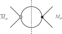
Figure 1: A diagram, whose imaginary part, denoted by the dotted line, represents the lifetime difference $y$. A white square represents a ${\cal H}_{\rm eff}^{\Delta L_{\mu}=2}$, while a black dot is the SM contribution of Equation (3).

Para-muonium. The relevant matrix elements of the spin-singlet state can be read off the Equation (3.2). Recalling the definitions in Equations (24) and (27), we obtain an expression for the lifetime difference $y_{P}$ for the para-muonium state,

$$y_{P}=\frac{G_{F}}{\sqrt{2}\Lambda^{2}}\frac{M_{M}^{2}}{\pi^{2}\Gamma}(m_{red}\alpha)^{3}\left(C_{6}^{\Delta L=2}-C_{7}^{\Delta L=2}\right).$$ (34)

One should note that if $C_{6}^{\Delta L=2}=C_{7}^{\Delta L=2}$ current conservation assures that no lifetime difference is generated at this order in $1/\Lambda$ for the para-muonium.

Ortho-muonium. Employing the matrix elements for the spin-triplet state computed in Equation (3.2), the lifetime difference for the vector muonia is

$$y_{V}=-\frac{G_{F}}{\sqrt{2}\Lambda^{2}}\frac{M_{M}^{2}}{\pi^{2}\Gamma}(m_{red}\alpha)^{3}\left(5C_{6}^{\Delta L=2}+C_{7}^{\Delta L=2}\right).$$ (35)

We emphasize that Equations (34) and (35) represent parametrically leading contributions to muonium lifetime difference, as they are only suppressed by two powers of $\Lambda$. Nevertheless, additional suppression by $G_{F}$ makes the observation of the lifetime difference in the muonium system extremely challenging.

3.4 Experimental Studies of Muonium Oscillations

Both $x$ and $y$ are the observable parameters, so experiments studying ${M_{\mu}}-{\overline{M}_{\mu}}$ oscillations could probe them by producing the ${M_{\mu}}$ state and looking for the decay products of the ${\overline{M}_{\mu}}$ state. Such experiments must overcome several considerable challenges.

First, muonium states must be produced inside the target and moved to the decay volume of the detector. The efficiency of such a process strongly depends on the target material. For example, the Muonium–Antimuonium Conversion Spectrometer (MACS) at PSI Willmann:1998gd used SiO₂ powder target with efficiency of 4–5%. A recently proposed Muonium-to-Antimuonium Conversion Experiment (MACE) MACE at the China Spallation Neutron Source (CSNS) will use an aerogel target with laser-drilled channels. The efficiency of producing muonia on such target could reach 40%.

Second, the strategy of looking for the “wrong-sign" final state, while working well in the studies of $B^{0}$ or $D^{0}$ oscillations, faces new challenges when applied to muonium oscillation searchers. The main reason is that the final state in the muonium decay ${M_{\mu}}\to e^{+}e^{-}\bar{\nu}_{\mu}\nu_{e}$ and that in the antimuonium decay ${\overline{M}_{\mu}}\to e^{+}e^{-}\bar{\nu}_{e}\nu_{\mu}$, differ only by the flavor combination of the neutrino states. Since the neutrinos are not detected, a method based on the kinematics of the decay must be employed: the decay products of the ${\overline{M}_{\mu}}$ involve fast electron with the momentum of about 53 MeV and slow positron with the momentum of about 13.5 eV. This follows from the fact that the main decay channel of the state is the decay of a muon.

Third, the experiments usually involve a setup where produced muonia propagate in the magnetic field $B_{0}$. This magnetic field suppresses oscillations by removing degeneracy between ${M_{\mu}}$ and ${\overline{M}_{\mu}}$ Li:2019xvv ; Hou:1995np . It also has a different effect on different spin configurations of the muonium state and the Lorentz structure of the operators that generate mixing Cuypers:1996ia ; Horikawa:1995ae . Fortunately, these effects can be taken into account. MACS experiment corrected the oscillation probability by introducing a factor $S_{B}(B_{0})$ Willmann:1998gd ,

$$P({M_{\mu}}\rightarrow{\overline{M}_{\mu}})\leq 8.3\times 10^{-11}/S_{B}(B_{0}).$$ (36)

The values of $S_{B}(B_{0})$, presented in Table II of Willmann:1998gd , are different for different values of magnetic field and chiral structure of the operators governing the $M_{\mu}-\overline{M}_{\mu}$ oscillations.

We can now use the derived expressions for $x$ and $y$ to place constraints on the BSM scale $\Lambda$ (or the Wilson coefficients $C_{i}$) from the experimental constraints on muonium–anti-muoium oscillation parameters. Since both spin-0 and spin-1 muonium states were produced in the experiment Willmann:1998gd , we should average the oscillation probability over the number of polarization degrees of freedom,

$$P({M_{\mu}}\rightarrow{\overline{M}_{\mu}})_{\rm exp}=\sum_{i=P,V}\frac{1}{2S_{i}+1}P({M_{\mu}}^{i}\rightarrow{\overline{M}_{\mu}}^{i}),$$ (37)

where $P({M_{\mu}}\rightarrow{\overline{M}_{\mu}})_{\rm exp}$ is the experimental oscillation probability from Equation (36). We shall use the values of $S_{B}(B_{0})$ for $B_{0}=2.8$ $\mu$T from the Table II of Willmann:1998gd , as it will provide us the best experimental constraints on the BSM scale $\Lambda$. We set the corresponding Wilson coefficient $C_{i}=1$. We report those constraints in Table 1.

Table 1: Constraints on the energy scales probed by different $\Delta L=2$ operators of Equations (1) and (7) in MACS experiment (from Conlin:2020veq ).

Operator	Interaction Type	$S_{B}(B_{0})$ (from Willmann:1998gd )	Scale $\Lambda$, TeV
$Q_{1}$	$(V-A)\times(V-A)$	0.75	$5.4$
$Q_{2}$	$(V+A)\times(V+A)$	0.75	$5.4$
$Q_{3}$	$(V-A)\times(V+A)$	0.95	$5.4$
$Q_{4}$	$(S+P)\times(S+P)$	0.75	$2.7$
$Q_{5}$	$(S-P)\times(S-P)$	0.75	$2.7$
$Q_{6}$	$(V-A)\times(V-A)$	0.75	$0.58\times 10^{-3}$
$Q_{7}$	$(V+A)\times(V-A)$	0.95	$0.38\times 10^{-3}$

As one can see from Equations (29), (31), (34) and (35), each observable depends on the combination of the operators. Assuming that only one operator at a time gives a dominant contribution, i.e., employing the single operator dominance hypothesis, it is possible to constrain the Wilson coefficients of each operator. While this ansatz is not necessarily realized in many particular UV completions of the LFV EFTs, as cancellations among contributions of different operators are possible, it is, however, a useful tool in constraining parameters of ${\cal L}_{\rm eff}$.

We must emphasize that the constraints presented in Table 1 use the data obtained more than twenty years ago! New results from new experiments are therefore highly desired. The MACE experiment MACE is expected to improve the sensitivity to $C_{i}^{\Delta L_{\mu}=2}/\Lambda^{2}$ by at least two orders of magnitude. A new experiment at J-PARC is also expected to improve the constraints on the muonium–antimuonium oscillation parameters Kawamura:2021lqk .

3.5 Constraints on Explicit Models of New Physics

It might be instructive to consider explicit models of new physics which could be probed by ${M_{\mu}}-{\overline{M}_{\mu}}$ oscillations. This approach lacks the universality of the EFT approach described above. However, what it lacks in the universality it compensates for in the applicability: new degrees of freedom introduced in explicit models can contribute to other processes, some of which might not even include FCNCs or muons. Even restricting our attention to the sector of those frameworks containing $\Delta L_{\mu}=1$ and/or $\Delta L_{\mu}=2$ interactions reveals such a multitude of models that reviewing each and every one of them here would be impractical. We will take another approach.

We will review two specific models, one with heavy NP particles (a doubly-charged Higgs model), and one with light NP states (a model with flavor-violating axion-like particle (ALPs)) as examples. Then we discuss classes of NP interactions that can be probed by muonium oscillations, and refer the readers to further examples.

One way to classify the models of NP that contribute to ${M_{\mu}}-{\overline{M}_{\mu}}$ mixing is by the masses of NP particles $m$. The models with heavy ($m\gg m_{M_{\mu}}$) new physics degrees of freedom can be matched to the effective Lagrangian of Equation (5). With that, experimental constraints on the parameters of this Lagrangian discussed in Section 3.4 and Table 1 lead to constraints on model parameters. The constraints on models with light ($m\leq m_{M_{\mu}}$) new physics degrees of freedom can be implemented within the framework of either concrete or simplified models.

Heavy new physics. Let us consider a model which contains a doubly-charged Higgs boson Swartz:1989qz ; Chang:1989uk ; Han:2021nod . Such states often appear in the context of left-right models Kiers:2005gh ; Kiers:2005vx , where an additional Higgs triplet is introduced to introduce neutrino masses

$$\Delta=\left({\begin{array}[]{cc}\Delta^{+}/\sqrt{2}&\Delta^{++}\\ \Delta^{0}&-\Delta^{+}/\sqrt{2}\\ \end{array}}\right)$$ (38)

A coupling of the doubly charged Higgs field $\Delta^{++}$ to the lepton fields can be written as

$${\cal L}_{R}=-\frac{1}{2}g_{\ell_{i}\ell_{j}}\overline{\ell}_{i}^{c}\Delta\ell_{j}+H.c.,$$ (39)

where $\ell^{c}=C\overline{\ell}^{T}$ is the charge-conjugated lepton state. Integrating out the $\Delta^{--}$ field, this Lagrangian leads to the following effective Hamiltonian Swartz:1989qz ; Kiers:2005vx

$${\cal H}_{\Delta}=-\frac{g_{ee}g_{\mu\mu}^{*}}{8M_{\Delta}^{2}}\left(\overline{\mu}_{L}\gamma_{\alpha}e_{L}\right)\left(\overline{\mu}_{L}\gamma^{\alpha}e_{L}\right)+H.c.,$$ (40)

below the scales associated with the doubly-charged Higgs field’s mass $M_{\Delta}$. Examining Equation (40) we see that this Hamiltonian matches onto our operator $Q_{2}$ (see Equation (1)) with the scale $\Lambda=M_{\Delta}$ and the corresponding Wilson coefficient $C_{2}^{\Delta L=2}=g_{ee}g_{\mu\mu}^{*}/8$.

The constraints on the masses and coupling constants depend on a particular model and other assumptions, such as whether the hierarchy of the neutrino masses is direct or inverse. It is however claimed that future experiments, such as MACE, could provide constraints on the doubly-charged Higgs state mass of $m_{\Delta}<3$ TeV Han:2021nod .

It is interesting to point out that such a doubly-charged scalar state would also contribute to the anomalous magnetic moment of the muon, both at one-loop Fukuyama:2009xk and at two-loops via the Barr-Zee type of mechanism Chen:2021jok . It was shown that $\Delta^{++}$ with the mass of a few hundred GeV could explain the discrepancy between the theoretical prediction and experimental measurement of $(g-2)$ of the muon Muong-2:2021ojo , particularly due to the enhancement from the two units of electric charge of the $\Delta^{++}$.

Light new physics. Let us consider a model with light axion-like particles that couple derivatively to the lepton current Endo:2020mev ; Calibbi:2020jvd . For the flavor off-diagonal interactions of the ALP $a$, the Lagrangian would contain a term

$${\cal L}_{\rm ALP}=\sum_{i\neq j}\frac{\partial_{\mu}a}{2f_{a}}\ \bar{\ell}_{i}\gamma^{\mu}\left(C_{\ell_{i}\ell_{j}}^{V}+C_{\ell_{i}\ell_{j}}^{A}\gamma_{5}\right)\ell_{j},$$ (41)

where $C_{\ell_{i}\ell_{j}}^{V,A}$ are Hermitian matrices of coupling constants, and $f_{a}$ is a decay constant related to the scale of the symmetry breaking associated with the ALP.

Since the mass of the ALP, $m_{a}$, is a free parameter, it is possible that, while $a$ is light, to have $m_{a}>m_{M_{\mu}}$. In this case the ALP can be integrated out and the constraints from the Table 1 imply that Calibbi:2020jvd

$$\frac{1}{3.8\ \mbox{TeV}}>\frac{1}{2f_{a}}\left|\left(C_{\mu e}^{A}\right)^{2}-\left(C_{\mu e}^{V}\right)^{2}\right|^{1/2}\left(\frac{m_{\mu}}{m_{e}}\right).$$ (42)

In the opposite case $m_{a}<m_{M_{\mu}}$ the constraint can be obtained by taking a limit $m_{\mu}/m_{a}\to 1$ Calibbi:2020jvd . Note that in both cases one can only constrain the combination $C_{\mu e}^{V,A}/f_{a}$. These results have direct implications for ALP contributions to muon $(g-2)$ Endo:2020mev (c.f., Bauer:2019gfk ), the cross-section of $e^{+}e^{-}\to ee\mu\mu$ Calibbi:2020jvd , and other quantities.

A useful classification of lepton-flavor-violating interactions probed by the muonium oscillations was given in Fukuyama:2021iyw . Such interactions can be classified by the way they break the lepton flavor.

1. $\Delta L_{e}=\Delta L_{\mu}=0$. In such models, the interactions do not violate lepton flavor quantum numbers. The muonium oscillations are induced at one-loop order by the mass terms of the fields that transform as singlets under the SM gauge group and have $L_{e,\mu}=\pm 2$. Examples of such models include constructions with Majorana neutrinos ClarkLove:2004 ; Fukuyama:2021iyw .

2. $\Delta L_{e}=\pm 2,\Delta L_{\mu}=0$ and $\Delta L_{e}=0,\Delta L_{\mu}=\pm 2$. In such models, the lepton flavor quantum numbers are separately broken. The mediators of such interactions, sometimes called dilepton bosons, have electric charge $2e$ and lepton number equal to two. The mediators could be scalar or vector bosons. Examples of such models include the doubly-charged Higgs model considered above Cuypers:1996ia ; Horikawa:1995ae ; Swartz:1989qz ; Chang:1989uk ; Han:2021nod ; Fukuyama:2009xk ; Chen:2021jok and many other constructions Fukuyama:2021iyw . Muonium oscillations can be generated at tree level in such models.

3. $\Delta L_{e}=-\Delta L_{\mu}=\pm 1$. In such models, interaction terms violate both lepton flavor numbers. The mediators of such interactions are electrically neutral and could be both scalar and vector bosons. Examples of such models include models with flavor-violating Higgs boson Harnik:2012pb , and many others Fukuyama:2021iyw . Muonium oscillations can also be generated at the tree level in such models. These models can also be probed in muon conversion experiments unless the mediator is introduced such that it only interacts with the leptons.

4. $\Delta L_{e}=\pm 1,\Delta L_{\mu}=0$ and $\Delta L_{e}=0,\Delta L_{\mu}=\pm 1$. In such models, effective operators mediating muonium oscillations are generated at one-loop order. These models can also be probed in other muon transitions, such as $\mu\to 3e$.

As was pointed out in Fukuyama:2021iyw if a $Z_{n}$ discrete symmetry is imposed to suppress the $\Delta L_{e}-\Delta L_{\mu}=\pm 1$ interactions, while allowing for $\Delta L_{e}-\Delta L_{\mu}=\pm 2$ terms, the oscillation rates are not well-probed by other experiments and can be as large as allowed by the current experimental bound. Clearly, ${M_{\mu}}-{\overline{M}_{\mu}}$ oscillations probe a wide variety of NP models and serve as effective tools that are complementary to other searches.

4 Muonium Decays

Processes that change lepton flavor by two units can, in principle, also be studied in the decays of muons and muonia. The transitions into neutrino states, governed by the operators in Equation (7), fit the bill. The decay rate for such transition is

$$\Gamma\left({M_{\mu}^{V}}\to\bar{\nu}_{e}\nu_{\mu}\right)=\frac{f_{M}^{2}M_{M}^{3}}{9\pi\Lambda^{4}}\left|C_{6}^{\Delta L_{\mu}=2}+C_{7}^{\Delta L_{\mu}=2}\right|^{2}.$$ (43)

Note that in the limit of massless neutrinos only the spin-one ortho-muonium state would have non-zero width. While the invisible decays of the spin-zero para-muonium would not be strictly forbidden in this limit, as they would be dominated by the four-neutrino final state Bhattacharya:2018msv , the decay rate of the para-muonium would be very small.

The decay rate of Equation (43) will add incoherently to the SM decay rate

$$\Gamma\left({M_{\mu}^{V}}\to\bar{\nu}_{\mu}\nu_{e}\right)=\frac{G_{F}^{2}f_{M}^{2}M_{M}^{3}}{12\pi}.$$ (44)

Even in the SM, this is a very rare process. Numerically, the branching fraction can be computed to be

$${\cal B}\left({M_{\mu}}\to\bar{\nu}_{\mu}\nu_{e}\right)=6.6\times 10^{-12}.$$ (45)

Both decays contribute to the “invisible" width of the muonium,

$$\Gamma\left({M_{\mu}^{V}}\to\mbox{invisible}\right)=\Gamma\left({M_{\mu}^{V}}\to\bar{\nu}_{\mu}\nu_{e}\right)+\Gamma\left({M_{\mu}^{V}}\to\bar{\nu}_{e}\nu_{\mu}\right)+...,$$ (46)

where ellipses denote decays into multineutrino states, which are further suppressed by the phase space factors.

Experimental studies of the invisible width of muonia are very challenging. One possibility to constrain the invisible width indirectly Gninenko:2012nt involves comparing the measurements of the positively-charged muon lifetime inside the material, where it forms the muonia and that of the free muon. Since the lifetime difference between the muonium in the target and free muon in vacuum was estimated to be negligible Czarnecki:1999yj , the possible difference can be ascribed to the invisible width of the muonium. Using the lifetime measurements performed by the MuLan Collaboration MuLan:2007qkz , the limit

$${\cal B}\left({M_{\mu}}\to\mbox{invisible}\right)<5.7\times 10^{-6}$$ (47)

can be established at 90% C.L. Gninenko:2012nt with an assumption that the fraction of triplet muonium state in the MuLan’s quartz target is 3/4. This bound does not yet provide a meaningful probe of either an SM process of Equation (44) or the $\Delta L_{\mu}=2$ process of Equation (43).

A more sensitive probe of the $\Delta L_{\mu}=2$ process does not require a muonium bound state and can be obtained by comparing the lifetime of the muon in a vacuum to theoretical prediction in the framework of the standard model. The results will be reported elsewhere.

5 Conclusions

Muonium is the simplest QED bound state. Yet, it holds the potential to probe new physics in ways that are unique and complementary to other NP searches with muons. In this review, we discussed how lepton-flavor violating $\Delta L_{\mu}=2$ transitions could be probed in the muonium system, both in muonium decays and in muonium–antimuonium oscillations. We discussed the phenomenology of such oscillations, arguing that the presence of $\Delta L_{\mu}=2$ interactions would lead to both mass and lifetime splittings in the muonium–antimuonium system. We showed how to compute those oscillation parameters in an effective field theory approach, showing that both parameters scale as $1/\Lambda^{2}$ with respect to the new physics scale $\Lambda$.

We discussed the current status and future perspectives of experiments that can constrain muonium–antimuonium oscillation parameters, and how such measurements can be used to place bounds on the parameters of the effective Lagrangians governing the $\Delta L_{\mu}=2$ transitions. These bounds can be further translated into the constraints on the masses and couplings of new particles in specific models of new physics, and, in case of the observation of the oscillation phenomena would help us to identify the proper extension of the standard model.

This research was supported in part by the U.S. Department of Energy grant No. DE-SC0007983 and by the Excellence Cluster ORIGINS, which is funded by the Deutsche Forschungsgemeinschaft (DFG, German Research Foundation) under Germany’s Excellence Strategy —EXC-2094—390783311. AAP was also supported by the Visiting Scholars Award Program of the Universities Research Association. Fermilab is managed and operated by Fermi Research Alliance, LLC under Contract No. DE-AC02-07CH11359 with the U.S. Department of Energy.

Not applicable.

Not applicable.

Not applicable.

- (1) Petrov, A.A. Indirect Searches for New Physics; CRC Press: Boca Raton, FL, USA, 2021. http://doi.org/10.1201/9781351176019.
- (2) Grzadkowski, B.; Iskrzynski, M.; Misiak, M.; Rosiek, J. Dimension-Six Terms in the Standard Model Lagrangian. JHEP 2010, 10, 085.
- (3) Petrov, A.A.; Blechman, A.E. Effective Field Theories; World Scientific: Singapore, 2016. http://doi.org/10.1142/8619.
- (4) Celis, A.; Cirigliano, V.; Passemar, E. Model-discriminating power of lepton flavor violating decays. Phys. Rev. D 2014, 89, 095014.
- (5) Hazard, D.E.; Petrov, A.A. Radiative lepton flavor violating B, D, and K decays. Phys. Rev. D 2018, 98, 015027.
- (6) Hazard, D.E.; Petrov, A.A. Lepton flavor violating quarkonium decays. Phys. Rev. D 2016, 94, 074023.
- (7) Conlin, R.; Petrov, A.A. Muonium–antimuonium oscillations in effective field theory. Phys. Rev. D 2020, 102, 095001.
- (8) Grossman, Y.; Isidori, G.; Murayama, H. Lepton flavor mixing and decays. Phys. Lett. B 2004, 588, 74–80.
- (9) Tanabashi, M.; Hagiwara, K.; Hikasa, K.; Nakamura, K.; Sumino, Y.; Takahashi, F.; Tanaka, J.; Agashe, K.; Aielli, G.; Amsler, C.; et al. Review of Particle Physics. Phys. Rev. D 2018, 98, 030001.
- (10) Czarnecki, A.; Lepage, G.; ; Marciano, W.J. Muonium decay. Phys. Rev. D 2000, 61, 073001.
- (11) Pontecorvo, B. Mesonium and anti-mesonium. Sov. Phys. JETP 1957, 6, 429.
- (12) Feinberg, G.; Weinberg, S. Conversion of Muonium into Antimuonium. Phys. Rev. 1961, 123, 1439–1443.
- (13) Clark, T.E.; Love, S.T. Muonium–Antimuonium oscillations and massive Majorana neutrinos. Mod. Phys. Lett. 2004, A19, 297.
- (14) Cvetic, G., Dib, C.O., Kim, C., Kim, J., Muonium–antimuonium conversion in models with heavy neutrinos. Phys. Rev. D 2005, 71, 113013.
- (15) Li, T., Schmidt, M.A., Sensitivity of future lepton colliders and low-energy experiments to charged lepton flavor violation from bileptons. Phys. Rev. D 2019, 100, 115007.
- (16) Endo, M.; Iguro, S.; Kitahara, T. Probing flavor-violating ALP at Belle II. JHEP 2020, 6, 040.
- (17) Bernstein, R.H.; Cooper, P.S. Charged Lepton Flavor Violation: An Experimenter’s Guide. Phys. Rept. 2013, 532, 27–64.
- (18) Willmann, L.; Schmidt, P.V.; Wirtz, H.P.; Abela, R.; Baranov, V.; Bagaturia, J.; Bertl, W.; Engfer, R.; Grossmann, A.; Hughes, V.W.; et al. New bounds from searching for muonium to anti-muonium conversion. Phys. Rev. Lett. 1999, 82, 49–52.
- (19) Donoghue, J.F.; Golowich, E.; Holstein, B.R. Dynamics of the Standard Model; Cambridge Univ. Press: Cambridge, UK, 1994
- (20) Nierste, U. Three Lectures on Meson Mixing and CKM phenomenology. arXiv 2009, arXiv:0904.1869.
- (21) Golowich, E.; Pakvasa, S.; Petrov, A.A. New Physics contributions to the lifetime difference in mixing. Phys. Rev. Lett. 2007, 98, 181801.
- (22) Tang, J., Chen, Y., Mao, Y.-Z., Bao, Y., Chen, Y.-K., Fan, R.-R., Hou, Z.-L., Jing, H.-T., et al. Letter of Interest Contribution to Snowmass 2021. 2020. Available online: https://www.snowmass21.org/docs/files/summaries/RF/SNOWMASS21-RF5_RF0_Jian_Tang-126.pdf (accessed on 05 March 2022).
- (23) Hou, H.S.; Wong, G.G. Magnetic field dependence of muonium–anti-muonium conversion. Phys. Lett. B 1995, 357, 145–150.
- (24) Cuypers, F.; Davidson, S. Bileptons: Present limits and future prospects. Eur. Phys. J. C 1998, 2, 503–528.
- (25) Horikawa, K.; Sasaki, K. Muonium–anti-muonium conversion in models with dilepton gauge bosons. Phys. Rev. D 1996, 53, 560–563.
- (26) Kawamura, N.; Kitamura, R.; Yasuda, H.; Otani, M.; Nakazawa, Y.; Iinuma, H.; Mibe, T. A new approach for Conversion Search. JPS Conf. Proc. 2021, 33, 011120. http://doi.org/10.7566/JPSCP.33.011120.
- (27) Swartz, M.L. Limits on Doubly Charged Higgs Bosons and Lepton Flavor Violation. Phys. Rev. D 1989, 40, 1521.
- (28) Chang, D.; Keung, W.Y. Constraints on Muonium–anti-Muonium Conversion. Phys. Rev. Lett. 1989, 62, 2583.
- (29) Han, C.; Huang, D.; Tang, J.; Zhang, Y. Probing the doubly charged Higgs boson with a muonium to antimuonium conversion experiment. Phys. Rev. D 2021, 103, 055023.
- (30) Kiers, K.; Assis, M.; Petrov, A.A. Higgs sector of the left-right model with explicit CP violation. Phys. Rev. D 2005, 71, 115015.
- (31) Kiers, K.; Assis, M.; Simons, D.; Petrov, A.A.; Soni, A. Neutrinos in a left-right model with a horizontal symmetry. Phys. Rev. D 2006, 73, 033009.
- (32) Fukuyama, T.; Sugiyama, H.; Tsumura, K. Constraints from muon g-2 and LFV processes in the Higgs Triplet Model. JHEP 2010, 3, 044.
- (33) Chen, C.H.; Chiang, C.W.; ; Nomura, T. Muon g-2 in a two-Higgs-doublet model with a type-II seesaw mechanism. Phys. Rev. D 2021, 104, 055011.
- (34) Abi, B.; Albahri, T.; Al-Kilani, S.; Allspach, D.; Alonzi, L.P.; Anastasi, A.; Anisenkov, A.; Azfar, F.; Badgley, K.; Baeßler, S.; et al. Measurement of the Positive Muon Anomalous Magnetic Moment to 0.46 ppm. Phys. Rev. Lett. 2021, 126, 141801.
- (35) Calibbi, L.; Redigolo, D.; Ziegler, R.; Zupan, J. Looking forward to lepton-flavor-violating ALPs. JHEP 2021, 9, 173.
- (36) Bauer, S.; Neubert, M.; Renner, S.; Schnubel, M.; Thamm, A. Axionlike Particles, Lepton-Flavor Violation, and a New Explanation of and . Phys. Rev. Lett. 2020, 124, 211803.
- (37) Fukuyama, T.; Mimura, Y.; Uesaka, Y. Models of the Muonium to Antimuonium Transition. Phys. Rev. D 2022, 105, 015026.
- (38) Harnik, R.; Kopp, J.; Zupan, J. Flavor Violating Higgs Decays. JHEP 2013, 3, 026.
- (39) Bhattacharya, B.; Grant, C.M.; Petrov, A.A. Invisible widths of heavy mesons. Phys. Rev. D 2019, 99, 093010.
- (40) Gninenko, S.N.; Krasnikov, N.V.; Matveev, V.A. Invisible Decay of Muonium: Tests of the Standard Model and Searches for New Physics. Phys. Rev. D 2013, 87, 015016.
- (41) Chitwood, D.B.; Banks, T.I.; Barnes, M.J.; Battu, S.; Carey, R.M.; Cheekatmalla, S.; Clayton, S.M.; Crnkovic, J.; Crowe, K.M.; Debevec, P.T.; et al. Improved measurement of the positive muon lifetime and determination of the Fermi constant. Phys. Rev. Lett. 2007, 99, 032001.