Easy Ensemble: Simple Deep Ensemble Learning for Sensor-Based Human Activity Recognition

Abstract

Sensor-based human activity recognition (HAR) is a paramount technology in the Internet of Things services. HAR using representation learning, which automatically learns a feature representation from raw data, is the mainstream method because it is difficult to interpret relevant information from raw sensor data to design meaningful features. Ensemble learning is a robust approach to improve generalization performance; however, deep ensemble learning requires various procedures, such as data partitioning and training multiple models, which are time-consuming and computationally expensive. In this study, we propose Easy Ensemble (EE) for HAR, which enables the easy implementation of deep ensemble learning in a single model. In addition, we propose input masking as a method for diversifying the input for EE. Experiments on a benchmark dataset for HAR demonstrated the effectiveness of EE and input masking and their characteristics compared with conventional ensemble learning methods.

Keywords Human Activity Recognition  $\cdot$ Context-awareness  $\cdot$ Ensemble Learning  $\cdot$ Deep Learning

1 Introduction

With the widespread of Internet of Things (IoT) devices, sensor values can be easily collected and applied to human activity recognition (HAR). In HAR, IoT sensors are appropriate for recording the behavior of individuals who move around compared to a fixed camera. In other words, HAR is a vital application of IoT technology. It is difficult for humans to interpret the context of raw sensor values and human behavior differs among individuals; therefore, automatic feature extraction by deep representation learning is used to build HAR models. To develop an accurate HAR model, researchers have investigated various model architectures [1, 2, 3] using deep learning in the image recognition field.

Because IoT devices can be easily equipped with many places, multiple sensor modalities are generally used as inputs for the the HAR models. For example, the well-known public benchmark HAR dataset PAMAP2 [4] uses a heart rate sensor and three wireless inertial measurement units (IMUs). The IMUs are equipped at the wrist, chest, and ankle to measure temperature, three-axis acceleration (two scales), three-axis gyro, and three-axis geomagnetism. Althoug the shape of an input tensor in image recognition is commonly fixed to three RGB channels, many HAR studies use multidimensional sensor data as input. HAR sometimes applies ensemble learning [5, 6] to assign independent feature extractors for each sensor modality. Separate feature extractors for each sensor modality are generally superior to a single feature extractor that uses concatenated input data. As an advanced technique, a method that performs masking based on a multinomial distribution when merging each feature representation [7] and another that ensembles feature extractors by grouping them based on sensor features [8] have also been proposed. Thus, the use of ensemble learning is more crucial in HAR than image recognition.

Ensemble learning is a simple strategy that can significantly enhance generalization performance, not only for HAR but also for various machine learning tasks. Ensemble learning is a general term for machine learning methods that use multiple models together, and it generally improves generalization performance compared with a single model. Ensemble learning is also a robust technique in deep learning. However, the computation and implementation costs are higher than those of a single model because multiple models must be trained individually, and then the models must be combined during inference to perform different behaviors than during training. Although a technique to reduce the computational cost by sharing model parameters [9] has been proposed, its implementation is complicated.

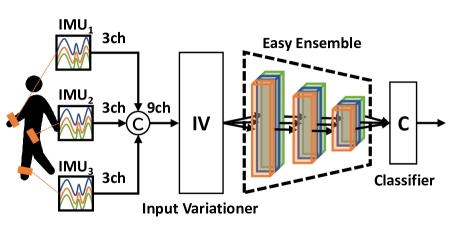
Figure 1: EE and input variationer make it possible to easily use a deep ensemble learning model for HAR.

In this study, we propose a simple and easy-to-implement deep learning ensemble method –Easy Ensemble (EE)– to improve the complexity of training and inference (Fig. 1). EE is a method that treats the input channels as $N$ groups internally, each of which performs feature extraction independently. Perticularly, we aim to realize an easy-to-implement deep ensemble learning method and not to reduce computational cost. We employ several benchmark datasets to demonstrate the effectiveness of EE and clarify factors contributing to the improvement of EE accuracy and characteristics of EE as each parameter or input is varied. Further, we propose a new input diversification method for EE –input variationer– and demonstrate its effectiveness in improving the generalization performance by adding a variety to the input.

2 Related works

2.1 Ensemble learning in HAR

Many studies have employed ensemble learning methods using hand-crafted features as an application of ensemble learning in HAR [10, 11, 12, 13]. Ensemble methods have also been proposed for deep learning. Zhu et al.[14] proposed a method that builds multiple classifiers using hand-crafted features, then uses convolutional neural networks (CNNs) to learn feature representations from raw data, and determines the final output using weighted voting. Semwal et al. [15] proposed a method to combine the outputs obtained using four models in parallel, each of which is a CNN connected with long short-term memory (LSTM), and then obtain the final output through a fully-connected layer. In most methods that do not use deep learning, the final output is determined by majority vote, weighted sum, or rule-based method from the outputs of multiple models. When deep learning is used, the acquired feature representations can be combined and connected to a new fully-connected layer, as described by Semwal et al. [15]

2.2 Ensemble method in deep learning

Although ensemble learning improves the generalization performance of models, the training time and memory cost required for one model are high in deep learning. Several methods have been proposed to mitigate this issue in image recognition.

Lee et al. [16] experimentally demonstrated an effective deep ensemble method. From the results, they proposed a method of ensembling while suppressing the number of parameters using TreeNets, a tree-structured model in which the lower layers share parameters, but the upper layers do not. It is preferable to merge values before the softmax function is applied instead of values that imitate the probability distribution after the softmax function is applied.

Wen et al. [17] proposed a Batch Ensemble, which suppresses the number of parameters by representing multiple models to be ensembled as a Hadamard product of shared parameters ${\bm{W}}$ and a trainable rank-1 matrix ${\bm{F}_{i}}$. Similarly, Wasay et al. [9] proposed MotherNets, which shares the parameters of common substructures in a model. Models with multiple architectures were classified by clustering, and a common substructure (MotherNet) was manually constructed within each cluster. MotherNet is first pretrained and then restored to its original structure by adding a small noise to the trained parameters. Subsequently, each model is additionally trained, which enables the fast training of ensemble models.

Havasi et al. [18] stated that although some ensemble methods based on parameter sharing reduce memory cost, their inference speed is decreased due to multiple forward paths. They proposed multi-input multi-output, which improves ensemble performance by increasing the number of inputs and outputs while sharing the model itself.

Because image recognition uses massive high-resolution data, the training time and memory cost are significant issues. Moreover, in the HAR field, the input data are waveform data and training datasets are not as large as those of image recognition. Therefore, it is necessary to find a method to facilitate the implementation of ensemble learning to improve accuracy.

2.3 Analysis on deep-learning ensembling

Although ensemble learning contributes to improving estimation accuracy because of its diversification, these exist some unexplained aspects. Wasay et al. [19] experimentally analyzed the performance of CNNs in image recognition, comparing an ensemble of multiple models with few parameters to a single model with the same number of parameters. By comparing several image recognition benchmarks, they found that ensemble learning needs to have a certain number of parameters to be effective and that the more complex the dataset is, the more effective the ensemble learning will be.

Allen-Zhu et al. [20] reported that increasing estimation accuracy using a deep ensemble learning and knowledge distillations [21] is a mystery . In an experiment using CIFAR-100, the average test accuracy of 10 individual models was 81.51%, but the ensemble of weighted averaging of the output of each model improved the test accuracy to 84.69%. However, training all models together by optimizing the sum of each model did not produce such an improvement in accuracy, resulting in a test accuracy of 81.83%. Thus, in ensemble models with the same initial values, training the models aggregating outputs does not provide the ensemble benefit. In other words, individual training contributes to the acquisition of diversity rather than the effect of larger models.

2.4 Ensemble learning with group convolution

The novelty of our proposed method is that it uses grouping modules (group convolution, etc.) to build an ensemble characteristic in a single model. Group convolution has been used in the early years of deep learning. AlexNet has multiple CNN paths for parallel processing of multiple convolutions on multiple graphics processing units. In addition, ResNeXt [22] introduces the concept of “Cardinality,” which splits convolution in the residual block of ResNet [23] into multiple convolutions to improve accuracy. “Cardinality” can be implemented using multiple convolution layers, which is also equivalent to using group convolution.

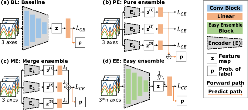
Figure 2: Model architecture of our proposed EE method and common ensemble of deep learning.

The method most similar to EE is the Group Ensemble (GE) proposed by Chen et al. [24], which uses group convolution to make an ensemble learning in a single model for image recognition. Particularly, Chen et al. [24] proposed sharing low layers and using random weights to combine multiple outputs. However, their algorithm was not described in detail. Moreover, there is no discussion on the equivalence before and after ensembling, normalization method, number of parameters, ablation study, and so on. There is also no discussion on input diversification because the lower layers are shared.

2.5 Position of this study

In this study, we aim to realize a learning method that reduces the complexity of training and inference for ensemble learning while maintaining the advantages of ensemble learning. The novelty of this study is that it focuses on realizing a method that is easy to implement and use rather than on reducing training time and memory cost.

The contributions of this study are as follows.

• We propose the EE algorithm, which enables various model architectures to be an ensemble model in a single model, and show that EE is equivalent to the ensemble method with majority voting.

• We proposed input variationer, which provides a variety of inputs and an input procedure for environments with multiple types of sensor modalities when multiple IoT devices are used together.

• Using a benchmark dataset for HAR, we clarified the characteristics of EE under various conditions.

3 EE

3.1 Ensemble models in deep learning

Fig. 2 shows model outlines of EE and the general ensemble of deep learning methods. As shown in Fig. 2 (a), raw sensor data are input into the feature extractor –Encoder (E)– in the general CNN model, and an extracted feature vector $\bm{z}$ is transformed into the probability distribution of activity label $\bm{p}$ through a fully-connected layer and the softmax function (hereinafter baseline (BL)). The parameters of the entire model were trained based on the categorical cross-entropy loss using $\bm{p}$ with a correct label.

Although various ensemble methods have been proposed for deep learning [Fig. 2 (b)], bagging-like ensemble is commonly used (hereinafter, pure ensemble (PE)). Assuming that the number of ensembles is $N$ (for example $N=3$ in Fig. 2), PE inputs raw sensor values to the $N$ models, each of which is trained independently. In the original bagging algorithm, multiple subsets are constructed from the original training dataset, and each model is trained using each subset; however, in this section, the same input is used to simplify the explanation of EE. A discussion of the input style is described in Section 5.1.

While PE improves the generalization performance, it requires that $N$ models are trained by calculating the loss function $N$ times for each path during training because there are multiple outputs. Further, the inference path differs from the training path, which increases implementation cost. Therefore, when applying an ensemble in deep learning [Fig. 2 (c)], a method that unifies the outputs of each path and uses weighted summation by weight coefficients $\{\lambda_{1},\lambda_{2},\lambda_{3}\}$ is generally adopted (hereinafter, merge ensemble (ME)). ME improves the multioutput nature of PE and is expected to improve generalization performance by ensemble learning with a single-input single-output model. However, it lacks ease of operation because it requires the management of multiple models.

In this study, we propose EE, which improves the need to manage multiple models in ME. The advantages of EE are that it is as tractable and easy to implement as the BL model. $N$-times repeated inputs in the channel direction are independently processed in the EE block (EE-Block) as $N$ groups of channels. EE is a method to realize multiple encoders of ME in a single model. ResNeXt is similar to the transformed each module of ResNet to EE style (with different details such as normalization methods). In other words, EE is a generalization of the concept of “Cardinality” in ResNeXt.

As shown in Fig. 2 (d), the model architecture of EE is almost the same as that of BL, with the only differences being that the $N$ inputs to be ensembled are concatenated in the channel direction and the internal module that constitutes E is changed from the general convolutional block to EE-Block. Therefore, EE is easy to handle as a BL model in that it has a single input, output, and model.

3.2 EE-Block

The currently proposed modules of various CNNs can be easily converted into EE by simply changing some layers and hyperparameters. First, we list the typical layers used in existing CNNs. For example, in a visual geometry group (VGG) [25], the encoder comprises a convolutional layer, normalization layer, activation function, and pooling layer. In addition, Xception [26] uses depth-wise separable convolution, which divides the convolution layer into a depth and a point-wise convolution layer to reduce the number of parameters. ResNet [23] uses a shortcut connection that enables skipping some layers to remove the vanishing gradient issue. Most CNNs are realized by combining these layers.

By modifying each of the abovementioned layer as follows, all CNN modules can be EE style.

• Set the hyperparameter of groups as $N$ of the convolution layer to change to group convolution (same for the point-wise convolution layer).

• Change normalization layer to group normalization [27] by setting the group parameter to $N$.

• Because the fully-connected layer is equivalent to a one-dimensional convolution layer with a kernel size of 1, change the fully-connected layer to reshape and the group convolution layer.

• Multiply output $\bm{z}$ of E by $\frac{1}{N}$.

Notably, the activation function, pooling layer, depth-wise convolution layer, and shortcut connection are processed independently in the channel direction; therefore, they do not need to be changed. Using these simple procedures, all CNN architectures can be in the EE style.

EE is easy to implement using mainstream deep-learning libraries, such as Pytorch and TensorFlow. Because they have a group hyperparameter in the convolution layer, EE can only be implemented by setting the group parameter to $N$ when building the BL model. Further, these libraries have a group normalization layer; thus, only replacing normalization layers with group normalization layers is necessary. Implementing EE requires approximately the same amount of effort as implementing BL. Source code is made available at https://github.com/t-hasegawa-FU/Easy-Ensemble

3.3 Proof of equality between ME and EE

We describe the equality between ME and EE [Fig. 2 (c) and (d)] via the proof of equality in each layer type.

3.3.1 Convolution layer

$\bm{X}=[\bm{x}_{1},\bm{x}_{2},\cdots,\bm{x}_{n}]$ denotes input tensor. Here each $\bm{x}_{i}$ is a waveform sensor value in channel $i$, and $n$ is the total number of channels. Three-axis acceleration sensor values (x, y, and z) are commonly used as inputs in HAR. $\bm{Z}=[\bm{z}_{1},\bm{z}_{2},\cdots,\bm{z}_{m}]$, which is the output of a single convolution layer in ME, can be calculated as follows:

$$\bm{z}_{i}=\sum_{j=1}^{n}\bm{x}_{j}*\bm{w}_{i,j}+b_{i}$$ (1)

where $\bm{w}$ and $b$ denote the filter and bias of the convolution layer, respectively, and $*$ is the cross-correlation operator.

By contrast, the input tensor in EE is defined as $\bm{X^{\prime}}=[\bm{x}_{1},\bm{x}_{2},\cdots,\bm{x}_{n\times N}]$ because the input is repeated $N$ times in the channel direction in advance, where $N$ denotes the number of ensembles. $\bm{Z^{\prime}}=[\bm{z}_{1},\bm{z}_{2},\cdots,\bm{z}_{m\times N}]$, which is the output of a single group convolution layer in EE, can be calculated as follows:

$$\bm{z}_{i}=\left\{\begin{array}[]{ll}\sum_{j=1}^{n}\bm{x}_{j}*\bm{w}_{i,j}+b_{i}&(i\leq m)\\ \sum_{j=1}^{n}\bm{x}_{n+j}*\bm{w}_{i,j}+b_{i}&(m<i\leq 2m)\\ \vdots&\vdots\end{array}\right.$$ (2)

Group convolution, as defined, divides the input channel into $N$ equal groups and performs an operation to convolute independent parameters into each group. Therefore, $\bm{Z^{\prime}}$ is equivalent to the output of combining $\bm{Z}^{(1)},\bm{Z}^{(2)},\bm{Z}^{(3)}$ through $N$ individual convolution layers.

3.3.2 Normalization layer

To be EE, all normalization layers need to be group normalization layers. Although ME and EE are not completely equivalent when the normalizations are batch normalizations, assuming that all normalizations in ME are layer normalizations, ME and EE completely equivalent.

Layer normalization in ME normalizes input tensor $\bm{X}$ as follows:

$$\bm{Z}=\frac{\bm{X}-\bar{\bm{X}}}{\sqrt{(Var(\bm{X})+\epsilon)}}$$ (3)

where $Var(\bm{X})$ denotes the variance of $\bm{X}$, $\epsilon$ denotes a small constant (1e-05 in this study). Some implementations may use trainable scaling parameters, but we do not use them in EE.

In group normalization, combined input tensor $\bm{X^{\prime}}=[\bm{X}^{(1)},\bm{X}^{(2)},\cdots,\bm{X}^{(N)}]$ (the shape of each $\bm{X}^{(i)}$ is as same as $\bm{X}$) is normalized to output $\bm{Z^{\prime}}=[\bm{Z}^{(1)},\bm{Z}^{(2)},\cdots,\bm{Z}^{(N)}]$ as follows:

$$\bm{Z}^{(i)}=\frac{\bm{X}^{(i)}-\bar{\bm{X}}^{(i)}}{\sqrt{(Var(\bm{X}^{(i)})+\epsilon)}}$$ (4)

Group normalization, as defined, divides the input channel into $N$ equal groups and applies layer normalization to each group. Therefore, $\bm{Z^{\prime}}$ is equivalent to the output of each layer normalization combined $N$ times.

3.3.3 Fully-connected layer

$\bm{v}=[v_{0},v_{1},\cdots,v_{n}]\in\mathbb{R}^{n}$ denotes the input to a fully-connected layer. According to Equation (1), transform $\bm{v}$ into $\bm{V}\in\mathbb{R}^{n\times 1}$ and input it into convolution layer with kernel size of 1, and each element $\bm{z}_{i}$ of output $\bm{Z}\in\mathbb{R}^{m\times 1}$ is calculated as follows:

$$\bm{z}_{i}=\sum_{j=1}^{n}\bm{v}_{j}*\bm{w}_{i,j}+b_{i}$$ (5)

where each $\bm{z}_{i},\bm{v}_{j},\bm{w}_{i,j}$ is substantially a scalar. Thus, the element is as follows:

$$z_{i}=\sum_{j=1}^{n}v_{j}\cdot w_{i,j}+b_{i}$$ (6)

As Equation (6) is equivalent to the definition of a fully-connected layer, the fully-connected layer can be represented by a single convolution layer by reshaping input $\bm{v}$ to $\bm{V}\in\mathbb{R}^{n\times 1}$ and output $\bm{Z}$ to $\bm{z}\in\mathbb{R}^{m}$. Thus, as shown in Subsection 3.3.1, the fully-connected layer can be EE style by setting groups in the transformed convolution layer.

3.3.4 Pooling and output layers

The pooling layer applied between each layer is processed channel-independently and does not affect EE. The encoder output $\bm{z}$ in Fig. 2 (d) is a feature vector of length $m\times N$ obtained by applying global average pooling (GAP) to the final output $\bm{Z}$ of EE-Blocks. The GAP also calculates the average for each channel and does not affect EE.

Finally, using the feature vector $\bm{z}$, weight hyperparameter $\lambda=\frac{1}{N}$, and a single fully-connected layer, EE outputs $\bm{p}$ (applying the softmax function to $\bm{p}$ implies a class probability distribution) as follows:

$$\bm{p} = \frac{1}{N}\sum_{i=1}^{m\times N}z_{i}w_{i}+b$$ (7)

$$= \frac{1}{N}(\sum_{i=1}^{m}z_{i}w_{i}+\cdots+\sum_{i=(N-1)m+1}^{m\times N}z_{i}w_{i})+b$$

Here, each member expanded by Equation (7) is equivalent to the output of each path in Fig. 2 (c). Denoting $\lambda=\frac{1}{N}$, Figs. 2 (c) and (d) are equivalent. By vectorizing $\lambda$, it is also possible to set individual weight coefficients for each group, as in Chen et al.’s GE [24]. However, the verification results did not show any improvement in accuracy; therefore, the same value of $\lambda=\frac{1}{N}$ was used in this study.

EE is a single-model architecture similar to BL but requires multiplying $\lambda$ by the encoder’s output $\bm{z}$. In general, a classification model is optimized based on categorical cross-entropy loss using output $\bm{p}$ normalized by the softmax function, as follows:

$$Softmax(p_{i},\bm{p})=\frac{\exp(\frac{p_{i}}{T})}{\sum_{p_{j}\in\bm{p}}\exp(\frac{p_{j}}{T})}$$ (8)

where $\bm{p}$ denotes the output vector, $p_{i}$ denotes each element of $\bm{p}$, and is the normalization target. Because EE is equivalent to ME as mentioned above, calculating the predicted label $p_{i}$ for each path in ME without multiplying by $\lambda$ would result in $N$ times the scale of $p_{i}$ compared with BL. In Equation (8), $T$ is a temperature parameter that works as the general softmax function at $T=1$, emphasizing higher and lower values when $T<1$ and $T>1$ respectively. The predicted label $p_{i}$ multiplied by $N$ is the same as the temperature parameter $T=\frac{1}{N}$ in the softmax function that emphasizes high output values. Experimentally, this tends to reduce the estimation accuracy more than with $T=1$. Therefore, in this study, $T=N$, i.e., the output is multiplied by $\frac{1}{N}$.

4 Experiments

4.1 Experimental settings

We performed experiments to evaluate the effectiveness of our proposed method –EE– using public benchmark datasets for sensor-based HAR. Although we performed experiments under various conditions, we adopt the experimental settings we describe in this section as the default unless otherwise stated.

The dataset is HASC[28], which comprises accelerometer data labeled with six basic activities (stop, walk, jog, skip, go upstairs, and go downstairs). We extracted data with a sampling frequency of 100 Hz from BasicActivity from 2011 to 2013 in HASC. As preprocessing, we removed the data two seconds before and after each measurement file and extracted 256 sample windows with stride = 256 using the sliding-window method. From the preprocessed data, 10 randomly selected subjects were classified as a training dataset ($D_{train}$), and another 50 subjects were classified as a testing dataset ($D_{test}$).

To validate the impact of ensemble learning, the encoder is modeled as a shallow VGG with eight layers. The encoder outputs a feature vector $\bm{z}$ using GAP and predicts activity labels using one fully-connected layer. Layer normalization was used as the normalization method. This model is denoted as BL and is ensembled with $N=4$ according to Fig. 2 (b)–(d) for comparison. Notably, for ME, $\{\lambda_{i}=\frac{1}{N}|i=1,2,.....N\}$.

For all models, the optimization method was Adam with 1e-3 of a learning rate, and 500 epochs were trained with a batch size of 1,000. Rotation, which randomly applies channel shuffling and positive/negative inversion, was adopted for data augmentation because IoT devices are sometimes equipped with random orientations. The evaluation index was accuracy, and the results of multiple trials with different random seed numbers were discussed without changing the subjects in each dataset.

4.2 Evaluation on effectiveness and equivalence

Fig. 3 shows the results of 100 trials of the HASC dataset for each ensemble model, where BL is the aggregate results of 100 trials of the four models generated during PE training (total 400 trials). Notably some results are outside the range of the figure because of some divergent results.

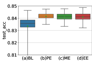
Figure 3: Ensemble method (VGG architecture) versus HASC Accuracy. The number of filters in the first convolutional layer is 16.

From the figure, the ensemble models generally have a higher estimation accuracy than the single model BL, and ME and EE are generally equivalent in terms of estimation accuracy.

4.3 Effects of the model architecture and number of parameters

From Fig. 3, only BL has few trainable parameters under a unified encoder condition. In addition, the model architectures were limited to VGG. We evaluated the effectiveness of various model architectures considering the model size. We implemented ResNet [23], Inception-v3 [29], and SENet [30] (on VGG), which are commonly used as baseline models in image recognition. Each model was modified to EE and other ensemble styles. Fig. 4 shows the change in estimation accuracy with an increase in model size. The results of each model, excluding VGG, were summarized from 50 trials, whereas that of VGG was from 100 trials. The horizontal and vertical axes of Fig. 4, respectively, indicate the number of parameters and estimation accuracy of the test data. Each model was implemented by multiplying the number of filters in each convolutional layer by $x$. Notably, we excluded few results that did not converge ($accuracy(D_{test})\leq 0.5$) and showed the mean and 95% confidence interval in the figure. These results represent the $N=4$ ensembles, and doubling the number of filters in each layer of the BL model is approximately equivalent to the number of parameters in the $N=4$ ensemble model.

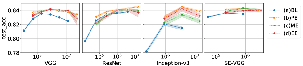
Figure 4: Model size versus HASC accuracy for each model.

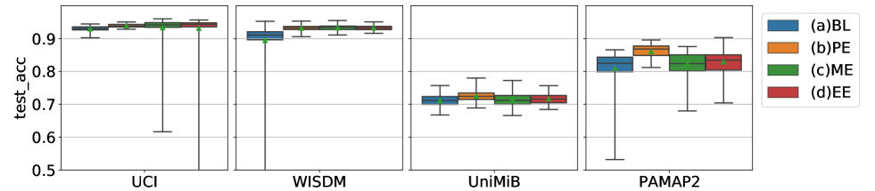
Figure 5: HAR accuracies for each public dataset.

The results of VGG indicated the following four points.

• Under the same model size, ensemble methods outperform BL.

• The accuracy difference among the ensemble methods is not significant; it is approximately $PE\geq ME\simeq EE$.

• Because of the limited size of the training dataset, if the model size becomes too large, the estimation accuracy decreases.

• The changes in the model size and accuracy are generally similar for BL and ensemble methods.

Focusing on other model architectures, the results showed a similar trend to that of VGG, indicating that EE worked well for various model architectures. However, the results also suggested that, in ResNet, EE was sometimes inferior to BL if an appropriate model size was not set. In addition, in Inception-v3, EE outperformed ME, whereas PE outperformed ME and EE in terms of accuracy. We experimentally confirmed the effectiveness of EE; however, it is necessary to consider the theoretical background of this phenomenon in the future.

4.4 Robustness of target domains

In this section, we evaluate the robustness of EE using several public datasets for sensor-based HAR. The additional datasets used were the UCI Smartphone Dataset [31], WISDM [32], UniMiB SHAR [33], and PAMAP2 [4]. Table 1 lists the details of the datasets, including HASC. PAMAP2 has 52 dimensions of sensor data, but we excluded orientation (12 dimensions), which is officially invalid. For the convenience of the process to change the input method described below, we rearranged the order of dimensions and copied only the temperature from one to three dimensions.

Fig. 5 shows the results of a 50-trial experiment; in all datasets, PE outperformed BL, whereas ME and EE were generally equivalent. Moreover, ME and EE were equivalent PE in UCI and WISDM, whereas PE outperformed ME and EE in UniMiB and PAMAP2. One of the characteristics of UniMiB and PAMAP2 is numerous classes, indicating that the effectiveness of ensembles with a single-input single-output model using ME and EE depends on the dataset.

Table 1: Detailed information of datasets

Dataset # of subj. in Shape of train test input output HASC [28] 10 50 (?, 3, 256) (?, 6) UCI Smartphone [31] 21 9 (?, 9, 128) (?, 6) WISDM [32] 26 11 (?, 3, 256) (?, 6) UniMiB SHAR [33] 21 9 (?, 3, 151) (?, 17) PAMAP2 [4] 7 2 (?, 42, 256) (?, 12)

4.5 Considerations for the characteristics of EE

4.5.1 Ablation Study

We conducted an ablation study to investigate the factors that improved the accuracy of EE. Fig. 6 shows 100-trial results. The first letter denotes convolution type (G: group convolution and C: conventional convolution). The second letter denotes normalization type (G: group normalization, L: layer normalization, and B: batch normalization). The third letter denotes the weights of each ensemble path (N: divided by # of ensembles $N$ and 1: divided by 1). As such, CGN is the same as (d) EE and CL1 is the same as (a) BL.

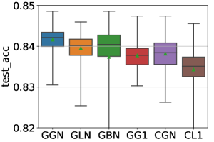
Figure 6: Ablation study (VGG architecture and HASC accuracy). The first letter denotes convolution type (G: group convolution and C: conventional convolution). The second letter denotes normalization type (G: group normalization, L: layer normalization, and B: batch normalization). The third letter denotes the weights of each ensemble path (N: divided by # of ensembles $N$ and 1: divided by 1). CL1 is the same as (a) BL.

We consider Fig. 6 from the viewpoint of ablation study. A 0.5% decrease in accuracy was due to group convolution becoming a conventional convolution (GGN versus CGN) and the lack of $\frac{1}{N}$ when merging ensemble results (GGN versus GG1). In addition, replacing group normalization with layer normalization resulted in a slight decrease in accuracy. The best result was EE (GGN), which incorporated the three factors (group convolution, group normalization, and multiplying $\frac{1}{N}$). The accuracy decreased when group normalization was substituted with batch normalization.

4.5.2 Considerations for the model size and number of ensembles

Fig. 7 shows the accuracy of the HASC (50 trials) when the EE of VGG is scaled up by the number of ensembles $N$. As a comparison, the accuracy of BL scaled up by filter size is shown.

From the figure, the estimation accuracy of the scale-up by filter size reaches its peak around $fil=32$ in BL, whereas the accuracy of the scale-up by the number of ensembles $N$ continues to improve as $N$ increases in PE, ME, and EE. In Fig. 4, EE also tried to scale-up by filter size and showed the same tendency of reaching its peak as BL. Therefore, when tuning the hyperparameters, the best accuracy can be achieved by first determining the filter size with BL and then increasing the number of ensembles $N$, as many as memory allows.

Focusing on the accuracy of PE and EE, the accuracy of PE was greater than or equal to that of EE up to approximately $N\leq 8$, whereas the accuracy of EE exceeded that of PE for $N>8$. Unlike EE, which shares a single loss, it was expected that PE, wherein each path calculates the loss independently, would have higher accuracy; however, when $N$ is large, the results are differ. For PE, each model is trained independently; meanwhile, for EE and ME, each model is treated as a single model, which may yeild to the acquisition of complementary feature representations. This result demonstrates the usefulness of the proposed method.

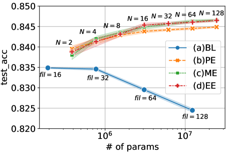
Figure 7: Model Size versus HASC Accuracy. Ensemble models are scaled up by increasing the number of ensembles ($N$).

5 Input variationer

In this section, we propose and evaluate the effectiveness of the input variationer shown in Fig. 1 as a method to add variety to the input given to each group in EE. In ensemble learning, such as bagging, different subsets are assigned to each classifier to obtain diversity. However, so far, we have used the function $R_{N}()$ to repeat the original input ($\bm{X}\in\mathbb{R}^{b\times c\times w}$) $N$ times in the channel direction as $R_{N}(\bm{X})\in\mathbb{R}^{b\times cN\times w}$ to generate the input into EE, where $b$, $c$, and $w$ denote the batch size, number of channels, and window size respectively. In other words, the accuracy of EE can be further improved by diversifying the input because the diversity of EE’s input so far has been given only by the variation in the initial values of network parameters.

5.1 Types of input variationer

The ensemble method using data augmentation (DA) (hereinafter, $A_{N}()$, using the number of ensembles $N$) has been used in several existing studies. For example, in a previous study [34], we proposed a method to ensemble DAs, such as Mixup [35] and RICAP [36], into our original DA method, OctaveMix. In the previous study, DA was fixed for each path; however, in this study, we decided to apply multiple DAs randomly in each path, based on the idea of RandAugment [37]. To formulate, $A_{N}(\bm{X},\bm{t})=cat(t_{i_{0}}(\bm{X}),t_{i_{1}}(\bm{X}),\cdots)$, where $\bm{t}=\{t_{i}|i=0,1,\cdots,N\}$ is a DA set of type i; $i_{0},i_{1},\cdots$ is the index number determined by random numbers without overlap; cat() is the process of combining each tensor in the channel direction.

Another typical method in HAR is a method of training and ensembling the data observed by each sensor modality with independent models [38] (hereinafter, Mod). Notably, the UCI Smartphone Dataset [31] combines total acceleration (3ch), estimated body acceleration (3ch), and angular velocity (3ch) data in the channel direction into nine channels of data. In Mod, when inputting data into EE, no additional processing is required on the DataLoader side, but an appropriate number of groups $N$ must be set on the EE side.

As a new type of input variationer, we propose input masking, which incorporates the idea of bootstrap sampling. In ensemble methods, such as ME and EE, which combine the output parts, it is necessary to handle the input $\bm{X}$ corresponding to the same correct label $\bm{y}$ among the paths of the ensemble to conveniently compute the loss at once. Therefore, in input masking, preparing a mask tensor $\bm{M}\in\mathbb{B}^{b\times N}$ ($\mathbb{B}=\{0,1\}$) in the DataLoader, masked output $\bm{X}_{M}=Mask(\bm{X},\bm{M})=R_{N}(\bm{X})\cdot\bm{M}$ is calculated (Fig. 8). Input masking is a method to construct a pseudosubset of $\bm{X}_{M}$ by masking certain instances of $\bm{X}$ with zeros. The output is $\bm{X}_{M}\in\mathbb{R}^{b\times cN\times w}$. Any method for generating $\bm{M}$ is acceptable; in this study, we assign a random mask as in $N$-fold cross-validation and design the mask such that $N-1$ groups are always valid in each instance. Accordingly, we changed $\frac{1}{N}$ multiplied by the feature map to $\frac{1}{N-1}$.

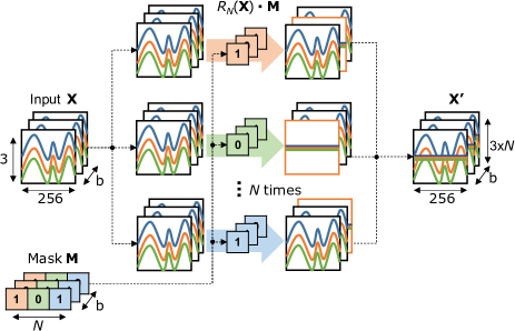
Figure 8: Input masking to make input groups.

5.2 Evaluating input variationer for a single modality dataset

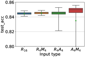
Figure 9: HASC accuracies for each input variation.

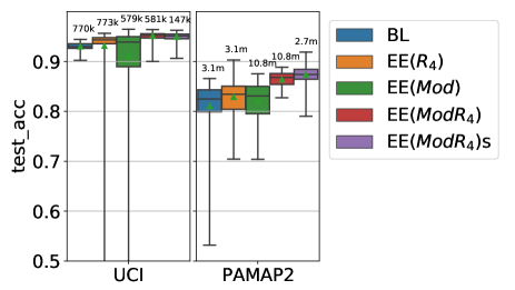
Figure 10: HAR accuracies by modality ensembles (VGG architecture).

First, we evaluated the effectiveness of the input variationer on data measured using a single sensor modality, such as the HASC dataset. The number of ensembles was unified at $N=16$, and combinations of repeat ($R_{N}$), augmentation ($A_{N}$), and input masking ($M_{N}$) were evaluated. Fig. 9 shows the results of 100 trials for each method, where $R_{16}$ denotes the method applying EE with $N=16$, $R_{4}M_{4}$ denotes the method applying input masking with $N=4$ to the repeated input $R_{16}$, $R_{4}A_{4}$ is the method applying augmentation with $N=4$ to $R_{16}$, and $A_{4}M_{4}$ is a method in which $N=4$ times repeats the augmentation result $A_{4}$ and applies input masking of $N=4$. In this study, we adopted four types of DAs: two types of jittering with different magnitudes, scaling of waveform amplitude, and shift in amplitude direction. Notably, rotation was applied in all cases.

As shown in the figure, augmentation ($R_{4}A_{4}$) and input masking ($R_{4}M_{4}$) are equivalent only for repeating ($R_{16}$), but the combination of input masking and augmentation ($A_{4}M_{4}$) succeeds in adding diversity to the input and improves the HAR accuracy by a median of 0.5%. However, there was a tendency for the accuracy to vary, which could be improved additionally using repeat in combination.

5.3 Evaluation of input variationer for multimodality datasets

Next, we evaluated the effect of the input variationer on data measured with multiple modalities, such as UCI and PAMAP2. Fig. 10 shows 50-trial retults using a combination of repeat ($R_{N}$) and modality ensemble ($Mod$). EE($R_{4}$) is EE with repeat for $N=4$, $Mod$ is the modality ensemble, and $ModR_{4}$ is the case where repeat is used with the modality ensemble. Because the number of parameters in $ModR_{4}$ is too large, the number of parameters is adjusted by the filter size in EE($ModR_{4}$)s. The number of parameters for each model is shown in each box plot.

From the figure, the best accuracy was obtained using repeat with modality ensemble for both UCI and PAMAP2. In particular, for PAMAP2, the best accuracy was achieved with lightweight EE ($ModR4$)s, which was lighter than BL and approximately 5% more accurate.

6 Discussion

6.1 Qualitative analysis

Table 2: Qualitative evaluation of ensemble methods.

(a)BL (b)PE (c)ME (d)EE Ease of implementation Good Good Poor Fair Ease of use Good Poor Good Good Model management Good Poor Fair Good Multiple architectures Poor Good Good Poor Stepwise ensemble Poor Fair Fair Good Accuracy Poor Good Good Good

We qualitatively discuss the differences among the ensemble methods. The differences among the four methods discussed in this study are summarized in Table 2. When using BL as the base for implementation, PE is easy to implement because it requires only multiple models, whereas ME requires the input and output parts to be branched and combined. In EE, the input must be coupled in the channel direction, but the output is the same as in BL. In terms of ease of use during training and inference, ME and EE can be used similarly as BL, but PE requires multiple models to be trained and different processes between the training and inference. In terms of model management, such as weight storage, BL and EE only need to manage a single model, whereas PE and ME need to manage multiple models.

The limitation of EE is that various model architectures cannot be ensembled simultaneously: Mukherjee et al. [39] ensembled CNN-Net, Encoded-Net, and CNN-LSTM feature extractors, and Dua et al. [40] ensembled multiple CNN-GRU-based feature extractors with different kernel sizes. Although ensembling feature extractors with various architectures vary feature representations and improve generalization performance, it is time-consuming to implement various architectures. Moreover, although EE can only ensemble the same architectures, it has the advantage of having the number of ensembles $N$ as a hyperparameter, making it easy to implement extended models as a stepwise variation of $N$ among blocks (as described in the next section).

Another advantage of EE is that it allows a single DataLoader and model to divide the roles of the ensemble diversity acquisition. While PE and ME (where the input is not repeated) require the manipulation of multiple DataLoaders, EE requires only a single DataLoader that performs data shaping based on the rule of channel-wise merging. Therefore, users only need to develop a DataLoader for their own dataset and incorporate the input variationer functionality into the DataLoader, which can be reused by simply changing the hyperparameters of the EE model (not requiring the re-development of the model).

In summary, EE is a method that is as easy to use as BL but can benefit from improved accuracy due to its ensemble nature. Compared with PE and ME, EE is easier to implement, and it is easier to implement extensions such as stepwise ensembling.

6.2 Stepwise ensemble

For the five blocks in the VGG architecture, we set all $N=4$ for EE, $\bm{N}=\{4,4.2,2,1\}$ for the EE-D, and $\bm{N}=\{1,2,4,8,16\}$ for the EE-I. Fig. 11 shows the results of 100 trials of ensemble learning, wherein $N$ is varied in steps between blocks. While EE had the best estimation accuracy, EE-I achieved similar accuracy with a model that reduced the number of parameters by approximately 97%. Stepwise ensembling was also discussed in Chen et al.’s study [24]; depending on hyperparameter tuning, this method is expected to provide ensembling benefits with fewer parameters.

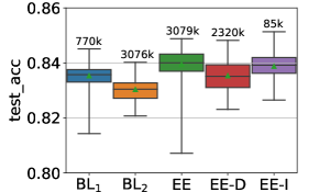
Figure 11: The effect of stepwise ensemble model (HASC acc. and VGG architecture).

7 Conclusion

In this study, we proposed EE as a method that is easy to implement and can be expected to improve accuracy by ensemble learning with a single model. In addition, as input variationer for EE, we proposed repeating input, using DAs, using modality, and masking. After proving that EE is equivalent to ME, which combines the inputs and outputs of multiple models, we experimentally demonstrated its equivalence and effectiveness using a benchmark dataset for sensor-based HAR. Further, we experimentally analyzed the properties of EE and obtained the following.

• When scaled up in terms of the number of filters, the accuracy curves of BL and EE showed roughly the same trend.

• When scaled up in terms of the number of ensembles, the improvement in accuracy tended to continue without an upper limit in the range observed.

• EE tended to outperform PE when the number of ensembles was larger than a certain value.

• Input variationer tended to outperform only input repeating when multiple methods were used together.

In some datasets, PE worked effectively, whereas ME and EE did not. In a future study, we will clarify the conditions under which EE is effective.

References

- [1] C. Xu, D. Chai, J. He, X. Zhang, and S. Duan. Innohar: A deep neural network for complex human activity recognition. IEEE Access, 7:9893–9902, Jan. 2019.
- [2] Jun Long, Wuqing Sun, Zhan Yang, and Osolo Ian Raymond. Asymmetric residual neural network for accurate human activity recognition. Information, 10(6), 2019.
- [3] K. Wang, J. He, and L. Zhang. Attention-based convolutional neural network for weakly labeled human activitiesŕecognition with wearable sensors. IEEE Sensors Journal, 19(17):7598–7604, Sep. 2019.
- [4] A. Reiss and D. Stricker. Creating and benchmarking a new dataset for physical activity monitoring. In In Proc. of the 5th International Conference on PErvasive Technologies Related to Assistive Environments (PETRA), pages 40:1–40:8, 2012.
- [5] Shuochao Yao, Shaohan Hu, Yiran Zhao, Aston Zhang, and Tarek Abdelzaher. Deepsense: A unified deep learning framework for time-series mobile sensing data processing. In Proc. of the 26th International Conference on World Wide Web, page 351–360, 2017.
- [6] Valentin Radu, Catherine Tong, Sourav Bhattacharya, Nicholas D. Lane, Cecilia Mascolo, Mahesh K. Marina, and Fahim Kawsar. Multimodal deep learning for activity and context recognition. Proc. ACM Interact. Mob. Wearable Ubiquitous Technol., 1(4), jan 2018.
- [7] Jun-Ho Choi and Jong-Seok Lee. Embracenet for activity: A deep multimodal fusion architecture for activity recognition. In Adjunct Proc. of the 2019 ACM International Joint Conference on Pervasive and Ubiquitous Computing and Proceedings of the 2019 ACM International Symposium on Wearable Computers, page 693–698, 2019.
- [8] Ling Chen, Xiaoze Liu, Liangying Peng, and Menghan Wu. Deep learning based multimodal complex human activity recognition using wearable devices. Applied Intelligence, 51:4029–4042, jun 2021.
- [9] Abdul Wasay, Brian Hentschel, Yuze Liao, Sanyuan Chen, and Stratos Idreos. Mothernets: Rapid deep ensemble learning. In I. Dhillon, D. Papailiopoulos, and V. Sze, editors, Proc. of Machine Learning and Systems, volume 2, pages 199–215, 2020.
- [10] Abdulhamit Subasi, Dalia H. Dammas, Rahaf D. Alghamdi, Raghad A. Makawi, Eman A. Albiety, Tayeb Brahimi, and Akila Sarirete. Sensor based human activity recognition using adaboost ensemble classifier. Procedia Computer Science, 140:104–111, 2018.
- [11] Naomi Irvine, Chris Nugent, Shuai Zhang, Hui Wang, and Wing W. Y. NG. Neural network ensembles for sensor-based human activity recognition within smart environments. Sensors, 20(1):1–26, 2020.
- [12] Nurul Amin Choudhury, Soumen Moulik, and Diptendu Sinha Roy. Physique-based human activity recognition using ensemble learning and smartphone sensors. IEEE Sensors Journal, 21(15):16852–16860, 2021.
- [13] Shoujiang Xu, Qingfeng Tang, Linpeng Jin, and Zhigeng Pan. A cascade ensemble learning model for human activity recognition with smartphones. Sensors, 19(10):1–17, 2019.
- [14] Ran Zhu, Zhuoling Xiao, Ying Li, Mingkun Yang, Yawen Tan, Liang Zhou, Shuisheng Lin, and Hongkai Wen. Efficient human activity recognition solving the confusing activities via deep ensemble learning. IEEE Access, 7:75490–75499, 2019.
- [15] Anjali Gupta Vijay Bhaskar Semwal and Praveen Lalwani. An optimized hybrid deep learning model using ensemble learning approach for human walking activities recognition. The Journal of Supercomputing, pages 1–25, 2021.
- [16] Stefan Lee, Senthil Purushwalkam, Michael Cogswell, David Crandall, and Dhruv Batra. Why m heads are better than one: Training a diverse ensemble of deep networks, 2015.
- [17] Yeming Wen, Dustin Tran, and Jimmy Ba. Batchensemble: an alternative approach to efficient ensemble and lifelong learning. In Proc. of the International Conference on Learning Representations, 2020.
- [18] Marton Havasi, Rodolphe Jenatton, Stanislav Fort, Jeremiah Zhe Liu, Jasper Snoek, Balaji Lakshminarayanan, Andrew Mingbo Dai, and Dustin Tran. Training independent subnetworks for robust prediction. In Proc. of the International Conference on Learning Representations, 2021.
- [19] Abdul Wasay and Stratos Idreos. More or less: When and how to build convolutional neural network ensembles. In Proc. of the International Conference on Learning Representations, 2021.
- [20] Zeyuan Allen-Zhu and Yuanzhi Li. Towards understanding ensemble, knowledge distillation and self-distillation in deep learning. arXiv, 2012.09816v2:1–70, Jul. 2021.
- [21] Geoffrey Hinton, Oriol Vinyals, and Jeffrey Dean. Distilling the knowledge in a neural network. In Proc. of the NIPS Deep Learning and Representation Learning Workshop, 2015.
- [22] Saining Xie, Ross Girshick, Piotr Dollár, Zhuowen Tu, and Kaiming He. Aggregated residual transformations for deep neural networks. In Proc. of the IEEE Conference on Computer Vision and Pattern Recognition (CVPR), pages 5987–5995, 2017.
- [23] Kaiming He, Xiangyu Zhang, Shaoqing Ren, and Jian Sun. Deep residual learning for image recognition. In Proc. of the IEEE Conference on Computer Vision and Pattern Recognition (CVPR), pages 770–778, 2016.
- [24] Hao Chen and Abhinav Shrivastava. Group ensemble: Learning an ensemble of convnets in a single convnet, 2020.
- [25] K. Simonyan and A. Zisserman. Very deep convolutional networks for large-scale image recognition. In Proc. of the International Conference on Learning Representations, pages 1–14, May 2015.
- [26] François Chollet. Xception: Deep learning with depthwise separable convolutions. In Proc. of the IEEE Conference on Computer Vision and Pattern Recognition (CVPR), pages 1800–1807, 2017.
- [27] Yuxin Wu and Kaiming He. Group normalization. In Proc. of the European Conference on Computer Vision (ECCV), September 2018.
- [28] N. Kawaguchi, N. Ogawa, Y. Iwasaki, K. Kaji, T. Terada, K. Murao, S. Inoue, Y. Kawahara, Y. Sumi, and N. Nishio. Hasc challenge: Gathering large scale human activity corpus for the real-world activity understandings. In In Proc. of the 2nd Augmented Human International Conference, Mar. 2011.
- [29] Christian Szegedy, Vincent Vanhoucke, Sergey Ioffe, Jon Shlens, and Zbigniew Wojna. Rethinking the inception architecture for computer vision. In Proc. of the IEEE Conference on Computer Vision and Pattern Recognition (CVPR), pages 2818–2826, 2016.
- [30] Jie Hu, Li Shen, and Gang Sun. Squeeze-and-excitation networks. In Proc. of the IEEE Conference on Computer Vision and Pattern Recognition (CVPR), June 2018.
- [31] D. Anguita, A. Ghio, L. Oneto, X. Parra, and J. L. Reyes-Ortiz. A public domain dataset for human activity recognition using smartphones. In In Proc. of the 21st European Symposium on Artificial Neural Networks (ESANN), pages 437–442, Apr. 2013.
- [32] J. R. Kwapisz, G. M. Weiss, and S. A. Moore. Activity recognition using cell phone accelerometers. SIGKDD Explor. Newsl., 12(2):74–82, 2011.
- [33] M. Mobilio D. Micucci and P. Napoletano. Unimib shar: A dataset for human activity recognition using acceleration data from smartphones. Apld. Sci.,, 7(10), 2017.
- [34] Tatsuhito Hasegawa. Octave mix: Data augmentation using frequency decomposition for activity recognition. IEEE Access, 9:53679–53686, 2021.
- [35] H. Zhang, M. Cisse, Y. N. Dauphin, and D. Lopez-Paz. mixup: Beyond empirical risk minimization. In Proc. of the International Conference on Learning Representations, pages 1–13, Apr. 2018.
- [36] R. Takahashi, T. Matsubara, and K. Uehara. Ricap: Random image cropping and patchingdata augmentation for deep cnns. In Proc. of Mach. Lrn. Res., volume 95, pages 786–798, Apr. 2018.
- [37] Ekin Dogus Cubuk, Barret Zoph, Jon Shlens, and Quoc Le. Randaugment: Practical automated data augmentation with a reduced search space. In Advances in Neural Information Processing Systems, volume 33, pages 18613–18624, 2020.
- [38] Jessica Sena, Jesimon Barreto, Carlos Caetano, Guilherme Cramer, and William Robson Schwartz. Human activity recognition based on smartphone and wearable sensors using multiscale dcnn ensemble. Neurocomputing, 444:226–243, 2021.
- [39] Debadyuti Mukherjee, Riktim Mondal, Pawan Kumar Singh, Ram Sarkar, and Debotosh Bhattacharjee. Ensemconvnet: a deep learning approach for human activity recognition using smartphone sensors for healthcare applications. Multimedia Tools and Applications, 79:31663–31690, 11 2020.
- [40] Nidhi Dua, Shiva Singh, and Vijay Semwal. Multi-input cnn-gru based human activity recognition using wearable sensors. Computing, 103:1–18, 07 2021.