Sparsification and Filtering for Spatial-temporal GNN in Multivariate Time-series

Abstract.

We propose an end-to-end architecture for multivariate time-series prediction that integrates a spatial-temporal graph neural network with a matrix filtering module. This module generates filtered (inverse) correlation graphs from multivariate time series before inputting them into a GNN. In contrast with existing sparsification methods adopted in graph neural network, our model explicitly leverage time-series filtering to overcome the low signal-to-noise ratio typical of complex systems data. We present a set of experiments, where we predict future sales from a synthetic time-series sales dataset. The proposed spatial-temporal graph neural network displays superior performances with respect to baseline approaches, with no graphical information, and with fully connected, disconnected graphs and unfiltered graphs.

1. Introduction

Multivariate time-series prediction is an important, general, challenge in data science and machine learning. Several deep learning approaches have been proposed in the literature to address multivariate time-series forecasting. However, while they often perform well at extracting temporal patterns, most of the proposed approaches are not designed to account for the interdependency between time-series. Graph neural network, on the other hand, can model time-series as nodes in a graph to account for dependency. Recent development in spatial-temporal graph neural network has been shown to enable multivariate time-series learning and inference (Khodayar and Wang, 2019; Kapoor et al., 2020; Wan et al., 2019).

Applications of multivariate time-series prediction ranges from day-to-day business e.g., sales forecasting, traffic prediction to convoluted topics like bio-statistics and action recognition. It is also one of the cornerstones of modern quantitative finance. At the finest granular level, in finance, modeling the levels of limit order book is a multivariate problem for high-frequency trading with the aim of mid-price prediction (Briola et al., 2020, 2021). For longer-term investment like portfolio management (Markowitz, 1952; Wang and Aste, 2021), prices of assets in a portfolio are usually multivariate time-series. Multivariate time series forecasting methods assume inter-dependencies among dynamically changing variables, which captures systematic trends. Namely, the prediction for each variable not only depends on its historical temporal information, but also the others. Understanding this inter-dependency helps to reveal the underlying dynamics of a larger picture, e.g., the financial market, urban transportation system or the urban distribution of shopping centers. However, its complexity is a key challenge that has been studied for over six decades.

Intra-series temporal patterns and inter-series correlations are jointly the two cores in multivariate time-series forecasting. Recent advancement in deep learning has enabled strong temporal pattern mining. Recurrent Neural Network (RNN) (Rumelhart et al., 1986), Long Short-Term Memory (LSTM) network (Sak et al., 2014), Gated Recurrent Units (GRU) (Chung et al., 2014), Gated Linear Units (GLU) (Dauphin et al., 2017) and Temporal Convolution Networks (TCN) (Bai et al., 2018) demonstrate promising results in temporal modelling. However, existing methods fail to exploit latent inter-dependencies and correlation among time-series. Historical attempts have been made to input covariance/correlation structure into neural network. Matrix-based neural networks have been discussed (Gao et al., 2017; Cai et al., 2006; Daniusis and Vaitkus, 2008), but this approach is not specifically designed for the covariance/correlation matrix, and therefore fails to directly and explicitly address the dependency in the covariance/correlation structure inside the calculation.

Graph is a mathematical structure to model the pairwise relation between objects. The permutation-invariant, local connectivity and compositionality of graphs present a perfect data structure to simulate the correlation/covariance matrix. In fact, network science literature has long been including (sparse) covariance/correlation as a special network for analysis (Chen et al., 2018; Turiel et al., 2020; Procacci and Aste, 2021; Kojaku and Masuda, 2019; Shen et al., 2010), and many network properties of covariance/correlation matrix contribute greatly to analytical and predictive tasks in the financial market (Millington and Niranjan, 2017; Yuan et al., 2020; Lee and Seregina, 2020). Recently, graph neural network (GNN) has been leveraged to incorporate the topology structure between entities. Hence, modeling inter-series correlation via graph learning is a natural extension to analyzing covariance/correlation matrix from a network perspective. Each variable from a multivariate time-series is a node in the graph, and the edge represents their latent inter-dependency. By propagating information between neighboring nodes, the graph neural network enables each time-series to be aware of correlated context.

Spatial-temporal graph neural network is the most used network structure for multivariate time-series problems in the literature (Zhao et al., 2020; Wu et al., 2020; Cao et al., 2020; Sesti et al., 2021), as the temporal part extracts patterns in each uni-variate series with a LSTM/RNN/GRU, while the spatial part (GNN) models the relationship between series with a pre-defined topology or a graph representation learning algorithm. On one hand, existing GNNs heavily utilizes a pre-defined topology structure which is not explicit in multivariate time-series, and does not reflect the temporal dynamics nature of time-series. On the other hand, many graph representation learning methods focus more on generating node embeddings rather than topological structure, and most of the embeddings depend on a pre-defined topological prior or attention mechanism (Ying et al., 2018; Zhao et al., 2020; Franceschi et al., 2019).

In this paper, we propose an end-to-end framework termed Filtered Sparse Spatial-temporal GNN (FSST-GNN) for sales prediction of 50 products in 10 stores. By integrating modern spatial-temporal GNN with traditional matrix filtering/sparsification methods, we demonstrate the direct use of the (inverse) correlation matrix in GNN. Correlation filtering techniques generate a sparse inverse correlation matrix from multivariate time-series, which can be inverted to a filtered correlation matrix. Both the (inverse) correlation can be used as a pre-defined topological structure or prior for further representation learning. With the designed architecture, we further illustrate that filtered graphs generates a positive impact in multivariate time-series learning, and sparse graphs acts as a contributing prior to guide attention mechanism in GNN.

2. Related Works

2.1. Multivariate Time-series Forecasting

Time-series forecasting is one of the long-standing key problems in statistics, data science and machine learning. Techniques ranges from traditional pattern recognition to modern machine learning. Univariate time-series forecasting focuses on analyzing independent time-series by extracting temporal patterns based on historical behaviours, e.g., the moving average (MA), the auto-regressive (AR), the auto-regressive moving average (ARMA) and the autoregressive integrated moving average (ARIMA) (Young and Shellswell, 1972). Modern machine learning model like LSTM has been shown as a good fit to tackle this problem by many literature, e.g., FC-LSTM (Shi et al., 2015) and SMF (Zhang et al., 2017). Multivariate forecasting considers a correlated collection of time-series. The vector auto-regressive model (VAR) and the vector auto-regressive moving average model (VARMA) (Kascha, 2012; Anderson, 1978) extend the aforementioned linear models into a multivariate space by capturing the interdependecy between time-series. Early attempts combines convolution neural network (CNN) and recurrent neural network (RNN) to learn local spatial dependencies and temporal patterns (Lai et al., 2018; Shih et al., 2019). Further works include state space model in Deep-State (Rangapuram et al., 2018) and matrix factorization approach in DeepGLO (Sen et al., 2019).

2.2. Spatial-temporal Graph Neural Network

Spatial-temporal graph neural network has been proposed recently for multivariate time-series problems. To capture the correlation be between time-series in the spatial component, each time-series is modelled as a node in a graph whereas the edge between every two nodes represents their correlation. Early work applies spatial-temporal GNN for traffic forecasting (Li et al., 2018; Yu et al., 2018; Chen et al., 2020; Wu et al., 2019; Zheng et al., 2020). Further studies have been extended to other fields, e.g., action recognition (Shi et al., 2019; Yan et al., 2018) and bio-statistics with many interesting works for COVID-19 (Gatta et al., 2021; Fritz et al., 2021; Kapoor et al., 2020). For financial applications, Matsunaga et al. (Matsunaga et al., 2019) is one of the first studies exploring the idea of incorporating company knowledge graphs directly into the predictive model by GNN. Later, Hou et al. (Hou et al., 2021) proposed to use a variational autoencoder (VAE) to process stock fundamental information and cluster it into graph structure. This learned adjacency matrix is then fed into a GCN-LSTM for further forecasting. Similar work has been done by Pillay & Moodley (Pillay and Moodley, 2022) with a different model architecture called Graph WaveNet. The most recent advancement is a spatial-temporal GNN for portfolio/asset management proposed by Amudi (Pacreau et al., 2021). They combine a stock sector graph, a correlation graph and a supply-chain graph into one super graph and use the multi-head attention in GAT as a sparsification method to select the meaningful subgraph for prediction. In line with this work, we focus on filtered/sparsified (inverse) correlation graph generated from matrix filtering/sparsification techniques.

2.3. Correlation Matrix Filtering

Many computational methods employ sparse approximation techniques to estimate the inverse covariance matrix. The sparsification is effective because the least significant components in a covariance matrix are often largely prone to small changes and can lead to instability. Sparsified models filters out these insignificant components, and thus improve the model resilience to noise. As correlation is a scaled form of covariance, filtering and sparsification methods are equivalently applicable in both cases.

2.3.1. Covariance Shrinkage

A shrinkage algorithm minimizes the ratio between the smallest and the largest eigenvalues of the empirical covariance matrix, which is done by simply shifting every eigenvalue according to a given offset. This approach is equivalent of finding the $L_{2}$-penalized maximum likelihood estimator of the covariance matrix (Ledoit and Wolf, 2003), which is expressed as a simple convex transformation:

(1) $$\Sigma_{\text{shrunk}}=(1-\alpha)\hat{\Sigma}+\alpha\frac{\text{Tr}\hat{\Sigma}}{n}\mathbb{1}$$

where $\Sigma_{\text{shrunk}}$ is the shrunk covariance, $\hat{\Sigma}$ is the empirical covariance, $n$ is the number of features in the covariance, $\mathbb{1}$ is the identity matrix and $\alpha$ is the shrinkage coefficient. To optimise the selection of the shrinkage coefficient, Ledoit and Wolf in 2004 (Ledoit and Wolf, 2004) proposed to compute $\alpha$ that minimizes the mean square error between the estimated and empirical covariance. With further assumption on the normality of data, Chen et al. in 2010 (Chen et al., 2010) proposed a better $\alpha$ computation based on minimum mean square error. Further research focuses on large dimension shrinkage (Ledoit and Wolf, 2012; Donoho et al., 2018; Couillet and Mckay, 2014).

2.3.2. Graphical Models

A widely used approach for inverse covariance estimation is based on graph models. Meinshausen and Buhlmann in 2006 (Meinshausen and Buhlmann, 2006) regards the zero entries in the inverse covariance matrix of a multi-variable normal distribution as conditional independence between variables. These structural zeros can thus be obtained through neighborhood selection with LASSO regression by fitting a LASSO to each variable and using the others as predictors. Similar methods that maximizes $L_{1}$ penalized log-likelihood have been studies by Yuan and Lin (Yuan and Lin, 2007) and Banerjee et al. (Banerjee et al., 2007). In 2008, Friedman et al. (Friedman et al., 2008) developed an efficient Graphical LASSO that uses $L_{1}$ norm regularization to control the sparsity in the precision matrix. The sparse inverse covariance matrix can be obtained through minimizing the regularized negative log-likelihood (Mazumder and Hastie, 2012):

(2) $$\Sigma_{\text{glasso}}^{-1}=\min_{{\mathbf{\Sigma}^{-1}}}(-\log\det{\Sigma^{-1}}+\text{Tr}(\hat{\Sigma}^{-1}\Sigma^{-1})+\lambda||\Sigma^{-1}||_{1})$$

where $\hat{\Sigma}^{-1}$ is the empirical inverse covariance, $||\Sigma^{-1}||_{1}$ denotes the sum of the absolute values of $\Sigma^{-1}$, and $\lambda$ is the regularization constant, optimised by cross-validation.

2.3.3. Information Filtering Network

An alternative approach that uses information filtering networks has been shown to deliver better results with lower computational burden and larger interpretability (Barfuss et al., 2016). In the past few years, information filtering network analysis of complex system data has advanced significantly. It models interactions in a complex system as a network structure of elements (vertices) and interactions (edges). The best-known approach, the Minimum Spanning Tree (MST) was firstly introduced by Boruvka in 1926 (Nešetřil et al., 2001) and it can be solved exactly (see (Kruskal, 1956) and (Prim, 1957) for two common approaches). The MST reduces the structure to a connected tree which retains the larger correlations. To better extract useful information, Tumminello et al. (Tumminello et al., 2005) and Aste and Di Matteo (Aste and Matteo, 2017) introduced the use of planar graphs in the Planar Maximally Filtered Graph (PMFG) algorithm. Recent studies have extended the approach to chordal graphs of flexible sparsity (Massara et al., 2017; Massara and Aste, 2019a). Research fields ranging from finance (Barfuss et al., 2016) to neural systems (Telesford et al., 2011) have applied this approach as a powerful tool to understand high dimensional dependency and construct a sparse representation. It was shown that, for chordal information filtering networks, such as the Triangulated Maximally Filtered Graph (TMFG) (Massara et al., 2017), one can obtain a sparse precision matrix that is positively definite and has the structure of the network paving the way for a proper $L_{0}$-norm topological regularization (Aste, 2020). Further study in Maximally Filtered Clique Forest (MFCF) (Massara and Aste, 2019b) extends the generality of the method by applying it to different sizes of cliques. This approach has proven to be computationally more efficient and stable than Graphical LASSO (Friedman et al., 2008) and covariance shrinkage methods (Ledoit and Wolf, 2003, 2004; Chen et al., 2010), especially when few data points are available (Barfuss et al., 2016; Aste and Matteo, 2017).

2.4. Sparse GNN

Many literature has discussed graph sparsification in GNN. Some, by including regularization, reduce unnecessary edges, which can largely improve the efficiency and efficacy of large-scale graph problems (Calandriello et al., 2018; Chakeri et al., 2016). Some leverage stochastic edge pruning in graphs as a dropout-equivalent regularization to enhance the training process (Rong et al., 2020; Hasanzadeh et al., 2020). Others train the GNN to learn sparsification as an integrated part before applying it to downstream tasks. NeuralSparse learns to sample k-neighbor subgraph as input for GNN (Zheng et al., 2020). Luo proposes to prune task-irrelevant edges (Luo et al., 2021). Kim uses the disconnected edges of sparse graphs to guide attention in GAT (Kim and Oh, 2021).

3. Model Implementation

We first elaborate on the general framework of our model. As illustrated in Figure 1, the model consists of 5 main building blocks. A correlation graph generator is able to transform the multivariate time-series into a correlation graph where each node represents a single time-series and each edge between two nodes denotes their correlation. A standard transformation generates a full (inverse) correlation graph with (inverse) correlation edges between each node. In addition, correlation-filtering based transformation generates a full correlation graph with filtered correlation edges, or a sparse inverse correlation graph. We employ covariance shrinkage, graphical models and information filtering network as the three main correlation-filtering based graph generators. The feature generator generates initial input features for each node based on the multivariate time-series. The generated graph and the features from the two generators are then fed into a GNN to learn meaningful node embeddings as the spatial information. Similarly, the multivariate time-series is also fed into a LSTM to extract temporal information. Then, the spatial and temporal information are input in a multi-layer perceptron (MLP) as the read-out layer for the final output, the predicted sales number.

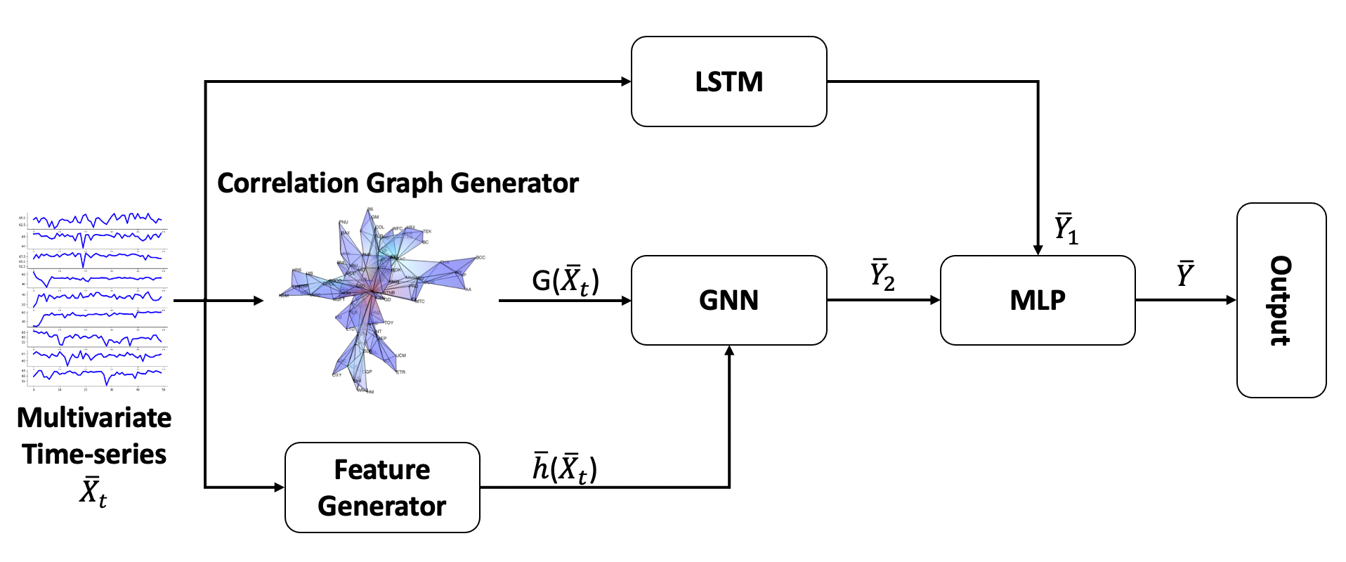
Figure 1. The overall model architecture.

3.1. Correlation Graph Generator

3.1.1. Covariance Shrinkage

Covariance shrinkage method as described in equation 1 is equivalently applicable to the correlation matrix. Shrinkage coefficient $\alpha$ is optimized by cross-validation. There is a implementation, sklearn.covariance.ShrunkCovariance Pyhon library (Pedregosa et al., 2011), which is applied in this experiment. Filtered correlation is then directly transform into a graph. Inverse correlation can be obtained by direct matrix inversion, which is implemented by the numpy.linalg.inv library (Harris et al., 2020).

3.1.2. Graphical LASSO

Graphical LASSO is a graphical model for inverse covariance sparsification, which is epressed in equation 2. We leverage Python’s sklearn.covariance.GraphicalLasso library for implementation, and sklearn.covariance.GraphicalLassoCV (Pedregosa et al., 2011) for cross valiation and regularization constant $\lambda$ selection. Graphical LASSO sparsifies an inverse correlation matrix which can be directly transformed into a sparse inverse correlation graph, while a full but filtered correlation graph can be obtained through the matrix inversion of the inverse correlation.

3.1.3. Maximally Filtered Clique Forest

We implement Maximally Filtered Clique Forest (MFCF), an information filtering network, for sparse precision matrix filtering. By setting the minimum and maximum clique size to 4, we simplify our solution to a TMFG-equivalent model discussed in Section 2.3.3. It generates sparse inverse correlation, which will undergoes similar transformation as Graphical LASSO to obtain inverse correlation and correlation graphs.

3.2. GNN

3.2.1. GCN

Graph convolution network is proposed by Kipf and Welling in 2017 (Kipf and Welling, 2017), which generates embeddings for each node in the graph. It takes original features in each node as the initial embeddings, then aggregates neighboring feature representations and updates the node embeddings through a message-passing like network with the adjacency matrix, which can be expressed as:

(3) $$h_{i}=\sum^{N}_{j}{(\frac{\phi(W^{\top}A_{ij})}{d_{j}})\times h_{j}}$$

where $h_{i}$ is the node embedding, $h_{j}$ is the neighboring node embedding, $W$ is a learnable parameter, $\phi$ is non-linear activation, $A_{ij}$ is the adjacency matrix and $d_{j}$ is the degree of node $j$ for normalization.

In the experiments, we have replaced the graph information, adjacency matrix, expressed in equation 3 by (inverse) correlation matrix, adjacency matrix and Laplacian matrix obtained by thresholding the (inverse) correlation matrix. The empirical results suggest the superiority by simply employing the (inverse) correlation matrix. It can be seen as weighted adjacency matrix, where correlation coefficients are naturally scaled/normalized. Therefore, the graph convolution can be re-expressed as:

(4) $$h_{i}=\sum^{N}_{j}{\phi(W^{\top}C_{ij})\times h_{j}}$$

where $C_{ij}$ is the (inverse) correlation matrix, and all the other parameters are previously defined.

3.2.2. GAT

The implementation of GCN limits the model to be used only with static graphs. The embedding update is static across time, which assumes non-stationarity in time-series. Graph attention network uses masked multi-head attention mechanism to solve this issue by dynamically assigning attention coefficients between nodes. The normalized attention coefficient $a_{ij}$ is computed for nodes $i$ and $j$ based on their features (embeddings):

(5) $$e_{i,j}= a(Wh_{i},Wh_{j})$$

$$= \textrm{LeakyReLU}(\hat{a}^{\top}[Wh_{i}||Wh_{j}])$$

where $W$ is the learnable linear transformation weight matrix to transform node features, $h$, into lower dimensional representations, $a$ is the attention mechanism to perform self-attention on each node and $||$ represents concatenation operation. We normalize the attention coefficient $e_{ij}$ by a softmax function:

(6) $$\alpha_{i,j}= \textrm{softmax}_{j}(e_{i,j})$$

$$= \frac{\exp{e_{i,j}}}{\sum_{k\in\mathcal{N}_{i}}\exp{e_{i,k}}}$$

$$= \frac{\exp{(\textrm{LeakyReLU}(\hat{a}^{\top}[Wh_{i}||Wh_{j}]))}}{\sum_{k\in\mathcal{N}_{i}}\exp{(\textrm{LeakyReLU}(\hat{a}^{\top}[Wh_{i}||Wh_{k}]))}}$$

The multi-head attention mechanism has been proposed by Vaswani et al. (Vaswani et al., 2017) which demonstrates superior and robust performance in network training. GAT incorporates the masked multi-head attention where attention is only computed between neighboring nodes, and the output feature representation is expressed as:

(7) $$h_{i}=\phi(\frac{1}{k}\sum_{k=1}^{K}(\sum_{j\in\mathcal{N}_{i}}\alpha_{i,j}W^{k}h_{j}))$$

where in each level of attention, the representation embedding is updated by a learnable parameter $W$ and the attention coefficient matrix $a_{i,j}$, then the final representation is averaged between the $K$ multi-head attention layers and applied a non-linearity $\phi$.

Graph	Filtering	RMSE	MAE	MAPE
FSST-GNN (GCN)
Cor	Empirical	10.12 $\pm$ 0.53	7.77 $\pm$ 0.39	17.28$\%\pm$1.18$\%$
Cor	Shrinkage	9.99 $\pm$ 0.17	7.72 $\pm$ 0.09	17.34$\%\pm$0.61$\%$
Cor	GLASSO	9.76 $\pm$ 0.47	7.52 $\pm$ 0.39	16.96$\%\pm$1.49$\%$
Cor	MFCF	9.80 $\pm$ 0.61	7.66 $\pm$ 0.43	17.27$\%\pm$1.13$\%$
Inv Cor	Empirical	11.74 $\pm$ 0.99	8.69 $\pm$ 0.46	20.08$\%\pm$0.90$\%$
Inv Cor	Shrinkage	10.59 $\pm$ 1.04	8.26 $\pm$ 0.78	19.15$\%\pm$2.21$\%$
Inv Cor	GLASSO	9.67 $\pm$ 0.41	7.55 $\pm$ 0.34	17.51$\%\pm$1.54$\%$
Inv Cor	MFCF	10.07 $\pm$ 0.59	7.99 $\pm$ 0.44	17.87$\%\pm$1.11$\%$
Zeros	/	13.51 $\pm$ 0.16	10.28 $\pm$ 0.12	22.04$\%\pm$1.01$\%$
Ones	/	12.33 $\pm$ 1.12	10.00 $\pm$ 0.98	24.76$\%\pm$2.33$\%$
Identity	/	11.78 $\pm$ 0.52	9.23 $\pm$ 0.46	21.01$\%\pm$1.78$\%$
LSTM
/	/	16.34 $\pm$ 0.44	12.56 $\pm$ 0.25	26.40$\%\pm$0.98$\%$

Table 1. Summary of forecasting results with different models, graphs and filtering methods. Highlighted in bold are the optimal RMSE, MAE and MAPE in each graph, and underlined is the absolute optimal results in the table. A LSTM results is attached as the baseline.

4. Experiments

4.1. Setup

We test our model on a Kaggle playground code competition, Store Item Demand Forecasting Challenge (Kaggle, [n.d.]). The dataset consists of 5-year sales time-series data of 50 products in 10 different stores. For simplicity, we re-formulate the problem as 50 mini-problems, each focuses on 1 product in 10 different stores. At each time-stamp, the temporal component regresses each of the 10 time-series individually based on its historical value. The dependency between them is reflected by the final embeddings generated from the spatial component. The outputs from each component are subsequently concatenated and, by a read-out layer, to generate final daily forecasting for the product. We assume stationarity in the time-series, therefore, we separate the training and testing data as the 80% and 20% of the raw dataset.

The temporal component of the FSST-GNN is a LSTM, which has an input size of ($t_{lb}$, 10) where $t_{lb}=14$ is the look back window size of historical sales, and 10 is the number of different stores. The feature generator produces node features (initial embeddings). We employ the four moments (mean, standard deviation, skewness and kurtosis) of the sales time-series distribution based on each 14-day look back window. The correlation graph generator generates a graph with edge represents the correlation between any two of the 14-day sample time-series in the 10 stores. Then, the generated node features and edges are input into the GNN. In the experiments, a GCN and a GAT have been used as the spatial component.

To understand the effect of filtering and sparsification for multivariate time-series graph learning, we perform 4 sets of experiment: 1) FSST-GNN (GCN) on different filtered correlation graphs; 2) FSST-GNN (GCN) on different filtered inverse correlation graphs; 3) FSST-GNN (GCN) on GLASSO-filtered and MFCF-filtered inverse correlation graph with different levels of sparsity; and 4) FSST-GNN (GAT) on GLASSO-filtered and MFCF-filtered inverse correlation graph with different levels of sparsity. Each experiment has been re-computed 10 times with different random seeds, and the final results is averaged for statistical robustness.

Sparsity	RMSE	MAE	MAPE	Sparsity	RMSE	MAE	MAPE
GLASSO				MFCF
77.2%	10.24 $\pm$ 0.61	8.03$\pm$ 0.47	18.89$\%\pm$1.35$\%$	76.6%	11.35 $\pm$ 0.76	8.76 $\pm$ 0.61	20.36$\%\pm$1.97$\%$
71.0%	10.34 $\pm$ 0.79	8.05 $\pm$ 0.58	18.66$\%\pm$1.29$\%$	72.3%	10.23 $\pm$ 0.26	8.06 $\pm$ 0.44	18.13$\%\pm$1.14$\%$
66.6%	9.80 $\pm$ 0.41	7.66 $\pm$ 0.33	17.75$\%\pm$0.87$\%$	68.6%	10.68 $\pm$ 0.80	8.32 $\pm$ 0.52	19.56$\%\pm$1.30$\%$
60.0%	9.67 $\pm$ 0.41	7.55 $\pm$ 0.34	17.51$\%\pm$1.54$\%$	61.3%	10.07 $\pm$ 0.59	7.99 $\pm$ 0.44	17.87$\%\pm$1.11$\%$
56.5%	9.86 $\pm$ 0.58	7.74 $\pm$ 0.53	18.24$\%\pm$1.66$\%$	58.0%	10.19 $\pm$ 0.41	8.12 $\pm$ 0.29	18.29$\%\pm$0.49$\%$
51.3%	10.06 $\pm$ 0.57	7.86 $\pm$ 0.45	17.68$\%\pm$1.20$\%$	54.8%	10.31 $\pm$ 0.52	8.09 $\pm$ 0.39	18.22$\%\pm$1.26$\%$
43.3%	9.99 $\pm$ 0.27	7.88 $\pm$ 0.19	17.60$\%\pm$0.47$\%$	43.7%	10.75 $\pm$ 0.68	8.16 $\pm$ 0.40	18.44$\%\pm$0.55$\%$

Table 2. Summary of forecasting results of FSST-GNN (GCN) with different filtering methods and sparsity on inverse correlation graph. Highlighted in bold are the optimal RMSE, MAE and MAPE in each model-sparsity combination, and underlined is the absolute optimal results in the table.

Sparsity	RMSE	MAE	MAPE	Sparsity	RMSE	MAE	MAPE
GLASSO				MFCF
77.2%	9.88 $\pm$ 0.59	7.58 $\pm$ 0.43	16.17$\%\pm$0.53$\%$	76.6%	10.47 $\pm$ 0.75	8.09 $\pm$ 0.68	17.61$\%\pm$2.64$\%$
71.0%	10.03 $\pm$ 0.65	7.73 $\pm$ 0.52	16.56$\%\pm$1.07$\%$	72.3%	10.27 $\pm$ 0.62	7.86 $\pm$ 0.46	17.24$\%\pm$0.99$\%$
66.6%	9.63 $\pm$ 0.36	7.42 $\pm$ 0.25	15.82$\%\pm$0.25$\%$	68.6%	9.90 $\pm$ 1.17	7.60 $\pm$ 0.95	16.01$\%\pm$1.78$\%$
60.0%	9.58 $\pm$ 0.31	7.37 $\pm$ 0.20	15.62$\%\pm$0.26$\%$	61.3%	9.46 $\pm$ 0.68	7.31 $\pm$ 0.45	15.44$\%\pm$0.19$\%$
56.5%	9.64 $\pm$ 0.34	7.41 $\pm$ 0.23	15.80$\%\pm$0.47$\%$	58.0%	9.65 $\pm$ 0.46	7.53 $\pm$ 0.32	15.63$\%\pm$0.54$\%$
51.3%	9.75 $\pm$ 0.33	7.55 $\pm$ 0.31	17.28$\%\pm$1.18$\%$	54.8%	9.81 $\pm$ 0.53	7.53 $\pm$ 0.37	16.03$\%\pm$0.54$\%$
43.3%	10.12 $\pm$ 0.53	7.77 $\pm$ 0.39	17.28$\%\pm$1.18$\%$	43.7%	9.90 $\pm$ 0.38	7.63 $\pm$ 0.30	16.31$\%\pm$0.92$\%$

Table 3. Summary of forecasting results of FSST-GNN (GAT) with different filtering methods and sparsity on inverse correlation graph. Highlighted in bold are the optimal RMSE, MAE and MAPE in each model-sparsity combination, and underlined is the absolute optimal results in the table.

4.2. Results

We compute the root mean square error (RMSE), mean average error (MAE) and mean average percentage error (MAPE) of the predicted sales number of all 50 products in 10 stores with the ground truth label in Table 1 as the evaluation matrix to analyze the effectiveness of filtering methods over FSST-GNN with GCN on the correlation and inverse correlation graph respectively. Since all filtering methods are parametric, the table reports the optimal results from covariance shrinkage (Shrinkage), graphical LASSO (GLASSO) and MFCF, which are obtained through grid-search. We also include a fully connected graph of a matrix of ones, two fully disconnected graphs of a matrix of zeros and an identity matrix as benchmarks for comparison. In addition, a plain LSTM is also presented as the baseline model where no graphical/spatial information is input.

In Table 1, it is evident that all FSST-GNN (GCN) outperforms the plain LSTM, which confirms the efficacy of considering the spatial information in multivariate time-series problems. Other benchmarks of fully connected/disconnected graphs are also presented, and their results in all three measurements are effectively inferior to any (inverse) correlation based graph methods. These results further assert the information gain from meaningful spatial graphs.

Highlighted in each column of Table 1 are the best results in first two experiment: 1) FSST-GNN (GCN) on correlation graph; 2) FSST-GNN (GCN) on inverse correlation graph. In correlation graph cases, a filtered correlation graphs demonstrate superior results than the original Empirical correlation graph. Both MFCF and GLASSO filtering are operated on the inverse correlation for sparsification, and then inverted back to a full correlation graphs, while Shrinkage operates directly on correlation. Therefore, the superior results in MFCF and GLASSO than Shrinkage may suggest a stronger filtering effect behind graph/network-based methods, and inversion does not affect filtering.

To understand the effect in filtering and sparsification, results from the same setup with inverse correlation graphs are compared, where full and Shrinkage-filtered inverse correlation graphs are full graphs and GLASSO-filtered and MFCF-filtered graphs are sparse graphs. In this case, Shrinkage filters a correlation and inverts it to an inverse correlation. Comparably to the correlation graph case, Shrinkage consistently yields better result than the Empirical, which further validates that the filtering mechanism is hardly impacted by inversion operation. Furthermore, we observe even more significant results from two sparse graphs filtered by GLASSO and MFCF. This advantage could possibly come from both the filtering, the sparsification, as well as their combined effect. To further investigate the sole efficacy of sparsification, we perform the third and fourth sets of experiments: 3) FSST-GNN (GCN) on GLASSO-filtered and MFCF-filtered inverse correlation graph with different levels of sparsity; and 4) FSST-GNN (GAT) on GLASSO-filtered and MFCF-filtered inverse correlation graph with different levels of sparsity.

Presented in Table 2 and Table 3 are the results with different levels of sparsity. We select the parameter to match the sparsity level between GLASSO and MFCF for comparison. It is seen that at around $60\%$ sparsity, the highlighted best results are achieved for both MFCF and GLASSO in FSST-GNN (GCN) and FSST-GNN (GAT) models. Moreover, as the sparsity deviates away from this local minimum, the three errors start to increase, which may suggest an optimal sparsity structure of the inverse correlation graph in our experimental case. In addition, this optimal structure is independent of the chosen model. Furthermore, as illustrated in equation 7, GAT by default does not account for edge weights in weighted graphs (correlation graphs) as GCN. Hence, the sparse inverse correlation graph serves as a thresholded adjacency matrix, where 0 entries are interpreted as disconnection between nodes. Then, attention, which is only calculated between linked nodes, acts as the edge weights. Namely, the superior performance in Table 2 is a mixture of filtering and sparsity, but the performance in Table 3 is merely determined by the sparsity of the input graph without filtering mechanism.

5. Conclusion

Literature has presented many GNN-based graph sparsification methods. However, none of them explicitly addresses the filtering and sparsification from a time-series perspective. In small sample time-series problems, especially in finance, graph structure learning models, e.g., graph representation learning, are highly prone to noise. In this paper, we design an end-to-end filtered sparse spatial-temporal graph neural network for time-series forecasting. Our model leverages and integrates traditional matrix filtering methods with modern graph neural networks to achieve robust results, and show the use of a simple and efficient architecture. We employ three different matrix filtering methods, covariance shrinkage, graphical LASSO and information filtering network-maximally filtered clique forest to show a positive gain in graph filtering to graph learning. The results from the three methods surpass all of the benchmark approaches, including a LSTM with no graphical information, the same FSST-GNN architecture with fully connected, disconnected graphs and unfiltered graphs.

In the experiments, we found the sparse graph in GAT serves only as an indication of which pairs of node require attention calculation, and the advantages from sparsity are significant. The filtered correlation matrix in GCN is interpreted and used as a weighted adjacency matrix for direct graph convolution, where the efficacy of filtering is also obvious. Furthermore, the optimal combined effect of filtering and sparsification in FSST-GNN (GCN) with inverse correlation implies the two contributing factors are complementary. Therefore, by incorporating weighted graphs in GAT like Grassia & Mangioni (Grassia and Mangioni, 2022), we may further improve the performance of attention-based graph neural networks.

Current work is based on a synthetic dataset from a Kaggle competition for sales prediction. Further work will be applied with real world financial data for practical problems, e.g., portfolio optimization, risk management and price forecasting. The temporal and spatial component of the current architecture are designed to compute in parallel and combined in the end. Therefore, temporal information does not directly contribute to the spatial filtered graph generation or graph node feature generation. In the next phase of this study, we aim to develop a stacked architecture, where temporal signals contribute to spatial graph filtering/sparsification.

References

- (1)
- Anderson (1978) Theodore W. Anderson. 1978. Maximum Likelihood Estimation for Vector Autoregressive Moving Average Models.
- Aste (2020) Tomaso Aste. 2020. Topological regularization with information filtering networks. arXiv preprint arXiv:2005.04692 (2020).
- Aste and Matteo (2017) T. Aste and T. Matteo. 2017. Sparse Causality Network Retrieval from Short Time Series. Complex. 2017 (2017), 4518429:1–4518429:13.
- Bai et al. (2018) Shaojie Bai, J. Zico Kolter, and Vladlen Koltun. 2018. An Empirical Evaluation of Generic Convolutional and Recurrent Networks for Sequence Modeling. ArXiv abs/1803.01271 (2018).
- Banerjee et al. (2007) Onureena Banerjee, Laurent El Ghaoui, and Alexandre d’Aspremont. 2007. Model Selection Through Sparse Maximum Likelihood Estimation. ArXiv abs/0707.0704 (2007).
- Barfuss et al. (2016) Wolfram Barfuss, Guido Previde Massara, T. Di Matteo, and Tomaso Aste. 2016. Parsimonious modeling with information filtering networks. Physical Review E 94, 6 (Dec 2016). https://doi.org/10.1103/physreve.94.062306
- Briola et al. (2020) Antonio Briola, Jeremy D. Turiel, and Tomaso Aste. 2020. Deep Learning Modeling of the Limit Order Book: A Comparative Perspective. ERN: Other Econometrics: Econometric & Statistical Methods - Special Topics (Topic) (2020).
- Briola et al. (2021) Antonio Briola, Jeremy D. Turiel, Riccardo Marcaccioli, and Tomaso Aste. 2021. Deep Reinforcement Learning for Active High Frequency Trading. ArXiv abs/2101.07107 (2021).
- Cai et al. (2006) Deng Cai, Xiaofei He, and Jiawei Han. 2006. Learning with Tensor Representation.
- Calandriello et al. (2018) Daniele Calandriello, Ioannis Koutis, Alessandro Lazaric, and Michal Valko. 2018. Improved Large-Scale Graph Learning through Ridge Spectral Sparsification. In ICML.
- Cao et al. (2020) Defu Cao, Yujing Wang, Juanyong Duan, Ce Zhang, Xia Zhu, Congrui Huang, Yunhai Tong, Bixiong Xu, Jing Bai, Jie Tong, and Qi Zhang. 2020. Spectral Temporal Graph Neural Network for Multivariate Time-series Forecasting. ArXiv abs/2103.07719 (2020).
- Chakeri et al. (2016) Alireza Chakeri, Hamidreza Farhidzadeh, and Lawrence O. Hall. 2016. Spectral sparsification in spectral clustering. 2016 23rd International Conference on Pattern Recognition (ICPR) (2016), 2301–2306.
- Chen et al. (2018) Shuo Chen, Jian Kang, Yishi Xing, Yunpeng Zhao, and Don Milton. 2018. Estimating large covariance matrix with network topology for high-dimensional biomedical data. Comput. Stat. Data Anal. 127 (2018), 82–95.
- Chen et al. (2020) Weiqiu Chen, Ling Chen, Yu Xie, Wei Cao, Yusong Gao, and Xiaojie Feng. 2020. Multi-Range Attentive Bicomponent Graph Convolutional Network for Traffic Forecasting. ArXiv abs/1911.12093 (2020).
- Chen et al. (2010) Yilun Chen, Ami Wiesel, Yonina C. Eldar, and Alfred O. Hero. 2010. Shrinkage Algorithms for MMSE Covariance Estimation. IEEE Transactions on Signal Processing 58 (2010), 5016–5029.
- Chung et al. (2014) Junyoung Chung, Çaglar Gülçehre, Kyunghyun Cho, and Yoshua Bengio. 2014. Empirical Evaluation of Gated Recurrent Neural Networks on Sequence Modeling. ArXiv abs/1412.3555 (2014).
- Couillet and Mckay (2014) Romain Couillet and Matthew R. Mckay. 2014. Large dimensional analysis and optimization of robust shrinkage covariance matrix estimators. J. Multivar. Anal. 131 (2014), 99–120.
- Daniusis and Vaitkus (2008) Povilas Daniusis and Pranas Vaitkus. 2008. Neural Network with Matrix Inputs. Informatica 19 (2008), 477–486.
- Dauphin et al. (2017) Yann Dauphin, Angela Fan, Michael Auli, and David Grangier. 2017. Language Modeling with Gated Convolutional Networks. In ICML.
- Donoho et al. (2018) David L. Donoho, Matan Gavish, and Iain M. Johnstone. 2018. Optimal Shrinkage of Eigenvalues in the Spiked Covariance Model. Annals of statistics 46 4 (2018), 1742–1778.
- Franceschi et al. (2019) Jean-Yves Franceschi, Aymeric Dieuleveut, and Martin Jaggi. 2019. Unsupervised Scalable Representation Learning for Multivariate Time Series. In NeurIPS.
- Friedman et al. (2008) J. Friedman, T. Hastie, and R. Tibshirani. 2008. Sparse inverse covariance estimation with the graphical lasso. Biostatistics 9 3 (2008), 432–41.
- Fritz et al. (2021) Cornelius Fritz, Emilio Dorigatti, and D. Rügamer. 2021. Combining Graph Neural Networks and Spatio-temporal Disease Models to Predict COVID-19 Cases in Germany. ArXiv abs/2101.00661 (2021).
- Gao et al. (2017) Junbin Gao, Yi Guo, and Zhiyong Wang. 2017. Matrix Neural Networks. ArXiv abs/1601.03805 (2017).
- Gatta et al. (2021) Valerio La Gatta, Vincenzo Moscato, Marco Postiglione, and Giancarlo Sperlí. 2021. An Epidemiological Neural Network Exploiting Dynamic Graph Structured Data Applied to the COVID-19 Outbreak. IEEE Transactions on Big Data 7 (2021), 45–55.
- Grassia and Mangioni (2022) Marco Grassia and Giuseppe Mangioni. 2022. wsGAT: Weighted and Signed Graph Attention Networks for Link Prediction. ArXiv abs/2109.11519 (2022).
- Harris et al. (2020) Charles R. Harris, K. Jarrod Millman, Stéfan J van der Walt, Ralf Gommers, Pauli Virtanen, David Cournapeau, Eric Wieser, Julian Taylor, Sebastian Berg, Nathaniel J. Smith, Robert Kern, Matti Picus, Stephan Hoyer, Marten H. van Kerkwijk, Matthew Brett, Allan Haldane, Jaime Fernández del Río, Mark Wiebe, Pearu Peterson, Pierre Gérard-Marchant, Kevin Sheppard, Tyler Reddy, Warren Weckesser, Hameer Abbasi, Christoph Gohlke, and Travis E. Oliphant. 2020. Array programming with NumPy. Nature 585 (2020), 357–362. https://doi.org/10.1038/s41586-020-2649-2
- Hasanzadeh et al. (2020) Arman Hasanzadeh, Ehsan Hajiramezanali, Shahin Boluki, Mingyuan Zhou, Nick G. Duffield, Krishna R. Narayanan, and Xiaoning Qian. 2020. Bayesian Graph Neural Networks with Adaptive Connection Sampling. ArXiv abs/2006.04064 (2020).
- Hou et al. (2021) Xiurui Hou, Kai Wang, Cheng Zhong, and Zhi Wei. 2021. ST-Trader: A Spatial-Temporal Deep Neural Network for Modeling Stock Market Movement. IEEE/CAA Journal of Automatica Sinica 8 (2021), 1015–1024.
- Kaggle ([n.d.]) Kaggle. [n.d.]. Kaggle: Store Item Demand Forecasting Challenge. https://www.kaggle.com/c/demand-forecasting-kernels-only/data. Accessed: 2022-02-06.
- Kapoor et al. (2020) Amol Kapoor, Xue Ben, Luyang Liu, Bryan Perozzi, Matt Barnes, Martin J. Blais, and Shawn O’Banion. 2020. Examining COVID-19 Forecasting using Spatio-Temporal Graph Neural Networks. ArXiv abs/2007.03113 (2020).
- Kascha (2012) Christian Kascha. 2012. A Comparison of Estimation Methods for Vector Autoregressive Moving-Average Models. Econometric Reviews 31 (2012), 297 – 324.
- Khodayar and Wang (2019) Mahdi Khodayar and Jianhui Wang. 2019. Spatio-Temporal Graph Deep Neural Network for Short-Term Wind Speed Forecasting. IEEE Transactions on Sustainable Energy 10 (2019), 670–681.
- Kim and Oh (2021) Dongkwan Kim and Alice H. Oh. 2021. How to Find Your Friendly Neighborhood: Graph Attention Design with Self-Supervision. In ICLR.
- Kipf and Welling (2017) Thomas Kipf and Max Welling. 2017. Semi-Supervised Classification with Graph Convolutional Networks. ArXiv abs/1609.02907 (2017).
- Kojaku and Masuda (2019) Sadamori Kojaku and Naoki Masuda. 2019. Constructing networks by filtering correlation matrices: a null model approach. Proceedings of the Royal Society A 475 (2019).
- Kruskal (1956) Joseph B. Kruskal. 1956. On the shortest spanning subtree of a graph and the traveling salesman problem.
- Lai et al. (2018) Guokun Lai, Wei-Cheng Chang, Yiming Yang, and Hanxiao Liu. 2018. Modeling Long- and Short-Term Temporal Patterns with Deep Neural Networks. The 41st International ACM SIGIR Conference on Research & Development in Information Retrieval (2018).
- Ledoit and Wolf (2003) Olivier Ledoit and Michael Wolf. 2003. Honey, I Shrunk the Sample Covariance Matrix. Capital Markets: Asset Pricing & Valuation (2003).
- Ledoit and Wolf (2004) Olivier Ledoit and Michael Wolf. 2004. A well-conditioned estimator for large-dimensional covariance matrices. Journal of Multivariate Analysis 88 (2004), 365–411.
- Ledoit and Wolf (2012) Olivier Ledoit and Michael Wolf. 2012. Nonlinear shrinkage estimation of large-dimensional covariance matrices. arXiv: Statistics Theory (2012).
- Lee and Seregina (2020) Tae-Hwy Lee and Ekaterina Seregina. 2020. Optimal Portfolio Using Factor Graphical Lasso. arXiv: Econometrics (2020).
- Li et al. (2018) Yaguang Li, Rose Yu, Cyrus Shahabi, and Yan Liu. 2018. Diffusion Convolutional Recurrent Neural Network: Data-Driven Traffic Forecasting. arXiv: Learning (2018).
- Luo et al. (2021) Dongsheng Luo, Wei Cheng, Wenchao Yu, Bo Zong, Jingchao Ni, Haifeng Chen, and Xiang Zhang. 2021. Learning to Drop: Robust Graph Neural Network via Topological Denoising. Proceedings of the 14th ACM International Conference on Web Search and Data Mining (2021).
- Markowitz (1952) H. Markowitz. 1952. Portfolio Selection. The Journal of Finance 7, 1 (1952).
- Massara and Aste (2019a) Guido Previde Massara and Tomaso Aste. 2019a. Learning Clique Forests. ArXiv 1905.02266 (2019).
- Massara and Aste (2019b) Guido Previde Massara and Tomaso Aste. 2019b. Learning Clique Forests. ArXiv abs/1905.02266 (2019).
- Massara et al. (2017) Guido Previde Massara, T. Matteo, and T. Aste. 2017. Network Filtering for Big Data: Triangulated Maximally Filtered Graph. ArXiv abs/1505.02445 (2017).
- Matsunaga et al. (2019) Daiki Matsunaga, Toyotaro Suzumura, and Toshihiro Takahashi. 2019. Exploring Graph Neural Networks for Stock Market Predictions with Rolling Window Analysis. ArXiv abs/1909.10660 (2019).
- Mazumder and Hastie (2012) Rahul Mazumder and Trevor J. Hastie. 2012. The Graphical Lasso: New Insights and Alternatives. Electronic journal of statistics 6 (2012), 2125–2149.
- Meinshausen and Buhlmann (2006) Nicolai Meinshausen and Peter Buhlmann. 2006. High-dimensional graphs and variable selection with the Lasso. Annals of Statistics 34 (2006), 1436–1462.
- Millington and Niranjan (2017) Tristan Millington and Mahesan Niranjan. 2017. Robust Portfolio Risk Minimization Using the Graphical Lasso. In ICONIP.
- Nešetřil et al. (2001) Jaroslav Nešetřil, Eva Milková, and Helena Nešetřilová. 2001. Otakar Boruvka on minimum spanning tree problem Translation of both the 1926 papers, comments, history. Discrete mathematics 233, 1-3 (2001), 3–36.
- Pacreau et al. (2021) Grégoire Pacreau, Edmond Lezmi, and Jiali Xu. 2021. Graph Neural Networks for Asset Management. SSRN (2021).
- Pedregosa et al. (2011) F. Pedregosa, G. Varoquaux, A. Gramfort, V. Michel, B. Thirion, O. Grisel, M. Blondel, P. Prettenhofer, R. Weiss, V. Dubourg, J. Vanderplas, A. Passos, D. Cournapeau, M. Brucher, M. Perrot, and E. Duchesnay. 2011. Scikit-learn: Machine Learning in Python. Journal of Machine Learning Research 12 (2011), 2825–2830.
- Pillay and Moodley (2022) Kialan Pillay and Deshendran Moodley. 2022. Exploring Graph Neural Networks for Stock Market Prediction on the JSE. Artificial Intelligence Research (2022).
- Prim (1957) Robert C. Prim. 1957. Shortest connection networks and some generalizations. Bell System Technical Journal 36 (1957), 1389–1401.
- Procacci and Aste (2021) Pier Francesco Procacci and Tomaso Aste. 2021. Forecasting market states. Machine Learning and AI in Finance (2021).
- Rangapuram et al. (2018) Syama Sundar Rangapuram, Matthias W. Seeger, Jan Gasthaus, Lorenzo Stella, Bernie Wang, and Tim Januschowski. 2018. Deep State Space Models for Time Series Forecasting. In NeurIPS.
- Rong et al. (2020) Yu Rong, Wen bing Huang, Tingyang Xu, and Junzhou Huang. 2020. DropEdge: Towards Deep Graph Convolutional Networks on Node Classification. In ICLR.
- Rumelhart et al. (1986) David E. Rumelhart, Geoffrey E. Hinton, and Ronald J. Williams. 1986. Learning internal representations by error propagation.
- Sak et al. (2014) Hasim Sak, Andrew W. Senior, and Françoise Beaufays. 2014. Long short-term memory recurrent neural network architectures for large scale acoustic modeling. In INTERSPEECH.
- Sen et al. (2019) Rajat Sen, Hsiang-Fu Yu, and Inderjit S. Dhillon. 2019. Think Globally, Act Locally: A Deep Neural Network Approach to High-Dimensional Time Series Forecasting. In NeurIPS.
- Sesti et al. (2021) Nathan Sesti, Juan Jose Garau Luis, Edward F. Crawley, and Bruce G. Cameron. 2021. Integrating LSTMs and GNNs for COVID-19 Forecasting. ArXiv abs/2108.10052 (2021).
- Shen et al. (2010) Huawei Shen, Xue qi Cheng, and Bin xing Fang. 2010. Covariance, correlation matrix, and the multiscale community structure of networks. Physical review. E, Statistical, nonlinear, and soft matter physics 82 1 Pt 2 (2010), 016114.
- Shi et al. (2019) Lei Shi, Yifan Zhang, Jian Cheng, and Hanqing Lu. 2019. Two-Stream Adaptive Graph Convolutional Networks for Skeleton-Based Action Recognition. 2019 IEEE/CVF Conference on Computer Vision and Pattern Recognition (CVPR) (2019), 12018–12027.
- Shi et al. (2015) Xingjian Shi, Zhourong Chen, Hao Wang, Dit-Yan Yeung, Wai-Kin Wong, and Wang chun Woo. 2015. Convolutional LSTM Network: A Machine Learning Approach for Precipitation Nowcasting. In NIPS.
- Shih et al. (2019) Shun-Yao Shih, Fan-Keng Sun, and Hung yi Lee. 2019. Temporal pattern attention for multivariate time series forecasting. Machine Learning (2019), 1–21.
- Telesford et al. (2011) Qawi K. Telesford, S. Simpson, J. Burdette, S. Hayasaka, and P. Laurienti. 2011. The Brain as a Complex System: Using Network Science as a Tool for Understanding the Brain. Brain connectivity 1 (4) (2011), 295–308.
- Tumminello et al. (2005) M. Tumminello, T. Aste, T. Di Matteo, and R. N. Mantegna. 2005. A tool for filtering information in complex systems. Proceedings of the National Academy of Sciences 102, 30 (2005), 10421–10426. https://doi.org/10.1073/pnas.0500298102 arXiv:https://www.pnas.org/content/102/30/10421.full.pdf
- Turiel et al. (2020) Jeremy D. Turiel, Paolo Barucca, and Tomaso Aste. 2020. Simplicial persistence of financial markets: filtering, generative processes and portfolio risk. arXiv: Statistical Finance (2020).
- Vaswani et al. (2017) Ashish Vaswani, Noam M. Shazeer, Niki Parmar, Jakob Uszkoreit, Llion Jones, Aidan N. Gomez, Lukasz Kaiser, and Illia Polosukhin. 2017. Attention is All you Need. ArXiv abs/1706.03762 (2017).
- Wan et al. (2019) Renzhuo Wan, Shuping Mei, Jun Wang, Min Liu, and F. Yang. 2019. Multivariate Temporal Convolutional Network: A Deep Neural Networks Approach for Multivariate Time Series Forecasting. Electronics (2019).
- Wang and Aste (2021) Yuanrong Wang and Tomaso Aste. 2021. Dynamic Portfolio Optimization with Inverse Covariance Clustering.
- Wu et al. (2020) Zonghan Wu, Shirui Pan, Guodong Long, Jing Jiang, Xiaojun Chang, and Chengqi Zhang. 2020. Connecting the Dots: Multivariate Time Series Forecasting with Graph Neural Networks. Proceedings of the 26th ACM SIGKDD International Conference on Knowledge Discovery & Data Mining (2020).
- Wu et al. (2019) Zonghan Wu, Shirui Pan, Guodong Long, Jing Jiang, and Chengqi Zhang. 2019. Graph WaveNet for Deep Spatial-Temporal Graph Modeling. In IJCAI.
- Yan et al. (2018) Sijie Yan, Yuanjun Xiong, and Dahua Lin. 2018. Spatial Temporal Graph Convolutional Networks for Skeleton-Based Action Recognition. ArXiv abs/1801.07455 (2018).
- Ying et al. (2018) Rex Ying, Jiaxuan You, Christopher Morris, Xiang Ren, William L. Hamilton, and Jure Leskovec. 2018. Hierarchical Graph Representation Learning with Differentiable Pooling. ArXiv abs/1806.08804 (2018).
- Young and Shellswell (1972) P. J. Young and Stephen Shellswell. 1972. Time series analysis, forecasting and control. IEEE Trans. Automat. Control 17 (1972), 281–283.
- Yu et al. (2018) Ting Yu, Haoteng Yin, and Zhanxing Zhu. 2018. Spatio-Temporal Graph Convolutional Networks: A Deep Learning Framework for Traffic Forecasting. In IJCAI.
- Yuan and Lin (2007) Ming Yuan and Yi Lin. 2007. Model selection and estimation in the Gaussian graphical model. Biometrika 94 (2007), 19–35.
- Yuan et al. (2020) Xin Yuan, Weiqin Yu, Zhixian Yin, and Guoqiang Wang. 2020. Improved Large Dynamic Covariance Matrix Estimation With Graphical Lasso and Its Application in Portfolio Selection. IEEE Access 8 (2020), 189179–189188.
- Zhang et al. (2017) Liheng Zhang, Charu C. Aggarwal, and Guo-Jun Qi. 2017. Stock Price Prediction via Discovering Multi-Frequency Trading Patterns. Proceedings of the 23rd ACM SIGKDD International Conference on Knowledge Discovery and Data Mining (2017).
- Zhao et al. (2020) Ling Zhao, Yujiao Song, Chao Zhang, Yu Liu, Pu Wang, Tao Lin, Min Deng, and Haifeng Li. 2020. T-GCN: A Temporal Graph Convolutional Network for Traffic Prediction. IEEE Transactions on Intelligent Transportation Systems 21 (2020), 3848–3858.
- Zheng et al. (2020) Chuanpan Zheng, Xiaoliang Fan, Cheng Wang, and Jianzhong Qi. 2020. GMAN: A Graph Multi-Attention Network for Traffic Prediction. ArXiv abs/1911.08415 (2020).