[2203.03990] Skating-Mixer: Long-Term Sport Audio-Visual Modeling with MLPs Supplementary Materials

MLP-Mixer

Here we briefly introduce the MLP-Mixer module used in our model. In tolstikhin2021mlp, an MLP-based architecture has been proposed in the computer vision area and shows that model organizing multi-layer perceptrons are powerful enough to achieve excellent results on image classification tasks. Similar to Visual Transformer dosovitskiy2020image, input images for MLP-Mixer tolstikhin2021mlp are split into several non-overlapping patches and each patch is treated as a sequence token. MLP-Mixer contains several identical layers, and each layer contains two MLP blocks: channel-mixing MLP and token-mixing MLP. Channel-mixing MLP operates on the channel dimension of the input feature, allowing different channels to communicate with each other; token-mixing MLP operates on the token dimension, so information could flow across different tokens and communicate with each other. Each block contains two MLP layers, and one GELU hendrycks2020gaussian activation function (described as $\Phi$ ). Besides, skip connection is also applied in each block.

To be more specific, suppose $\mathbf{X}\in\mathbb{R}^{S\times C}$ is a two-dimension input feature, where $S$ is the sequence length (number of tokens) and $C$ is the number of channels for each token. In each layer, the function could be represented as:

	$\displaystyle\mathbf{U}_{*,i}$	$\displaystyle=\mathbf{X}_{,i}+\mathbf{W}_{2}\Phi\left(\mathbf{W}_{1}\text{Norm}(\mathbf{X}_{,i})\right),$		(1)
	$\displaystyle\mathbf{Y}_{j,*}$	$\displaystyle=\mathbf{U}_{j,}+\mathbf{W}_{4}\Phi\left(\mathbf{W}_{3}\text{Norm}(\mathbf{U}_{j,})\right),$		(1)

where $i$ ranges from $1\ldots C$ , and $j$ ranges from $1\ldots S$ . Norm denotes LayerNorm ba2016layer and $\mathbf{W}$ represents the weights of linear layer in each block. Input feature first passes through token-mixing MLP and then follows channel-mixing MLP. This structure allows each element in the input feature could interact with other features along two dimensions.

Feature Extraction Settings

In our experiment, all the video data have 25 frames per second. Each video is separated into a 5-second clip and adjacent clips have 3 seconds overlapping time duration. The overlapping setting tends to avoid inconsistency caused by splitting. For feature extraction, we use the Audio Spectrogram Transformer gong2021ast pre-trained on full AudioSet audioset to extract acoustic features. For the visual feature, TimeSformer bertasius2021spacetime pre-trained on Kinetics-600 dataset kay2017kinetics is implemented. In the original paper, the number of input frames of TimeSformer is 8, so we also adopt the same setting here. To round up that 125 cannot be divided by 8, we take 120 frames from 125 frames for each clip. So each clip is separated into 15 non-overlapping 8-frame segments and each segment is input into the model. In other words, there will be 15 tokens used as the visual representation for each clip. We do not fine-tune both Transformers on Fis-V and our dataset because of tremendous computational cost and memory usage. Figure skating videos contain up to 6000 frames and it will require $\sim$ 200G memory and more than 2 minutes for a single video to pass forward and backward the model. Thus they are not included in our training graph.

Model Settings

In our experiment, the number of layers in Video Mixer, Audio Mixer, Memory Mixer and CLS Mixer is 1 while the number of layers in Multimodal Mixer is 2. The input feature dimension is 512. Adam optimizer with learning rate $1e-4$ and weight decay $5e-6$ is deployed. The whole framework is trained with 400 epochs for FisV dataset and 200 epochs for our proposed FS1000 dataset on a single NVIDIA V100.

Metrics

In our experiment, we use Mean Square Error (MSE) and Spearman Correlation, which is commonly used in figure scoring task xu2019learning; parmar2017learning. Mean Square Error is a metric used to measure the value difference between the true score and the predicted score. Spearman correlation is a non-parametric metric to show the monotonicity of the relationship between two variables. In our case, we use this metric to calculate if the predicted results and the true results are similar to each other in ranking or not. Suppose the predicted score is $P$ and the true score is $T$ . The number of samples is $N$ . The equation of MSE could be written as:

MSE=\frac{1}{N}||P-T||^{2}_{2}

Smaller MSE indicates more accurate prediction. To calculate the Spearman correlation, we first convert raw scores to rank $\mathrm{R}(P)$ and $\mathrm{R}(T)$ . The coefficient $r_{s}$ is computed as follow:

r_{s}=\frac{\operatorname{cov}(\mathrm{R}(P),\mathrm{R}(T))}{\sigma_{\mathrm{R}(P)}\sigma_{\mathrm{R}(T)}}

A higher coefficient value means a better rank correlation between the true and predicted scores.

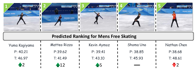
Results on Beijing Winter Olympics

In this part, we show more results of the Beijing 2022 Winter Olympic Games. In the section before, we present the ranking result of ladies short program and pairs free program using our proposed Skating Mixer. To show the advantages of our proposed model, here we choose S-LSTM and MS-LSTM xu2019learning, which have closer performance to our model as shown in the previous section, and apply these two models to the videos in Winter Olympic Games. The result is demonstrated in Figure 1 and 2, respectively. We can see that the predicted ranking results of both models are much worse than those when using our proposed structure. We can also find that S-LSTM generates better results than MS-LSTM which follows the performance shown in the experiment section. This again shows the models can capture some scoring rules and learn to assess figure skating programs. It also demonstrates that our proposed structure is much robust and could extend to other competitions that are not within the training dataset.

Refer to caption — (a) Predicted results on Ladies Short Program

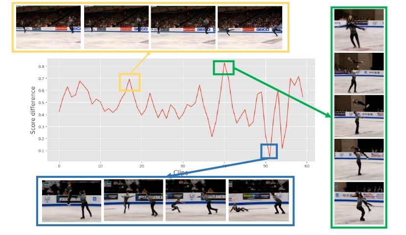
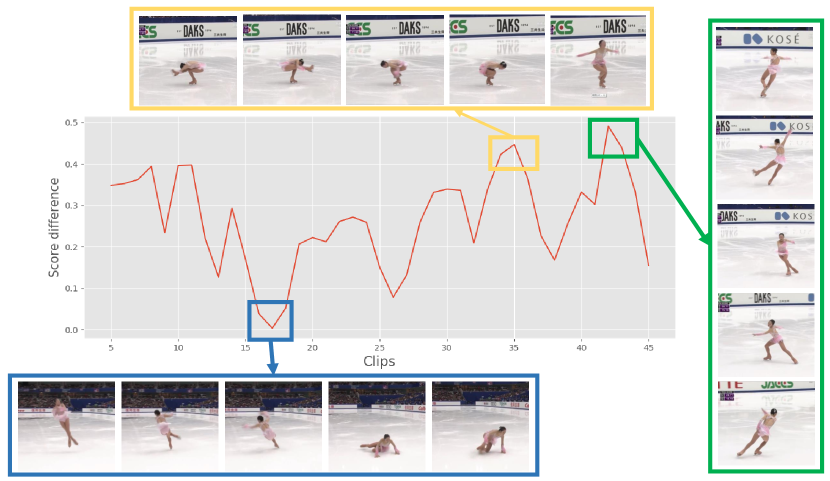
Visualizations

In this part, we show more examples of visualizations as mentioned in the previous section. Figure 3 are two examples from men free program and pairs free program. We can see that when the action is failed, the score for the corresponding clip is relatively low; when the action is successfully done or the move is elegant and fluent, the score is relatively high. In addition, in the pairs free program, the action synchronization is also important for scoring. This implies that our model can learn some basic standards in figure skating scoring.

Core Code

In this section, we show the core code implemented in our structure. Listing 1 demonstrates the code of our proposed memory recurrent unit (MRU). The input memory token is first input to two bottleneck structures to get the information of each modality in previous clips. Then it is concatenated with the feature in the current clip. The features passes through audio mixer, video mixer and multimodal mixer. Finally the output of [CLS] token is mixed with [MEM] in the memory mixer. The [MEM] output is used for the next clip and the [CLS] token outputs are also collected for scoring.

⬇

1def model_forward(self, audio_feature, video_feature, hidden_state=None, back=False):

2

3 if hidden_state is None:

4 hidden_state = self.initial_memory

5

6 prev_audio = self.audio_extraction(hidden_state)

7 prev_video = self.video_extraction(hidden_state)

8

9 if back:

10 concat_audio_input = torch.cat([audio_feature, prev_audio], dim=1)

11 concat_video_input = torch.cat([video_feature, prev_video], dim=1)

12 else:

13 concat_audio_input = torch.cat([prev_audio, audio_feature], dim=1)

14 concat_video_input = torch.cat([prev_video, video_feature], dim=1)

15

16 audio_idx = torch.arange(audio_len + 1)

17 video_idx = torch.arange(video_len + 1)

18

19 audio_pos_encoding = self.audio_pos_embedding(audio_idx)

20 video_pos_encoding = self.video_pos_embedding(video_idx)

21

22 audio_input = concat_audio_input + audio_pos_encoding

23 video_input = concat_video_input + video_pos_encoding

24

25 audio_output = self.audio_mixer(audio_input)

26 video_output = self.video_mixer(video_input)

27

28 cls_token = self.class_token

29

30 multimodal_input = torch.cat([cls_token, audio_output, video_output], dim=1)

31 multimodal_output = self.multimodal_mixer(multimodal_input)

32

33 out_cls = multimodal_output[:, 0:1]

34

35 memory_input = torch.cat([hidden_state, out_cls], dim=1)

36 memory_output = self.memory_mixer(memory_input)

37

38 out_hs = memory_output[:, 0:1]

39

40 return out_hs, out_cls

Listing 1: Code of MRU