Generalized Transport Characterizations for Short Oceanic Internal Waves in a Sea of Long Waves

Abstract

Internal waves in the ocean interact in triads. Early work emphasized the importance of extreme-scale separated interactions in which two large wavenumber waves interact with one small wavenumber wave. More recent efforts have called this early paradigm into question. We use wave turbulence kinetic equation and the ray-tracing WKB technique to derive two versions of the corresponding Fokker-Planck (generalized diffusion) equation. We then use these Fokker-Planck equations to estimate the spectral energy flux towards dissipation (high wave numbers) we obtain different results: spectral transport of the kinetic equation Fokker-Planck equation is an order of magnitude larger than either observations or reported ray tracing estimates. This apparent contradiction stems from the difference between Eulerian and ray-path descriptions of these scale-separated interactions.

1 Introduction

Internal waves are a fascinating phenomenon, ubiquitous in the ocean, and characterized by the oscillation of the invisible surfaces of constant densities of a stratified water column. Internal waves carry a significant fraction of ocean kinetic energy and are an important intermediary in transferring energy and momentum to smaller scales where they are dissipated. There is renewed theoretical interest for investigating the internal waves in the ocean due to recent developments in our ability to perform high-resolution numerical modeling, with internal wave permitting Global Ocean Simulations (Arbic et al., 2018) and regional numerical models (Pan et al., 2020).

The wave turbulence kinetic equation has been used extensively to describe processes of spectral energy transfers between internal waves, see Müller et al. (1986); Polzin and Lvov (2011) for reviews. Early on, special types of resonant three-wave triads characterized by extreme scale separations were identified to play an important role in these spectral energy transfers (McComas and Bretherton, 1977; McComas and Müller, 1981a), yet the details and delicate interbalance of the nonlinear transfers remain an enigma. An important feature of the internal wave kinetic equation is that it diverges for almost all spectral power law indices in the internal wave spectrum (Lvov et al., 2010). This is a mathematical manifestation of the lack of locality in internal wave interactions: nonlinear transfers have significant contributions under extreme scale-separated conditions. The weighting of these extreme scale-separated interactions with spectral power law assumptions results in divergent integrals. Our goal is to understand and to characterize this nonlinear transfer process in this extreme scale-separated limit.

An alternative approach to the wave turbulence kinetic equation is proposed in Henyey et al. (1986), where ray-tracing (or eikonal) techniques are used to describe spectral energy transfers. In this paradigm, the energy cascade is assessed as a net drift $\langle\dot{\bf p}\rangle$ of wave packets toward high wavenumber, where ${\bf p}$ is the momentum of a wave and $\langle\dots\rangle$ represents an ensemble average. Such studies (Henyey et al. (1986); Sun and Kunze (1999b); Ijichi and Hibiya (2017)) provide metrics of the net drift rate at a high wavenumber gate, beyond which waves are considered to ’break’. These numerical simulations are conducted in a ’kitchen sink’ manner in which scale separations in vertical and horizontal wavenumber are viewed as tunable parameters to arrive at downscale transport estimates that align with observations. The alignment requires that the background have similar scales as the wave packet and creates a thematic issue for an asymptotic theory such as ray tracing. A further issue is that a rigorous description of this ensemble average transport $\langle\dot{{\textbf{p}}}\rangle$ is an open question that we address here.

Motivation for our efforts comes from a comparison with the empirical metrics of ocean mixing referred to as ’finescale parameterizations’ Gregg (1989); Polzin et al. (1995), see Polzin et al. (2014) for a review and McComas (1977); McComas and Müller (1981b); Polzin and Lvov (2017); Dematteis et al. (2022) for descriptions of the pivotal role that extreme scale separated interactions play in interpreting the oceanic internal wave spectrum. The most glaring incompatibility of wave turbulence and ray tracing is presented in Section 4: If the mean drift rate in vertical wavenumber is identified as the corresponding gradient of diffusivity as derived from the kinetic equation, then the predicted downscale energy transport is an order of magnitude larger than that supported by the observations. This method parallels assessments for downscale energy transport in ray-tracing numerics (Henyey et al., 1986; Sun and Kunze, 1999b; Ijichi and Hibiya, 2017), but is similarly ten times larger than those numerical results. This disparity has lead us to a systematic examination and physical interpretation of the assumptions within both kinetic equation and ray-path approaches to pinpoint the multiple junctures which might underpin a systematic difference between observation and theory concerning extreme scale separated interactions.

Despite claims by McComas and Bretherton (1977) and Nazarenko et al. (2001) that ray tracing should reduce to the resonant manifold, our understanding is that the kinetic equation and ray tracing differ on fundamental levels. The wave kinetic equation represents the internal wavefield as a system of amplitude modulated waves having constant wavenumber and frequency linked through a dispersion relation. Ray tracing represents a wave-packet as a frequency-modulated system with variations in wavenumber linked to the conservation of an Eulerian phase function. The Fokker-Plank derived in the ray tracing approach additionally represents the average drift of wave packets towards high wave numbers. The role of resonances and off-resonant interactions in the mean drift and dispersion about that mean drift are also different (Polzin and Lvov, 2023), as are the concepts of resonance broadening (Polzin and Lvov, 2017) and bandwidth (Cohen and Lee, 1990) that are important metrics of finite amplitude effects in weakly nonlinear systems.

Our efforts have direct parallels with Kraichnan’s 1959 and 1965 studies (Kraichnan, 1959, 1965) of isotropic homogeneous turbulence using field theoretic techniques. Kraichnan’s 1959 study was an Eulerian based approach which yielded a $k^{-3/2}$ spectrum at high Reynolds number, distinct from Kolmogorov’s $k^{-5/3}$ inertial subrange based upon dimensional analysis. This Eulerian description was labeled the ’Direct Interaction Approximation’ (DIA) and extant data were not sufficient to assess the theoretical prediction. Kraichnan (1965) subsequently understood that the quasi-uniform translation associated with coherent advection at the largest scales (aka sweeping) was creating an artifact wherein the correlation time scale was proportional to the root-mean-square Doppler shift rather than a more intuitive notion that energy transfers between scales depended upon the rate of strain. In 1965 Kraichnan subsequently presented a Lagrangian description (the Abridged Lagrangian History DIA) that isolated the pressure and viscous terms responsible for fluid parcel deformation. The Lagrangian picture resulted in a -5/3 power law and Kolmogorov constant (1.77) quite close to that provided by a summary of atmospheric field data (1.56) (Högström (1996)). The analogy to Kraichnan is that the plane wave formulation corresponds to an Eulerian coordinate system and the Lagrangian coordinate system corresponds to a wave packet formulation in which statistics are accumulated along ray paths.

Similar issues about Doppler shifting arise for internal waves (Holloway, 1980, 1982), Rossby waves (Holloway and Hendershott, 1977; Nazarenko, 2011) and in Magneto-HydroDynamics (Nazarenko et al., 2001). Wave problems are potentially more complicated, in part because the Doppler shifting can be intrinsically related to extreme scale separated interactions, and due to a multiplicity of time scales introduced through resonant interactions absent in 3-D turbulence. In wave turbulence one assumes an expansion in terms of small nonlinearity and an assumption about multiple time scales to assess the evolution of amplitude modulated plane waves. Implicit is a long interaction time scale and a short time scale with regards to the higher orders (Newell, 1968). Reduction of the DIA to the resonant manifold happens as the correlation time scale is small relative to an interaction time scale, and triple correlations associated with nonlinear coupling can be related to the product of two double correlations. Extreme scale separated wave problems can also be treated with ray tracing methods, in which statistics of frequency modulated wave packets are accumulated along ray characteristics rather than Lagrangian trajectories. Ray tracing is an extremely attractive route to deal with sweeping as the dynamics of ray tracing are grounded in the explicit representation of variations in Doppler shifting. It is understood that there are ray method parallels to the interaction and correlation time scales of wave turbulence and the DIA, (McComas and Bretherton, 1977; Nazarenko et al., 2001). However, the time scale definitions for ray methods have not been sufficiently developed for a detailed comparison of the two strategies for assessing the effects of Doppler shifting. In particular, what has been missing is the identification of the interaction time scale. Here we provide a derivation of a generalized transport equation for the evolution of an ensemble of wave packets. This generalized transport equation contains a term representing the ensemble mean drift of wave packets in the spectral domain. This mean drift relates to the interaction time scale and can be directly compared to a correlation time scale relating to dispersion about that mean drift. Having accomplished this, we arrive at the understanding that the resonant bandwidths of weakly nonlinear interactions in the two systems, the DIA kinetic equation and from ray methods, are different; that resonant and non-resonant interactions express themselves differently in the correlation time scale than previously understood; and that spectral transports can be significantly altered by the mean-drift term.

We demonstrate here that it is this simple difference in coordinate systems that leads to the celebrated Garrett and Munk spectrum of the oceanic internal wavefield supporting a net downscale transport. The 3-d action spectrum for the Garrett and Munk spectrum is independent of vertical wavenumber, so that in an Eulerian description there is no vertical wavenumber action gradient to support the diffusion of action regardless of how the vertical component of the diffusivity tensor is defined. In a ray description, the mean drift of wave packets to a high wavenumber can be explicitly represented in an enesmble transport equation and an estimate of the action (energy) available for mixing can be obtained by the counting of wave packets past a sufficiently high wavenumber gate (e.g Henyey et al., 1986).

This paper is organized as follows. Hamiltonian structures and the derivation of transport equations from them are the focal points of Sections 2 and 3. We review the Hamiltonian structure in section 2.1. In Section 2.2 we present a derivation for internal waves that leads to a Fokker-Planck equation. In Section 3 we refine the Hamiltonian structure; extracting only those extreme scale separated interactions in order to derive the Liouville equation (Section 3.1) and its subsequent Fokker-Planck (Section 3.2.4). Subsequent to these theoretical developments we present estimates of energy transport to mixing scales and demonstrate the mismatch between theory and observations in Section 4. We end in Section 5 by discussing this contradiction in light of our derivations. The reader who is primarily interested in the disparity between observations and theory is advised to read section 4 and use the equation references to navigate Sections 2 and 3.

2 Background

2.1 Hamiltonian Structure and Field Variables

The equations of motion satisfied by an incompressible stratified rotating flow in hydrostatic balance are

$$\frac{\partial}{\partial t}\frac{\partial z}{\partial\rho}+\nabla\cdot\left(\frac{\partial z}{\partial\rho}\bf{u}\right) = 0,$$

$$\frac{\partial\bf{u}}{\partial t}+f\bf{u}^{\perp}+\bf{u}\cdot\nabla\bf{u}+\frac{\nabla M}{\rho} = 0,$$

$$\frac{\partial M}{\partial\rho}-gz = 0.$$ (1)

These equations result from mass conservation, horizontal momentum conservation and hydrostatic balance. The equations are written in isopycnal coordinates with the density $\rho$ replacing the height $z$ in its role as an independent vertical variable. Here ${\bf u}=(u,v)$ is the horizontal component of the velocity field, ${\bf u}^{\perp}=(-v,u)$, $\nabla=(\partial/\partial x,\partial/\partial y)$ is the gradient operator along isopycnals, $M$ is the Montgomery potential

$$M=P+g\,\rho\,z\,,$$

with pressure $P$, gravity $g$ and Coriolis parameter $f$.

Here we follow Lvov and Tabak (2004) and take equations (1) and decompose the flow into a potential and a divergence-free part:

$$\bf{u}=\nabla\phi+\nabla^{\perp}\psi\,,$$ (2)

where

$$\nabla^{\perp}=\left(\begin{array}[]{r}-\partial_{y}\\ \partial_{x}\end{array}\right)\,.$$ (3)

The expression for potential vorticity in these coordinates is Haynes and McIntyre (1987)

$${\cal Q}=\frac{f+\partial v/\partial x-\partial u/\partial y}{\Pi},$$ (4)

where $\Pi=\frac{\rho}{g}\partial^{2}M/\partial\rho^{2}=\rho\partial z/\partial\rho$ is a normalized differential layer thickness. Since potential vorticity is conserved along particle trajectories,

$$\frac{D{\cal Q}}{Dt}=0.$$ (5)

The advection of potential vorticity in (5) takes place exclusively along isopycnal surfaces. Therefore, an initial distribution of potential vorticity which is constant on isopycnals, though varying across them, will remain constant. Hence we shall utilize

$${\cal Q}(x,y,\rho,t)=f/\Pi_{0},$$ (6)

where we redefined $\Pi\to\Pi_{0}+\Pi$ to split the potential $\Pi$ into its equilibrium value $\Pi_{0}\equiv-g/N^{2}$ and deviation from it. Stratification $N^{2}$ is permitted to vary with density $\rho$, but is constant along isopycnals. This effectively decouples the internal wavefield from lower frequency flows such as fronts and mesoscale eddies, which are the subject of their own wave turbulence literature (e.g. Müller, 1976; Kafiabad et al., 2019). Such internal wave - mean flow interactions can be a significant regional source of internal wave energy (Polzin, 2010) and may be a key issue in determining the regional character of the internal wavefield (Polzin and Lvov, 2011).

The primitive equations of motion (1) under the assumption (6) can be written as a pair of canonical Hamiltonian equations,

$$\frac{\partial\Pi}{\partial t}=\frac{\delta{\cal H}}{\delta\phi}\,,\qquad\frac{\partial\phi}{\partial t}=-\frac{\delta{\cal H}}{\delta\Pi}\,,$$ (7)

where $\phi$ is the isopycnal velocity potential, and the Hamiltonian is the sum of kinetic and potential energies,

$${\cal H}=\!\!\frac{1}{2}\int\!\!d{\textbf{x}}d\rho\left[\left(\Pi_{0}(\rho)+\Pi({\bf{x}},\rho)\right)\,\left|\nabla\phi({\textbf{x}},\rho)+\frac{f}{\Pi_{0}}\nabla^{{\perp}}\Delta^{-1}\Pi(\bf{x},\rho)\right|^{2}-g\left|\int^{\rho}d\hat{\rho}\frac{\Pi({\textbf{x}},\hat{\rho})}{\hat{\rho}}\right|^{2}\right]$$

(8)

with $\nabla^{\perp}=(-\partial/\partial y,\partial/\partial x)$, $\Delta^{-1}$ is the inverse Laplacian and $\hat{\rho}$ represents a variable of integration.

Our intent is to build a perturbation theory around analytical solutions to the linearized primitive equations as plane waves proportional to $e^{i[{\textbf{r}}\cdot{\textbf{p}}-\sigma t]}$. We therefore transition to the Fourier space:

$$\Pi(x,y,\rho)=\frac{1}{(2\pi)^{3/2}}\int\Pi_{\bf p}\;e^{i{\bf r}\cdot{\bf p}}d{\bf p}, \phi(x,y,\rho)=\frac{1}{(2\pi)^{3/2}}\int\phi_{\bf p}\;e^{i{\bf r}\cdot{\bf p}}d{\bf p},$$

$${\bf p}=({\bf{k}},m), {\bf k}=(k,l), {\bf r}=(x,y,\rho)\;,$$ (9)

and introduce a complex field variable $a_{\bf{p}}$ through the canonical transformation

$$\phi_{\bf{p}}=\frac{iN\sqrt{\sigma_{\bf{p}}}}{\sqrt{2g}|\bf{k}|}\left(a_{\bf{p}}-a^{\ast}_{-{\bf{p}}}\right)\,,\ \ \ \Pi_{\bf{p}}=\frac{\sqrt{g}|\bf{k}|}{\sqrt{2\sigma_{\bf p}}N}\left(a_{\bf{p}}+a^{\ast}_{-{\bf{p}}}\right)\,.$$ (10)

Wave frequency $\sigma_{\bf{p}}$ is restricted to be positive. We ignore variations in density as they multiply horizontal momentum, replacing $\rho$ by a reference density $\rho_{0}$ (the Boussinesq approximation) and arrive at a linear dispersion frequency $\sigma$ given by

$$\sigma_{\bf{p}}=\sqrt{f^{2}+\frac{g^{2}}{\rho_{0}^{2}N^{2}}\frac{|\bf{k}|^{2}}{m^{2}}}\;.$$ (11)

The equations of motion (1) adopt the canonical form

$$i\frac{\partial}{\partial t}a_{\bf{p}}=\frac{\delta{\cal H}}{\delta a_{\bf{p}}^{\ast}}\,,$$ (12)

with Hamiltonian:

$${\cal H}=\int d\bf{p}\,\sigma_{\bf{p}}|a_{\bf{p}}|^{2}$$

$$\quad+\int d{\bf{p}}d{\bf p_{1}}d{\bf p_{2}}\left(\delta_{\bf{p}+\bf{p}_{1}+\bf{p}_{2}}(U_{\bf{p},\bf{p}_{1},\bf{p}_{2}}a_{\bf{p}}^{\ast}a_{\bf{p}_{1}}^{\ast}a_{\bf{p}_{2}}^{\ast}+\mathrm{c.c.})+\delta_{-\bf{p}+\bf{p}_{1}+\bf{p}_{2}}(V_{\bf{p}_{1},\bf{p}_{2}}^{\bf{p}}a_{\bf{p}}^{\ast}a_{\bf{p}_{1}}a_{\bf{p}_{2}}+\mathrm{c.c.})\right).$$

(13)

Here $V_{\bf{p}_{1},\bf{p}_{2}}$ and $U_{\bf{p}_{1},\bf{p}_{2}}$ are the interaction cross sections that define the strength of nonlinear interactions between wave numbers ${\bf p}$, ${\bf p_{1}}$ and ${\bf p_{2}}$ Lvov and Tabak (2001); c.c. denotes the complex conjugate. Implicit in the canonical transformation (10), Hamilton’s equation (12) and Hamiltonian (13) is a time dependence of $e^{-i\sigma t}$. The $U$ elements have a time dependence of $e^{i(\sigma_{{\textbf{p}}_{1}}+\sigma_{{\textbf{p}}_{2}}+\sigma_{{\textbf{p}}_{3}})t}$ with $\sigma_{{\textbf{p}}}>0$. They describe the creation of three waves out of nothing and therefore will not appear in the kinetic equation (LABEL:BroadenedKineticEquation).

This is the standard form of the Hamiltonian of a system dominated by three-wave interactions Zakharov et al. (1992). Calculations of interaction coefficients are tedious but straightforward task, completed in Lvov and Tabak (2004); Lvov et al. (2010). We stress that the field equation (12) with the three-wave Hamiltonian (11, 13) is equivalent to the primitive equations of motion for internal waves (1) with the potential vorticity constraint (6).

2.2 Wave Turbulence theory

In wave turbulence theory, one proposes a perturbation expansion in the amplitude of the nonlinearity, yielding linear waves at the leading order. Wave amplitudes are modulated by the nonlinear interactions, and the modulation is statistically described by a kinetic equation (Zakharov et al., 1992; Nazarenko, 2011) for the wave action spectral density $n_{\bf{p}}$ defined by

$$n_{\bf{p}}\delta(\bf{p}-\bf{p}^{\prime})=\langle a_{\bf{p}}^{\ast}a_{\bf{p}^{\prime}}\rangle.$$ (14)

Here $\langle\dots\rangle$ denotes an ensemble averaging, i.e. averaging over many realizations of the random wave field. Application to the internal wave problem is presented in Section 2b of Lvov et al. (2010).

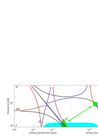
Figure 1: The resonant manifold (2.2.1) in the situation where the three horizontal wavevectors are either parallel or anti-parallel, plotted in a vertical wavenumber - frequency space, for a wave at the center of the green circle. With rotation, extreme scale separations in horizontal wavenumber lead to the extreme scale separated triads mentioned in the introduction. These triads are Bragg scattering (also called elastic scattering, or ES) and a phase velocity equals ground velocity resonance condition, called Induced Diffusion, or (ID) being located at the Coriolis frequency $f$. This study focuses upon the latter class, with scale separation in both horizontal and vertical wavenumber. Near-resonant ID conditions are depicted in green, bandwidth limited non-resonant ID forcing in cyan. The third type of extreme scale separated triads, called Parametric Subharmonic Instability or PSI does not play a role in this manuscript.

2.2.1 Generalized (Broadened) Kinetic Equation:

In the limit of small nonlinearity, one develops a perturbation expansion in the nonlinearity strengh, which leads under certain assumptions to the wave turbulence kinetic equation. The derivation of the resonant kinetic equation is well understood and studied, see Zakharov et al. (1992); Nazarenko (2011). Taking nonresonant interactions leads to a different version of the kinetic equation with the frequency delta functions being replaced by a Lorenzian, see Lvov et al. (1997, 2012). This derivation also hinges on the assessment that fourth order cumulants are a subleading term compared to the product of two double correlators (Deng and Hani, 2021). For the three-wave Hamiltonian (13), the kinetic equation is Eq. (LABEL:BroadenedKineticEquation), describing general internal waves interacting in both rotating and non-rotating environments:

$$\frac{\partial}{\partial t}n_{{\textbf{p}}}=\displaystyle\int\int d{\textbf{p}}_{1}d{\textbf{p}}_{2} \Big{(}\mid V_{{\textbf{p}}_{1},{\textbf{p}}_{2}}^{{\textbf{p}}}\mid^{2}\delta({\textbf{p}}-{\textbf{p}}_{1}-{\textbf{p}}_{2}){\mathcal{L}}(\Delta\sigma_{p12},\Gamma_{p12})[n_{{\textbf{p}}_{1}}n_{{\textbf{p}}_{2}}-n_{{\textbf{p}}}[n_{{\textbf{p}}_{1}}+n_{{\textbf{p}}_{2}}]]$$

$$\left.-\mid V_{{\textbf{p}}_{2},{\textbf{p}}}^{{\textbf{p}}_{1}}\mid^{2}\delta({\textbf{p}}-{\textbf{p}}_{1}+{\textbf{p}}_{2}){\mathcal{L}}(\Delta\sigma_{12p},\Gamma_{p12})[n_{{\textbf{p}}_{2}}n_{{\textbf{p}}}-n_{{\textbf{p}}_{1}}[n_{{\textbf{p}}_{2}}+n_{{\textbf{p}}}]]\right.$$

$$-\mid V_{{\textbf{p}},{\textbf{p}}_{1}}^{{\textbf{p}}_{2}}\mid^{2}\delta({\textbf{p}}+{\textbf{p}}_{1}-{\textbf{p}}_{2}){\mathcal{L}}(\Delta\sigma_{2p1},\Gamma_{p12})[n_{{\textbf{p}}}n_{{\textbf{p}}_{1}}-n_{{\textbf{p}}_{2}}[n_{{\textbf{p}}}+n_{{\textbf{p}}_{1}}]]\Big{)}.$$

where Laurencian $\mathcal{L}$ is given by ${\mathcal{L}}=\frac{\Gamma_{p12}}{(\Delta\sigma)^{2}+\Gamma_{p12}^{2}},$ and $\Delta\sigma_{p12}=\sigma_{p}-\sigma_{p_{1}}-\sigma_{p_{2}}$ represents the distance from the resonant surface. The resonant manifold is defined by

$$\sigma = \sigma_{1}+\sigma_{2};\;\;\;\;\;\;\;\;\;\;\;\bf{p}=\bf{p}_{1}+\bf{p}_{2}$$

$$\sigma = \sigma_{1}-\sigma_{2};\;\;\;\;\;\;\;\;\bf{p}=\bf{p}_{1}-\bf{p}_{2}$$

$$\sigma = \sigma_{2}-\sigma_{1};\;\;\;\;\;\;\bf{p}=\bf{p}_{2}-\bf{p}_{1}\$$ (16)

and appears in figure 1. In wave turbulence theory of internal waves the importance of special extreme scale separated triads was recognized in McComas and Bretherton (1977). These extreme-scale separated limits are called Induced Diffusion (ID), Elastic Scattering (ES) and Parametric Subharmonic Instability (PSI). For an explanation of these triads see, as well, McComas and Müller (1981a).

The total resonance width associated with a specific triad is given by $\Gamma_{p12}=\gamma_{p}+\gamma_{1}+\gamma_{2},$ and the equation for the individual resonance widths is given by

$$\gamma_{p}=\displaystyle\int\int d{\textbf{p}}_{1}d{\textbf{p}}_{2} \Big{(}\mid V_{{\textbf{p}}_{1},{\textbf{p}}_{2}}^{{\textbf{p}}}\mid^{2}\delta({\textbf{p}}-{\textbf{p}}_{1}-{\textbf{p}}_{2}){\mathcal{L}}(\sigma-\sigma_{1}-\sigma_{2})[n_{{\textbf{p}}_{1}}+n_{{\textbf{p}}_{2}}]$$

$$\left.+\mid V_{{\textbf{p}}_{2},{\textbf{p}}}^{{\textbf{p}}_{1}}\mid^{2}\delta({\textbf{p}}-{\textbf{p}}_{1}+{\textbf{p}}_{2}){\mathcal{L}}(\sigma-\sigma_{1}+\sigma_{2})[n_{{\textbf{p}}_{2}}-n_{{\textbf{p}}_{1}}]\right.$$

$$+\mid V_{{\textbf{p}},{\textbf{p}}_{1}}^{{\textbf{p}}_{2}}\mid^{2}\delta({\textbf{p}}+{\textbf{p}}_{1}-{\textbf{p}}_{2}){\mathcal{L}}(\sigma+\sigma_{1}-\sigma_{2})[n_{{\textbf{p}}_{1}}-n_{{\textbf{p}}_{2}}]\Big{)}.$$

Physically this $\gamma_{p}$ represents the fast time scale of decay of a narrow perturbation to the otherwise stationary spectrum (Lvov et al., 1997; Polzin and Lvov, 2017). It coincides with Langevin rates estimated by Pomphrey et al. (1980) and the decay rate of McComas (1977)’s spike experiments. The replacement of the frequency conserving delta function by the Lorentzian takes into account not only resonant, but also near-resonant and nonresonant interactions. Nonresonant interactions appear as a result of the Lorentzian decaying slowly. The role of the nonresonant interactions have to be investigated separately for each particular problem. The detailed investigation that will be presented elsewhere, show that for the case of internal waves and the Garrett and Munk spectrum, the nonresonant interactions leads to the Doppler defect, noticed in Polzin and Lvov (2017).

2.2.2 Fokker-Planck Diffusion Limit

Following McComas and Bretherton (1977) for the resonant kinetic equation, we start from (LABEL:BroadenedKineticEquation) and pick off the interactions having p nearly parallel to ${\textbf{p}}_{1}$ with ${\textbf{p}}_{2}$ small, or nearly parallel to ${\textbf{p}}_{2}$ with ${\textbf{p}}_{1}$ small , which selects the ID class triads. For a sufficiently red spectrum, this permits discarding the small $n_{\textbf{p}}n_{{\textbf{p}}1}$ ($n_{\textbf{p}}n_{{\textbf{p}}2}$, respectively) terms. We then rewrite (LABEL:BroadenedKineticEquation) as

$$\frac{\partial n_{{\textbf{p}}}}{\partial t}=\int d{\textbf{q}}\left({\cal B}({\textbf{p}})-{\cal B}({\textbf{p}}+{\textbf{q}})\right)\simeq-\int d{\textbf{q}}\ \ \left({\textbf{q}}\cdot\frac{\partial}{\partial{\textbf{p}}}\right){\cal B}({\textbf{p}}),$$ (18)

where we introduced

$${\cal B}({\textbf{p}})=8\pi\int|V_{{\textbf{p}}_{1},{\textbf{q}}}^{{\textbf{p}}}|^{2}\,n_{q}(n_{{\textbf{p}}1}-n_{\textbf{p}})\,\delta_{{{\textbf{p}}-{\textbf{p}}_{1}-{\textbf{q}}}}\,{\cal L}({\sigma_{{\textbf{p}}}-\sigma_{{{\textbf{p}}_{1}}}-\sigma_{{{\textbf{q}}}}})d{\textbf{p}}_{1},$$

and expanded the difference $\left({\cal B}({\textbf{p}})-{\cal B}({\textbf{p}}+{\textbf{q}})\right)$ in a Taylor series using q to represent the small difference in wavenumber between the two high frequency waves. Expanding the difference $n_{{\textbf{p}}_{1}}-n_{\textbf{p}}$ for small q gives

$${\cal B}({\textbf{p}})\simeq-8\pi\left({\textbf{q}}\cdot\frac{\partial n_{\textbf{p}}}{\partial{\textbf{p}}}\right)\,\int|V_{{\textbf{p}}_{1},{\textbf{q}}}^{{\textbf{p}}}|^{2}\,n_{q}\delta_{{{\textbf{p}}-{\textbf{p}}_{1}-{\textbf{q}}}}\,{\cal L}({\sigma_{{\textbf{p}}}-\sigma_{{{\textbf{p}}_{1}}}-\sigma_{{{\textbf{q}}}}})d{\textbf{p}}_{1}.$$ (19)

Combining (18) with (19) we obtain

$$\frac{\partial n_{{\textbf{p}}}}{\partial t} = \frac{\partial}{\partial p_{i}}D_{ij}({\textbf{p}},{\textbf{q}})\frac{\partial}{\partial p_{j}}n_{{\textbf{p}}},$$

$$D_{ij}({\textbf{p}},{\textbf{q}}) = 8\pi\int d{\textbf{q}}\left(q_{i}q_{j}\right)|V_{{\textbf{p}}_{1},{\textbf{q}}}^{{\textbf{p}}}|^{2}\,n_{q}\,\delta_{{{\textbf{p}}-{\textbf{p}}_{1}-{\textbf{q}}}}\,{\cal L}({\sigma_{{\textbf{p}}}-\sigma_{{{\textbf{p}}_{1}}}-\sigma_{{{\textbf{q}}}}})d{\textbf{p}}_{1}.$$ (20)

This is a Fokker-Planck diffusion equation describing the diffusion of wave action in the system dominated by nonlocal in wavenumber interactions. Comparison between the Fokker-Planck equation (20) obtained here, and the similar Fokker-Planck equation (obtained using WKB theory (Section 3.2.4 below) will lead to critical insights into the spectral energy transfers in internal wave systems and ultimately to the parametrization of the energy supply to internal wave breaking processes.

3 Wave-Wave interactions in the scale separated limit

In our previous studies Lvov et al. (2010) we have seen that under a scale-invariant assumption, the integrals in the kinetic equation tend to diverge for small or large wave numbers or both. Therefore the interactions via extreme scale separations play an important role in energy exchanges in internal waves. In this section, we are going to develop a rigorous formalism based on WKB techniques to study such interactions.

3.1 The Primitive Equations and Hamiltonian Structure

3.1.1 Reynolds decomposition and Hamiltonian structure

To study interactions between long and short waves we start at (7) and make a Reynolds decomposition in wave amplitude:

$$\Pi\rightarrow\Pi_{0}+\Pi+\pi^{\prime},\ \ \ \ \phi=\Phi+\phi^{\prime},\ \ \ \ \psi=\Psi+\psi^{\prime}\ .$$ (21)

Here the large amplitude waves are represented with $\Pi,\Phi,\Psi$ and small amplitude waves are given by $\phi^{\prime}$, $\pi^{\prime}$ and $\psi^{\prime}$. Given the potentials $\Phi$ and $\phi$, the corresponding velocities are

$${\cal U}=\nabla\Phi+\nabla^{\perp}\Psi,\ \ \ u^{\prime}=\nabla\phi^{\prime}+\nabla^{\perp}\psi^{\prime}.$$

To simplify the presentation we will utilize the non-rotating approximation ($f=0$) in which $(\nabla^{\perp}\Psi,\nabla^{\perp}\psi)\rightarrow 0$. The case of rotating ocean $f\neq 0$ is presented in Appendix.

We substitute the Reynolds decomposition (21) into the equations of motion (1) and subtract equations for the large amplitude waves. The result is given by

$$\dot{\pi}^{\prime}+\nabla\cdot\left((\Pi_{0}+\Pi+\pi^{\prime})\nabla\Phi\right)+\nabla\left(\pi^{\prime}\Phi\right)=0,$$

$$\dot{\phi}^{\prime}+\frac{|\nabla\phi^{\prime}|^{2}}{2}+\nabla\phi^{\prime}\cdot\nabla\Phi+\frac{g}{\rho_{0}^{2}}\int\int d\rho^{\prime}d\rho^{{}^{\prime\prime}}\pi^{\prime}=0.$$

(22)

In these equations $\Pi$ and $\Phi$ are given time-space dependent functions representing the large amplitude waves.

These equations are also Hamilton’s equations,

$$\frac{\partial\pi^{\prime}}{\partial t}=\frac{\delta{\cal H}}{\delta\phi^{\prime}}\,,\qquad\frac{\partial\phi^{\prime}}{\partial t}=-\frac{\delta{\cal H}}{\delta\pi^{\prime}}\,,$$ (23)

with the time-dependent Hamiltonian given by

$${\cal H}=\frac{1}{2}\int d{\bf{r}}\left(\left(\Pi_{0}+\Pi+\pi^{\prime}\right)\,\left|\nabla\phi^{\prime}\right|^{2}+2\pi^{\prime}\nabla\phi^{\prime}\cdot\nabla\Phi-g\left|\int^{\rho}d\hat{\rho}\frac{\pi^{\prime}}{\hat{\rho}}\right|^{2}\right)\,.$$ (24)

There are two types of terms here - those that will ultimately describe a sea of interacting small scale waves and those that will describe the influence of large amplitude large scale waves on the small scale waves. In our previous efforts (Lvov and Tabak, 2001, 2004; Lvov et al., 2010; Polzin and Lvov, 2011, 2017) these terms are comingled. Comparing (8) and (24), we see that (24) contains additional terms $\Pi$$|\nabla\phi^{\prime}|^{2}$ and $\pi^{\prime}\nabla\phi^{\prime}\cdot\nabla\Phi$ that are explicit representations of what will be scale separated interactions. The term $\pi^{\prime}\nabla\phi^{\prime}\cdot\nabla\Phi$ describes the advection of the small-scale internal field by the given large-scale large amplitude field. The term $\Pi$$|\nabla\phi^{\prime}|^{2}$ represents a coupling of small scales to large through changes in the stratification by the large scale wave. The term $\pi^{\prime}|\nabla\phi^{\prime}|^{2}$ will represent interactions local in wavenumber.

We now express the space-dependent variables $\pi^{\prime}({\textbf{r}}),\Pi({\textbf{r}}),\phi^{\prime}({\textbf{r}})$ and $\Phi({\textbf{r}})$ in terms of their Fourier images $\pi^{\prime}({\textbf{p}}),\Pi({\textbf{p}}),\phi^{\prime}({\textbf{p}})$ via (9), make the Boussinesq approximation $\frac{\Pi}{\rho}\simeq\frac{\Pi}{\rho_{0}}$ and use $\int d{\textbf{p}}e^{i{\textbf{p}}\cdot{\textbf{r}}}=(2\pi)^{3}\delta({\textbf{p}})$ to obtain

$${\cal H} = {\cal H}_{\rm linear}+{\cal H}_{\rm nonlinear},$$

$${\cal H}_{\rm linear} = \frac{1}{2}\int d{\textbf{p}}\left(\Pi_{0}|{\bf k}|^{2}|\phi^{\prime}_{{\textbf{p}}}|^{2}-\frac{g}{\rho_{0}^{2}}\frac{|\phi^{\prime}_{{\textbf{p}}}|^{2}}{m^{2}}\right),$$

$${\cal H}_{\rm nonlinear} = {\cal H}_{\rm local}+{\cal H}_{\rm sweeping}+{\cal H}_{\rm density},$$

$${\cal H}_{\rm local} = -{\bf\frac{1}{2(2\pi)^{\frac{3}{2}}}}\int d{\textbf{p}}_{1}d{\textbf{p}}_{2}d{\textbf{p}}_{3}\delta({\textbf{p}}_{1}+{\textbf{p}}_{2}+{\textbf{p}}_{3}){\textbf{k}}_{2}\cdot{\textbf{k}}_{3}\pi^{\prime}_{{\textbf{p}}_{1}}\phi^{\prime}_{{\textbf{p}}_{2}}\phi^{\prime}_{{\textbf{p}}_{3}},$$

$${\cal H}_{\rm sweeping} = -{\bf\frac{1}{2(2\pi)^{\frac{3}{2}}}}\int d{\textbf{p}}_{1}d{\textbf{p}}_{2}d{\textbf{p}}_{3}\delta({\textbf{p}}_{1}+{\textbf{p}}_{2}+{\textbf{p}}_{3})2{\textbf{k}}_{1}\cdot{\textbf{k}}_{2}\Phi_{{\textbf{p}}_{1}}\phi^{\prime}_{{\textbf{p}}_{2}}\pi^{\prime}_{{\textbf{p}}_{3}},$$

$${\cal H}_{\rm density} = -{\bf\frac{1}{2(2\pi)^{\frac{3}{2}}}}\int d{\textbf{p}}_{1}d{\textbf{p}}_{2}d{\textbf{p}}_{3}\delta({\textbf{p}}_{1}+{\textbf{p}}_{2}+{\textbf{p}}_{3}){\textbf{k}}_{2}\cdot{\textbf{k}}_{3}\Pi_{{\textbf{p}}_{1}}\phi^{\prime}_{{\textbf{p}}_{2}}\phi^{\prime}_{{\textbf{p}}_{3}}.$$

The Hamiltonian ${\cal H}_{\rm nonlinear}$ is the sum of three terms:

• ${\cal H}_{\rm local}$ represents small amplitudes interacting with small amplitudes. We will call this term “local” interactions in anticipation of making a scale separation between large amplitude large scale and small amplitude small scale waves in sections 3.1.2 and3.1.3.

• ${\cal H}_{\rm density}$ is the term that describes the variations of stratification that small amplitude waves experience due to the compression and rarification of isopycnals associated with the large amplitude waves. We will refer to this term as a density term.

• ${\cal H}_{\rm sweeping}$ is the term that describes the advection (sweeping) of small amplitude waves by large amplitude waves. In the future, we refer to this term as a sweeping term.

The main focus of this manuscript is to investigate how the density and sweeping terms affect the overall spectral energy density.

3.1.2 Sweeping Hamiltonian

Following the traditional wave turbulence approach, we make a transformation to the wave-action variables that represent wave amplitude and phase:

$$\phi^{\prime}_{\bf p}=\frac{iN\sqrt{\sigma_{\textbf{p}}}}{\sqrt{2g}|{\bf k}|}\left(a_{\textbf{p}}-a^{*}_{-{\textbf{p}}}\right)\,,\ \ \ \pi^{\prime}_{\textbf{p}}=\frac{\sqrt{g}|{\bf k}|}{\sqrt{2\sigma_{\textbf{p}}}N}\left(a_{\textbf{p}}+a^{*}_{-{\textbf{p}}}\right)\,.$$

(27)

We substitute (27) into ${\cal H}_{\rm sweeping}$ of (LABEL:FourierHam), and obtain

$${\cal H}_{\rm sweeping} = -{\bf\frac{1}{2(2\pi)^{\frac{3}{2}}}}\int d{\textbf{p}}_{1}d{\textbf{p}}_{2}d{\textbf{p}}_{3}\delta({\textbf{p}}_{1}+{\textbf{p}}_{2}+{\textbf{p}}_{3})2{\textbf{k}}_{1}\cdot{\textbf{k}}_{2}\Phi_{{\textbf{p}}_{1}}\frac{iN\sqrt{\sigma_{{\textbf{p}}_{2}}}}{\sqrt{2g}|{\bf k}_{2}|}\frac{\sqrt{g}|{\bf k}_{3}|}{\sqrt{2\sigma_{{\textbf{p}}_{3}}}N}$$

$$\hskip 113.81102pt\times\left(a_{{\textbf{p}}_{2}}-a^{*}_{-{\textbf{p}}_{2}}\right)\left(a_{{\textbf{p}}_{3}}+a^{*}_{-{\textbf{p}}_{3}}\right)\,.$$

The next step is algebraically trivial but conceptually fundamental. We invoke an extreme scale separated limit in which the two small amplitude waves have similar frequency and horizontal wavenumber magnitude. No condition is required on the vertical wavenumber. This conditioning retains both the induced diffusion (ID) and Bragg scattering (ES) branches of the resonant manifold, figure 1.

In this scale separated limit of the internal wave problem, $\sigma_{{\textbf{p}}_{2}}\cong\sigma_{{\textbf{p}}_{3}}$ and $|{\bf k}_{2}|\cong|{\bf k}_{3}|$. Beyond the obvious algebraic simplifications, upon expanding the brackets we find terms of the type $a_{{\textbf{p}}_{2}}a_{{\textbf{p}}_{3}}$, $a^{*}_{-{\textbf{p}}_{2}}a^{*}_{-{\textbf{p}}_{3}}$ and $a_{{\textbf{p}}_{2}}a^{*}_{-{\textbf{p}}_{3}}$, $a^{*}_{-{\textbf{p}}_{2}}a_{-{\textbf{p}}_{3}}$. In what follows we neglect the $a_{{\textbf{p}}_{2}}a_{{\textbf{p}}_{3}}$ and $a^{*}_{-{\textbf{p}}_{2}}a^{*}_{-{\textbf{p}}_{3}}$ terms and retain the $a_{{\textbf{p}}_{2}}a^{*}_{-{\textbf{p}}_{3}}$, $a^{*}_{-{\textbf{p}}_{2}}a_{-{\textbf{p}}_{3}}$ terms, since the former terms are nonresonant, while the latter may be in the resonance for some wave numbers. The discarded terms lead to a process when one lower-frequency wave decays into two high-frequency waves and thus the frequencies do not sum to zero. Such decay is a nonresonant process, so we can remove these terms at the onset.

After relabelling subscripts, in which $2\to 1$ and $3\to 2$, we obtain

$${\cal H}_{\rm sweeping} = \int d{\textbf{p}}_{1}d{\textbf{p}}_{2}A_{\rm sweeping}({\textbf{p}}_{1},{\textbf{p}}_{2})a_{{\textbf{p}}_{1}}a^{*}_{{\textbf{p}}_{2}},$$ (29)

$${\rm with}$$

$$A_{\rm sweeping}({\textbf{p}}_{1},{\textbf{p}}_{2}) = -\frac{1}{2}i\left({{\textbf{k}}_{1}-{\textbf{k}}_{2}}\right)\cdot\left({\textbf{k}}_{1}+{\textbf{k}}_{2}\right)\Phi_{{\textbf{p}}_{1}-{\textbf{p}}_{2}}\;.$$

In the limit of large vertical background scales, (3.1.2) describes a quasi-coherent translation of small scale small amplitude waves by the large scale background. At $1/2$ the vertical scale of ${\textbf{p}}_{1}$ and ${\textbf{p}}_{2}$, (3.1.2) describes a Bragg Scattering process. This is distinct from ’local’ interactions as the large amplitude wave has a much larger horizontal scale.

3.1.3 Density Hamiltonian

We now can repeat the same steps for the density Hamiltonian. We substitute (27) into the ${\cal H}_{\rm density}$ of (LABEL:FourierHam), use $\sigma_{{\textbf{p}}_{2}}\cong\sigma_{{\textbf{p}}_{3}}$ and $|{\bf k}_{2}|\cong|{\bf k}_{3}|$, relable subscripts and obtain

$${\cal H}_{\rm density} = \int d{\textbf{p}}_{1}d{\textbf{p}}_{2}A_{\rm density}({\textbf{p}}_{1},{\textbf{p}}_{2})a_{{\textbf{p}}_{1}}a^{*}_{{\textbf{p}}_{2}},$$ (30)

$${\rm with}$$

$$A_{\rm density}({\textbf{p}}_{1},{\textbf{p}}_{2}) = \frac{1}{2\Pi_{0}}\Pi_{{\textbf{p}}_{2}-{\textbf{p}}_{1}}\sqrt{\sigma_{{\textbf{p}}_{1}}\sigma_{{\textbf{p}}_{2}}}\;.$$

In the limit of large vertical background scales, (30) describes the modulation of the background stratification. At $1/2$ the vertical scale of ${\textbf{p}}_{1}$ and ${\textbf{p}}_{2}$, (30) describes a Bragg Scattering process. This is distinct from ’local’ interactions as the large amplitude wave has a much larger horizontal scale.

3.1.4 Quadratic Hamiltonian for inhomogeneous wave turbulence

Let us neglect the local interaction term ${\cal H}_{\rm local}$ in Hamiltonian (LABEL:FourierHam). Then the Hamiltonian (LABEL:FourierHam) of small amplitude small horizontal scale internal waves $a_{\textbf{p}}$ superimposed into a field of large amplitude large horizontal scale internal waves given by space-time-dependent $\Pi$ and $\Phi$ are given by a form that is quadratic in the small-scale variables $a_{{\textbf{p}}}$

$${\cal H} = \int d{\textbf{p}}_{1}d{\textbf{p}}_{2}A({\textbf{p}}_{1},{\textbf{p}}_{2})a_{{\textbf{p}}_{1}}a^{*}_{{\textbf{p}}_{2}},$$ (31)

$${\rm with}$$

$$A({\textbf{p}}_{1},{\textbf{p}}_{2}) = \sigma_{\textbf{p}}\delta({\textbf{p}}_{1}-{\textbf{p}}_{2})+A_{\rm sweeping}({\textbf{p}}_{1},{\textbf{p}}_{2})+A_{\rm density}({\textbf{p}}_{1},{\textbf{p}}_{2}),$$

where $A_{\rm sweeping}({\textbf{p}}_{1},{\textbf{p}}_{2})$ and $A_{\rm density}({\textbf{p}}_{1},{\textbf{p}}_{2})$ are given in (3.1.2) and (30). The $A({\textbf{p}}_{1},{\textbf{p}}_{2})$ are time dependent and depend upon the phases of the external field.

3.2 WKB approach

At this point, we have a three-wave Hamiltonian (3.1.4) with one large-amplitude large horizontal scale wave interacting with two smaller amplitude smaller horizontal scale waves that have similar frequencies. Below we assume a nearly-resonant paradigm and perform algebraic manipulations that take into account the induced diffusion portion of the resonant manifold.

3.2.1 The Wave Packet Transport Equation

In the spatially homogeneous wave turbulence of Section 2.2 we used wave action density $n_{\textbf{p}}$ and a linear dispersion relation $\sigma_{\textbf{p}}$, both being a function of a wave number p. In the case when there is a slowly varying large scale background, i.e. a system where spatial inhomogeneity is present, the properties of wave action and the dispersion relation will depend on the position in space. Then it makes sense to introduce an additional parameter, a position vector r in wave action and linear dispersion relation. The theory for this spatial dependence is developed in Gershgorin et al. (2009) using a Gabor transform to represent the envelope structure describing the spatial localization and carrier frequency. The leading order balance in Gershgorin et al. (2009) leads to action and phase conservation along ray paths. The balance on the envelope scale implies phase modulation, for which we direct the reader to the appendix of Cohen and Lee (1990) for clarity. Associated with the envelope structure is a residual circulation Bühler and McIntyre (2005). The potential for the wave packet to interact with its envelope structure is possible Bühler and McIntyre (2005); Dosser and Sutherland (2011) but would require a modification of the uniform potential vorticity statement (6). It is at this stage that one might also want to consider the potential for nonlinear wave steepening effects associated with ${\cal H}_{\rm local}$ to counter the dispersion of ray characteristics as a precursor to the description of solitary wave dynamics.

The familiar statement of action conservation that we are after is obtained in Gershgorin et al. (2009) by assuming the scale of the envelope structure is large in comparison to the inverse wavenumber of the small scale wave, i.e. the wave packet contains many oscillations. The result required here can be obtained more simply by using a Wigner transform alone to define the space-time dependent wave action spectral density:

$$n_{{\textbf{p}},{\textbf{r}}}\equiv\int e^{i{\textbf{q}}\cdot{\textbf{r}}}\langle a_{{\textbf{p}}+{\textbf{q}}/2}a_{{\textbf{p}}-{\textbf{q}}/2}^{*}\rangle d{\textbf{q}}\;,$$ (32)

in which the transform variable q is a difference between two large wave numbers ${\textbf{p}}_{1}$ and ${\textbf{p}}_{2}$, ${\textbf{q}}={\textbf{p}}_{1}-{\textbf{p}}_{2}$ and the field variables $a$ are evaluated at ${\textbf{p}}\pm{\textbf{q}}/2$. We similarly introduce the space-dependent intrinsic frequency $\omega_{{\textbf{p}},{\textbf{r}}}$

$$\omega_{{\textbf{p}},{\textbf{r}}}=\int e^{i{\textbf{r}}\cdot{\textbf{q}}}A({{\textbf{p}}+{\textbf{q}}/2,{\textbf{p}}-{\textbf{q}}/2})d{\textbf{q}},$$ (33)

This is a generalization of our “traditional” wave action (14) which allows for slow variations of the background. It will incorporate the large vertical scale contributions of ${\cal H}_{{\rm sweeping}}$ and ${\cal H}_{{\rm density}}$.

To derive the transport equation, we take definition (32), differentiate it with respect to time, use Hamilton’s equation of motion (12), with the Hamiltonian (31). The spatial dependence is then made explicit by representing $A({\textbf{p}}_{1},{\textbf{p}}_{2})$ and $a({\textbf{p}}_{1})a^{\ast}({\textbf{p}}_{2})$ with their corresponding Fourier transforms. After an inspired change of variables (Lvov and Rubenchik, 1977; Gershgorin et al., 2009) that maps the ID portion of the resonant manifold, one obtains an intermediary expression:

$$i\frac{\partial n_{{\textbf{p}},{\textbf{r}}}}{\partial t}=\int\frac{d{\textbf{r}}^{\prime}d{\textbf{r}}^{\prime\prime}}{(2\pi)^{6}}dq^{\prime}dq^{\prime\prime}e^{iq^{\prime}\cdot({\textbf{r}}-{\textbf{r}}^{\prime})+iq^{\prime\prime}\cdot({\textbf{r}}-{\textbf{r}}^{\prime\prime})}\mbox{$\left[\rule{0.0pt}{17.07164pt}\right.$}\omega_{{\textbf{p}}+\frac{q^{\prime\prime}}{2}}({\textbf{r}}^{\prime})n_{{\textbf{p}}-\frac{q^{\prime}}{2}}({\textbf{r}}^{\prime\prime})-\omega_{{\textbf{p}}-\frac{q^{\prime\prime}}{2}}({\textbf{r}}^{\prime})n_{{\textbf{p}}+\frac{q^{\prime}}{2}}({\textbf{r}}^{\prime\prime})\mbox{$\left.\rule{0.0pt}{17.07164pt}\right]$}$$ (34)

After expanding $\omega$ and $n$ in Taylor series with respect to p and truncating higher order terms, one ultimately arrive at the action balance:

$$\frac{\partial n_{{\textbf{p}},{\textbf{r}}}}{\partial t}+\nabla_{\textbf{p}}\sigma_{{\textbf{p}},{\textbf{r}}}\cdot\nabla_{{\textbf{r}}}n_{{\textbf{p}},{\textbf{r}}}-\nabla_{\textbf{r}}\sigma_{{\textbf{p}},{\textbf{r}}}\cdot\nabla_{{\textbf{p}}}n_{{\textbf{p}},{\textbf{r}}}=0,$$

(35)

or alternately

$$\frac{\partial n_{{\textbf{p}},{\textbf{r}}}}{\partial t}+\nabla_{{\textbf{r}}}\cdot\mbox{$\left[\rule{0.0pt}{17.07164pt}\right.$}n_{{\textbf{p}},{\textbf{r}}}\nabla_{{\textbf{p}}}\sigma_{{\textbf{p}},{\textbf{r}}}\mbox{$\left.\rule{0.0pt}{17.07164pt}\right]$}-\nabla_{{\textbf{p}}}\cdot\mbox{$\left[\rule{0.0pt}{17.07164pt}\right.$}n_{{\textbf{p}},{\textbf{r}}}\nabla_{{\textbf{r}}}\sigma_{{\textbf{p}},{\textbf{r}}}\mbox{$\left.\rule{0.0pt}{17.07164pt}\right]$}=0.$$

(36)

Integration of (36) over wavenumber provides a connection to the space-time variational formulations found in Witham (1974), Chapters 11.7 and 14. The Bragg scattering process residing in the scale-separated Hamiltonian (3.1.2) has been eliminated by using the Wigner transform and Taylor series expansion that serendipitously exploits the symmetries associated with the ID resonance.

3.2.2 Application for internal waves

We now take the expression for $A_{{\textbf{p}}_{1},{\textbf{p}}_{2}}$ from (31) and substitute it into (33) for the space-dependent linear dispersion relation. The result is given by:

$$\omega_{{\textbf{p}},{\textbf{r}}}=\sigma_{\textbf{p}}-{\textbf{k}}\cdot{\cal U}({\textbf{r}})+\sigma_{\textbf{p}}\frac{\Pi({\textbf{r}})}{2\Pi_{0}},$$ (37)

where ${\textbf{p}}=({\bf k},m)$ is the wavevector, ${\cal U}({\textbf{r}})$ is the time-dependent horizontal velocity of the external large-scale wavefield and $\Pi({\textbf{r}})$ is the time dependent stratification of the external wavefield. Here the $\sigma_{\textbf{p}}$ term was produced by the term proportional to $\delta({\textbf{p}}_{1}-{\textbf{p}}_{2})$, ${\textbf{k}}\cdot{\cal U}$ comes from the sweeping term in the Hamiltonian and $\sigma_{\textbf{p}}\Pi/2\Pi_{0}$ comes from density term in the Hamiltonian. The frequency $\sigma_{\textbf{p}}$ is given by (11) using $f=0$. For a high-frequency wave in a rotating ocean, $\cal{U}$ is replaced by $\nabla\Phi+\nabla^{\perp}\Psi$. The derivation for $f\neq 0$ appears in the Appendix.

3.2.3 The Ray Path Wave Packet Transport Equation

The transport equation (35) or its alternative formulation (36) with the space-time dependent linear dispersion relationship (37) is a fundamental result expressing wave action conservation that provides the basis for the analyses to follow.

The action balance (35) can be simply solved by the method of characteristics. The characteristics of (35), also called rays, are defined by

$$\dot{\textbf{r}}(t) \equiv \nabla_{\textbf{p}}\sigma_{{\textbf{p}},{\textbf{r}}},\ \ \dot{\textbf{p}}(t)\equiv-\nabla_{\textbf{r}}\sigma_{{\textbf{p}},{\textbf{r}}}\;.$$ (38)

Equations (38) imply that wave action spectral density is conserved along these characteristics:

$$\frac{\partial n_{{\textbf{p}},{\textbf{r}}}}{\partial t}+\dot{\textbf{r}}\cdot\nabla_{{\textbf{r}}}n_{{\textbf{p}},{\textbf{r}}}+\dot{\textbf{p}}\cdot\nabla_{{\textbf{p}}}n_{{\textbf{p}},{\textbf{r}}}=0.$$ (39)

This is the classical representation for the conservation of action spectral density along ray trajectories. A derivation for a general Hamiltonian set is presented in Gershgorin et al. (2009), here the derivation is specifically for internal waves in the scale separated limit. Integration over wavenumber provides the space-time result presented in Witham (1974). This result often appears as an analogy to Louiville’s theorem for the conservation of the phase volume of particles without justification. Note that it is the balance of first-order terms in a Taylor series expansion of (34).

3.2.4 An Ensemble Path Transport Equation

In what follows we derive a combined advective-diffusive transport equation for the action balance (35) by generalizing an approach found in Nazarenko et al. (2001). There are strong parallels here to the discussion of Taylor (1921) that appear in the appendix of McComas and Bretherton (1977): The illuminating analogy with particle dispersion in Taylor (1921) is to substitute wavenumber p for the Lagrangian particle position r and obtain a quantitative approach for discussing the migration and dispersion of wave packets in the spectral domain following ray trajectories. Having said this, it should be intuitively obvious that, since particle dispersion in r has little to do with resonance, neither should the issue of dispersion of p in phase space be intrinsically tied to resonance! Yet, an emphasis on the resonant paradigm is the interpretive context pursued in (McComas and Bretherton, 1977; Nazarenko et al., 2001). A second key departure is that our motivation stems from the fact that the GM76 spectrum is a no-flux solution to the Fokker-Planck equation (20). We acknowledge the oceanographic literature in this regard and so are focused upon the issue of a mean drift of wave packets to high wavenumber that is accessible in ray-tracing simulations (e.g. Henyey et al., 1986) but not explicitly represented in (20). To underscore the distinction, the existence of a mean drift implies relative dispersion (e.g. Bennett (1984)) rather than the issue of absolute dispersion addressed in Taylor (1921).

The very first step in our derivation is to specify a wave-packet ensemble mean drift and departures from the mean drift. This decomposition is an improvement on the arguments presented in McComas and Bretherton (1977) and Nazarenko et al. (2001). Our limited knowledge of the ray literature does not permit us from commenting on the originality of our interpretation. It is, however, crucial in understanding intrinsic differences between the kinetic equation and ray theory. Given the nature of our understanding, the issue assuredly carries over to other physical problems such as the interaction of near-inertial waves with lower frequency flows, (e.g. Young and Jelloul, 1997; Kafiabad et al., 2019; Dong et al., 2020) surface gravity wave interaction with lower frequency flows (Villas Boas and Young, 2020) and Rossby wave - Rossby wave interactions Nazarenko (2011).

We represent the wave action of a single wave packet as a sum of a spatially homogeneous part $\overline{n}$ and small “wiggles” $\tilde{n}$:

$$n_{{\textbf{p}},{\textbf{r}}}=\overline{n}_{\textbf{p}}+\tilde{n}_{{\textbf{p}},{\textbf{r}}};\ \ \ n_{\textbf{p}}=\int d{\textbf{r}}\;n_{{\textbf{p}},{\textbf{r}}};\ \ \ \int d{\textbf{r}}\;\tilde{n}_{{\textbf{p}},{\textbf{r}}}=0,$$ (40)

and acknowledge the presence of a mean drift in the spectral domain by adding zero:

$$\dot{{\textbf{p}}}=\dot{{\textbf{p}}}-\langle\dot{{\textbf{p}}}\rangle+\langle\dot{{\textbf{p}}}\rangle\;,$$ (41)

in which $\langle\dots\rangle$ is an ensemble average for a system with spatially homogenous statistics, so that $\langle\dots\rangle$ is independent of r. The mean drift arises due to inhomogeneities of the ray path statistics in the spectral domain. Please note that the dimensions of $\overline{n}_{\textbf{p}}$ and $n_{{\textbf{p}}}$ are different.

Starting from the flux form of the action balance (36), we substitute (40), (41), invoke an ensemble average and integrate over r to obtain

$$\frac{\partial\langle n_{{\textbf{p}}}\rangle}{\partial t}=-\int d{\textbf{r}}\langle\nabla_{\textbf{p}}\cdot[\dot{{\textbf{p}}}-\langle\dot{{\textbf{p}}}\rangle]n_{{\textbf{p}},{\textbf{r}}}\rangle-\nabla_{\textbf{p}}\cdot[\langle\dot{{\textbf{p}}}\rangle\langle n_{{\textbf{p}}}\rangle].$$ (42)

Closure of this equation depends upon writing $n_{{\textbf{p}},{\textbf{r}}}$ in terms of $n_{{\textbf{p}}}$. At this juncture, we invoke that property that wave action spectral density does not change along trajectories:

$$n_{{\textbf{p}},{\textbf{r}}}\equiv n({\textbf{p}}(t),{\textbf{r}}(t),t)=n({\textbf{p}}(t-T),{\textbf{r}}(t-T),t-T)$$

$$=\overline{n}\Big{[}{\textbf{p}}(t)-\int\limits_{t-T}^{t}\dot{p}(t^{\prime})dt^{\prime};\;t-T\Big{]}+\tilde{n}\Big{[}{\textbf{p}}(t)-\int\limits_{t-T}^{t}\dot{p}(t^{\prime})dt^{\prime};\;{\textbf{r}}(t)-\int\limits_{t-\tau}^{t}\dot{\textbf{r}}(t^{\prime})dt^{\prime};\;t-T\Big{]}$$

We then execute a Taylor series expansion of $\overline{n}$,

$$n({\textbf{p}}(t-\tau),{\textbf{r}}(t-\tau),t-\tau)\simeq\overline{n}({\textbf{p}}(t);\;t-T)-\nabla_{p}\overline{n}({\textbf{p}}(t);\;t-T)\cdot\int\limits_{t-T}^{t}\dot{{\textbf{p}}}(t^{\prime})dt^{\prime}+\tilde{n}(\dots)\;,$$

(44)

substitute, add zero once again, and using the definition of ensemble averaging $\langle\dots\rangle$

$$\Big{\langle}\nabla_{{\textbf{p}}}[\dot{{\textbf{p}}}-\big{\langle}\dot{{\textbf{p}}}\big{\rangle}]\overline{n}({\textbf{p}}(t),t-\tau)\Big{\rangle} \cong \nabla_{{\textbf{p}}}\big{\langle}\dot{{\textbf{p}}}-\big{\langle}\dot{{\textbf{p}}}\big{\rangle}\big{\rangle}\big{\langle}\overline{n}({\textbf{p}}(t),t-\tau)\rangle=0$$

and

$$\Big{\langle}\nabla_{{\textbf{p}}}[\dot{{\textbf{p}}}-\big{\langle}\dot{{\textbf{p}}}\big{\rangle}]\int\limits_{t-\tau}^{t}\big{\langle}\dot{{\textbf{p}}}\big{\rangle}dt^{\prime}\cdot\nabla_{{\textbf{p}}}\overline{n}({\textbf{p}}(t),t-\tau)\Big{\rangle} \cong \nabla_{{\textbf{p}}}\big{\langle}\dot{{\textbf{p}}}-\big{\langle}\dot{{\textbf{p}}}\big{\rangle}\big{\rangle}\int\limits_{t-\tau}^{t}\big{\langle}\dot{{\textbf{p}}}\big{\rangle}dt^{\prime}\cdot\nabla_{{\textbf{p}}}\big{\langle}\overline{n}({\textbf{p}}(t),t-\tau)\big{\rangle}$$ (45)

$$= 0$$

as $\langle\dot{{\textbf{p}}}-\langle\dot{{\textbf{p}}}\rangle\rangle\equiv 0$ and neglect an initial transient term

$$\langle\nabla_{{\textbf{p}}}[\dot{{\textbf{p}}}(t)-\langle\dot{{\textbf{p}}}\rangle]\tilde{n}({\textbf{p}}(t-\tau),{\textbf{r}}(t-\tau),t-\tau)\rangle$$ (46)

so that (42) becomes

$$\frac{\partial\langle n_{{\textbf{p}}}\rangle}{\partial t}=-\nabla_{\textbf{p}}\cdot\int\limits_{t-\tau}^{t}\langle[\dot{{\textbf{p}}}(t)-\langle\dot{{\textbf{p}}}\rangle][\dot{{\textbf{p}}}(t^{\prime}-\tau)-\langle\dot{{\textbf{p}}}\rangle]\rangle dt^{\prime}\nabla_{\textbf{p}}\langle n_{{\textbf{p}}}\rangle-\nabla_{\textbf{p}}\langle\dot{{\textbf{p}}}\rangle\langle n_{{\textbf{p}}}\rangle,$$ (47)

We introduce the auto-lag covariance matrix

$${\cal C}_{ij}({\textbf{p}},t,t^{\prime})=\Big{\langle}\Big{[}\dot{\textbf{p}}({\textbf{r}}(t))-\langle\dot{\textbf{p}}({\textbf{r}}(t))\rangle\Big{]}_{i}\Big{[}\dot{\textbf{p}}({\textbf{r}}(t^{\prime}))-\langle\dot{\textbf{p}}({\textbf{r}}(t^{\prime}))\rangle\Big{]}_{j}\Big{\rangle}.$$ (48)

The final result is then

$$\frac{\partial\langle n_{{\textbf{p}}}\rangle}{\partial t}=-\nabla_{{\textbf{p}}_{i}}\cdot\int\limits^{t}_{t-\tau}{\cal C}_{ij}({\textbf{p}},t,t^{\prime})dt^{\prime}\cdot\nabla_{{\textbf{p}}_{j}}\langle n_{\textbf{p}}\rangle\;\;-\;\;\nabla_{{\textbf{p}}_{i}}\langle\dot{\textbf{p}}_{i}\rangle\langle n_{\textbf{p}}\rangle.$$ (49)

Convergence of the time integral, in which one can replace the lower limit of integration by $-\infty$, is the hallmark of a Markov approximation which we investigate further in Polzin and Lvov (2023). This equation encapsulates our fundamental theoretical result: The transport equation changes from diffusion (20) to an expression that involves both advection and diffusion in the spectral domain. Instead of being a no-flux stationary state, the GM76 spectrum, for which $\langle n_{\textbf{p}}\rangle\propto m^{0}$, now supports a downscale action flux.

Our decomposition of wavenumber tendency into mean drift and dispersion about that mean drift provide a concrete mathematical interpretation for an interaction timescale $\tau_{i}$:

$$\tau_{i}^{-1}=|\langle\dot{{\textbf{p}}}\rangle|/|{\textbf{p}}|$$ (50)

and correlation time scale $\tau_{c}$:

$$\tau_{c}=\int\limits^{t}_{-\infty}{\cal C}_{ii}({\textbf{p}},t,t^{\prime})dt^{\prime}/\langle|\dot{\textbf{p}}({\textbf{r}}(t))-\langle\dot{\textbf{p}}({\textbf{r}}(t))|^{2}\rangle\rangle.$$ (51)

Intuitive notions of the interplay between $\tau_{i}$ and $\tau_{c}$ are discussed in Müller et al. (1986) and in Nazarenko et al. (2001) using expressions for ${\cal C}_{ij}$ (48) in which the ensemble mean drift has not been subtracted. The sentiment in Müller et al. (1986) is that a separation between $\tau_{c}$ and $\tau_{i}$ is problematic for the oceanic internal wavefield. Numerical ray tracing results (Henyey and Pomphrey, 1983; Henyey et al., 1984) do not elucidate why this might be. Our decomposition of wavenumber tendency into mean drift and dispersion about that mean drift, the revised Fokker-Planck (49) and revised covariance matrix (48) provide a concrete mathematical interpretation for such judgements about $\tau_{i}$ and $\tau_{c}$.

Having summoned the analogy between particle dispersion Taylor (1921) and dispersion of wavepackets in wavenumber, we are led to a degree of skepticism concerning McComas and Bretherton (1977)’s and Nazarenko et al. (2001)’s interpretation that ray tracing should collapse onto the Fokker-Planck and diffusivity derived from the resonant kinetic equation (20). Convergence of the time-lagged auto-covariance (51) relates a finite diffusivity to the product of a covariance and correlation time scale. If one casts this as a resonant process, the covariance will be infinitely small and the correlation time scale infinitely long, thus leading to an inconsistency between interaction and correlation time scales in the resonant limit. Introducing a broadened kinetic equation (2.2.1) with finite bandwidth helps so much as it changes the ratio of correlation time scale to interaction time scale from infinity to something large, but is not a resolution. As one runs to the finite amplitude of the weakly nonlinear problem, the resonant bandwidth becomes the rms Doppler shift (Polzin and Lvov, 2017). This is aphysical.

We find through numerical experimentation in Polzin and Lvov (2023) that the mean drift $\langle\dot{{\textbf{p}}}\rangle$ is a resonant process and dispersion about the mean drift ${\cal C}_{ij}$ is non-resonant. The latter should not come as a surprise once one appreciates the direct analogy between particle dispersion and ray tracing originally suggested in McComas and Bretherton (1977): particle dispersion in turbulence has nothing to do with the concept of resonance. The moments $\langle\dot{{\textbf{p}}}\rangle$ and ${\cal C}_{ij}$, and changes in the structure and scaling of the resonant bandwidth, are the signature differences of ray theory vs the kinetic equation, paralleling differences between Eulerian (Kraichnan, 1959) and Lagrangian (Kraichnan, 1965) representations of 3-D turbulence. These differences are rooted in the distinctions between amplitude-modulated and frequency-modulated signals.

4 Energy Transport in oceanic internal waves

In Polzin and Lvov (2011, 2017) we note the tension between an apparent pattern match between observed spectral power laws being in apparent agreement with stationary states of the Fokker-Planck equation derived from the kinetic equation (LABEL:BroadenedKineticEquation):

$$\frac{\partial n({\textbf{p}})}{\partial_{m}} + \frac{\partial}{\partial_{m}}D_{33}\frac{\partial}{\partial_{m}}n({\textbf{p}})=0$$ (52)

and this result being inconsistent with what is observationally understood about the energy sources and sinks. Those stationary states come from asserting a balance only in vertical wavenumber, for which there are two families: no-flux states for which $n({\textbf{p}})\propto k^{-x}m^{-y}$ with $y=0$ and constant flux states for which a linear relationship between $x$ and $y$ attains. Both families are oceanographically relevant Polzin and Lvov (2011) and, more to the point, the Garrett and Munk model (GM76) is a member of the no-flux family. This no-flux result attains simply because that spectrum ($(x,y)=(4,0)$) has no gradients in action in vertical wavenumber.

The ray path perspective moves away from this interpretation so that downscale transport is closed as an advective transport (47). Below we explore the downscale energy transport of this advective contribution for the GM76 spectrum, for which

$$D_{33}=\frac{2}{\pi}\frac{km^{2}e_{0}m_{\ast}}{N}\;.$$ (53)

Here $k$ is horizontal wavenumber magnitude, $e_{0}=0.0030$ m² s^-2 is the total energy, $m_{\ast}=4\pi/1300$ m^-1 is a bandwidth parameter, $N=0.0052$ s^-1 is buoyancy frequency and the underlying energy spectrum $e(m,\sigma)$ appears, for example, as equation (5) in Polzin and Lvov (2017). If we associate the mean drift $\langle\dot{m}\rangle$ with $\partial_{m}D_{33}$ derived from the kinetic equation (20) (Polzin and Lvov, 2023) and include a factor of two to account for the two-sided spectral representation, the downscale energy transport is

$$\mathcal{P}=2\int_{f}^{N}\langle\dot{m}\rangle e(m,\sigma)d\sigma=2\big{(}\frac{2}{\pi}\big{)}^{2}\big{(}\frac{e_{0}m_{\ast}}{N}\big{)}^{2}f\log(\frac{N}{f})\cong 1.0\times 10^{-8}[{\rm W\;kg}^{-1}]$$ (54)

which, apart from the prefactor of $1.0\times 10^{-8}$ being an order of magnitude too large, is virtually identical to the finescale parameterization Polzin et al. (2014), their equations 27 and 40. In Polzin and Lvov (2023) we demonstrate through a path integral closure that, indeed, $\langle\dot{m}\rangle=\partial_{m}D$ for the one-dimensional representation of high frequency internal waves interacting with inertial waves. We further demonstrate that both are consistent with simple scale invariant ray-tracing numerical simulations that treat the interaction as a one-dimensional problem. We believe that this one-dimensional treatment is a reasonable representation of extreme scale separated interactions. The one-dimensional version of (20), (52), dates to the dawn of modern oceanography and is supported by basic scale analysis (McComas and Bretherton, 1977; Sun and Kunze, 1999a). It is underpinned by the integrable singularity of the inertial peak in the internal wave frequency spectrum and the lack of horizontal velocity gradients in that peak that is encoded in the dispersion relation. A modern analysis of local and extreme scale separated interactions in a non-rotating context (Dematteis et al., 2022) assigns an energy transport associated with horizontal and diagonal terms of the diffusivity tensor that are an order of magnitude smaller than the Finescale Parameterization, two orders of magnitude smaller than (54). These non-vertical transports are likely overestimates in a rotating paradigm due to the vanishing of horizontal velocity gradients at the inertial peak.

The result (54) stands in dramatic contrast with numerical results concerning the more general problem of high-frequency internal wave packets refracting in a background sea of internal waves (e.g. Henyey et al., 1986; Sun and Kunze, 1999b; Ijichi and Hibiya, 2017). This contention has required a systematic examination and physical interpretation of the assumptions within both kinetic equations (Section 2.2) and ray-path (Section 3.2) approaches to pinpoint the multiple junctures which might underpin a systematic difference between observation and theory concerning extreme scale separated interactions that are presented above in (54).

To date we have identified three potential soft spots that could resolve the contradiction.

The first is that both the ray tracing and kinetic equation discard a coupling between leading order processes that leads to a subtractive cancellation of these leading orders. These leading orders are provided by the induced diffusion mechanism and the Bragg scattering mechanism, in which the phase locking introduced by induced diffusion is damped by Bragg scattering. Both are part of an extreme scale separated Hamiltonian (3.1.2); Bragg scattering is discarded in a Taylor series expansion about the induced diffusion resonance (34) that produces the action conservation statement 35). Representation of this damping process can be defined by bundling eight distinct triads from the resonant manifold; the standard three wave kinetic equation is a perturbation expansion in wave amplitude limited to one triad through a ’random phase’ approximation to obtain (LABEL:BroadenedKineticEquation). This coupling is pursued in the companion manuscript Polzin and Lvov (2023), where we argue that these new physics are the route through which the ocean resolves the contradiction.

The second is that there is the potential for finite amplitude effects in which interactions, both resonant and non-resonant, represent a stochastic forcing in phase space on a short time scale that disrupts the phase-velocity - group velocity resonance on a long time scale. This requires assessment of the resonant bandwidth, which differs in Eulerian (kinetic equation, (LABEL:ResonanceWidth)) versus ray-coordinates, in combination with the amplitude and decorrelation time scales of that forcing. This is investigated more fully in Polzin and Lvov (2023). Our opinion is that (54) and associated scaling is a fundamental metric that should be recoverable by kitchen sink efforts as a small amplitude limit of wave turbulence and using a scale separation that aligns with the assumptions underpinning ray tracing. We offer the opinion that this is how the kitchen sink numerics of ray tracing resolves the contradiction.

The third is that extant efforts at ray tracing high-frequency internal wave packets refracting in a background sea of internal waves (Henyey et al. (1986); Sun and Kunze (1999b); Ijichi and Hibiya (2017)) can not be relied upon as a robust arbiter of this contradiction. Ray tracing is an asymptotic method requiring a scale separation in horizontal wavenumber (3.1.2) in addition to the spatial averaging implied in the envelope structure (3.2.1 Gershgorin et al. (2009)). The ray tracing numerical studies acknowledge none of this and regard scale separation as a tunable parameter. They consistently document sensitivity to the specification of the scale separation and consistently find that the observed finescale metric of energy sourced to turbulent dissipation (Polzin et al. (2014)) requires a scale equivalence, i.e. requires the small parameter of an asymptotic expansion to be $\sim O(1)$. This is the hallmark of interactions represented as ${\cal H}_{\rm local}$ (LABEL:FourierHam) that are spectrally local in wavenumber and need to be treated by other methods Dematteis and Lvov (2021); Dematteis et al. (2022).

5 Conclusions

We have presented two distinct derivations of transport equations for the refraction of high frequency internal waves in inertial wave shear. One derivation results from ’standard’ wave turbulence techniques with the addition of near-resonant interactions and describes the wavefield as a system of amplitude modulated waves. This kinetic equation-based derivation results in a Fokker-Plank equation which returns an estimate of no-net downscale transport in vertical wavenumber for the canonical spectrum of oceanic internal waves referred to as the Garrett-Munk spectrum and small transports associated with horizontal and off-diagonal elements (Dematteis et al., 2022). The second derivation is based on ray-tracing techniques in the WKB limit. Here the ensemble-averaged transport equation (49) contains a mean drift term that is absent from the Fokker Plank equation derived from the kinetic equation (20). This term leads to a prediction of ocean dissipation (54) an order of magnitude greater than supported by ocean observations.

The disparity of these results can be interpreted from an analogy between ray characteristics and Langrangian paths. Recognizing this distinction improves earlier derivations of the ray path transport equation in McComas and Bretherton (1977) and Nazarenko et al. (2001): it provides a rigorous basis for the intuitive characterization of the transport of energy to dissipation invoked in Henyey et al. (1986); Sun and Kunze (1999b); Ijichi and Hibiya (2017). We arrived at this rigorous result by adding zero and explicitly invoking an ensemble average.

Holloway (1980, 1982) argue that internal wave interactions might not be sufficiently weak for wave turbulence theory to be valid. That commentary is directed at inferences the decay rate of narrowband perturbations to the spectrum being much larger than the internal wave frequency Müller et al. (1986). This is inconsistent with the express intent that the kinetic equation describes the slow evolution of the wave spectrum. In Polzin and Lvov (2017) we identify this decay rate is as the small amplitude limit of the resonant bandwidth $\Gamma$ (LABEL:ResonanceWidth). However, the differences in our two Fokker-Planck equations do not hinge upon this issue. We have demonstrated in Polzin and Lvov (2017) that, at finite amplitude, the bandwidth is proportional to the rms Doppler shift. This denotes a degenerate state in which the bandwidth describes the quasi-coherent translation of small-scale waves, i.e. sweeping’, rather than their interaction. In the WKB-based derivation, we operate upon the Hamiltonian with a Wigner transform that integrates over that narrow band perturbation and its nearly resonant decay partners in an extreme scale-separated limit. This removes the apparent discrepancy and arrives at different notions of bandwidth and the role of off-resonant interactions Polzin and Lvov (2017). We investigate these issues in greater detail in Polzin and Lvov (2023).

As we look back over the landscape of this endeavor, what we have is a well-established metric for ocean mixing known as the Finescale Parameterization (Polzin et al., 2014). At best, the Finescale Parameterization is underpinned by a heuristic description as an advective spectral closure (Polzin, 2004a) in the context of an energy transport equation that eschews action conservation in which energy transport in horizontal wavenumber keeps pace with that in vertical wavenumber. This interpretation contrasts with the pivotal role that induced diffusion was perceived to play in determining downscale transports in vertical wavenumber only. A possible resolution can be found in recent characterizations of the internal wave kinetic equation (Dematteis and Lvov, 2021; Dematteis et al., 2022) that coincide in magnitude and scaling with the description of transports encapsulated within the Finescale Parameterization. That work emphasizes the importance of local interactions.

Here we have derived a transport equation (47) based upon a packet ensemble that contains an advective transport term. When the advective transport term is evaluated in a rotating context, it gives rise to a transport estimate (54) that is an order of magnitude greater than the Finescale Parameterization. This inconsistency will be analyzed in Polzin and Lvov (2023), where we suggest that the fourth-order cumulants, which are subleading to the product of two two-point correlators inhomogeneous wave turbulence, are playing a significant role in the spatially inhomogeneous ray-coordinate system.

6 Appendix: Rotations Included

We now repeat all the calculations with rotations included. We start from the primitive equations (1), decompose the velocity using (2), and then use the expression for potential vorticity (4) to obtain:

$$\Pi_{t}+\nabla\cdot\left(\Pi\,\left(\nabla\phi+\nabla^{{\perp}}\Delta^{-1}\left(\frac{f}{\Pi_{0}}\Pi-f\right)\right)\right) = 0\,,$$

$$\phi_{t}+\frac{1}{2}\left|\nabla\phi+\nabla^{{\perp}}\Delta^{-1}\left(\frac{f}{\Pi_{0}}\Pi-f\right)\right|^{2}$$

$$+\Delta^{-1}\nabla\cdot\left[\frac{f}{\Pi_{0}}\Pi\,\left(\nabla^{{\perp}}\phi-\nabla\Delta^{-1}\left(\frac{f}{\Pi_{0}}\Pi-f\right)\right)\right]$$

$$+\frac{g}{\rho}\int^{\rho}\int^{\rho_{2}}\frac{\left(\Pi-\Pi_{0}\right)}{\rho_{1}}\,d\rho_{1}\,d\rho_{2} = 0\,.$$

We now substitute the Reynolds decomposition (21) into (LABEL:PrimitiveEquationHAM). In doing so we use the fact that potential vorticity is assumed to be conserved on isopycnals:

$$\frac{f}{\Pi_{0}}=\frac{f+\Delta\Psi+\Delta\psi^{\prime}}{\Pi_{0}+{\Pi}+\pi^{\prime}}\;.$$

Here we denote by $\Psi+\psi^{\prime}$ the divergence-free part of the velocity field:

$$\Psi+\psi^{\prime}=\Delta^{-1}\left(\frac{f}{\Pi_{0}}(\Pi_{0}+{\Pi}+\pi^{\prime})\right).$$

Then

$$\dot{\pi}^{\prime} + \nabla\cdot\left((\Pi_{0}+\Pi+\pi^{\prime})\left(\nabla\phi^{\prime}+\nabla^{\perp}(\Delta^{-1}(\frac{f\pi^{\prime}}{\Pi_{0}}))\right)\right)+\nabla\cdot\left(\pi^{\prime}\left(\nabla\Phi+\nabla^{\perp}(\Delta^{-1}(\frac{f\Pi)}{\Pi_{0}})\right)\right)=0\,,$$

$$\dot{\phi}^{\prime} + \frac{1}{2}\left|\nabla\phi^{\prime}+\nabla^{\perp}(\Delta^{-1}(\frac{f\pi^{\prime}}{\Pi_{0}})\right|^{2}+\Delta^{-1}\nabla\cdot\left(\frac{f}{\Pi_{0}}(\Pi_{0}+\Pi+\pi^{\prime})(\nabla^{\perp}\phi^{\prime}-\nabla(\Delta^{-1}(\frac{f\pi^{\prime}}{\Pi_{0}}))\right)$$

$$+\Delta^{-1}\cdot\ \nabla\left(\frac{f\pi^{\prime}}{\Pi_{0}}(\nabla^{\perp}\Phi-\nabla(\Delta^{-1}(\frac{f\Pi}{\Pi_{0}})))\right)+\left(\nabla\phi^{\prime}+\nabla^{\perp}(\Delta^{-1}(\frac{f\pi^{\prime}}{\Pi_{0}})\right)\cdot\left(\nabla\Phi+\nabla^{\perp}(\Delta^{-1}(\frac{f\Pi}{\Pi_{0}}))\right)$$

$$\ \ \ \ \ \ \ \ \ +\frac{g}{\rho}\int^{\rho}\int^{\rho_{2}}\frac{\pi^{\prime}}{\rho}\,d\rho_{1}\,d\rho_{2}=0\,.$$

Remarkably, these equations are indeed Hamiltonian, with the Hamiltonian given by

$${\cal H}=\frac{1}{2}\int\Bigg{[}(\Pi_{0}+\Pi+\pi^{\prime})\,\left|\nabla\phi^{\prime}+\nabla^{{\perp}}\Delta^{-1}(\frac{f\pi^{\prime}}{\Pi_{0}})\right|^{2}-g\left|\int^{\rho}\frac{\pi^{\prime}}{\rho_{1}}\,d\rho_{1}\right|^{2}$$

$$+2\pi^{\prime}\left(\nabla\phi^{\prime}+\nabla^{\perp}\Delta^{-1}(\frac{f\pi^{\prime}}{\Pi_{0}})\right)\cdot\left(\nabla\Phi+\nabla^{\perp}\Delta^{-1}(\frac{f\Pi}{\Pi_{0}})\right)\Bigg{]}d{\textbf{r}}\,.$$

(57)

Please compare this with (24).

We now can rewrite the Hamiltonian (57) in the following form:

$${\cal H} = {\cal H}_{\rm linear}+{\cal H}_{\rm nonlinear},$$

$${\cal H}_{\rm linear} = \frac{1}{2}\int\left[\Pi_{0}\left|\nabla\phi^{\prime}+\nabla^{{\perp}}\Delta^{-1}(\frac{f\pi^{\prime}}{\Pi_{0}})\right|^{2}-g\left|\int^{\rho}\frac{\pi^{\prime}}{\rho}\,d\rho_{1}\right|^{2}\right]d{\textbf{r}},$$

$${\cal H}_{\rm nonlinear} = {\cal H}_{\rm local}+{\cal H}_{\rm sweeping}+{\cal H}_{\rm density},$$

$${\cal H}_{\rm local} = \frac{1}{2}\int\pi^{\prime}\left|\nabla\phi^{\prime}+\nabla^{{\perp}}(\Delta^{-1}\frac{f\pi^{\prime}}{\Pi_{0}})\right|^{2}d{\textbf{r}},$$

$${\cal H}_{\rm density} = \frac{1}{2}\int\Pi\left|\nabla\phi^{\prime}+\nabla^{{\perp}}(\Delta^{-1}\frac{f\pi^{\prime}}{\Pi_{0}})\right|^{2}d{\textbf{r}},$$

$${\cal H}_{\rm sweeping} = \int\pi^{\prime}\left(\nabla\phi^{\prime}+\nabla^{\perp}(\Delta^{-1}\frac{f\pi^{\prime}}{\Pi_{0}})\right)\cdot\left(\nabla\Phi+\nabla^{\perp}(\Delta^{-1}\frac{f\Pi}{\Pi_{0}}))\right)d{\textbf{r}}.$$

Making the Fourier transformation and making the Boussinesq approximation allows us to rewrite this in the form that generalizes (LABEL:FourierHam):

$${\cal H} = {\cal H}_{\rm linear}+{\cal H}_{\rm nonlinear},$$

$${\cal H}_{\rm linear} = \frac{1}{2}\int d{\textbf{p}}\left(\Pi_{0}k^{2}|\phi^{\prime}_{{\textbf{p}}}|^{2}+\left(\frac{f^{2}}{k^{2}\Pi_{0}}-\frac{g}{\rho_{0}^{2}m^{2}}\right)|\Pi_{{\textbf{p}}}|^{2}\right)\ ,$$

$${\cal H}_{\rm nonlinear} = {\cal H}_{\rm local}+{\cal H}_{\rm sweeping}+{\cal H}_{\rm density},$$

$${\cal H}_{\rm local} = \frac{1}{2}{\frac{1}{(2\pi)^{3/2}}}\int d{\textbf{p}}_{1}d{\textbf{p}}_{2}d{\textbf{p}}_{3}\delta({\textbf{p}}_{1}+{\textbf{p}}_{2}+{\textbf{p}}_{3})\times\left(-{\textbf{k}}_{2}\cdot{\textbf{k}}_{3}\pi^{\prime}_{{\textbf{p}}_{1}}\phi^{\prime}_{{\textbf{p}}_{2}}\phi^{\prime}_{{\textbf{p}}_{3}}\right.$$

$$\left.\ \ \ \ \ \ \ \ \ \ \ \ \ \ \ \ \ \ \ \ \ \ \ \ \ -(\frac{f}{\Pi_{0}})^{2}\frac{{\textbf{k}}_{2}\cdot{\textbf{k}}_{3}}{k_{2}^{2}k_{3}^{2}}\pi^{\prime}_{{\textbf{p}}_{1}}\pi^{\prime}_{{\textbf{p}}_{2}}\pi^{\prime}_{{\textbf{p}}_{3}}{\bf-}2\frac{f}{\Pi_{0}}\frac{{\textbf{k}}_{2}\cdot{\textbf{k}}_{3}^{{\perp}}}{k_{3}^{2}}\pi^{\prime}_{{\textbf{p}}_{1}}\phi^{\prime}_{{\textbf{p}}_{2}}\pi^{\prime}_{{\textbf{p}}_{3}}\right)\,,$$

$${\cal H}_{\rm density} = \frac{1}{2}{\frac{1}{(2\pi)^{3/2}}}\int d{\textbf{p}}_{1}d{\textbf{p}}_{2}d{\textbf{p}}_{3}\delta({\textbf{p}}_{1}+{\textbf{p}}_{2}+{\textbf{p}}_{3})\left(-{\textbf{k}}_{2}\cdot{\textbf{k}}_{3}\Pi_{{\textbf{p}}_{1}}\phi^{\prime}_{{\textbf{p}}_{2}}\phi^{\prime}_{{\textbf{p}}_{3}}\right.$$

$$\left.\ \ \ \ \ \ \ \ \ \ \ \ \ \ \ \ \ \ \ \ \ -(\frac{f}{\Pi_{0}})^{2}\frac{{\textbf{k}}_{2}\cdot{\textbf{k}}_{3}}{k_{2}^{2}k_{3}^{2}}\Pi_{{\textbf{p}}_{1}}\pi^{\prime}_{{\textbf{p}}_{2}}\pi^{\prime}_{{\textbf{p}}_{3}}{\bf+}2\frac{f}{\Pi_{0}}\frac{{\textbf{k}}_{2}\cdot{\textbf{k}}_{3}^{{\perp}}}{k_{3}^{2}}\Pi_{{\textbf{p}}_{1}}\phi^{\prime}_{{\textbf{p}}_{2}}\pi^{\prime}_{{\textbf{p}}_{3}}\right)\,,$$

$${\cal H}_{\rm sweeping} = {\frac{1}{(2\pi)^{3/2}}}\int d{\textbf{p}}_{1}d{\textbf{p}}_{2}d{\textbf{p}}_{3}\delta({\textbf{p}}_{1}+{\textbf{p}}_{2}+{\textbf{p}}_{3})\times\left(-{\textbf{k}}_{2}\cdot{\textbf{k}}_{3}\pi^{\prime}_{{\textbf{p}}_{1}}\phi^{\prime}_{{\textbf{p}}_{2}}\Phi_{{\textbf{p}}_{3}}\right.$$

$$\left.\hskip-56.9055pt{\bf+}\frac{f}{\Pi_{0}}\frac{{\textbf{k}}_{2}\cdot{\textbf{k}}_{3}^{\perp}}{k_{3}^{2}}\pi^{\prime}_{{\textbf{p}}_{1}}\phi^{\prime}_{{\textbf{p}}_{2}}\Pi_{{\textbf{p}}_{3}}{\bf+}\frac{f}{\Pi_{0}}\frac{{\textbf{k}}_{2}^{\perp}\cdot{\textbf{k}}_{3}}{k_{2}^{2}}\pi_{{\textbf{p}}_{1}}^{\prime}\pi^{\prime}_{{\textbf{p}}_{2}}\Phi_{{\textbf{p}}_{3}}{\bf-}(\frac{f}{\Pi_{0}})^{2}\frac{{\textbf{k}}_{2}\cdot{\textbf{k}}_{3}}{k_{2}^{2}k_{3}^{2}}\pi^{\prime}_{{\textbf{p}}_{1}}\pi^{\prime}_{{\textbf{p}}_{2}}\Pi_{{\textbf{p}}_{3}}\right)\,,$$

The next step is to substitute formulas for $\Pi_{\textbf{q}}$ and $\Phi_{\textbf{q}}$ from (10), and to perform the steps and approximations that are developed in sections (3.1,3.2). Results are the generalization of the (3.1.4), and (3.1.2) and (30):

$${\cal H} = \int d{\textbf{p}}_{1}d{\textbf{p}}_{2}A^{f}({\textbf{p}}_{1},{\textbf{p}}_{2})a_{{\textbf{p}}_{1}}a^{*}_{{\textbf{p}}_{2}},$$

$${\rm with}$$

$$A^{f}({\textbf{p}}_{1},{\textbf{p}}_{2}) = \omega_{{\textbf{p}}_{1}}\delta({\textbf{p}}_{1}-{\textbf{p}}_{2})+A_{\rm sweeping}({\textbf{p}}_{1},{\textbf{p}}_{2})+A_{\rm density}^{f}({\textbf{p}}_{1},{\textbf{p}}_{2}),$$

$$A_{\rm sweeping}^{f}({\textbf{p}}_{1},{\textbf{p}}_{2}) = \frac{1}{(2\pi)^{3/2}}\left(\frac{1}{2}i\left({{\textbf{k}}_{1}-{\textbf{k}}_{2}}\right)\cdot\left({\textbf{k}}_{1}+{\textbf{k}}_{2}\right){\bf+}\frac{f}{\Pi_{0}}{\textbf{k}}_{1}\cdot{\textbf{k}}_{2}^{\perp}(\frac{1}{k_{2}^{2}}{\bf-}\frac{1}{k_{1}^{2}})\frac{gk_{1}k_{2}}{2\sqrt{\omega_{1}\omega_{2}}N^{2}}\right)\Phi_{{\textbf{p}}_{2}-{\textbf{p}}_{1}}$$

$$+ \left(\frac{{\bf-}i\frac{f}{\Pi_{0}}{\textbf{k}}_{1}^{\perp}\cdot{\textbf{k}}_{2}}{|{\textbf{k}}_{2}-{\textbf{k}}_{1}|^{2}}-(\frac{f}{\Pi_{0}})^{2}\frac{({\textbf{k}}_{2}-{\textbf{k}}_{1})}{({{\textbf{k}}_{1}-{\textbf{k}}_{2}})^{2}}\cdot(\frac{{\textbf{k}}_{2}}{k_{2}^{2}}+\frac{{\textbf{k}}_{1}}{k_{1}^{2}})\frac{gk_{1}k_{2}}{2\sqrt{\omega_{1}\omega_{2}}N^{2}}\right)\Pi_{{\textbf{p}}_{2}-{\textbf{p}}_{1}},$$

$$A_{\rm density}^{f}({\textbf{p}}_{1},{\textbf{p}}_{2}) = \frac{1}{(2\pi)^{3/2}}\left(\frac{N^{2}}{2g}\sqrt{\omega_{{\textbf{p}}_{1}}\omega_{{\textbf{p}}_{2}}}\frac{{\textbf{k}}_{2}\cdot{\textbf{k}}_{3}}{k_{2}k_{3}}+\frac{i}{2}\frac{g}{N^{2}}\frac{f^{2}}{\Pi_{0}^{2}\sqrt{\omega_{{\textbf{p}}_{1}}\omega_{{\textbf{p}}_{2}}}}\right)\Pi_{{\textbf{p}}_{1}-{\textbf{p}}_{2}}.$$

Using these equations and repeating steps above and discarding terms proportional to $q^{2}$ leads to

$$\omega({\textbf{p}},{\textbf{r}}) = \sigma_{\textbf{p}}-{\textbf{k}}\cdot\nabla\Phi({\textbf{r}},t)-\frac{f}{\Pi_{0}}{\textbf{k}}\cdot\nabla^{\perp}\Delta^{-1}\Pi({\textbf{r}},t)$$

$$+\frac{N^{2}}{2g}\Pi({\textbf{r}},t)\sigma_{\bf p}$$

$$+ \frac{f^{2}g}{\Pi_{0}^{2}\omega_{p}N^{2}}\Pi({\textbf{r}},t)+\frac{f^{2}g}{2\omega_{\textbf{p}}\Pi_{0}^{2}N^{2}}\int\cos({2\theta_{{\textbf{q}}{\textbf{p}}}})\Pi({\textbf{q}},t)e^{i{\textbf{r}}\cdot{\textbf{q}}}dq.$$

Here $\theta_{{\textbf{q}}{\textbf{p}}}$ is an angle between the horizontal part of wave vector ${\bf q}={\textbf{p}}_{1}-{\textbf{p}}_{2}$ (32) and the horizontal part of ${\bf p}$, that is ${\bf k}$, with the sign defined using the right-hand rule going from $q$ TO $p$. The Eulerian frequency $\sigma_{\textbf{p}}$ is given by (11). Note that the first line is simply $\sigma_{\textbf{p}}-{\textbf{k}}\cdot{\cal U}$, the second line is the density term that we have considered above, and the third line is the contribution from a rotating ocean. Equation (37), which is lines one and two of (LABEL:FinalEquationTookMeTwoMonthsToDerive) with $\cal{U}$$=\nabla\Phi$, applies to a non-rotating ocean. In a rotating ocean, a wave whose frequency is high enough not to be impacted by rotation is described using lines one and two.

References

- (1)
- Arbic et al. (2018) Arbic, B. K., M. Alford, J. Ansong, M. C. Buijsman, R. B. Ciotti, J. T. Farrar, R. W. Hallberg, C. E. Henze, C. N. Hill, C. A. Luecke and others (2018), A primer on global internal tide and internal gravity wave continuum modeling in HYCOM and MITgcm. New frontiers in operational oceanography.
- Bennett (1984) Bennett, AF (1984), Relative dispersion: Local and nonlocal dynamics. J. Atmos. Sci., 41, 881–1886.
- Bühler and McIntyre (2005) Bühler, O. and M. E. McIntyre (2005), Wave capture and wave-vortex duality. J. Fluid Mech., 534, 67–95.
- Cohen and Lee (1990) Cohen, L.; Lee C. Instantaneous bandwidth for signals and spectrogram. Proc. IEEE Int. Conf. Acoust. Speech Signal Processing , 1990 2451–2454.
- Dematteis and Lvov (2021) Dematteis, G., and Y. Lvov (2021), Downscale energy fluxes in scale invariant oceanic internal wave turbulence, J. Fluid Mech., 915 , A129 (2021).
- Dematteis et al. (2022) Dematteis, G. K.L. Polzin and Y. V. Lvov, (2022), On the Origins of the Oceanic Ultraviolet Catastrophe, J. Phys. Oceanogr., accepted.
- Dematteis and Lvov (2023) Dematteis,G. and Yuri V Lvov, (2023), Structure of Energy Fluxes in Wave Turbulence, J. of Fluid Mechanics, 954, A30, doi:10.1017/jfm.2022.995
- Deng and Hani (2021) Deng, Y. and Z. Hani (2021), Full Derivation of the Kinetic Equation. arXiv:2104.11204v3math.AP]5Jul2021
- Dong et al. (2020) Dong, W., O. Bühler and K. S. Smith (2020), Frequency diffusion of waves by unsteady flows. J. Fluid Mech., 905.
- Dosser and Sutherland (2011) Dosser, H. and Sutherland, B. (2011), Anelastic internal wave packet evolution and stability. J. Atmos. Sci., 68, 2844–2859.
- Nazarenko et al. (2001) Nazarenko, S. V. and and A. C. Newell and S. V. Galtier, (2001): Nonlocal MHD turbulence. Physica D, 152-153. 646-652.
- Garrett and Munk (1972) Garrett, C. J. R. and W. H. Munk (1972), Space-time scales of internal waves. Geophysical Fluid Dynamics, 3, 225–264.
- Garrett and Munk (1979) Garrett, C. J. R. and W. H. Munk (1979), Internal waves in the ocean. Ann. Rev. Fluid Mech., 11, 339–369.
- Gershgorin et al. (2009) Gershgorin, B., Y. V. Lvov and S. Nazarenko (2009), Canonical Hamiltonians for waves in inhomogeneous media. J. of Math. Physics, .
- Gregg (1989) Gregg, M. C. (1989), Scaling turbulent dissipation in the thermocline. J. Geophys. Res., 94, 9686–9698.
- Haynes and McIntyre (1987) Haynes, Peter H and McIntyre, Michael E, 1987: On the evolution of vorticity and potential vorticity in the presence of diabatic heating and frictional or other forces, J. Atmos. Sci., 44, 828–841.
- Henyey et al. (1986) Henyey, F. S., J. Wright, and S. M. Flatté (1986), Energy and action flow through the internal wave field. An eikonal approach. J. Geophys. Res., 91, 8487–8495.
- Henyey and Pomphrey (1983) Henyey, F. S., and N. Pomphrey (1983), Eikonal description of internal wave interactions: A non-diffusive picture of ”induced diffusion”. Dyn. Atmos. Oceans, 7, 189–208.
- Henyey et al. (1984) Henyey, F. S., N. Pomphrey, and J. D. Meiss (1984), Comparison of short-wavelength internal wave transport theories. LJI-R-84-248, La Jolla Institute.
- Högström (1996) Högström, U.L.F. (1996), Review of some basic characteristics of the atmospheric surface layer. Boundary-Layer Meteorology, 78, 215–246.
- Holloway (1980) Holloway, G. (1980), Oceanic internal waves are not weak waves. J. Phys. Oceanogr., 10, 906–914.
- Holloway (1982) Holloway, G. (1982), On interaction timescales of oceanic internal waves. J. Phys. Oceanogr., 12, 293–296.
- Holloway and Hendershott (1977) Holloway, G. and M.C. Hendershott (1977), Stochastic closure for nonlinear Rossby waves. J. Fluid Mech., 82, 747–765.
- Ijichi and Hibiya (2017) Ijichi, T. and T. Hibiya (2017), Eikonal calculations for energy transfer in the deep-ocean internal wave field near mixing hotspots. J. Phys. Oceanogr., 47, 199-210.
- Kafiabad et al. (2019) Kafiabad, H. A., A. Savva, A. C. Miles and J. Vanneste (2019), Diffusion of inertia-gravity waves by geostrophic turbulence. J. Fluid Mech., 869.
- Kraichnan (1959) Kraichnan, R.H. (1959), The structure of isotropic turbulence at very high Reynolds numbers. J. Fluid Mech., 5, 497–543.
- Kraichnan (1965) Kraichnan, R.H. (1965), Lagrangian-history closure approximation for turbulence. The Physics of Fluids, 8, 575–598.
- Lvov et al. (1997) Lvov, V. S., Lvov, Y. V., Newell, A. C. and Zakharov,V. E. (1997), Statistical description of acoustic turbulence, Phys. Rev. E, 56, 390–405.
- Lvov and Tabak (2001) Lvov, Y. V., and E. G. Tabak (2001): Hamiltonian formalism and the Garrett and Munk spectrum of internal waves in the ocean. Phys. Rev. Lett., 87, 169501-1–168501-4.
- Lvov et al. (2004) Lvov, Y. V., K. L Polzin and E. Tabak (2004), Energy spectra of the ocean’s internal wave field: theory and observations Physical Review Letters, 92, 128501.
- Lvov and Tabak (2004) Lvov, Y.V., and Tabak E.G. (2004), A Hamiltonian Formulation for Long Internal Waves. Physica D, 195 106-122.
- Lvov et al. (2010) Lvov, Y.V., K. L. Polzin, E. G. Tabak, and N. Yokoyama (2010), Oceanic internal wavefield: Theory of scale-invariant spectra, J. Physical Oceanogr., 40, 2605–2623.
- Lvov et al. (2012) Lvov, Y.V., K. L. Polzin and N. Yokoyama (2012), Resonant and near-resonant internal wave interractions, J. Phyisical Oceanogr., 42, 669–691.
- Lvov and Rubenchik (1977) Lvov, V.S. and Rubenchik (1977), Sov. Phys. JETP, 45, 67. Also at V.S. Lvov, Fundamentals of Nonlinear Physics, Lecture Notes, Eq.s 7.7-7.8, www.lvov.weizmann.ac.il.
- McComas (1977) McComas, C. H. (1977), Equilibrium mechanisms within the oceanic internal wavefield, J. Phys. Oceanogr., 7, 836–845.
- McComas and Bretherton (1977) McComas, C. H., and F. P. Bretherton (1977), Resonant interaction of oceanic internal waves. J. Geophys. Res., 83, 1397–1412.
- McComas and Müller (1981a) McComas, C. H., and P. Müller (1981a): Timescales of resonant interactions among oceanic internal waves. J. Phys. Oceanogr., 11, 139–147.
- McComas and Müller (1981b) McComas, C. H., and P. Müller (1981b): The dynamic balance of internal waves. J. Phys. Oceanogr., 11, 970–986.
- Marshall et al. (2012) Marshall, D. P., J. R. Maddison and P. S. Berloff (2012), A framework for parameterizing eddy potential vorticity fluxes. J. Phys. Oceanogr., 42, 539–557.
- Müller (1976) Müller, P. (1976), On the diffusion of momentum and mass by internal gravity waves. J. Fluid Mech., 77, 789–823.
- Müller et al. (1986) Müller, P., G. Holloway, F. Henyey, and N. Pomphrey (1986), Nonlinear interactions among internal gravity waves. Rev. Geophys., 24, 493–536.
- Nazarenko (2011) Nazarenko, S. (2011), Wave Turbulence. Springer Science & Business Media.
- Newell (1968) Newell, A. C. (1968), The closure problem in a system of random gravity waves. Rev. Geophys., 6, 1–31.
- Pan et al. (2020) Pan, Y., B. K. Arbic, A. D. Nelson, D. Menemenlis, W. R. Peltier, W. Xu and Y. Li, (2020), Numerical investigation of mechanisms underlying oceanic internal gravity wave power-law spectra. J. Phys. Oceanogr., 50, 2713-2733.
- Peierls (1929) Peierls, R. (1929), Zur kinetshen Theorie der Warmeleitungen in Kristallen,Ann. Phys., 3, 1055-1101.
- Polzin (2004a) Polzin, K. L. (2004) A heuristic description ofinternal wave dynamics. J. Phys. Oceanogr., 34(1), 214–230.
- Polzin et al. (1995) Polzin, K. L., J. M. Toole and R. W. Schmitt (1995), Finescale parameterizations of turbulent dissipation, J. Phys. Ocean., 25, 306–328.
- Polzin (2010) Polzin, K. L. (2010) Mesoscale-Eddy Internal Wave Coupling. II. Energetics and Results from PolyMode. J. Phys. Oceanogr., 40, 789–801.
- Polzin and Lvov (2011) Polzin, K. L., and Y. S. Lvov (2011) Toward regional characterizations of the oceanic internal wave spectrum. Rev. Geophys., Rev. Geophys., 49, doi:10.1029/2010RG000329.
- Polzin et al. (2014) Polzin, K. L., A. C. Naveira Garabato, B. M. Sloyan, T. Huussen and S. N. Waterman Finescale Parameterizations of Turbulent Dissipation. J. Geophys. Res, 119, 1383?1419
- Polzin and Lvov (2017) Polzin, K. L., and Y. S. Lvov (2017) An Oceanic Ultra-Violet Catastrophe, Wave-Particle Duality and a Strongly Nonlinear Concept for Geophysical Turbulence. Fluids, 2, 36; doi:10.3390/fluids2030036.
- Polzin and Lvov (2023) Polzin, K. and Y. Lvov, Scale Separated Interactions of Oceanic Internal Waves: A One-Dimensional Model in preparation
- Pomphrey (1981) Pomphrey, N.(1981), Review of some calculations of energy transport in a Garrett-Munk ocean, in Nonlinear Properties of Internal Waves, edited by B. J. West, 114-128, American Institute of Physics, New York, 1981.
- Pomphrey et al. (1980) Pomphrey, N., J. D. Meiss and K. M. Watson (1980), Description of nonlinear internal wave interactions using Langevin methods. J. Geophys. Res., 85, 1085–1094.
- Savva et al. (2021) Savva, M. and Kafiabad, H. A. and Vanneste, J. (2021): Inertia-gravity-wave scattering by three-dimensional geostrophic turbulence. J. Fluid Mech., 916.
- Sun and Kunze (1999a) Sun, H., and E. Kunze (1999), Internal wave–wave interactions. Part I: The role of internal wave vertical divergence. J. Phys. Oceanogr., 29, 2886–2904.
- Sun and Kunze (1999b) Sun, H., and E. Kunze (1999), Internal wave–wave interactions. Part II: Spectral energy transfer and turbulence production. J. Phys. Oceanogr., 29, 2905–2919.
- Taylor (1921) Taylor, G. I. (1921) Diffusion by continuous movements.
- Villas Boas and Young (2020) Villas Bôas, A. B. and W. R. Young (2020), Directional diffusion of surface gravity wave action by ocean macroturbulence. J. Fluid Mech., 890.
- Vlasov (1961) Vlasov, A. A. (1961). Many-Particle Theory and Its Application to Plasma. New York.
- Witham (1974) Witham, G. B., (1974), Linear and Nonlinear Waves. Wiley-Interscience, New York, pp. 636.
- Young and Jelloul (1997) Young, W. R. and M. B. Jelloul (1997), Propagation of near-inertial oscillations through a geostrophic flow. J. of marine research, 55, 735–766.
- Zakharov et al. (1992) Zakharov, V. E., V. S. Lvov, and G. Falkovich (1992), Kolmogorov Spectra of Turbulence. Springer-Verlag.