ALMA-IMF III - Investigating the origin of stellar masses: Top-heavy core mass function in the W43-MM2&MM3 mini-starburst

Abstract

Aims. The processes that determine the stellar initial mass function (IMF) and its origin are critical unsolved problems, with profound implications for many areas of astrophysics. The W43-MM2&MM3 mini-starburst ridge hosts a rich young protocluster, from which it is possible to test the current paradigm on the IMF origin.

Methods. The ALMA-IMF Large Program observed the W43-MM2&MM3 ridge, whose 1.3 mm and 3 mm ALMA 12 m array continuum images reach a $\sim$2 500 au spatial resolution. We used both the best-sensitivity and the line-free ALMA-IMF images, reduced the noise with the multi-resolution segmentation technique MnGSeg, and derived the most complete and most robust core catalog possible. Using two different extraction software packages, getsf and GExt2D, we identified $\sim$200 compact sources, whose $\sim$100 common sources have, on average, fluxes consistent to within 30%. We filtered sources with non-negligible free-free contamination and corrected fluxes from line contamination, resulting in a W43-MM2&MM3 catalog of 205 getsf cores. With a median deconvolved FWHM size of 3 400 au, core masses range from $\sim$0.1$\leavevmode\nobreak\ M_{\odot}$ to $\sim$70$\leavevmode\nobreak\ M_{\odot}$ and the getsf catalog is 90% complete down to $0.8\leavevmode\nobreak\ M_{\odot}$.

Results. The high-mass end of the core mass function (CMF) of W43-MM2&MM3 is top-heavy compared to the canonical IMF. Fitting the cumulative CMF with a single power-law of the form $N(>\log M)\propto M^{\rm\alpha}$, we measured $\alpha=-0.95\pm 0.04$, compared to the canonical $\alpha=-1.35$ Salpeter IMF slope. The slope of the CMF is robust with respect to map processing, extraction software packages, and reasonable variations in the assumptions taken to estimate core masses. We explore several assumptions on how cores transfer their mass to stars (assuming a mass conversion efficiency) and subfragment (defining a core fragment mass function) to predict the IMF resulting from the W43-MM2&MM3 CMF. While core mass growth should flatten the high-mass end of the resulting IMF, core fragmentation could steepen it.

Conclusions. In stark contrast to the commonly accepted paradigm, our result argues against the universality of the CMF shape. More robust functions of the star formation efficiency and core subfragmentation are required to better predict the resulting IMF, here suggested to remain top-heavy at the end of the star formation phase. If confirmed, the IMFs emerging from starburst events could inherit their top-heavy shape from their parental CMFs, challenging the IMF universality.

1 Introduction

The stellar initial mass function (IMF), which characterizes the mass distribution of stars between $0.01\leavevmode\nobreak\ M_{\odot}$ and $>100\leavevmode\nobreak\ M_{\odot}$, has long been considered universal (see, e.g., reviews by Bastian et al. 2010; Kroupa et al. 2013). The IMF, which is therefore qualified as canonical, is often represented by a lognormal function peaking at stellar masses around $0.2-0.3\leavevmode\nobreak\ M_{\odot}$, connected to a power-law tail, $\frac{{\rm d}N}{{\rm d}\log M}\propto M^{-1.35}$, that dominates for masses larger than $1\leavevmode\nobreak\ M_{\odot}$ (Chabrier 2005). Following the functional description of the IMF by Salpeter (1955) and Scalo (1986), Kroupa et al. (1993) proposed another representation based on a series of three broken power-laws. In this representation, which was later refined by Kroupa (2002), the form of the IMF would follow $\frac{{\rm d}N}{{\rm d}\log M}\propto M^{0.7}$ in the range $0.01-0.08\leavevmode\nobreak\ M_{\odot}$, $\frac{{\rm d}N}{{\rm d}\log M}\propto M^{-0.3}$ in the range $0.08-0.5\leavevmode\nobreak\ M_{\odot}$, and $\frac{{\rm d}N}{{\rm d}\log M}\propto M^{-1.3}$ for $M>0.5\leavevmode\nobreak\ M_{\odot}$. The power-laws at the high-mass end of these two representations correspond, within the limits of observational uncertainties, to the description of Salpeter (1955), $\frac{{\rm d}N}{{\rm d}\log M}\propto M^{-1.35}$, which becomes $N(>\log M)\propto M^{-1.35}$ in its complementary cumulative distribution form. The IMF universality, which has been postulated on the basis of studies of field stars and young stellar clusters in the solar vicinity (up to a few hundred of parsecs), has recently been challenged in more extreme environments. Observations of young massive clusters in the Milky Way (Lu et al. 2013; Maia et al. 2016; Hosek et al. 2019), in nearby galaxies (Schneider et al. 2018), and of high-redshift galaxies (Smith 2014; Zhang et al. 2018) measured top-heavy IMFs with a large proportion of high-mass stars compared to low-mass stars (see review by Hopkins 2018). Conversely, bottom-heavy IMFs have been measured for metal-rich populations, indicating that the IMF may vary with metallicity (e.g., Marks et al. 2012; Martín-Navarro et al. 2015).

The physical processes at the origin of the IMF and the questions of whether and how the IMF is linked to its environment are still a matter of debate (see reviews by Offner et al. 2014; Krumholz 2015; Ballesteros-Paredes et al. 2020; Lee et al. 2020). Over the past two decades a plethora of studies of the core populations in nearby star-forming regions revealed that their mass distribution, called the core mass function (CMF), has a shape that resembles that of the IMF. This result has been consistently found through (sub)millimeter continuum observations with ground-based single-dish telescopes (e.g., Motte et al. 1998; Motte & André 2001; Stanke et al. 2006; Enoch et al. 2008) and interferometers (e.g., Testi & Sargent 1998). It has been confirmed with deep, far-infrared to submillimeter images obtained by the Herschel space observatory (e.g., Könyves et al. 2015; Benedettini et al. 2018; Massi et al. 2019; Ladjelate et al. 2020) and a handful of near-infrared extinction maps and molecular line integrated images (Alves et al. 2007; Onishi et al. 2001; Takemura et al. 2021). The astonishing similarity between the IMF and the observed CMFs, all of which are consistent with each other, suggests that the IMF may inherit its shape from the CMF (e.g., Motte et al. 1998; André et al. 2014).

The IMF would arise from a global shift of the CMF by introducing, for individual cores, a conversion efficiency of core mass into star mass, also called star formation efficiency ($\epsilon_{\rm core}$). CMF studies in low-mass star-forming regions suggest a broad range of mass conversion efficiencies, from $\epsilon_{\rm core}\sim 15\%$ (Onishi et al. 2001) to $\epsilon_{\rm core}\sim 30-40\%$ (Alves et al. 2007; Könyves et al. 2015; Pezzuto et al. 2021) or even $\epsilon_{\rm core}\sim 100\%$ (Motte et al. 1998; Benedettini et al. 2018). These differences could simply be related to the spatial resolution of the observations, which defines cores as peaked cloud structures with full width at half maximum (FWHM) sizes $1-3$ times the resolution element (Reid et al. 2010; Louvet et al. 2021; Tatematsu et al. 2021). Cores identified in low-mass star-forming regions generally have sizes of $1\,000-20\,000$ au ($0.005-0.1$ pc) and masses of $0.01-10\leavevmode\nobreak\ M_{\odot}$. We here adapt the terminology of Motte et al. (2018a) to gas structures in massive protoclusters and assume that clumps have sizes of $\sim$0.1 pc (or 20 000 au), cores of $\sim$0.01 pc (or 2 000 au), and fragments of $\sim$500 au.

In contrast with the vast majority of published CMF studies, Motte et al. (2018b) and Kong (2019) revealed that the CMF of two high-mass star-forming clouds, W43-MM1 and G28.37+0.07, presented an excess of high-mass cores, challenging the classical interpretation of the IMF origin. Combined CMFs, each built from a dozen to several dozen massive clumps, are also top-heavy (Csengeri et al. 2017; Liu et al. 2018; Sanhueza et al. 2019; Lu et al. 2020; Sadaghiani et al. 2020; O’Neill et al. 2021). However, these CMF measurements are most likely biased by mass segregation because clumps, which were observed with single pointings (except for Sanhueza et al. 2019), are overpopulated with massive cores that cluster at their centers (Kirk et al. 2016; Plunkett et al. 2018; Dib & Henning 2019; Nony et al. 2021). Systematic studies of massive protoclusters imaged at submillimeter wavelengths over their full extent, possibly a few square parsecs, are necessary to determine whether they generally display a canonical or top-heavy CMF.

Although it is obvious that the star mass originates from the gas mass in molecular clouds, the gas reservoir used to form a star is difficult to define from observations. Most CMF studies are based on the concept of cores in the framework of the core-collapse model (Shu et al. 1987; André et al. 2014). Cores would be the quasi-static mass reservoirs for the self-similar collapse of protostars that will form a single star or, at most, a small stellar system originating from disk fragmentation. From recent studies (e.g., Csengeri et al. 2011; Olguin et al. 2021; Sanhueza et al. 2021), it has become obvious, however, that cores are dynamical entities that are not isolated from their surroundings. In the framework of competitive accretion, hierarchical global collapse, or coalescence-collapse scenarios, cores generally acquire most of their mass during the protostellar collapse (e.g., Bonnell & Bate 2006; Lee & Hennebelle 2018; Vázquez-Semadeni et al. 2019; Pelkonen et al. 2021). Despite the ill-defined concept of a core, constraining the CMF shape is crucial to show its universality or lack thereof. In particular, the CMFs of high-mass star-forming regions need to be constrained to investigate whether they follow the shape found in nearby, low-mass star-forming clouds (e.g., Könyves et al. 2015; Ladjelate et al. 2020; Pezzuto et al. 2021) or whether they are, at least in some cases, top-heavy. We here take the CMF as a metric, useful for comparing the distribution of small-scale structures, the cores of different clouds, and discuss the potential consequences of its shape on that of the IMF.

Predicting the IMF from an observed CMF requires, among other things, a precise knowledge of the turbulent core subfragmentation, also called core multiplicity. The fragmentation of cores of size $\sim$2 000 au into fragments of a few hundred astronomical units, however, remains a very young area of research. This is even more the case for the disk fragmentation process, which is expected to take over at scales smaller than $\sim$100 au. As a consequence, only a handful of studies investigated the effect of core multiplicity on the IMF, and they were only based on stellar multiplicity prescriptions (Swift & Williams 2008; Hatchell & Fuller 2008; Alcock & Parker 2019; Clark & Whitworth 2021). The authors used a wide range of core mass distributions between subfragments, also called mass partitions, varying from equipartition to a strong imbalance.

The history of star formation can also significantly complicate the potentially direct relationship between the CMF and the IMF. The CMF represents a $\sim$10⁵ yr snapshot, only valid for the cores involved in one star formation event, which lasts for one to two clump free-fall times (Motte et al. 2018a). In contrast, the IMF results from the sum, over $\sim$10⁶ yr in young star clusters to $10^{9}-10^{11}$ yr in galaxies (Heiderman et al. 2010; Krumholz 2015), of the stars formed by many, $10-10^{6}$, star formation events.

The ALMA-IMF Large Program (PIs: Motte, Ginsburg, Louvet, Sanhueza) is a survey of 15 nearby Galactic protoclusters that aims to obtain statistically meaningful results on the origin of the IMF (see companion papers, Paper I and Paper II, Motte et al. 2021; Ginsburg et al. 2021). The W43-MM2 cloud is the second most massive young protocluster of ALMA-IMF ($\sim$$1.2\times 10^{4}\leavevmode\nobreak\ M_{\odot}$ over 6 pc², Motte et al. 2021). With its less massive neighbor, W43-MM3, also imaged by ALMA-IMF, W43-MM2 constitutes the W43-MM2&MM3 ridge, which has a total mass of $\sim$3.5$\,\times 10^{4}\leavevmode\nobreak\ M_{\odot}$ (Nguyen Luong et al. 2013) over a $\sim$14 pc² area. Located at $5.5$ kpc from the Sun (Zhang et al. 2014), the W43-MM2&MM3 ridge is part of the exceptional W43 molecular cloud, which is at the junction of the Scutum-Centaurus spiral arm and the Galactic bar (Nguyen Luong et al. 2011a; Motte et al. 2014). As expected from the high-density filamentary parsec-size structures that we call ridges (see Hill et al. 2011; Hennemann et al. 2012; Motte et al. 2018a), W43-MM2&MM3 hosts a rich protocluster efficiently forming high-mass stars, thus qualifying as a mini-starburst (Nguyen Luong et al. 2011b; Motte et al. 2021). In the W43-MM1 ridge, which is located 10 pc north of W43-MM2&MM3, a mini-starburst protocluster has also been observed (Louvet et al. 2014; Motte et al. 2018b; Nony et al. 2020). The W43-MM1 and W43-MM2&MM3 clouds could therefore be the equivalent progenitors of the Wolf-Rayet and OB-star cluster (Blum et al. 1999; Bik et al. 2005) located between these two ridges and powering a giant H ii region. Despite the presence of gas heated by this giant H ii region, the W43-MM2&MM3 ridge is mainly constituted of cold gas (21-28 K, see Fig. 2 of Nguyen Luong et al. 2013). In Paper I (Motte et al. 2021) W43-MM1 and W43-MM2 are qualified as young protoclusters, while the W43-MM3 cloud represents a more evolved evolutionary stage, quoted as intermediate.

From the ALMA observations presented in Sect. 2, we set up a new extraction strategy that results in a census of 205 cores in the W43-MM2&MM3 ridge (see Sect. 3). The thermal dust emission of cores is carefully assessed and their masses are estimated (see Sect. 4). In Sect. 5, we present the top-heavy CMF found for the W43-MM2&MM3 protocluster and discuss its robustness. In Sect. 6, we then predict the core fragmentation mass function and IMF resulting from various mass conversion efficiencies and core fragmentation scenarios. We summarize the paper and present our conclusions in Sect. 7.

[c] ALMA band Field Mosaic size $\Theta_{\rm maj}\times\Theta_{\rm min}$ BPA Continuum Original Denoised bandwidth RMS RMS [$\arcsec\times\arcsec$] [$\arcsec\times\arcsec$] [$\degree$] [GHz] [mJy beam^-1] [mJy beam^-1] (1) (2) (3) (4) (5) (6) (7) (8) W43-MM2 $92\times 97$ $0.52\times 0.41$ 106 1.655 (cleanest) 0.175 – 3.448 (bsens) 0.132 – $1.3\leavevmode\nobreak\$mm W43-MM3 $92\times 97$ $0.51\times 0.43$ 89 3.172 (cleanest) 0.101 – $228.4\leavevmode\nobreak\$GHz 3.448 (bsens) 0.093 – W43-MM2&MM3 $158\times 120$ $0.51\times 0.42$ 98 $-$ (cleanest) $\sim$0.15 – 3.448 (bsens) $\sim$0.11 $\sim$ 0.08 W43-MM2 $202\times 180$ $0.30\times 0.24$ 107 1.569 (cleanest) 0.041 – 2.906 (bsens) 0.026 – $3.0\leavevmode\nobreak\$mm W43-MM3 $202\times 180$ $0.42\times 0.28$ 94 2.528 (cleanest) 0.045 – $99.66\leavevmode\nobreak\$GHz 2.906 (bsens) 0.031 – W43-MM2&MM3 $275\times 202$ $0.46\times 0.46$ 101 $-$ (cleanest) $\sim$0.048 – 2.906 (bsens) $\sim$ 0.028 $\sim$ 0.021

Table 1: Observational data summary for the W43-MM2 and W43-MM3 12 m array images and their combination.

• (4) Major and minor sizes of the beam at half maximum. $\Theta_{\rm beam}$ is the geometrical average of these two quantities.

• (5) Position angle of the beam, measured counterclockwise from north to east.

• (6) Spectral bandwidth used to estimate the continuum emission level, with the name of the associated image in parentheses (see their definition in Sect. 2).

• (7) Noise level measured in the original map unities and thus with different beam sizes (see Col. 4).

• (8) Noise level measured in the MnGSeg denoised images (see Sect. 3 and Robitaille et al. 2019).

2 Observations and data reduction

Observations were carried out between December 2017 and December 2018 as part of the ALMA Large Program named ALMA-IMF (project #2017.1.01355.L, see Motte et al. 2021). The 12 m and 7 m ALMA arrays were used at both 1.3 mm and 3 mm (central frequencies $\nu_{\rm c}\simeq 228.4$ GHz in band 6 and $\simeq 99.66$ GHz in band 3, see Table 1). The W43-MM2 and W43-MM3 fields have the same extent and were imaged by the ALMA 12 m and 7 m arrays with mosaics composed of 27 (respectively 11) pointings at 1.3 mm and 11 (respectively 3) pointings at 3 mm. For the 12 m array images, the maximum recoverable scales are $\sim$5.6 $\arcsec$ at 1.3 mm and $\sim$8.1 $\arcsec$ at 3 mm (Motte et al. 2021), corresponding to $0.15-0.2$ pc at 5.5 kpc. At 1.3 mm and 3 mm, eight (respectively four) spectral windows were selected for the ALMA-IMF setup; they sum up to bandwidths of 3.7 GHz and 2.9 GHz, respectively. Table 1 summarizes the basic information of 12 m array observations for each field and each continuum waveband. A more complete description of the W43-MM2 and W43-MM3 data sets can be found in Paper I (Motte et al. 2021) and Paper II (Ginsburg et al. 2021).

The present W43-MM2 and W43-MM3 data sets were downloaded from the ALMA archive before they were corrected for system temperature and spectral data normalisation. This, however, has no significant impact on the continuum data as shown in Section 2 of Paper II (Ginsburg et al. 2021). The data were first calibrated using the default calibration pipelines of the CASA software. We then used an automatic CASA 5.4 pipeline script developed by the ALMA-IMF consortium and fully described in Paper II (Ginsburg et al. 2021) to produce self-calibrated images. In short, this pipeline performs several iterations of phase self-calibration using custom masks in order to better define the self-calibration model and clean more deeply using the TCLEAN task and refined parameters after each pass. This process results in quantitatively reducing interferometric artifacts and leads to a noise level reduced by 12-20% at 1.3 mm and 8-12% at 3 mm for the 12 m array images for W43-MM2 and W43-MM3, respectively. The data we used for this analysis are different from those presented in Paper I and Paper II (Motte et al. 2021; Ginsburg et al. 2021), which are from an updated version of the pipeline using, among other things, CASA 5.7 instead of CASA 5.4 and an updated version of ALMA data products. We compared the images presented here to those in Paper I and Paper II (Motte et al. 2021; Ginsburg et al. 2021) and found that the flux differed by $<$5% for all continuum peaks. The difference is largely accounted for by small differences ($<$5%) in beam area, which arise from changes in the baseline weighting during the processing that corrected for system temperature and spectral data normalisation. Greater differences were observed in the extended emission, but this has no impact on our analysis since, as described in Sect. 3, the extended emission is filtered out when source identification is performed. We used the multiscale option of the TCLEAN task to minimize interferometric artifacts associated with missing short spacings. With the multiscale parameters of 0, 3, 9, 27 pixels (up to 81 at 3 mm) and with $4-5$ pixels per beam, it independently cleaned structures with characteristic sizes from the geometrical average of the beam size, $\Theta_{\rm beam}\simeq$0.46$\arcsec$, to $6$ and $17$ times this value, which means $\sim$2.7$\arcsec$ at 1.3 mm and up to $\sim$8$\arcsec$ at 3 mm, respectively. The combined 12 m$\,+\,$7 m images have a noise level higher by a factor of $\sim$3.4 and will thus not be used in this work.

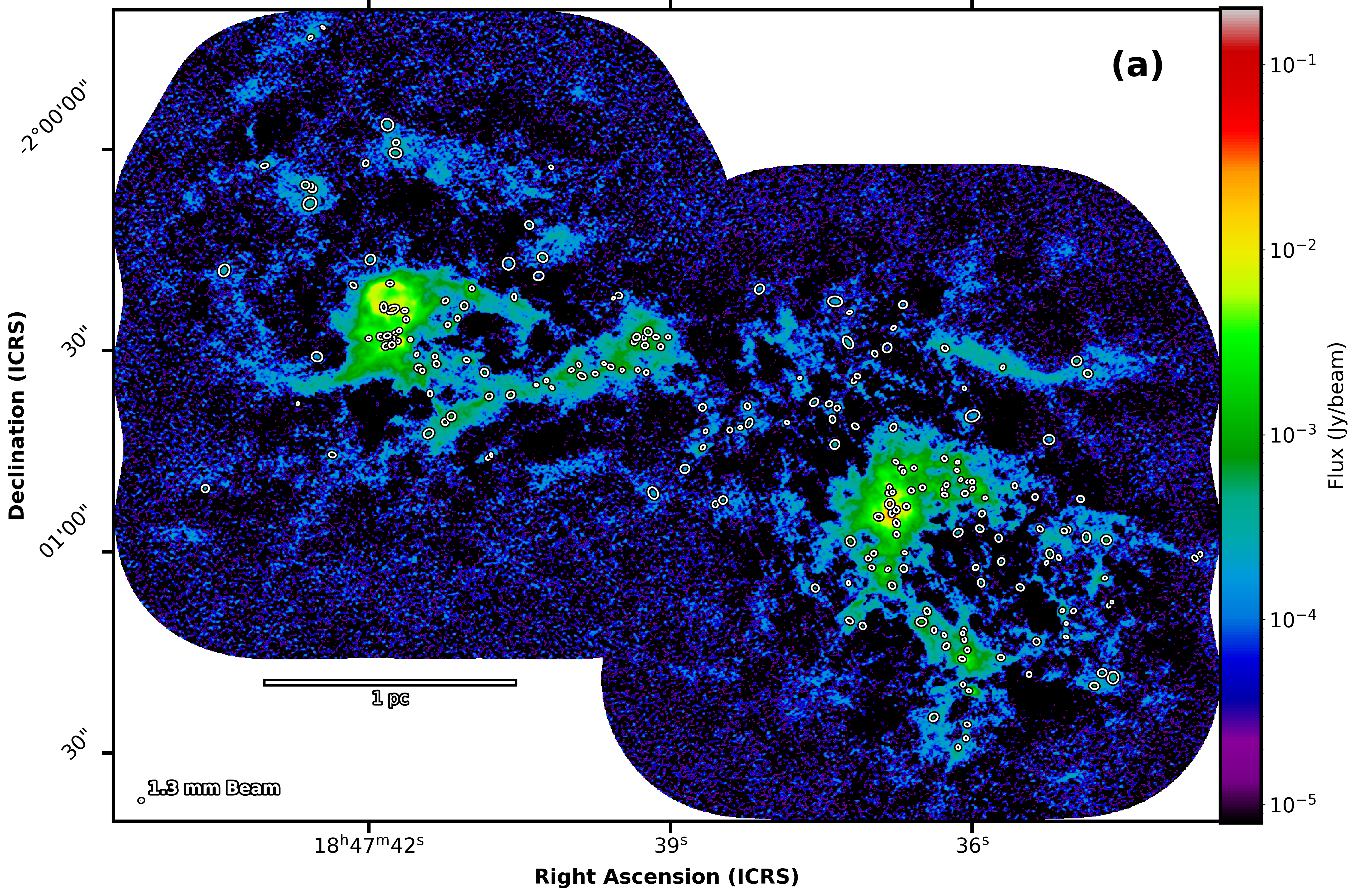
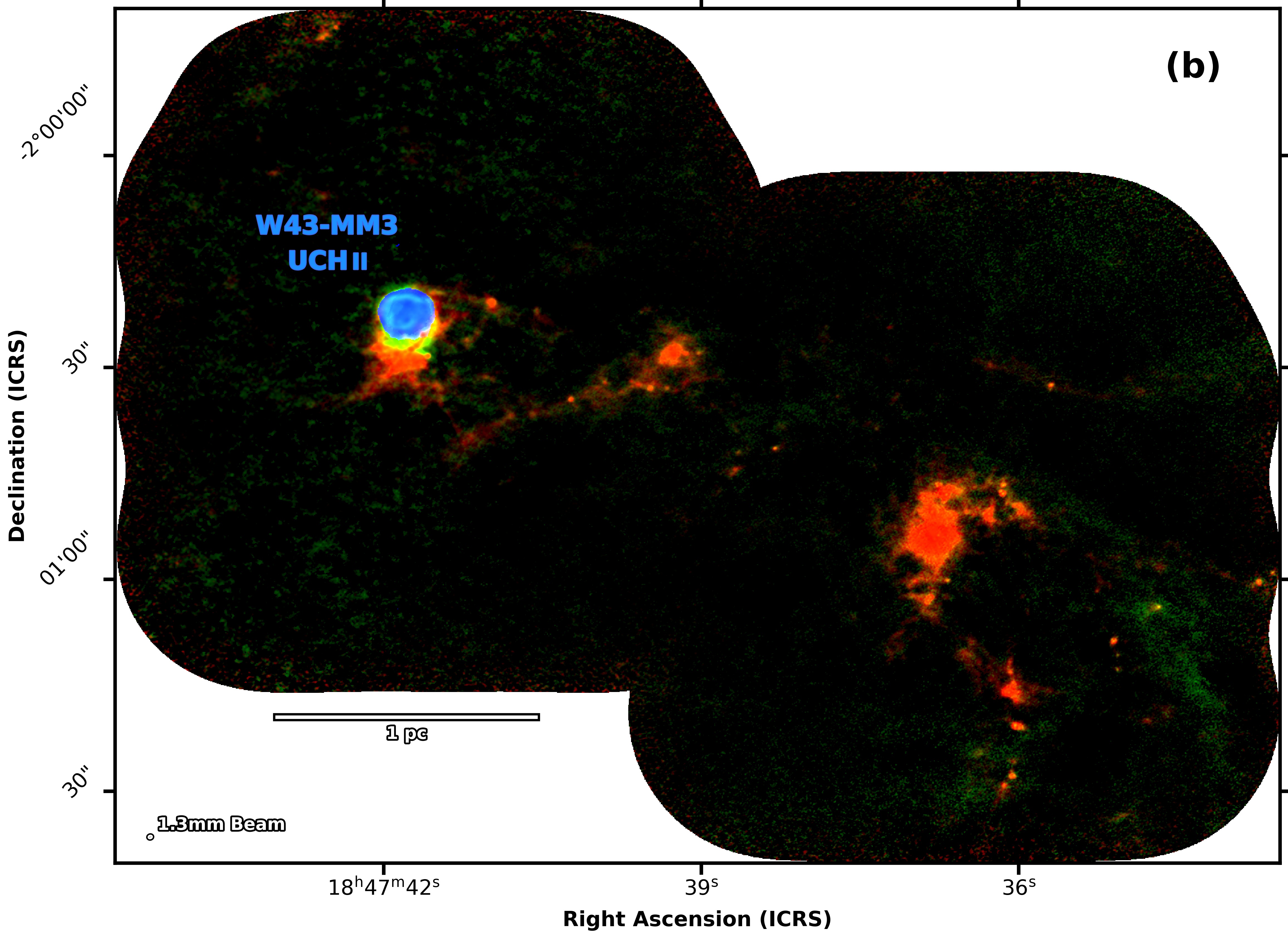
Figure 1: W43-MM2&MM3 protocluster cloud. Panel (a): 1.3 mm image obtain by the ALMA 12 m array (best-sensitivity image, prior to primary-beam correction). W43-MM2 is to the west and W43-MM3 is to the east. White ellipses outline the FWHM size of compact cores extracted by getsf. Panel (b): Three-color ALMA image. Red and green display the bsens continuum images at 1.3 mm and 3 mm, respectively, scaled by the theoretical ratio of thermal dust emission (see Eq. 3). Blue corresponds to the free-free continuum emission image at the frequency of the H41$\alpha$ recombination line (Galván-Madrid et al. in prep.). Filaments and cores appear in orange (red $+$ green), tracing thermal dust emission; the UCH ii region appears in blue or cyan (blue $+$ green), indicating free-free emission. Ellipses in the lower left corners represent the angular resolution of the bsens 1.3 mm image and scale bars indicate the size in physical units.

The ALMA-IMF pipeline produces two different estimates of the continuum images (see Ginsburg et al. 2021). The first, called the cleanest image, was produced using the findContinuum routine of CASA which excludes, before the TCLEAN task, the channels associated with lines to estimate the continuum level. The cleanest image is thus a continuum image free of line contamination. In the case of the ALMA-IMF data of W43-MM2 and W43-MM3, the bandwidths of the cleanest images are, respectively, a fraction of $\sim$50% and $\sim$90% of the total bandwidths at 1.3 mm and 3 mm (see Table 1 and Fig. 3 of Ginsburg et al. 2021). The second continuum image produced by the ALMA-IMF pipeline uses all channels of all the spectral bands to estimate the continuum at 1.3 mm and 3 mm. With a $\sim$30% decrease in the rms noise level, it corresponds to the best-sensitivity image and is thus called the bsens image (see Table 1).

The W43-MM2 and W43-MM3 ALMA fields share a common area in both bands: $\sim$10$\arcsec\times 90\arcsec$ at 1.3 mm and $\sim$100$\arcsec\times 180\arcsec$ at 3 mm within their respective primary-beam responses down to 15%. We combined the individually cleaned images in the image plane because CASA 5.4 cannot clean two fields with two different phase centers using the multiscale option. Although we requested the same angular resolution for both 1.3 mm and 3 mm mosaics, the latter were observed at a much higher resolution (see Table 1). We thus smoothed the W43-MM2 and W43-MM3 cleanest and bsens images at 3 mm to the angular resolution of the 1.3 mm images, $\sim$0.46$\arcsec$, or 2 500 au at the 5.5 kpc distance of W43. Because the beam orientations are similar (see Table 1), we assumed that the median of the W43-MM2 and W43-MM3 parallactic angles are good approximations for the beams of the combined images. We then used the primary-beam shape of each individual mosaic to weight the flux of pixels in the common area and define the combined primary-beam corrected image. This approach is valid because the noise level, when measured in the common area of maps with the same beam and uncorrected by the primary beam, is similar to within 20% between maps, which is smaller than the 35% difference measured on the whole map (see Table 1).

Figures 1a and 14 present the W43-MM2&MM3 ridge, covered by the combined image of the W43-MM2 and W43-MM3 protoclusters observed by ALMA-IMF. They display the 12 m array bsens image at 1.3 mm and 3 mm, respectively. Figure 1b presents a three-color image, which separates the thermal dust emission of star-forming filaments from the free-free emission associated with H ii regions, as done in Paper I (Motte et al. 2021). It uses ALMA-IMF images of the 1.3 mm and 3 mm continuum and of the H41$\alpha$ recombination line, tracing the free-free continuum emission of ionized gas (see Sect. 2 and Motte et al. 2021). Several filaments cross the image and the W43-MM2 cloud displays a centrally concentrated structure reminiscent of hubs (e.g., Myers 2009; Peretto et al. 2013; Didelon et al. 2015). In single-dish studies, W43-MM2 has a $2.4\times 10^{4}\leavevmode\nobreak\ L_{\odot}$ bolometric luminosity, integrated over 0.23 pc, and coincides with a 6.67 GHz methanol maser (Walsh et al. 1998; Motte et al. 2003). The W43-MM3 clump, itself characterized by Elia et al. (2021), has a 0.24 pc size and $5.7\times 10^{4}\leavevmode\nobreak\ L_{\odot}$ bolometric luminosity. In Fig. 1b, it harbors an ultra-compact H ii (UCH ii) region, whose bubble forms a ring-like structure. Its $\sim$0.12 pc diameter, or $\sim$4.8$\arcsec$ at 5.5 kpc, is in good agreement with its size estimated from single-dish millimeter continuum (Motte et al. 2003). Many compact sources are found along the dust emission of filaments of the W43-MM2&MM3 ridge, suggesting that they could be dense cloud fragments such as cores.

3 Extraction of compact sources

Since our goal is to extract cores from their surrounding cloud, we need to use software packages that identify and characterize cores as emission peaks, whose size is limited by their structured background and neighboring cores. Many source extraction algorithms have been used in star formation studies (see Joncour et al. 2020; Men’shchikov 2021). Here we use two completely independent methods, getsf and GExt2D.

The getsf method (Men’shchikov 2021) employs a spatial decomposition of the observed images to better isolate various spatial scales and separate the structural components of relatively round sources and elongated filaments from each other and from the background. The new method has many common features with its predecessors getsources, getfilaments, and getimages (Men’shchikov et al. 2012; Men’shchikov 2013, 2017). It has a single free parameter, the maximum size of the sources to be extracted. The detection provides a first-order estimate of the source footprints, sizes, and fluxes. As a second step, robust measurements of the sizes and fluxes of sources are done on background-subtracted images computed at each wavelength and, possibly, on other auxiliary images. The resulting catalog contains the size and fluxes of each source for each image.

GExt2D (Bontemps et al. in prep.), like the CuTeX algorithm (Molinari et al. 2017), uses second derivatives to identify the local maxima of the spatial curvature, which are then interpreted as the central positions of compact sources. The outskirts of each source are then determined, at each wavelength independently, from the inflexion points that are observed as the emission decreases away from the source peak. For each wavelength, the background under each source is evaluated by interpolating the emission along the source outskirts. Then, for all identified compact sources, their sizes and fluxes are measured by fitting Gaussians to their positions in the emission maps from which the associated background has been subtracted.

Both algorithms allow multiple input images and separate the source detection step (see Sect. 3.1) from the step that characterize the sources in terms of size and flux measurements (see Sect. 3.2).

3.1 Source detection

With the objective to build the most complete and most robust core catalog in the W43-MM2&MM3 protocluster cloud, the core positions and footprints should be defined in the detection image that provides the optimum image sensitivity. This corresponds to the bsens image at 1.3 mm (see Sect. 2). To further improve the sensitivity of the image chosen to detect cores, we removed the noise associated with cloud structures, which are incoherent from one scale to another. To do this we used the Multi-resolution non-Gaussian Segmentation software (MnGSeg) that separates the incoherent structures, referred to as Gaussian, of a cloud from the coherent structures associated with star formation (Robitaille et al. 2019, see also Appendix A). The removed Gaussian component corresponds to structural noise associated with the small-scale structures of cirrus that lie along the line of sight to the W43-MM2 and W43-MM3 protoclusters. In detail, the denoised image chosen for source extraction no longer contains incoherent components at scales larger than the beam size; it therefore consists of the sum of all the coherent cloud structures associated with star formation plus the white instrumental noise, which is a flux component needed to quantify the signal-to-noise ratio of extracted cores. We hereafter call denoised & bsens and denoised & cleanest the images passed through MnGSeg since their noise level decreases. As shown in Appendix A, images denoised by MnGSeg are indeed more sensitive and do not introduce spurious sources, meaning sources that are not part of the synthetic core population. In the case of the combined ALMA images of W43-MM2 and W43-MM3 the noise level decreased by about $\sim$30% at both 1.3 mm and 3 mm wavelengths (see Table 1), and thus allows the $5\,\sigma$ detection of point-like cores with masses of $\sim$0.20 $M_{\odot}$ (see Eq. 5 and adopted assumptions).

[c] Detection image cleanest bsens denoised & bsens Measurement images cleanest cleanest bsens denoised & cleanest denoised & bsens Number of sources, with robust 1.3 mm measurements^* 75 100 120 158 208 with measurable 3 mm fluxes^$\dagger$ 46 63 93 86 121

Table 2: Number of sources extracted by getsf in the W43-MM2&MM3 protocluster, using different detection images (all 12 m array 1.3 mm uncorrected by the primary beam) and various measurement images (all 12 m array 1.3 mm and 3 mm primary-beam-corrected).

• They are 1.3 mm sources that pass the recommended filtering of getsf: monochromatic goodness and significance above 1 in the detection image, small ellipticity, $a_{\rm 1.3mm}/b_{\rm 1.3mm}\leq 2$, and robust flux measurements at 1.3 mm, $S^{\rm peak}_{\rm 1.3mm}\geq 2\sigma^{\rm peak}_{\rm 1.3mm}$, and $S^{\rm int}_{\rm 1.3mm}\geq 2\sigma^{\rm int}_{\rm 1.3mm}$ in the measurement image. We also imposed a small average diameter, $\sqrt{a_{\rm 1.3mm}\times b_{\rm 1.3mm}}\leq 4\times\Theta_{\rm beam}$.

• The 3 mm fluxes of sources robustly detected at 1.3 mm are considered measurable when they correspond to small and low-ellipticity sources, $\sqrt{a_{\rm 3mm}\times b_{\rm 3mm}}\leq 4\times\Theta_{\rm beam}$ and $a_{\rm 3mm}/b_{\rm 3mm}\leq 2$, detected above $1\,\sigma_{\rm 3mm}$, $S^{\rm peak}_{\rm 3mm}>\sigma^{\rm peak}_{\rm 3mm}$, and $S^{\rm int}_{\rm 3mm}>\sigma^{\rm int}_{\rm 3mm}$.

Hereafter the master source catalogs will be those from the extraction performed with getsf (v210414), using the listed input images for the following:

• detection: 1.3 mm denoised & bsens 12 m array image, not corrected by the primary beam;

• 1.3 mm measurements: denoised & bsens and denoised & cleanest 12 m array images, corrected by the primary beam;

• 3 mm measurements: denoised & bsens and denoised & cleanest 12 m array images, corrected by the primary beam;

To facilitate core extraction, the noise level of the detection image is flattened, using images that are uncorrected by the primary beam. Table 6 lists the sources detected by getsf at 1.3 mm and identified by their peak coordinates, RA and Dec, along with their characteristics measured at 1.3 mm and at 3 mm in the denoised & bsens images: non-deconvolved major and minor diameters at half maximum, $a_{\rm 1.3mm}\times b_{\rm 1.3mm}$ and $a_{\rm 3mm}\times b_{\rm 3mm}$; position angles, PA_1.3mm and PA_3mm; peak and integrated fluxes, $S^{\rm peak}_{\rm 1.3mm}$, $S^{\rm peak}_{\rm 3mm}$, $S^{\rm int}_{\rm 1.3mm}$ and $S^{\rm int}_{\rm 3mm}$; two tags to identify cores also extracted by GExt2D and cores identified as suffering from line contamination (see Sect. 4.1.2). The getsf package extracted 208 cores that passed the basic recommended filtering (Men’shchikov 2021). Table 2 gives the number of sources extracted by getsf when using different detection and measurement images, from the cleanest to the bsens and finally denoised & bsens images, at 1.3 mm and 3 mm. The 208 sources of Table 6 are $\sim$1.6 times more numerous than the sources detected in the original & bsens image and $\sim$2.8 times more numerous that those detected in the original & cleanest image. In order to check the robustness of the getsf catalog of Table 6, GExt2D (v210208) is used. Applied to the bsens 12 m array 1.3 mm image, not corrected by the primary beam, and after the recommended post-filtering (Bontemps et al. in prep.), GExt2D provides a catalog of 152 cores.

3.2 Source characterization

The getsf and GExt2D measurements of source characteristics, that is to say their sizes and fluxes, were made in the 12 m array 1.3 mm and 3 mm images, which are primary-beam corrected. According to the good results of the MnGSeg denoising procedure applied on simulations of getsf extractions (see Appendix A), we kept the getsf measurements made in the denoised images. Since we need to estimate, and later on correct, the line contamination of fluxes of the sources extracted in the bsens image (see Sect. 4.1.2), extraction was performed in the denoised & cleanest images in addition to that performed in the denoised & bsens images. Using the maximum size free parameter of getsf, we excluded five sources with FWHM larger than four times the beam, $\sqrt{a_{\rm 1.3mm}\times b_{\rm 1.3mm}}>4\times\Theta_{\rm beam}$. They correspond to $\sim$10 000 au at $d=5.5$ kpc, which thus would be much larger than the typical core size expected to be a few 1 000 au in the dense W43 protoclusters (e.g., Bontemps et al. 2010; Palau et al. 2013; Motte et al. 2018b). They have low 1.3 mm fluxes, with a median mass of $\sim$2 $M_{\odot}$ (see Eq. 5), and are located at the outskirts of the protocluster cloud.

In summary, the getsf catalog of Table 6 contains 208 sources, which are detected at 1.3 mm with robust flux measurements. Given the lower sensitivity of our 3 mm continuum images, 121 have 3 mm fluxes that are qualified as “measurable” because they are above $1\,\sigma$ (see Table 2). Of the 208 getsf sources, 100 are qualified as “robust” because they are also identified by GExt2D and $\sim$90% of these common sources have no significant differences in their integrated fluxes, that is, their fluxes are at worst a factor of two larger or smaller than each other. The sources that have 1.3 mm fluxes consistent to within 30% are considered even more robust, as indicated in Table 6.

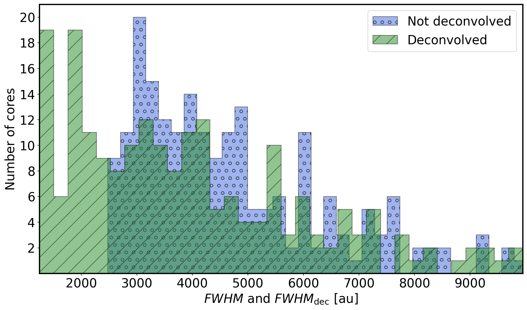
Figure 2: Distribution of the FWHM and FWHM^dec of the getsf sources as measured at 1.3 mm. A minimum size of $1\,300$ au is assumed for FWHM^dec. The median value of the core deconvolved sizes is about $0.75\arcsec\simeq 1.6\times\Theta_{\rm beam}$ with $\Theta_{\rm beam}=0.46\arcsec$, corresponding to $\sim$3 400 au.

Figure 2 displays, for the 208 sources extracted by getsf, histograms of their 1.3 mm physical sizes before and after beam deconvolution, FWHM$=\sqrt{a_{\rm 1.3mm}\times b_{\rm 1.3mm}}\times d$ and FWHM${}^{\rm dec}=\sqrt{a_{\rm 1.3mm}\times b_{\rm 1.3mm}-\Theta_{\rm beam}^{2}}\times d$, projected at the $d=5.5$ kpc distance of W43. The W43-MM2&MM3 compact sources have deconvolved sizes ranging from $\sim$1 300 au to $\sim$10 000 au with a median value of $\sim$3 400 au. Given their small physical sizes, these cloud fragments could represent the mass reservoirs, or at least the inner part of those reservoirs, that will undergo gravitational collapse to form a star or a small mutiple system. Following the classical terminology (e.g., Motte et al. 2018a) and if they are real cloud fragments (see Sect. 4.1), we hereafter call them cores.

4 Core nature and core mass estimates

Sources in the W43-MM2&MM3 protocluster are generally characterized from their measurements in the 1.3 mm denoised & bsens images obtained with the ALMA 12 m array (Table 6). Some of them, however, may not correspond to real cores or may have 1.3 mm denoised & bsens fluxes contaminated by line emission; their nature is investigated in Sect. 4.1. When the W43-MM2&MM3 core sample is cleaned and the 1.3 mm fluxes are corrected, core masses are estimated (see Sect. 4.2).

4.1 Core sample of the W43-MM2&MM3 ridge

To ensure that the millimeter sources of Table 6 are indeed dense cloud fragments and to correctly measure their mass, we investigated the contamination of their 1.3 mm and 3 mm continuum fluxes by free-free (see Sect. 4.1.1) and line emission (see Sect. 4.1.2). From the 208 sources of Table 6, we removed three sources which correspond to structures dominated by free-free emission and corrected the 1.3 mm measurements of 14 cores contaminated by line emission.

4.1.1 Correction for free-free contamination

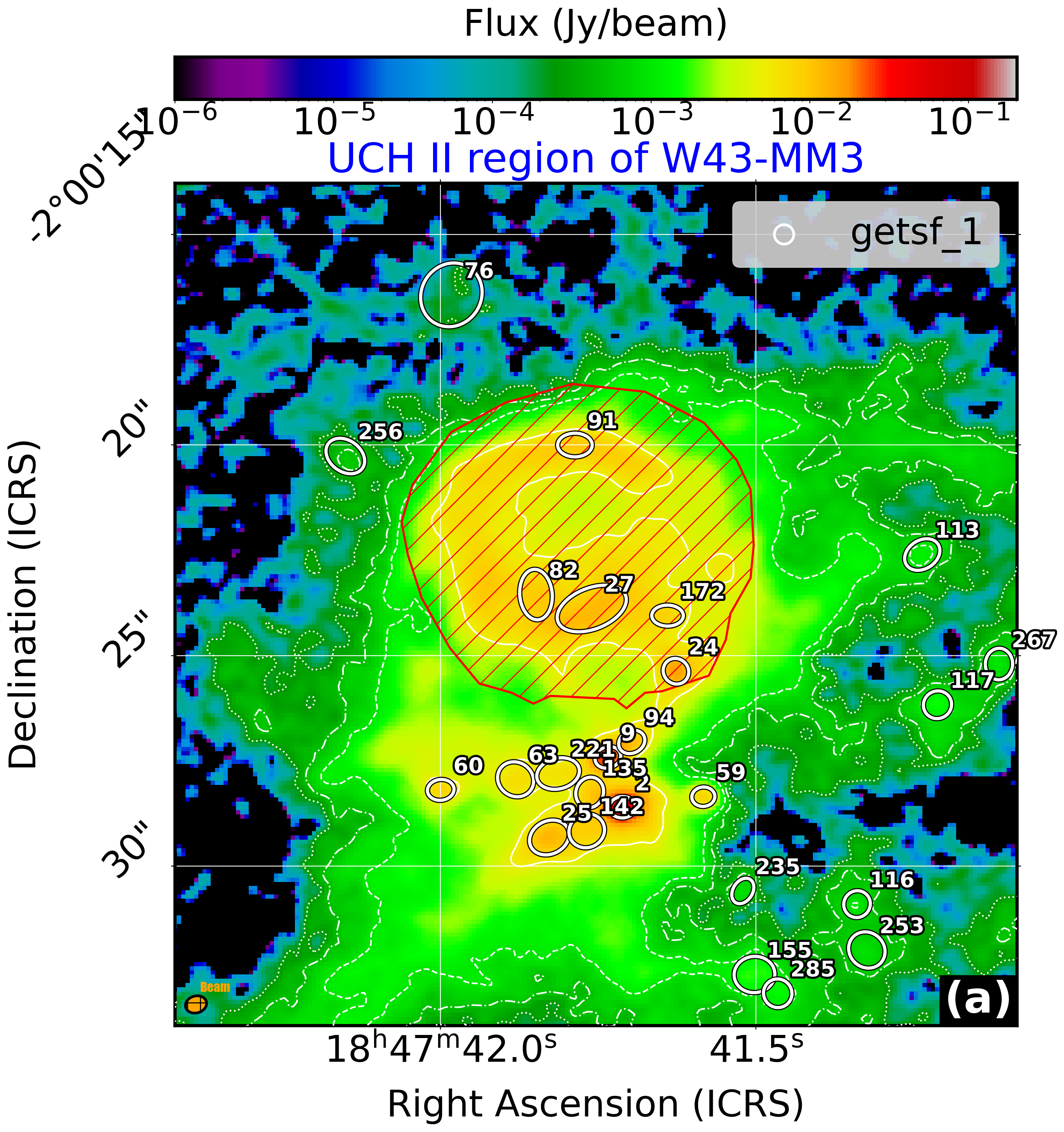
Figure 3: Investigating free-free contaminated sources. Panel (a): UCH ii region of W43-MM3 and its surrounding cloud imaged by ALMA at 1.3 mm. The red hatched region outlines the H41$\alpha$ recombination line emission of the H ii region. White ellipses outline source boundaries (at half maximum) as defined by getsf. Panel (b): Thermal dust emission cores separated from free-free emission sources, using their 1.3 mm to 3 mm flux ratios, $\gamma_{1}$, and shown as a function of the S/N in the 1.3 mm image. Blue points indicate cores with 3 mm thermal dust emission whose flux is rescaled to the source size measured at 1.3 mm (see Eq. 1), while orange points locate cores undetected at 3 mm, thus taking the ratio of the 1.3 mm peak flux to the $1\,\sigma$ peak error at 3 mm, corresponding to a lower limit. Red symbols are sources located within the H41$\alpha$ recombination line region displayed in panel (a). The gray curve indicates the median value of the core ratios, computed over bins of 20 adjacent cores as ranked by their S/N. The shaded gray area indicates the corresponding $3\,\sigma$ dispersion in flux ratio values. The magenta horizontal dashed line represents the theoretical flux ratio of thermal dust emission of 15.4, computed in Eq. 3. The red hatched area locates the theoretical flux ratios of UCH ii or HCH ii regions, whose free-free emission is either optically thin (lower limit) or partly to totally optically thick (upper limit).

Figure 1b shows that there is only one localized area associated with free-free emission in the 1.3 mm ALMA-IMF images of W43-MM2 and W43-MM3. This is the W43-MM3 UCH ii region which is particularly bright at 3 mm. Figure 3a displays the boundary of this H ii region, as defined by the H41$\alpha$ recombination line emission observed as part of the ALMA-IMF Large Program (Galván-Madrid et al. in prep.). In this area the large-scale continuum emission mainly consists of free-free emission, and the thermal dust emission of cores could only represent a minor part of the total flux at small scales. This calls into question the nature of the five compact sources detected over the extent of the H ii bubble that may not be interpreted as dust cores: #24, #27, #82, #91, and #172 (see Fig. 3a).

We investigated the free-free contamination of the cores of Table 6 by measuring the ratio of their 1.3 mm to 3 mm integrated fluxes, $S^{\rm int}_{\rm 1.3mm}$ and $S^{\rm int}_{\rm 3mm}$. To allow a direct comparison of these fluxes, not always integrated over the same area and thus not defining the same parcel of the cloud, we rescaled the 3 mm integrated flux of cores to their deconvolved 1.3 mm sizes, FWHM${}^{\rm dec}_{\rm 1.3mm}$. We assumed a linear relation between the integrated flux and the angular scale, $S^{\rm int}(\Theta)\propto\Theta$, corresponding to the optically thin emission of an isothermal, $T(r)\simeq\rm constant$, protostellar envelope with a $\rho(r)\propto r^{-2}$ density distribution (Motte & André 2001; Beuther et al. 2002).This flux rescaling was applied in Herschel studies that aimed to fit meaningful spectral energy distributions (Motte et al. 2010; Nguyen Luong et al. 2011a; Tigé et al. 2017). As discussed in Tigé et al. (2017), this correction factor would be larger for starless fragments that have a flatter density distribution, thus leading to a $S^{\rm int}(\Theta)\propto\Theta^{m}$ relation with $m>1$. In the case of hyper-compact H ii regions (HCH ii), potentially optically thick at their center, a larger correction factor would also be necessary. The rescaled 3 mm fluxes are computed via the following equation:

$$(S^{\rm int}_{\rm 3mm})^{\rm rescaled}_{m}=S^{\rm int}_{\rm 3mm}\times\left(\frac{{\rm FWHM}^{\rm dec}_{\rm 1.3mm}}{{\rm FWHM}^{\rm dec}_{\rm 3mm}}\right)^{m}.$$ (1)

Figure 3b displays, for the complete catalog of Table 6, the ratios of the 1.3 mm to 3 mm fluxes with a rescaling using $m=1$. On average, 3 mm fluxes are corrected by $25\%$, with a maximum of $75\%$, for the cores that have measurable fluxes both at 1.3 mm and 3 mm. For the many cores that remain undetected or that have barely measured fluxes at 3 mm, $S^{\rm int}_{\rm 3mm}\leq\sigma$, we used the $1\,\sigma$ rms noise level to give a lower limit of their 1.3 mm to 3 mm flux ratio, $\frac{S^{\rm int}_{\rm 1.3mm}}{S^{\rm int}_{\rm 3mm}}\geq\frac{S^{\rm peak}_{\rm 1.3mm}}{\sigma_{\rm 3mm}^{\rm peak}}$. In addition, Figs. 15a–b display the same figure without rescaling ($m=0$) and for a rescaling better suited for starless cores ($m=2$). Figures 3b and 15a–b allow a simple separation of sources dominated by thermal dust emission from those dominated by free-free emission. Under the optically thin assumption and arising from the same source area, the 1.3 mm to 3 mm theoretical flux ratio of thermal dust emission is given by

$$\gamma =\frac{S_{\rm 1.3mm}^{\rm int}}{S^{\rm int}_{\rm 3mm}}$$ (2)

$$=\frac{\kappa_{\rm 1.3mm}}{\kappa_{\rm 3mm}}\frac{B_{\rm 1.3mm}(T_{\rm dust})}{B_{\rm 3mm}(T_{\rm dust})}=\frac{\kappa_{\rm 1.3mm}}{\kappa_{\rm 3mm}}\frac{\nu_{\rm 1.3mm}^{3}}{\nu_{\rm 3mm}^{3}}\frac{e^{h\,\nu_{\rm 3mm}/k_{\rm B}\,T_{\rm dust}}-1}{e^{h\,\nu_{\rm 1.3mm}/k_{\rm B}\,T_{\rm dust}}-1}\simeq 15.4,$$ (3)

where $k_{\rm B}$ and $h$ are the Boltzmann and Planck constants, and $B_{\rm 1.3mm}(T_{\rm dust})$ and $B_{\rm 3mm}(T_{\rm dust})$ are the Planck function for the mean dust temperature of cores, $T_{\rm dust}=23$ K, at $\nu_{\rm 1.3mm}=228.9$ GHz and $\nu_{\rm 3mm}=100.7$ GHz. These frequency values are taken from Paper II (Ginsburg et al. 2021) assuming a spectral index of $\alpha(\nu)=3.5$, which corresponds to a dust opacity spectral index of $\beta=1.5$, suitable for optically thin dense gas at the core scale (see André et al. 1993; Juvela et al. 2015). Because the W43-MM2&MM3 ridge is a dense cloud (Nguyen Luong et al. 2013), we adopted a dust opacity per unit (gas $+$ dust) mass adapted for cold cloud structures: $\kappa_{\rm 1.3mm}=0.01\,\rm cm\,g^{-1}$ (Ossenkopf & Henning 1994). The dust opacity mass at 3 mm, $\kappa_{\rm 3mm}$, is computed assuming

$$\kappa_{\lambda}=0.01\times\left(\frac{\lambda}{\rm 1.3\,mm}\right)^{-\beta}=0.01\times\left(\frac{\nu}{\rm 228.9\,GHz}\right)^{\beta}\leavevmode\nobreak\ \rm cm^{2}\,g^{-1}$$ (4)

with $\beta=1.5$. For the cores that remain after post-filtering at both wavelengths, we computed their ratio of 1.3 mm flux to 3 mm flux, which is rescaled to the 1.3 mm size with an index of either $m=1$ or $m=2$ (see Eqs. 1–2): $\gamma_{1}=\gamma^{\rm rescaled}_{m=1}$ and $\gamma_{2}=\gamma^{\rm rescaled}_{m=2}$, respectively. They have a median 1.3 mm to 3 mm flux ratio and associated standard deviation of $\widetilde{\gamma_{1}}\simeq 11.3\pm 1.8$ (see Fig. 3b), which is close to the expected value of 15.4 (see Eq. 3). Figure 3b shows that the 1.3 mm to 3 mm flux ratio tends to increase as the signal-to-noise ratio (S/N) increases, equivalent to the core flux increases. Rescaling the fluxes with an index of $m=2$, rather than $m=1$, removes this unexpected correlation and leads to a median flux ratio of $\widetilde{\gamma_{2}}\simeq 15.3\pm 2.0$ (see Fig. 15a), which is closer to the theoretical value (see Eq. 3). If confirmed, this result would argue in favor of the pre-stellar rather than protostellar nature of most of the cores extracted in the W43-MM2&MM3 protoclusters. A companion paper by Nony et al. (in prep.) consistently shows that the protostellar to pre-stellar ratio of the W43-MM2&MM3 core sample is about $\sim$25%.

In contrast, the 1.3 mm to 3 mm flux ratio of free-free emission is expected to be much lower than the ratio of thermal dust continuum emission estimated in Eq. 3. With a spectral index of optically thin and optically thick free-free emission of $\alpha(\nu)=-0.1$ and $\alpha(\nu)\simeq 2$ (e.g., Keto et al. 2008), respectively, the theoretical 1.3 mm to 3 mm flux ratios for H ii regions lie within the $\simeq$0.9–5.2 range. As shown in Fig. 3a, we found that

• three sources have low ratios ($\gamma_{1}\simeq 0.9$) and are located along the H ii ring within the free-free continuum bubble of W43-MM3. Sources #27, #82, and #91 most likely correspond to free-free emission fluctuations in the UCH ii region.

• source #24, which is located over the UCH ii region extent, has a high 1.3 mm to 3 mm flux ratio, $\gamma_{1}\simeq 18$, and can thus be considered a true core that is dominated by dust emission and lies on the same line of sight as the UCH ii region (see Figs. 3a–b).

• we find 13 sources in Fig. 3b that have an intermediate flux ratio, $\gamma_{1}\simeq 1.2-5$, and may indicate that they consist of partially optically thick free-free emission. However, only one source (source #172) lies within the W43-MM3 H ii bubble, and it has a lower-limit ratio of $\gamma_{1}\geq 5$. Moreover, none of the sources with $\gamma_{1}=1.2-5$ ratios is associated with strong H41$\alpha$ recombination line emission, as expected for most HCH ii regions. We therefore considered them to be real cores.

To confirm this, we developed a methodology that better takes into account the uncertainties of our source extraction and flux measurement process. For the 121 dust cores detected at 1.3 mm and that have measurable 3 mm fluxes, Figs. 3b and 15 locate the $3\,\sigma$ dispersion zone of the logarithm of their flux ratios. None of these sources with $\gamma_{1}=1.2-5$ ratios lie outside this $3\,\sigma$ zone, suggesting that their flux measurements are too uncertain to securely qualify these sources as being free-free emission peaks.

In summary, Fig. 3b, Figs. 15a–b, and the same figures done for peak fluxes, identified only three sources that likely correspond to free-free emission peaks: #27, #82, and #91. Table 6 pinpoints these three sources; they are removed from the core sample of Table 7 and will not be considered further.

4.1.2 Correction for line contamination

In order to correctly measure the mass of cores, it is necessary to correct their continuum flux for line contamination. The 1.3 mm and 3 mm denoised & bsens images used to identify sources in Sect. 3 indeed provide estimates of their continuum emission, based on all channels of all spectral bands. Some of these bands, however, contain bright emission lines associated with dense gas (see, e.g., Table 3 of Motte et al. 2021). In addition, line forests of complex organic molecules (COMs; e.g., Garrod & Herbst 2006) are expected in all spectral windows when observing hot cores and shocked regions (e.g., Molet et al. 2019; Bonfand et al. 2019). Investigating the contamination by lines of the bsens continuum can be done by comparing bsens fluxes to fluxes measured in the cleanest images (see Motte et al. 2018b).

Figure 4 presents, for the 155 sources at 1.3 mm with robust denoised & bsens and cleanest fluxes, the ratios of their denoised & bsens to their cleanest 1.3 mm peak fluxes. We use the peak rather than the integrated flux because the vast majority of hot cores are expected to be unresolved, and therefore have a higher ratio of denoised & bsens to cleanest peak fluxes. Most sources have ratios that remain close to $1$, with a decrease in the point dispersion as the S/N of the denoised & cleanest fluxes increases (see Fig. 4). As in Fig. 3b, we computed the $3\,\sigma$ dispersion zone of the plotted flux ratios and found that

• four of the brightest sources (S/N $>20$) that lie above this $3\,\sigma$ zone have been identified as candidates to host a hot core by Herpin et al. (in prep.), namely cores #1, #3, #7, and #10. The line contamination of their 1.3 mm denoised & bsens peak flux is estimated to range from 20% to 45% (see Fig. 4).

• ten other sources lie well above the $3\,\sigma$ dispersion zone with high flux ratios, $\frac{(S_{\rm 1.3mm}^{\rm peak})_{\rm bsens}}{(S_{\rm 1.3mm}^{\rm peak})_{\rm cleanest}}=2-12$, seven of which (#46, #47, #85, #114, #152, #224, and #245) correspond to sources contaminated by the ¹²CO(2-1) line, which present an excess of flux in the continuum emission of the denoised & bsens image. The three remaining sources (#183, #248, and #275) are most probably contaminated by other lines, undetermined at this stage.

As indicated in Table 7, the properties of these four and ten cores are derived from their measurements in the denoised & cleanest image. Given that we could only investigate the line contamination of 155 out of 205 sources, we expect to have, in our core catalog of Table 7, a maximum of four that have core masses overestimated sources in the $0.1-0.5$ $M_{\odot}$ mass range.

In summary, from the 208 sources of Table 6, we removed three sources, that correspond to structures dominated by free-free emission (see contamination tag). For the 14 cores contaminated by line emission (see Table 6), we corrected their 1.3 mm measurements, including size and fluxes, by taking their denoised & cleanest measurements.

Figure 4: Line contamination of the 1.3 mm continuum fluxes of getsf sources, as estimated from the ratio of denoised & bsens to cleanest peak fluxes, and shown as a function of the S/N in the cleanest image. The gray curve indicates the median value of the core ratios, computed over bins of 20 adjacent cores as ranked by their S/N. The shaded gray area indicates the corresponding $3\,\sigma$ dispersion in flux ratio values. The red, orange, and green points locate cores with hot-core signatures (Herpin et al. in prep.), cores contaminated by the CO(2-1) line, and cores contaminated by other spectral lines, respectively. The horizontal lines indicate the contamination levels of 0% (magenta dashed line) and 20% (green dotted line). By taking only the blue points, the denoised & bsens over cleanest ratios of Fig. 4 have a median value of $\simeq 1.1\pm 0.3$.

4.2 Mass estimates

We estimate the masses of cores, which are extracted by getsf in Sect. 3 and listed in Table 7. Because the thermal dust emission of cores is mostly optically thin at 1.3 mm, one generally uses the classical optically thin equation is genrally used to compute their masses. We give it here and provide a numerical application whose dependence on each physical variable is given, for simplicity, in the Rayleigh-Jeans approximation:

$$\begin{split}M_{\rm\tau\ll 1}\>&=\frac{S^{\rm int}_{\rm 1.3\,mm}\;d^{2}}{\kappa_{\rm 1.3\,mm}\;B_{\rm 1.3\,mm}(T_{\rm dust})}\\ &\simeq\>5\,M_{\odot}\times\left(\frac{S^{\rm int}_{\rm 1.3\,mm}}{\mbox{10\leavevmode\nobreak\ mJy}}\right)\left(\frac{T_{\rm dust}}{\rm 23\leavevmode\nobreak\ K}\right)^{-1}\\ &\leavevmode\nobreak\ \leavevmode\nobreak\ \leavevmode\nobreak\ \leavevmode\nobreak\ \times\left(\frac{d}{\mbox{5.5\leavevmode\nobreak\ kpc}}\right)^{2}\left(\frac{\kappa_{\rm 1.3\,mm}}{\rm 0.01\,cm^{2}\,g^{-1}}\right)^{-1}.\end{split}$$ (5)

We estimated the volume-averaged core temperatures, $T_{\rm dust}$, from a map that combines a moderate angular resolution dust temperature image with the central heating and self-shielding of protostellar and pre-stellar cores, respectively (see Fig. 16 and Motte et al. in prep.). The dust temperature image is produced by the Bayesian fit of spectral energy distributions, performed by the PPMAP procedure (Marsh et al. 2015). Using the five Herschel $70-500\leavevmode\nobreak\ \mu$m images, two APEX 350 and 870 $\mu$m images, and the present ALMA 1.3 mm image, which have a large range of angular resolutions ($0.46\arcsec-36\arcsec$), provides a $2.5\arcsec$-resolution dust temperature image that needs to be extrapolated to the $0.46\arcsec$ resolution of our 1.3 mm ALMA-IMF image. The dust temperature of the immediate background of cores listed in Table 7 has a mean value of $\overline{T_{\rm dust}}^{\rm core\,bkg}=24\pm 2$ K. Following Motte et al. (2018b), the dust temperature of massive protostellar cores averaged in $0.46\arcsec$-resolution elements is estimated from the total luminosity of the W43-MM2 cloud ($\sim$$2\times 10^{4}\leavevmode\nobreak\ L_{\odot}$, Motte et al. 2003) divided between cores, in proportion to their associated line contamination in the 1.3 mm band (see Motte et al. in prep.). This leads to volume-averaged temperatures, $T_{\rm dust}$, between 20 K and 65 K. In addition, the mean core temperature of lower-mass cores driving outflows (see Nony et al. in prep.) is increased by $4\pm 4$ K compared to the core background temperature. The temperature of candidate pre-stellar cores is itself decreased by $2\pm 2$ K compared to their background temperature. The resulting estimates of the mass-averaged temperature of cores range from 19 K to 65 K, with uncertainties ranging from $\pm 2$ K to $\pm 10$ K (see Table 7).

For the cores that reach sufficiently high densities ($\gtrsim 5\times 10^{7}$ cm^-3, see Eq. 7), in other words the most massive ones, we expect them to be optically thick (e.g., Cyganowski et al. 2017; Motte et al. 2018a). To partly correct for this opacity, Motte et al. (2018a) proposed an equation, which is given below and fully explained in Appendix B:

$$M_{\rm\tau\gtrsim 1}\>=-\,\frac{\Omega_{\rm beam}\;d^{2}}{\kappa_{1.3{\rm mm}}}\,\frac{S^{\rm int}_{1.3{\rm mm}}}{S^{\rm peak}_{1.3{\rm mm}}}\,\ln\left(1\,-\,\frac{S^{\rm peak}_{1.3{\rm mm}}}{\Omega_{\rm beam}\;B_{1.3{\rm mm}}(T_{\rm dust})}\right).$$ (6)

Here $\Omega_{\rm beam}$ is the solid angle of the beam. This correction is significant for two cores (cores #1 and #2), whose masses estimated with the optically thin assumption would have been underestimated by $\sim$15%. With this correction of optical thickness and the temperatures estimated in Fig. 16, the core mass range is $0.1-70\leavevmode\nobreak\ M_{\odot}$ (see Table 3). To start estimating which of these cores are gravitationally bound, we compared the measured masses with virial masses. The core virial masses were calculated from their FWHM sizes measured at 1.3 mm and their estimated temperatures, $T_{\rm dust}$, given in Table 7. All the W43-MM2&MM3 cores could be gravitationally bound because their virial parameter, $\alpha_{\rm vir}=M_{\rm vir}/M_{\rm\tau\gtrsim 1}$, is always smaller than the factor 2 chosen by Bertoldi & McKee (1992) to define self-gravitating objects. Their dynamical state, however, requires further study of the non-thermal motions of the cores, which will be measured in part by future ALMA-IMF studies of spectral lines.

We estimated the absolute values of the core masses to be uncertain by a factor of a few, and the relative values between cores to be uncertain by $\sim$50%. Dust opacity should indeed evolve as the core grows and the protostar heats up (Ossenkopf & Henning 1994) and may also have a radial dependence from the core surroundings to its center. We therefore assumed a $1\,\sigma$ uncertainty for the dust opacity that should cover its variations with gas density and temperature; divided or multiplied by a factor of 1.5 it becomes $\kappa_{\rm 1.3mm}=0.01\pm^{0.005}_{0.0033}\,\rm cm\,g^{-1}$.

Table 7 lists the physical properties of the 205 cores derived from their 1.3 mm denoised & bsens measurements and the analysis made in Sect. 4: deconvolved size, FWHM^dec; mass corrected for optical depth, $M_{\rm\tau\gtrsim 1}$; dust temperature, $T_{\rm dust}$; volume density, $n_{\rm H_{2}}$. Volume densities are computed assuming a spherical core:

$$\begin{split}n_{\rm H_{2}}&=\frac{M_{\rm\tau\gtrsim 1}}{\frac{4}{3}\pi\,\mu\,m_{\rm H}\,\left({\rm FWHM}^{\rm dec}_{\rm 1.3mm}\right)^{3}}\\ &\simeq 7.8\times 10^{7}\,{\rm cm}^{-3}\times\left(\frac{M_{\rm\tau\gtrsim 1}}{\mbox{70\leavevmode\nobreak\ $M_{\odot}$}}\right)\left(\frac{{\rm FWHM}^{\rm dec}_{\rm 1.3mm}}{\mbox{3\,000\leavevmode\nobreak\ au}}\right)^{-3}.\end{split}$$ (7)

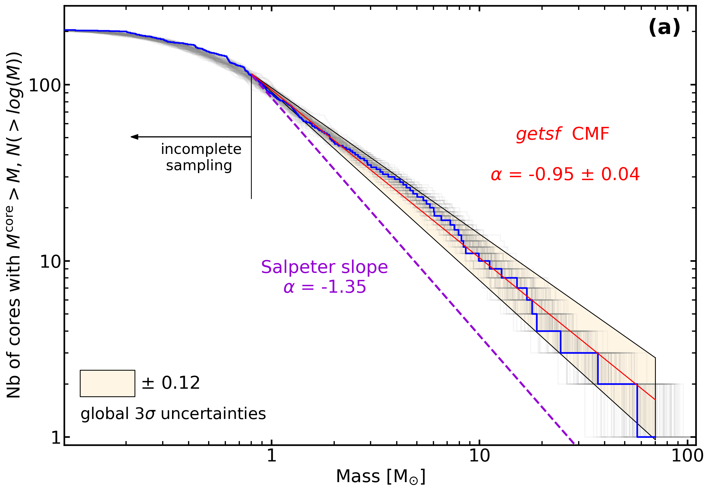
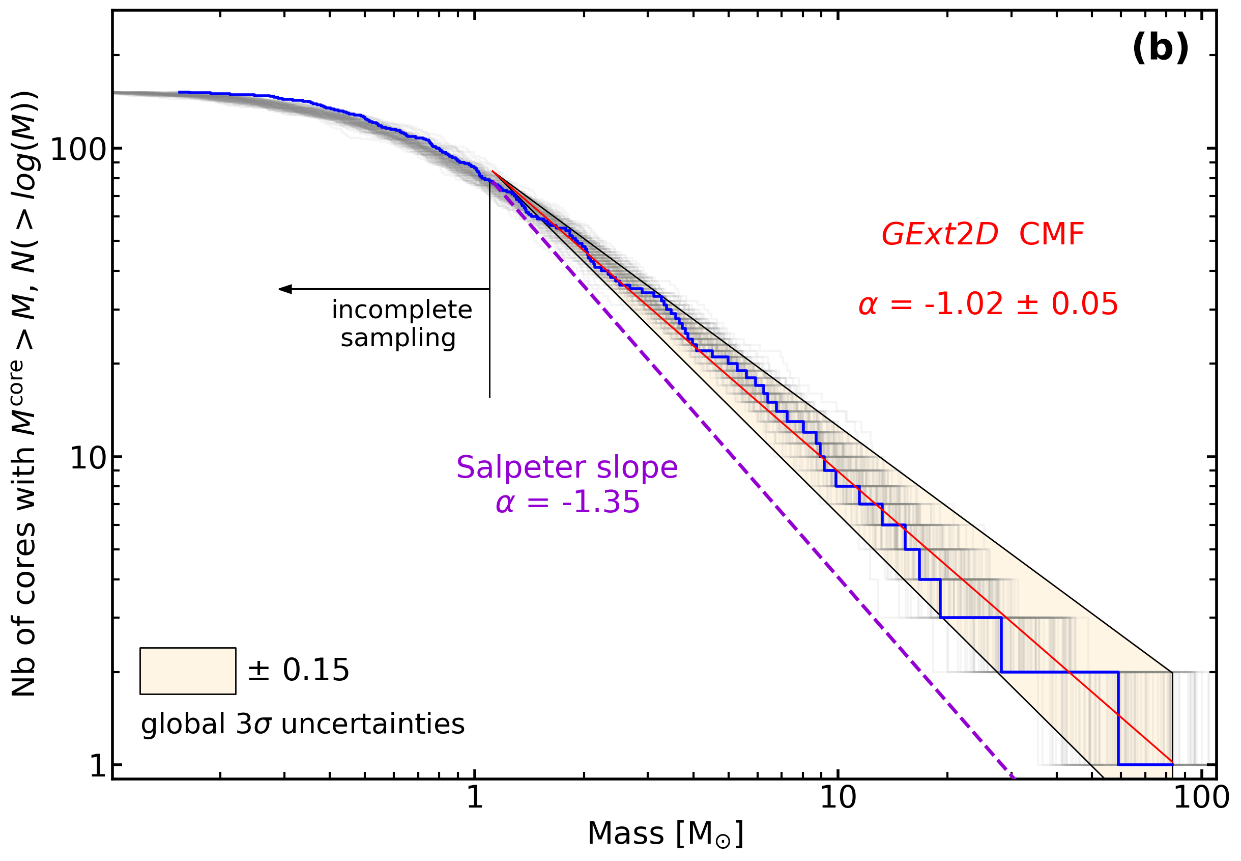
Figure 5: Top-heavy CMF of the W43-MM2&MM3 ridge, with cores extracted by the getsf (panel a) and GExt2D (panel b) software packages, in the denoised & bsens and original & bsens images, respectively. The cumulative forms of CMFs (blue histograms) are fitted above their 90% completeness levels (black vertical lines) by single power-laws of the form $N(>\log M)\propto M^{\alpha}$, with $\alpha=-0.95\pm 0.04$ (a) and $\alpha=-1.02\pm 0.05$ (b) (red lines and $1\,\sigma$ global uncertainties). The global $3\,\sigma$ uncertainties are computed from 2 000 CMFs that are uniformly randomly generated (light gray histograms) and from the fit uncertainty (see Sect. 5.1). The W43-MM2&MM3 CMF slope is clearly shallower than the high-mass end of the canonical IMF, which has a power-law index of $\alpha=-1.35$ (Salpeter 1955, dashed magenta lines).

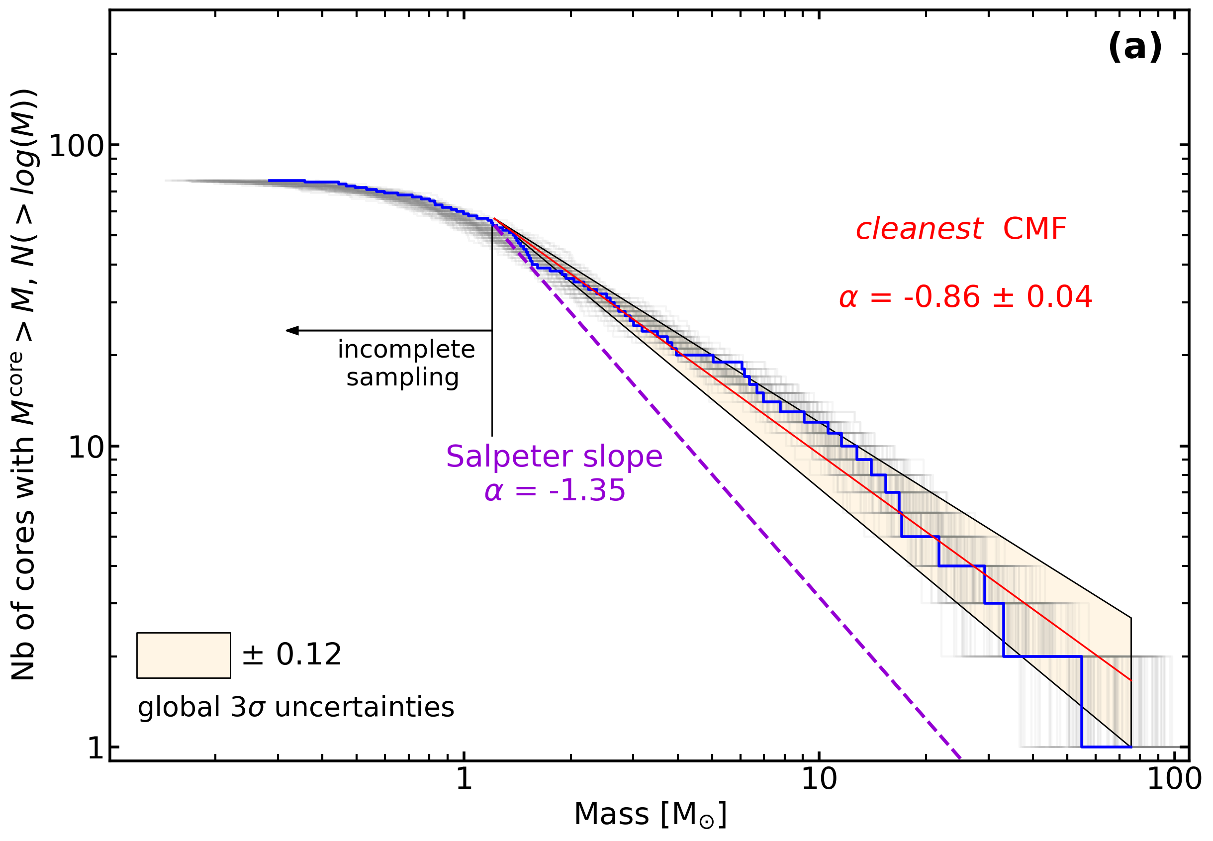
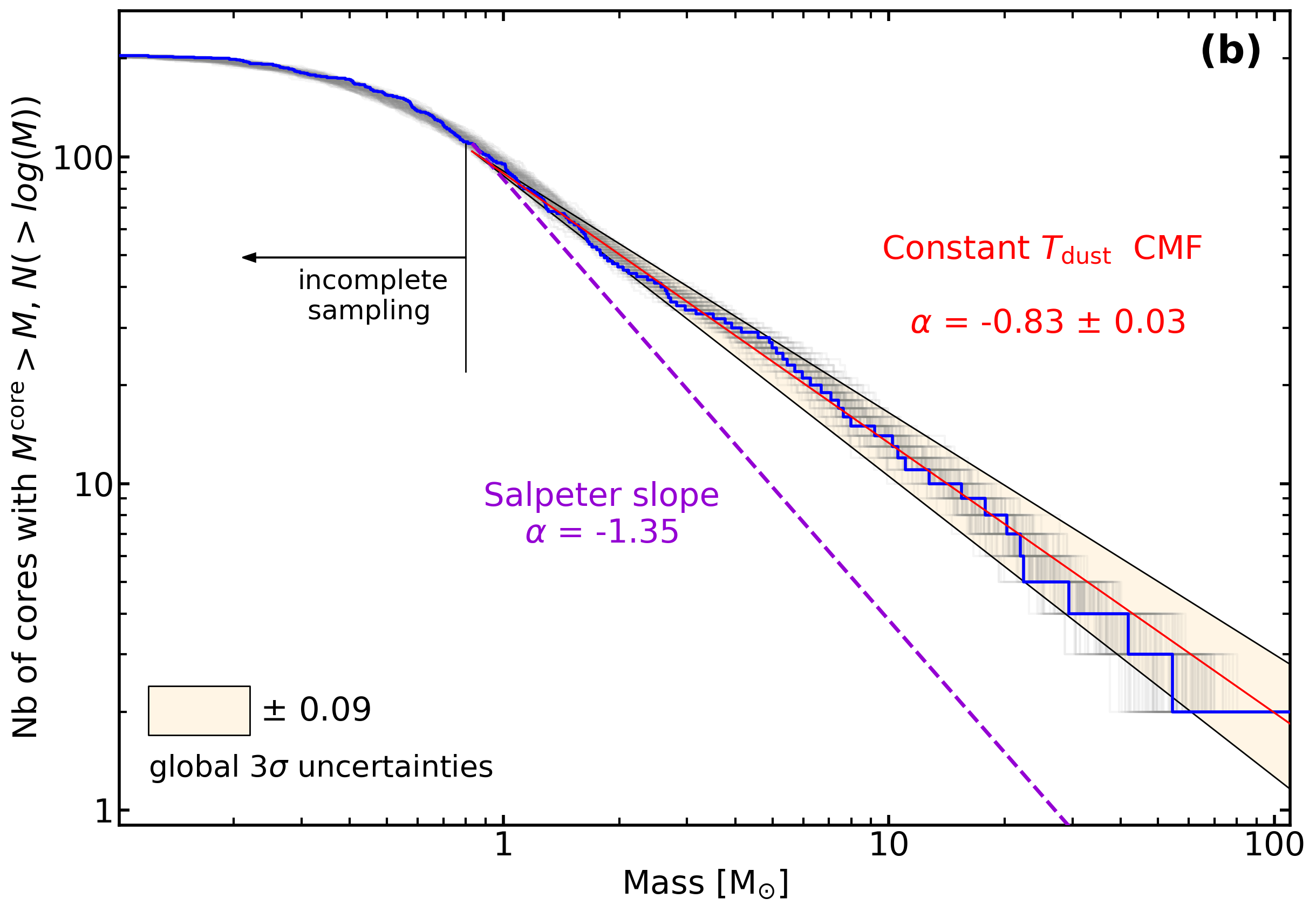
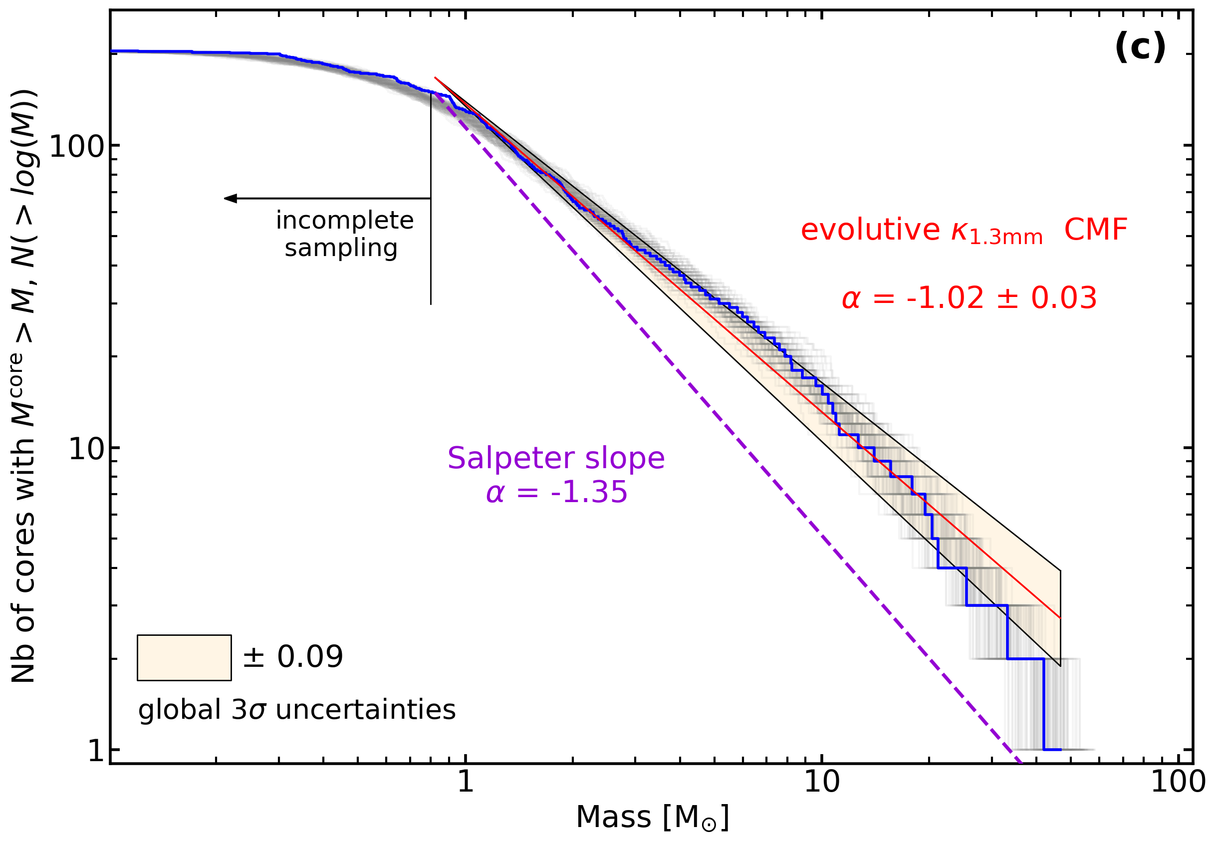
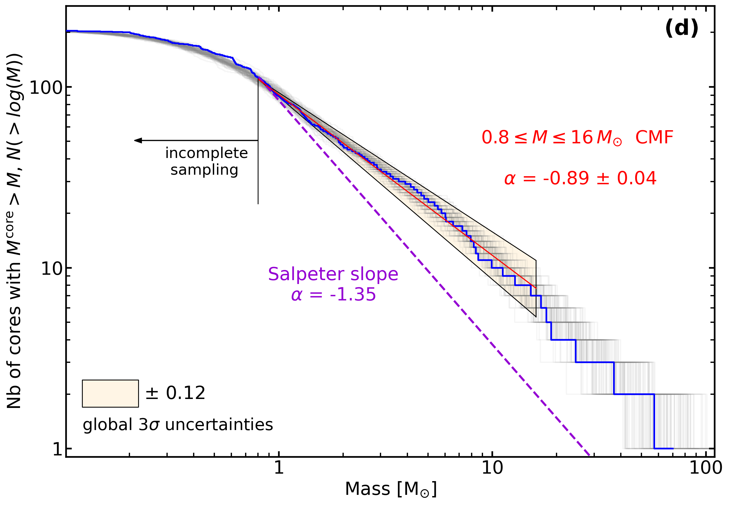
Figure 6: getsf CMFs of the W43-MM2&MM3 ridge built for a different core catalog (a), under different assumptions of dust temperature and emissivity (b and c), and fit over a different mass range (d). The cumulative CMFs, their completeness levels, power-law fits, global $3\,\sigma$ uncertainties (explained in Sect. 5.1), and the Salpeter slope of the canonical IMF are represented as in Fig. 5. Panel (a): CMF derived from the core catalog of Paper V (Louvet et al. in prep.), itself obtained by getsf extraction in the original & cleanest images of W43-MM2 and W43-MM3, showing a similar but slightly shallower slope of $\alpha=0.86\pm 0.04$. Panel (b): CMF obtained with a mean $T_{\rm dust}=23$ K dust temperature for all cores, instead of T_dust in Fig. 16, displaying a similar but slightly shallower slope of $\alpha=-0.83\pm 0.03$. Panel (c): CMF derived assuming a linear relation for the dust opacity with core mass (see Sect. 5.2) showing a steeper slope of $\alpha=-1.02\pm 0.03$. Panel (d): Fitting the CMF of Fig. 5a in the low- to intermediate-mass range,$0.8-16\leavevmode\nobreak\ M_{\odot}$. This leads to a similar but slightly shallower slope of $\alpha=-0.89\pm 0.04$.

[c]

Table 3: W43-MM2&MM3 core populations and CMF parameters, as derived by two core extraction algorithms.

Extraction	Number	$\sum M_{\rm\tau\lesssim 1}$	Mass range	$\alpha$
packages	of cores
		[$M_{\odot}$]	[$M_{\odot}$]
(1)	(2)	(3)	(4)	(5)
			$0.8-69.9$	$-0.95\pm 0.04$
getsf	205	$541\pm 29$	$0.8-16$	$-0.89\pm 0.04$
			$2.0-69.9$	$-1.05\pm 0.06$
			$1.1-83.1$	$-1.02\pm 0.05$
GExt2D	152	$468\pm 35$	$1.1-16$	$-0.98\pm 0.06$
			$2.0-83.1$	$-1.07\pm 0.07$

• (3) Cumulative mass of cores, listed in Table 7. Uncertainties arise from those associated with individual core mass estimates.

• (4) Mass range used to fit a power-law to the cumulative form of the CMFs. The lower limit of this mass range is the 90% completeness limit (see Appendix C and Sect. 5.1) of $2\leavevmode\nobreak\ M_{\odot}$; its upper limit corresponds to the maximum core mass detected or $16\leavevmode\nobreak\ M_{\odot}$.

• (5) Power law index of the CMFs in their cumulative form, $N(>\log M)\propto M^{\alpha}$. Uncertainties are estimated by varying dust temperature and emissivity and by taking into account the fit uncertainty notably associated with a completeness limit uncertainty of $\pm 0.2\leavevmode\nobreak\ M_{\odot}$ (see Sect. 5.2).

[c] Mass range $\alpha$ Associated figure [$M_{\odot}$] Reference CMF (using getsf cores from the denoised & bsens image) $0.8-69.9$ $-0.95\pm 0.04$ Fig. 5a CMF for cores extracted in the original & cleanest image $1.2-75.6$ $-0.86\pm 0.04$ Fig. 6a masses computed with a constant $T_{\rm dust}$ $0.8-492$ $-0.83\pm 0.03$ Fig. 6b masses computed with a linear function of $\kappa_{\rm 1.3mm}$ with the mass $0.8-46.6$ $-1.02\pm 0.03$ Fig. 6c IMF for a constant mass conversion efficiency, $\epsilon_{\rm core}=50$% $0.4-35.0$ $-0.95\pm 0.04$ Fig. 9a a linear function with the mass of $\epsilon_{\rm core}\propto M$ $0.44-69.9$ $-0.59\pm 0.04$ Fig. 9a a dependence on core density of $\epsilon_{\rm core}\propto(n_{\rm H_{2}})^{0.9}$ $0.44-44.6$ $-0.67\pm 0.06$ Fig. 9a IMF for thermal Jeans fragmentation with $\epsilon_{\rm core}=50$% $0.4-1.6$ $-3.46\pm 0.55$ Fig. 9b an analytical function of $N_{\rm frag}\propto M^{0.4}$ with $\epsilon_{\rm core}=50$% $0.3-3.9$ $-1.42\pm 0.10$ Fig. 9b a fractal hierarchical cascade with $\epsilon_{\rm core}=50$% $0.27-23.3$ $-1.00\pm 0.04$ Fig. 9c a fractal hierarchical cascade with $\epsilon_{\rm core}\propto M$ $0.004-46.6$ $-0.49\pm 0.06$ Fig. 9c

Table 4: CMFs and predicted IMFs of the W43-MM2&MM3 protocluster: Uncertainty evaluation and predicted evolution.

• Notes: Cumulative CMFs and predicted IMFs are fitted by power-laws of the form $N(>\log M)\propto M^{\alpha}$. Mass ranges of the CMF and IMF fits are limited by the estimated completeness level.

5 CMF results

We use the core masses estimated in Sect. 4 to build the CMF of the W43-MM2&MM3 ridge in Sect. 5.1 and discuss its robustness in Sect. 5.2. Tables 3 and 4 list the parameters of the W43-MM2&MM3 CMFs derived from different catalogs and under different assumptions.

5.1 Top-heavy CMF in the W43-MM2&MM3 ridge

Figure 5 displays the W43-MM2&MM3 CMFs as derived from the getsf and GExt2D samples of 205 and 152 cores, respectively. The 90% completeness limits for getsf and GExt2D are estimated to be $0.8\pm 0.2\leavevmode\nobreak\ M_{\odot}$ and $1.1\pm 0.2\leavevmode\nobreak\ M_{\odot}$, respectively (see Appendix C). Following the recommendations of Maíz Apellániz & Úbeda (2005) and Reid & Wilson (2006) for improving the measurement statistics, we chose to analyze the complementary cumulative distribution form (hereafter called cumulative form) rather than the differential form of these CMFs. The getsf and GExt2D CMFs are least-squares fitted above their completeness limits by single power-laws of the form $N(>\log M)\propto M^{\rm\alpha}$ with $\alpha=-0.95\pm 0.04$ for getsf and $\alpha=-1.02\pm 0.05$ for GExt2D (see Figs. 5a–b).

A slope uncertainty driven by uncertainties on the core masses, referred to below as mass-driven uncertainty, is computed from two thousand randomly generated CMFs, taking for each core a uniformly random mass in the range $[M_{\rm min}-M_{\rm max}]$. For each core, $M_{\rm max}$ and $M_{\rm min}$ are the maximum and minimum masses, respectively, computed from its measured flux, estimated temperature, and dust opacity, plus or minus the associated $1\,\sigma$ uncertainties (see Tables 6–7, and Sect. 4.2). The mass-driven uncertainties of the power-law indices range from $\sigma\simeq 0.03$ to $0.06$. In addition, we estimated a slope uncertainty due to the power-law fit, referred to as the fit uncertainty, from the $\chi^{2}$ uncertainty and by varying the initial point of the slope fit using the 90% completeness level and its uncertainty (see Table 3 and Fig. 13). The fit uncertainty of the power-law indices is about $\sigma\simeq 0.03$. The global uncertainties of the power-law indices are finally taken to be the quadratic sum of the mass-driven uncertainties and the fit uncertainties (see Tables 3 and 4).

When taking into account these global uncertainties, the CMF slopes measured in Fig. 5 are much shallower than the high-mass end, $>$1 $M_{\odot}$, of the canonical IMF that is often represented by a power-law function close to $N(>\log M)\propto M^{\rm-1.35}$ (Salpeter 1955; Kroupa 2001; Chabrier 2005). Using the shape of the IMF as a reference, these CMFs are qualified as top-heavy. They are overpopulated by high-mass cores compared to intermediate-mass cores and are overpopulated by intermediate-mass cores compared to low-mass cores (see Fig. 5).

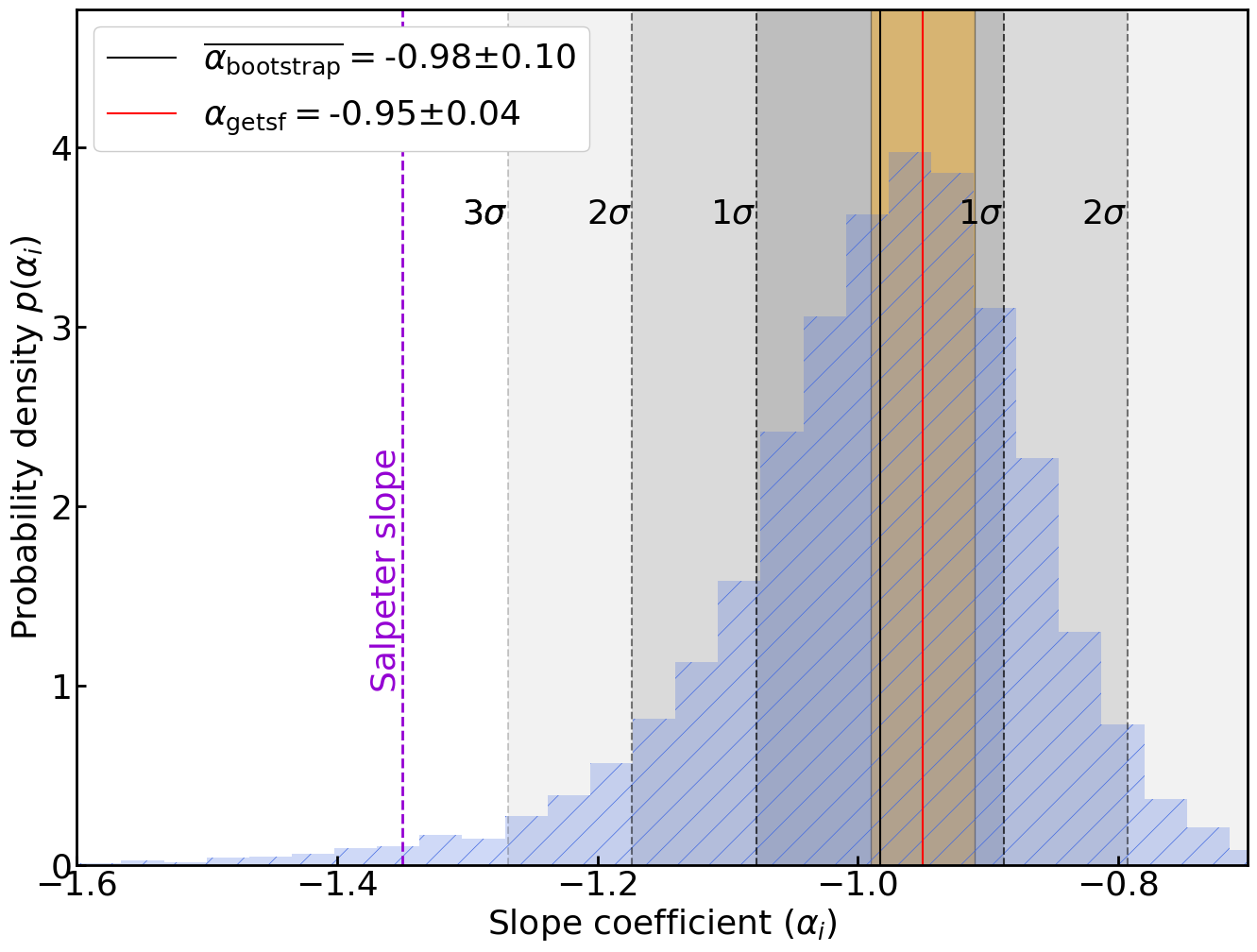
Figure 7: Bootstrapping probability density histogram of the $N=10^{4}$ slopes fitted using the Alstott et al. (2014) KS metric, measured for data sets generated using the metric parameters obtained for our sample of 205 cores. The black and red vertical lines indicate the resulting slope coefficient of $\alpha=-0.98\pm 0.10$ and the getsf fitted slope of $\alpha=-0.95\pm 0.04$ (orange area corresponding to 1$\sigma$, see Sect. 5.1). 1, 2, and 3$\sigma$ dispersions are estimated from the bootstrapping (shaded gray areas). The Salpeter slope (dashed vertical magenta line) is rejected with a probability of 99.98%.

We use statistical tests to compare the getsf CMF with either the GExt2D CMF or the Salpeter IMF. A two-sample Kolmogorov-Smirnov (KS) test is used to assess the likelihood that two distributions are drawn from the same parent sample (null hypothesis). In the case of the getsf and GExt2D CMFs, above the GExt2D completeness level we found no significant evidence that the core samples are drawn from different populations (with a KS statistic of $0.09$ and a p-value of $0.91$). We also used a statistical library based on the KS metric and dedicated to probability laws fitted by power-laws (Clauset et al. 2009; Alstott et al. 2014) to estimate the robustness of our linear regression fit. Run on the getsf CMF of W43-MM2&MM3 shown in Fig. 5a, this toolbox suggests that if fitted by a power-law, its best-fit parameters would be a slope coefficient of $\alpha=-0.95\pm 0.08$ above a minimum mass of $0.61\leavevmode\nobreak\ M_{\odot}$. This result is in good agreement with the regression fit performed on the getsf sample of cores, above our completeness level of $0.8\leavevmode\nobreak\ M_{\odot}$. Figure 7 presents the bootstrapping probability density histogram of the $N=10^{4}$ slopes fitted using the KS metric of Alstott et al. (2014), measured for data sets generated using the metric parameters obtained for our sample of 205 cores. The resulting slope coefficient is slightly steeper, $\alpha=-0.98\pm 0.1$, but still consistent with those found by the KS metric alone and the fitted value of Fig. 5a. Moreover, the sigma value obtained with this bootstrapping allows the Salpeter slope to be rejected with a probability of 99.98%, that is further than the $3.5\sigma$ level.

5.2 Robustness against our assumptions

Figure 6 shows various W43-MM2&MM3 ridge CMFs built for a different core catalog, under different assumptions of dust temperature and emissivity, and fit over a different mass range. For each CMF, we introduced randomly generated CMFs by varying core fluxes, dust temperatures, and opacities and computed the associated $3\,\sigma$ global uncertainty of their fit. We discuss below the robustness of the observed CMF slope against the chosen extraction strategy and assumptions behind the measurements of core masses.

Comparing Figs. 5a–b shows that the CMF of the W43-MM2&MM3 ridge is top-heavy regardless of the source extraction technique, either getsf or GExt2D (see Table 3). Of the 100 cores detected by both software packages (see Table 6), 90% have no significant differences in their integrated fluxes. Above the GExt2D completeness limit, they constitute the $1.1-69.9\leavevmode\nobreak\ M_{\odot}$ range of the CMF. This striking similarity argues for the robustness of core fluxes measured with different extraction methods, as long as they have a similar core definition.

Furthermore, when comparing Fig. 6a and Fig. 5a, our extraction strategy, which is based on bsens images denoised by MnGSeg, does not seem to impact quantitatively the W43-MM2&MM3 CMF. Figure 6a indeed presents the CMF of cores extracted in a companion paper (Paper V; Louvet et al. in prep.) from the original & cleanest images of the W43-MM2 and W43-MM3 protoclusters. In agreement with the noise level of the cleanest images at 1.3 mm (see Table 2), the 90% completeness limit of the cleanest core catalog is two times larger than that of the denoised & bsens CMF. The power-law index of the high-mass end of the original & cleanest CMF is close to, but even shallower than, that of the denoised & bsens CMF (see Table 4). The $\sim$75 cores detected in the cleanest image are in fact among the most massive cores listed in Table 7. Moreover, the consistency between the two CMFs comes from the fact that, on average, the original & cleanest cores have fluxes within 15% of their corresponding flux in Table 6 and are at worst within 50% of each other.

Beyond the uncertainty of flux measurements used to compute the core masses, the main uncertainties of CMFs arise from the mass-averaged dust temperature and dust opacity used to convert fluxes into masses (see Eq. B, Fig. 16, and Table 6). If we do not take into account the central heating by protostars and self-shielding of pre-stellar cores, the core temperatures would homogeneously be $\overline{T_{\rm dust}}\simeq 23\pm 2$ K. The CMF of getsf-extracted cores with a constant temperature (Fig. 6b) has a slightly shallower slope than when the individual dust temperature estimates are used (Fig. 5a, see Table 4). We also determined that the CMF flattening is robust against dust opacity variations. As the dust opacity is expected to increase with core density (e.g., Ossenkopf & Henning 1994), we made a test assuming a linear relation with mass, starting at $\kappa_{\rm 1.3mm}=0.007$ cm² g^-1 for the lowest-density core ($0.12\leavevmode\nobreak\ M_{\odot}$) and ending at $\kappa_{\rm 1.3mm}=0.015$ cm² g^-1 for the highest-density core ($69.9\leavevmode\nobreak\ M_{\odot}$). The resulting CMF has a power-law index lower than the CMF index found in Fig. 5a, but still greater than the Salpeter slope (see Fig. 6c and Table 4).

With all tests summarized in Tables 3 and 4, we can state that the W43-MM2&MM3 CMF is top-heavy with a power-law index within the $\alpha=[-1.02;-0.83]$ range. The resulting 1$\,\sigma$ uncertainty is estimated to be about $\pm 0.08$, still excluding the Salpeter slope.

6 Discussion on the origin of stellar masses

In Sect. 6.1, we compare the CMF of the W43-MM2&MM3 mini-starburst to published CMF studies. In the framework of several scenarios, we then predict the IMF that would result from the observed W43-MM2&MM3 CMF. In particular, we apply various mass conversion efficiencies (Sects. 6.1–6.2) and various subfragmentation scenarios (Sect. 6.3), and mention the other processes to consider (Sect. 6.4). Table 4 lists the parameters of the W43-MM2&MM3 IMFs derived and fitted under these various assumptions.

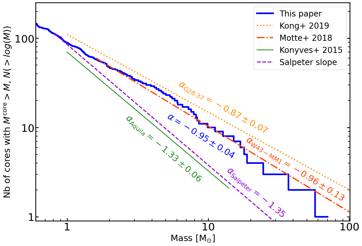
Figure 8: Comparison of the W43-MM2&MM3 CMF (blue histogram, see Fig. 5a) with power-laws fitted to the high-mass end, $>$1 $M_{\odot}$, of CMFs measured in three star-forming regions. The proto-typical CMF of low-mass star-forming regions, derived in Aquila (green line, Könyves et al. 2015), resembles the Salpeter slope of the canonical IMF (dashed magenta line, Salpeter 1955). In contrast, the CMFs in W43-MM2&MM3 and in the two high-mass star-forming protoclusters W43-MM1 and G28.37+0.07 (red dot-dashed and orange dotted lines, Motte et al. 2018b; Kong 2019) are top-heavy.

6.1 In the framework of the classical interpretation

CMFs measured in low-mass star-forming regions are generally strikingly similar to the IMF (e.g., Motte et al. 1998; Enoch et al. 2008; Könyves et al. 2015). In contrast, CMFs of Figs. 5a–b are much shallower than the high-mass end of the canonical IMF. The usual methodology to compare observed CMFs to the IMF is to assume a one-to-one correspondence between cores and stars and a given mass conversion efficiency of core mass into star mass. CMF studies of low-mass, low-density cores, $10^{5}-10^{7}$ cm^-3, often derived mass conversion efficiencies of $\epsilon_{\rm core}\sim 30-40\%$ (e.g., Alves et al. 2007; Könyves et al. 2015). We could expect a larger mass conversion efficiency for our extreme-density cores, $\gtrsim 5\times 10^{7}$ cm^-3 (see Table 7). Therefore, we assume here a mass conversion efficiency of $\epsilon_{\rm core}=50\%$, following Motte et al. (2018b). With this efficiency, the mass range of $0.8-69.9$ $M_{\odot}$, where the getsf sample is 90% complete, covers the progenitors of low- to high-mass stars, $0.4-35\leavevmode\nobreak\ M_{\odot}$. Fitting the CMF high-mass end, which would then formally start above $1\leavevmode\nobreak\ M_{\odot}$ or $2\leavevmode\nobreak\ M_{\odot}$, would lead to a slightly steeper slope, $\alpha$ values between $-0.98\pm 0.06$ and $-1.07\pm 0.07$, still shallower than the Salpeter slope of the canonical IMF (see Table 3 for a fit above $2\leavevmode\nobreak\ M_{\odot}$). As shown in Figs. 5a and 6d, the getsf CMFs for all cores and for those that should form low- to intermediate-mass stars are similarly flat (see Table 3). We refrain from fitting the CMF of high-mass cores alone because it has too few cores to be statistically robust. The flattening observed for the W43-MM2&MM3 CMF is a general trend in all mass regimes. Therefore, it cannot solely be attributed to high-mass stars that could form by processes different from those of low-mass stars (e.g., Motte et al. 2018a).

Figure 8 compares the high-mass end, $>$1 $M_{\odot}$, of the W43-MM2&MM3 CMF with a few reference CMF studies obtained in one low-mass star-forming region, Aquila (Könyves et al. 2015), and two high-mass protoclusters, W43-MM1 and G28.37+0.07 (Motte et al. 2018b; Kong 2019). All published studies of core populations found in the nearby, low-mass star-forming regions have argued for the interpretation that the shape of the IMF can simply be derived directly from the CMF (e.g., Motte et al. 1998; André et al. 2014). We here use a similar definition for cores and very similar tools to extract them to those used in these studies. In particular, getsf (Men’shchikov 2021) has the same philosophy as the software used to extract cores from Herschel images, getsources and CuTEx (Men’shchikov et al. 2012; Molinari et al. 2011), and ground-based images, MRE-GCL (Motte et al. 2007). Even so, the CMF measured for the W43-MM2&MM3 ridge is different from the CMF found in low-mass star-forming regions, including Aquila, which was studied in detail with Herschel (Könyves et al. 2015, see Fig. 8). It has a high-mass end shallower than most published CMFs, and thus shallower than the IMF of Salpeter (1955). It only resembles, for now, the CMFs observed for the W43-MM1 mini-starburst ridge (Motte et al. 2018b) and the G28.37+0.07 filament (Kong 2019) (see Fig. 8).

The CMF results obtained for both the W43-MM2&MM3 and W43-MM1 ridges indicate that either their IMF will be abnormally top-heavy and/or that the mapping between their core and star masses will not be direct. In the framework of the first interpretation, we assume that the shape of the IMF is directly inherited from the CMF. The results from these two mini-starbursts would thus put into question the IMF universality, which is now being debated (e.g., Hopkins 2018). In the framework of the second interpretation, several processes could, in principle, help reconcile the top-heavy CMF observed in the W43-MM2&MM3 ridge with a Salpeter-like IMF. We investigate below the effect of several of them: mass conversion efficiency, core subfragmentation, star formation history, and disk fragmentation.

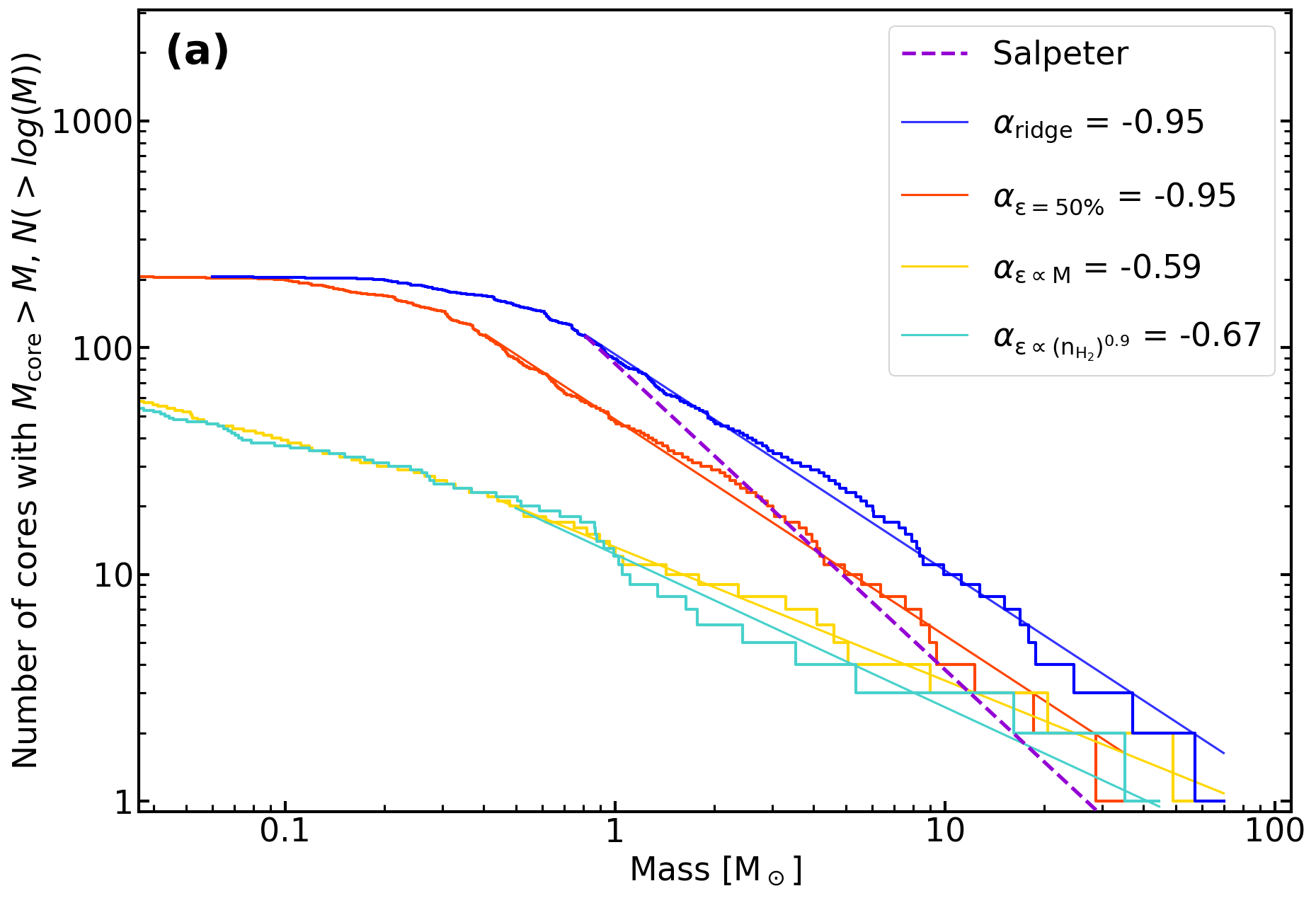
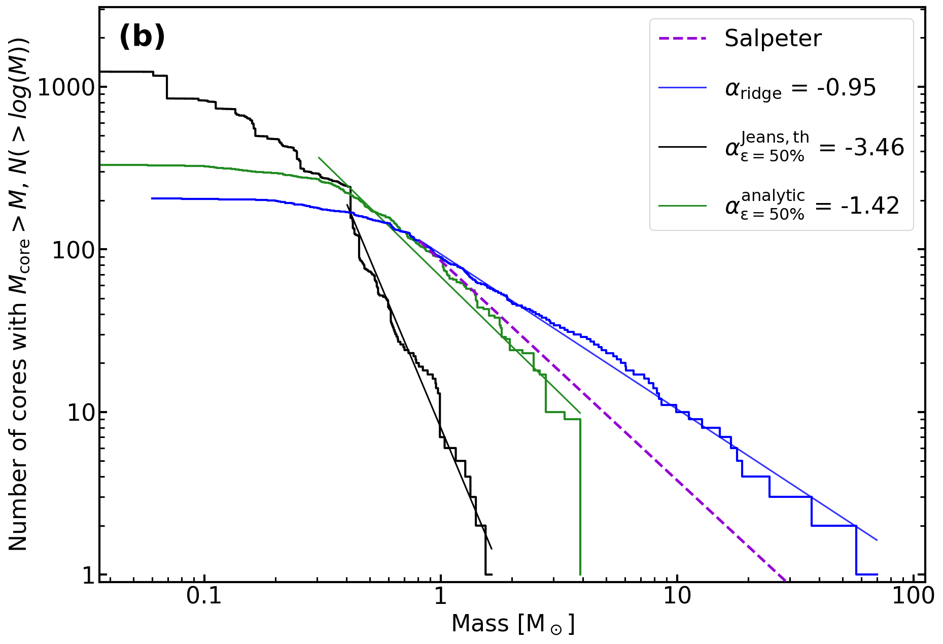
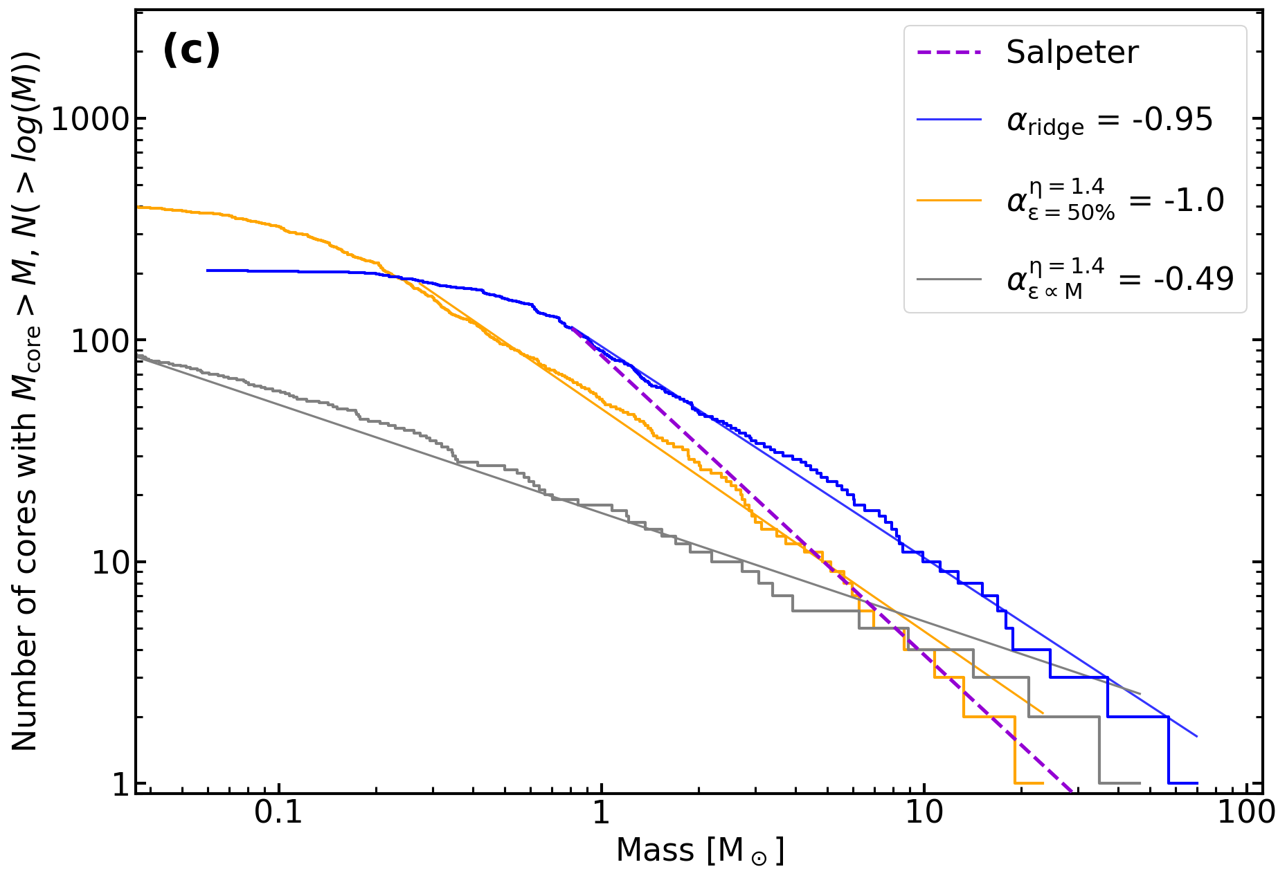
Figure 9: IMFs resulting from various mass conversion efficiencies and fragmentation scenarios, all applied to the W43-MM2&MM3 CMF of Fig. 5a (blue histogram). Panel (a): IMFs predicted for a constant mass conversion efficiency of 50% (red histogram), linear with the mass (yellow histogram), and dependent on the core density (Louvet et al. 2014, cyan histogram) (see Sect. 6.2). Panel (b): IMFs predicted by the two extreme fragmentation scenarios in Sect. 6.3: thermally supported Jeans fragmentation (black) and the analytic fragmentation function leading to a Salpeter slope (green histogram). Panel (c): IMFs predicted by the hierarchical cascade scenario of Thomasson et al. (subm.), leading to binary fragments. A 2:1 mass partition and two constant mass conversion efficiencies, 50% (orange histogram) or linear with the mass (gray histogram), are assumed. The number of fragments is taken as the lower integer, with a minimum of 1.

6.2 Using different mass conversion efficiencies

In the present paper we define cores as emission peaks whose sizes are limited by their structured background and neighboring cores. In dynamical clouds, however, the mass, the structure, and even the existence of these cores will evolve over time, as they are expected to accrete or dissolve gas from their background and split into several components or merge with their neighbors (e.g., Smith 2014; Motte et al. 2018a; Vázquez-Semadeni et al. 2019). To account for both these static and dynamical views of cores, we used different functions for the conversion efficiency of core mass into star mass and predict the resulting IMF.

We first assume a mass conversion efficiency that accounts for the mass loss associated with protostellar outflows in the core-collapse model (Matzner & McKee 2000). With a constant mass conversion efficiency with core mass, the IMF has the same shape as the CMF as it is simply shifted to lower masses. As mentioned in Sect. 6.1, we choose a mass conversion efficiency of $\epsilon_{\rm core}=50\%$. Figure 9a displays the IMF resulting from cores whose distribution is shown in Fig. 5a. The predicted IMF presents, as expected, the same high-mass end slope above $\sim$0.4$\leavevmode\nobreak\ M_{\odot}$ (see Table 4).

In the case of dynamical clouds, the competitive or gravitationally driven accretion process allows high-mass cores to more efficiently accrete gas mass from their surroundings than low-mass cores (e.g., Bonnell & Bate 2006; Clark & Whitworth 2021). This generally leads to efficiencies of the core formation and mass conversion that depend, to the first order, on the clump and core masses, respectively. We use two analytical models for the mass conversion efficiency.

Since the gravitational force scales linearly with mass, as a first toy model we assumed a linear relation between the mass conversion efficiency and the core mass, normalized by its maximum value: $\epsilon_{\rm core}=\frac{M}{69.9\,M_{\odot}}\times 100\%$. The IMF resulting from this relation applied to the CMF of Fig. 5a presents a much shallower high-mass end slope (see Fig. 9a and Table 4).

As a second toy model, we assumed a mass conversion efficiency depending on the mean volume density of cores, normalized by its maximum value: $\epsilon_{\rm core}=\left(\frac{n_{\rm{H_{2}}}}{2.2\times 10^{8}{\rm cm}^{-3}}\right)^{0.9}\times 100\%$. This quasi-linear relation is an extrapolation at 3 400 au scales (the typical size of our cores) of the relation observed in W43-MM1 for large cloud structures, $\sim$1 pc (Louvet et al. 2014). The IMF resulting from this toy model has a high-mass end slope which is slightly shallower than the CMF of Fig. 5a (see Fig. 9a and Table 4).

Therefore, the fact that a core is no longer considered a static and isolated cloud structure, but rather a cloud structure that accretes its mass from its surrounding cloud at a rate depending on its mass and location in the cloud, tends to flatten the high-mass end of the predicted IMF relative to the observed CMF of cores. This result is in qualitative agreement with analytical models following the evolution of the CMF through the growth of core mass expected in dynamical clouds (Dib et al. 2007; Hatchell & Fuller 2008; Clark & Whitworth 2021).

6.3 Using different scenarios of core subfragmentation

The definition of a core is also closely associated with the angular resolution of the observed (or simulated) images of a protocluster (see Lee & Hennebelle 2018; Pelkonen et al. 2021; Louvet et al. 2021). The turbulent subfragmentation within these core entities cannot be neglected, but fragmentation functions are barely constrained. We therefore assumed three extreme fragmentation scenarios after applying a 50% mass conversion efficiency to the W43-MM2&MM3 CMF displayed in Fig. 5a. Figure 9b presents the resulting distribution of fragment masses, here called core fragmentation mass function, as in Elmegreen (2011), and sometimes also called system mass function (Clark & Whitworth 2021). Since a mass conversion efficiency is applied beforehand, the core fragmentation mass function could directly correspond to the IMF.

The first most extreme fragmentation scenario is the Jeans fragmentation of a core only supported by its thermal pressure. Under this hypothesis and with a mass conversion efficiency of $\epsilon_{\rm core}=50\%$, we assume a mass equipartition between fragments; the number of fragments is thus half the ratio of the core mass to its Jeans mass, $N_{\rm frag}(M)=0.5\times\frac{M}{M_{\rm Jeans}}$. We took the measured temperature and FWHM size of our cores (see Tables 6-7) and computed the Jeans mass of fragments within cores with masses ranging from $2\leavevmode\nobreak\ M_{\odot}$ and $\sim$70$\leavevmode\nobreak\ M_{\odot}$. In the W43-MM2&MM3 ridge, most cores are super-Jeans and the most massive cores, in the $16-70\leavevmode\nobreak\ M_{\odot}$ range, would fragment into $50-85$ objects. The resulting IMF is much steeper than the CMF of Fig. 5a and even steeper than the Salpeter slope of the canonical IMF (see Fig. 9b and Table 4).

As a second extreme scenario, we found that a fragmentation function of the form $N_{\rm frag}(M)=\left(\frac{\epsilon_{\rm core}\times M}{0.12\;M_{\odot}}\right)^{0.4}$ is necessary to steepen the high-mass end slope of the CMF to a core fragmentation mass function and IMF with a slope close to Salpeter (see Fig. 9b). This analytical function predicts a single star in $0.24\leavevmode\nobreak\ M_{\odot}$ cores, about five stars in $16\leavevmode\nobreak\ M_{\odot}$ cores and about ten stars in the $\sim$70 $M_{\odot}$ core of W43-MM2. These fragmentation prescriptions may apply to evolved cores (referred to as IR-bright), which are observed with a high level of fragmentation (Brogan et al. 2016; Palau et al. 2018; Tang et al. 2021). However, most of the W43-MM2&MM3 cores are expected to be much younger (Motte et al. 2003). Since the subfragmentation of young cores (referred to as IR-quiet or IR-dark) is rarely observed and therefore very poorly constrained, we simply assume similar levels of fragmentation from young massive clumps to cores, that is from $\sim$20 000 au to $\sim$2 000 au scales, and from cores to fragments, that is from $\sim$2 000 au to $\sim$500 au scales. If we follow studies by Bontemps et al. (2010), Palau et al. (2013), Busquet et al. (2016) and Louvet et al. (2019) showing that high-mass clumps generally fragment in two cores at most, the two extreme fragmentation scenarios proposed above are both unlikely to be taking place in the W43-MM2&MM3 ridge.

A third fragmentation scenario is derived from a new type of model aimed at constraining the hierarchical cascade, also called the fragmentation cascade, in observed and simulated clouds (e.g., Thomasson et al. subm.). These studies are based on the finding that the density structure of molecular clouds is hierarchical, and more precisely multi-fractal (Elmegreen et al. 2001; Robitaille et al. 2020), and that the spatial distribution of stars is also hierarchical (Joncour et al. 2017, 2018). Thomasson et al. (subm.) studied the fractal hierarchical cascade of the intermediate-mass star-forming region NGC 2264, using Herschel-based column density maps. The authors found, for clustered clumps, a fractal fragmentation index of $\eta\simeq 1.4\pm 0.1$, from the clump to the core scales and more precisely from 13 000 au to 5 000 au. A fractal index of $\eta=1.4$ means that for every factor of $2$ decrease in physical scale, the number of fragments multiplies by $1.4$. If we use this fractal index to extrapolate to scales ranging from 2 500 au to 500 au and generally apply it to all of our cores, we expect to find about two fragments at 500 au resolution within our $0.12-69.9\leavevmode\nobreak\ M_{\odot}$ cores. Below this 500 au scale, we assume that disk fragmentation dominates turbulent fragmentation and that therefore the hierarchical cascade stops. The distribution of the core mass between subfragments, hereafter called mass partition, is not yet well constrained; we assume below two different cases.

The simplest case assumes a uniformly random mass distribution. As shown by Swift & Williams (2008), among others, with this mass partition the high-mass end slopes of the core fragmentation mass function of fragments and the resulting IMF cannot change much from that of the CMF of their parental cores.

For the second case we can assume a very unbalanced mass partition. A preliminary study of 11 W43-MM2&MM3 core systems identified within $<\,2\,\Theta_{\rm beam}$ distances (or 5000 au in Fig. 1a) suggests mass partition fractions close to 2:1. Interestingly, this is consistent with observations of other high-mass core systems (Busquet et al. 2016; Motte et al. 2018b). Such an unbalanced mass partition is also predicted in the competitive accretion model of Clark & Whitworth (2021), which shows that the large majority of the core mass is used to increase the masses of existing fragments. This unbalanced mass partition and a mass conversion efficiency of $\epsilon_{\rm core}=50\%$, applied to the W43-MM2&MM3 CMF, slightly steepens the high-mass end slope (see Fig. 9c and Table 4).

As the last and most complex test, we assumed the third fragmentation scenario with a 2:1 mass partition and a mass conversion efficiency depending on the core mass, $\epsilon_{\rm core}\propto M$. The resulting IMF is top-heavy with a slope even shallower than that in Fig. 5a. Interestingly, these assumptions tend to agree with the model of Clark & Whitworth (2021), which combines turbulent fragmentation and competitive accretion. The high-mass end of the the predicted core fragmentation mass functions is broadly invariant over time because the formation of new multiple cores balances the accretion of the gas mass onto existing cores.

6.4 In the framework of other processes

Beyond the turbulent fragmentation discussed in Sect. 6.3, disk fragmentation and N-body interactions could further alter the shape of the core fragmentation mass function and thus of the resulting IMF of single stars. Stellar multiplicity studies of low- to intermediate-mass systems have generally revealed mass equipartition (Duquennoy & Mayor 1991), which would not impact the slope of the IMF high-mass end (e.g., Swift & Williams 2008). In contrast, given the low number statistics of high-mass star studies, the mass partition of stellar systems that contain high-mass stars is poorly constrained (Duchêne & Kraus 2013). Because of the lack of constraints on disk fragmentation and on N-body interactions, we did not apply a model to the core fragmentation mass function to determine the IMF of single stars.

The other process used to reconcile the observed top-heavy CMF high-mass end with a Salpeter-like CMF is the continuous formation of low-mass cores versus short bursts of formation of high-mass stars. In the case of dense clumps or ridges, most high-mass cores could indeed form in short bursts of $\sim$10⁵ years, while lower-mass cores would more continuously form over longer periods of time. We recall that the IMF of young stellar clusters of a few $10^{6}$ years is the sum of several instantaneous CMFs built over one to two free-fall times with $\tau_{\rm free-fall}\simeq 10^{5}$ years. Before and after a burst with a single top-heavy CMF, about ten star formation events of more typical CMFs could develop, diluting the top-heavy IMF resulting from the star formation burst into an IMF with a close-to-canonical shape. Studying the evolution of the CMF shape over time is necessary to quantify this effect, and is one of the goals of the ALMA-IMF survey (see Paper I and Paper V; Motte et al. 2021, Louvet et al. in prep.).

In conclusion, it is difficult to predict the resulting IMF from the observed CMF in the W43-MM2&MM3 ridge. However, the various mass conversion efficiencies and fragmentation scenarios discussed here suggest that the high-mass end of the IMF could remain top-heavy. This will have to go through the sieve of more robust functions of the mass conversion efficiency and core subfragmentation, and of better constrained disk fragmentation and burst-versus-continuous star formation scenarios. If it is confirmed that the predicted IMF of W43-MM2&MM3 is top-heavy, this result will clearly challenge the IMF universality. If we dare to generalize, the IMFs emerging from starburst events could inherit their shape from that of their parental CMFs and could all be top-heavy, disproving the IMF universality.

7 Summary and conclusion

We used ALMA images of the W43-MM2&MM3 mini-starburst to make an extensive census of cores and derive its CMF. Our main results and conclusions can be summarized as follows:

• We combined the 12 m array images of the W43-MM2 and W43-MM3 protoclusters that were individually targeted by the ALMA-IMF Large Program (see Sect. 2 and Table 1; Motte et al. 2021; Ginsburg et al. 2021). At 1.3 mm, the resulting $\rm 4.2\leavevmode\nobreak\ pc\times 3.2\leavevmode\nobreak\ pc$ mosaic has a spatial resolution of $\sim$0.46″, or 2 500 au. The 3 mm mosaic is wider, $\rm 7.3\leavevmode\nobreak\ pc\times 5.3\leavevmode\nobreak\ pc$, with a similar angular resolution but a mass sensitivity about three times lower (see Fig. 14).

• To have the most complete and most robust sample of cores possible, we used both the best-sensitivity and the line-free ALMA-IMF images and removed part of the cirrus noise with MnGSeg (see Sect. 3). This new strategy proved to be efficient both in increasing the number of sources detected and in improving the accuracy of their measurements, when applied to present observations and synthetic images (see Table 2 and Appendix A). In the end, it allows the $5\,\sigma$ detection of point-like cores with gas masses of $\sim$0.20 $M_{\odot}$ at 23 K (see Fig. 1a).

• We extracted 1.3 mm compact sources using both the getsf and GExt2D software packages. getsf provides a catalog of 208 objects, which have a median FWHM size of 3 400 au (see Table 6 and Figs. 1–2). The 100 cores extracted by both getsf and GExt2D have sizes and thus fluxes, on average, consistent to within 30%.

• The nature of the W43-MM2&MM3 sources is investigated to exclude free-free emission peaks and correct source fluxes from line contamination (see Figs. 3–4 and Sects. 4.1.1–4.1.2). The resulting catalog contains 205 getsf cores (see Table 7). Their masses are estimated and, for the most massive cores, they are corrected for their optically thick thermal dust emission (see Eq. 6 in Sect. 4.2 and Appendix B). The core mass range is $0.1-70\leavevmode\nobreak\ M_{\odot}$ and the getsf catalog is 90% complete down to $0.8\leavevmode\nobreak\ M_{\odot}$ (see Appendix C).

• The W43-MM2&MM3 CMFs derived from the getsf and GExt2D core samples are both top-heavy with respect to the Salpeter slope of the canonical IMF (see Sect. 5.1 and Fig. 5). The high-mass end of the getsf CMF is well fitted, above its 90% completeness limit, by a power-law of the form $N(>\log M)\propto M^{\alpha}$, with $\alpha=-0.95\pm 0.04$ (see Table 3). The error bars include the effect of uncertainties on core mass, fit, and completeness level. The CMF high-mass end thus cannot be represented by a function resembling the Salpeter IMF (see also Fig. 7). We showed that the shape of the CMF is robust against flux differences arising from the map or software chosen to extract cores, and against variations of the dust emissivity and temperature variations (see Sect. 5.2, Fig. 6 and Table 4). Our result, in striking contrast with most CMF studies, argues against the universality of the CMF shape.

• We used different functions of the conversion efficiency from core to stellar masses to predict the IMF resulting from the W43-MM2&MM3 CMF (see Sect. 6). While in the framework of the core-collapse model the slope of the IMF high-mass end remains unchanged, it becomes shallower for competitive accretion or hierarchical global collapse models (see Fig. 9a). We explored several fragmentation scenarios, which all slightly steepen the high-mass end of the predicted IMF (see Fig. 9b–c). It is possible to set an artificial analytical model that predicts an IMF with the Salpeter slope. However, the best-constrained fragmentation model, which is a hierarchical cascade with 2:1 mass partition, predicts an IMF slope which does not reconcile with the canonical value (see Fig. 9c). Most scenarios tested here suggest that the resulting IMF could remain top-heavy. More constrained functions of the mass conversion efficiency, core subfragmentation, disk fragmentation, and burst development are required to provide a more definitive prediction. However, if this result is confirmed, the IMFs emerging from starburst events could inherit their shape from that of their parental CMFs and be top-heavy, thus challenging the IMF universality.

Appendix A Quality of the core extraction carried out using images denoised by MnGSeg

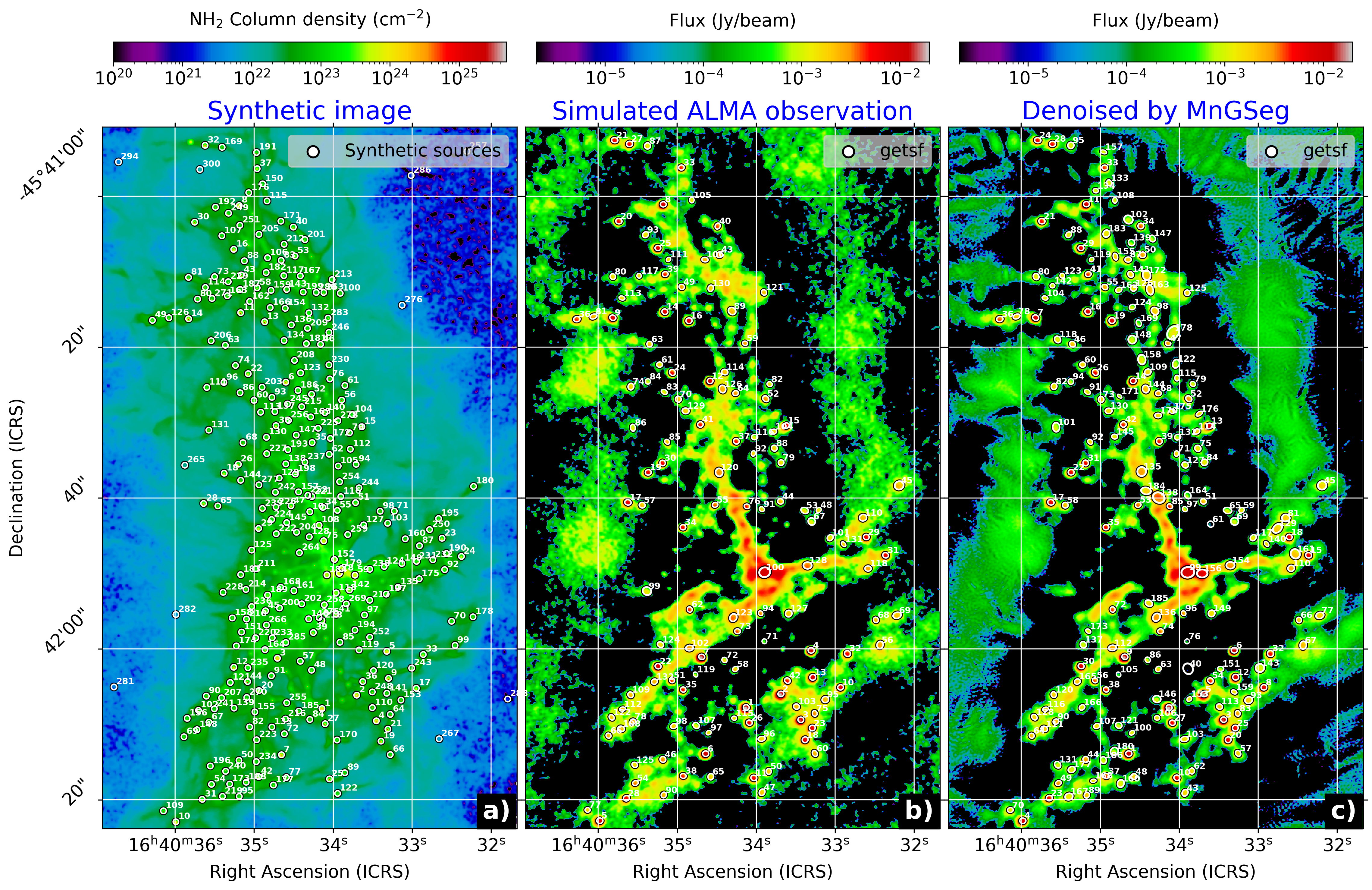
Figure 10: Synthetic column density images used to qualify the extraction of cores in images denoised by MnGSeg. Panel a): Projected column density map of a numerical simulation by Ntormousi & Hennebelle (2019), from which simulated cores have been removed and to which synthetic sources have been added ($0.2-3.2\leavevmode\nobreak\ M_{\odot}$ cores with a $I(\theta)\propto\theta^{-1}$ intensity profile up to $0.5\arcsec$). Panel b): Simulation of the ALMA imaging of the column density map of a at 1.3 mm, with a 240-minutes integration time and a beam size of $0.81\arcsec\times 0.76\arcsec$. Panel c): Simulated ALMA image from b), with noise reduced by $\sim$30% using MnGSeg. Cores are outlined by ellipses and labeled by numbers according to the truth table (in a)) and getsf identifiers in the original and denoised catalogs (in b) and c)).

Core extractions are limited by the noise level of input images. The noise measured in any molecular cloud image can schematically be seen as the sum of the white instrumental noise at scales smaller than the beam, interferometric artifacts (when applicable), and some structural noise. MnGSeg is an efficient technique to separate the hierarchical cloud structures into coherent structures associated with star formation and incoherent Gaussian structures (Robitaille et al. 2019). The latter consist of structures that do not persist from scale to scale including white noise and low-density cirrus clouds on the line of sight to our star formation sites. We used MnGSeg to remove Gaussian structures of our image at scales larger than the beam, thus removing structural noise like our low-density cirrus. In practice, we keep coherent structures, point-like structures that correspond in particular to isolated cores, interferometric artifacts, and the white instrumental noise, which is a flux component needed to reliably extract cores. We hereafter call this image the denoised image since the noise level decreases (see Table 1).

To characterize the quality of the core extraction performed on images denoised by MnGSeg, it is necessary to quantify the gain of the catalog in terms of number of detected cores, fraction of spurious sources, and quality of the flux measurements. To do so, we studied core extractions done on a synthetic image, consisting of a background image plus well-characterized synthetic sources. For the background image, we used a column density image created by Louvet et al. (2021) from a three-dimensional numerical simulation of an Orion-sized turbulent molecular cloud (Ntormousi & Hennebelle 2019). For our purpose, we assumed it represents a typical cloud complex of the ALMA-IMF Large Program like G338.93, located at 3.9 kpc. The simulated density cube was projected along a single axis and a core extraction was performed with getsf to remove the flux contribution of simulated cores, thus creating an image only made of their background. These cores are not suitable for our purpose due to their ill-constrained sizes and masses. A total of 306 synthetic sources were then added where the column density exceeds $4\times 10^{22}\leavevmode\nobreak\ \textrm{cm}^{-2}$. They have masses arranged in ten logarithmic bins spanning $0.2-3.2\leavevmode\nobreak\ M_{\odot}$ and, for simplicity, they are set to be unresolved by the simulated ALMA beam (here $0.8\arcsec$). The resulting column density image is presented in Fig. 10a. All the characteristics of synthetic sources are stored in a reference table hereafter called the truth table.

Afterward, we simulated the ALMA observation of this synthetic protocluster using the CASA task simobserve (see Fig. 10b). We first created an image of the 1.3 mm, or more precisely 224.55 GHz, flux arising from the synthetic column density image of Fig. 10a, assuming a dust temperature of 20 K and a dust $+$ gas mass opacity of $\kappa_{\rm 1.3mm}=\rm 0.01\leavevmode\nobreak\ cm^{2}\,g^{-1}$. By specifying a typical array configuration of ALMA-IMF images and a given integration time, simobserve uses an incomplete UV coverage to smooth the synthetic image to a $0.81\arcsec\times 0.76\arcsec$ beam and creates interferometric artifacts, including filtering of the extended emission. It then adds some white noise, which is characteristic of submillimeter observations. Finally, we applied MnGSeg to this original image and removed all incoherent structures with sizes larger than the beam (see definition above and Fig. 10c).

[c] Extraction strategy Cores Cores (number and their proportion in the getsf catalog) Detection Measurement extracted correctly with bad with rough with bad with rough by getsf extracted detection measurement (1) (2) (3) (4) (5) (6) (7) (8) original original 132 128 (97%) 0 1 (1%) 4 (3%) 21 (16%) denoised original 183 163 (90%) 0 5 (3%) 18 (10%) 27 (15%) denoised denoised 183 173 (95%) 0 6 (3%) 10 (5%) 32 (17%)

Table 5: Quality of core extractions done using the original and denoised images of Fig. 10b-c for either detection or measurement or both.

• (4) Extracted cores, whose peak position is at worst partly inaccurate, and whose flux measurement is inaccurate by at worst a factor of 2 (see definitions below).

• (5) Detected cores, whose peak position is very inaccurate: $\Theta_{\textrm{offset-position}}>\Theta_{\textrm{beam}}/2$.

• (6) Detected cores whose peak position is partly inaccurate: $\Theta_{\textrm{beam}}/4<\Theta_{\textrm{offset-position}}\leq\Theta_{\textrm{beam}}/2$.

• (7) Correctly extracted cores, whose flux measurement is inaccurate by at least a factor of 2, $\frac{S^{\rm int}_{\rm measured}}{S^{\rm int}_{\rm true}}<\frac{1}{2}$ or $>2$. These sources are not considered correctly extracted cores (see Col. 4), and as such are excluded when estimating completeness levels in Fig. 13.

• (8) Correctly extracted cores, whose flux measurement is inaccurate by a factor between 1.5 and 2, $\frac{1}{2}\leq\frac{S^{\rm int}_{\rm measured}}{S^{\rm int}_{\rm true}}<\frac{2}{3}$ or $\frac{3}{2}<\frac{S^{\rm int}_{\rm measured}}{S^{\rm int}_{\rm true}}\leq 2$. Roughly detected cores generally have rough measurements.

We compared the core extractions done by getsf (Men’shchikov 2021) on the original and denoised images of Figs. 10b-c. We applied the post-selection criteria recommended by getsf and described in Sect. 3 to remove sources that are not reliable enough. Table 5 lists the number of cores, detected by getsf, which correspond to real synthetic cores. Since the noise level is $\sim$30% smaller in the denoised image (see Table 1), getsf detected an increased number of sources, $40\%$ more than in the original image (see Table 5).

Table 5 also quantifies the quality of core extractions, from their detection to their flux measurement. To identify the “correctly detected” cores, we cross-matched the getsf catalogs and the truth table. Their peak positions are considered accurate when they lie at less than $\Theta_{\textrm{beam}}/2\simeq 0.4\arcsec$ from the position of a synthetic core in the truth table. A “badly detected” source refers to a source whose peak position is inaccurate by more than this value, and consequently not present in the synthetic core population. The getsf software was adjusted by Men’shchikov (2021) not to return any badly detected sources, also called spurious source. All cores identified in both in the original and denoised images of Figs. 10b-c qualify as correctly detected, without spurious detections. To go beyond this binary description of core detection, Table 5 lists the number of “roughly detected” cores, which are those with peak position offset by more than $\Theta_{\textrm{beam}}/4\simeq 0.2\arcsec$, but less than $\Theta_{\textrm{beam}}/2\simeq 0.4\arcsec$. These cores consist of the merging of a synthetic core and part of its surrounding background cloud, which inevitably has consequences on the flux measurement, as shown below. The number of roughly detected cores barely increased, from 1% to 3%, when applying the MnGSeg technique to denoise the simulated ALMA image (see Table 5).

We investigated the quality of the flux measurements of cores extracted both in the original and denoised images by computing the ratios of the getsf integrated fluxes over the true fluxes. Given the complexity of the process of extracting cores in molecular clouds, we qualify a core as correctly extracted when its flux measurement is correct within a factor of 2, $\frac{1}{2}\leq\frac{S^{\rm int}_{\rm measured}}{S^{\rm int}_{\rm true}}\leq 2$. An inaccuracy of the flux ratio larger than 2 indicates a source with a “badly measured” flux, while a flux ratio between 1.5 and 2 indicates it is “roughly measured”. Table 5 shows that measurements in the denoised image are as accurate as those made in the original image. When cores are detected in the denoised image and their flux measured in the noisier original image, the latter are less accurate but not by large factors. Figures 11a-c, display the ratios of the getsf fluxes over the true fluxes for the different detection and measurement images. Undetected sources of a given bin mass lie in the hatched regions of Figs. 11a–c, leading to non-continuous source groups. For cores down to the $0.28\leavevmode\nobreak\ M_{\odot}$ bin, which is below the 90% completion level of $0.37\leavevmode\nobreak\ M_{\odot}$ (see Fig. 12), median fluxes are correct by $\sim$10% for the three extraction runs. The additional sources of the denoised catalog (out of the hatched region of Fig. 11c, contrary to Fig. 11a), whose detection and flux measurement were estimated as not reliable enough in the original image, have less accurate fluxes, but for 90% of them they remain correct to within a factor of 2 and on average are better than a factor of 1.55.

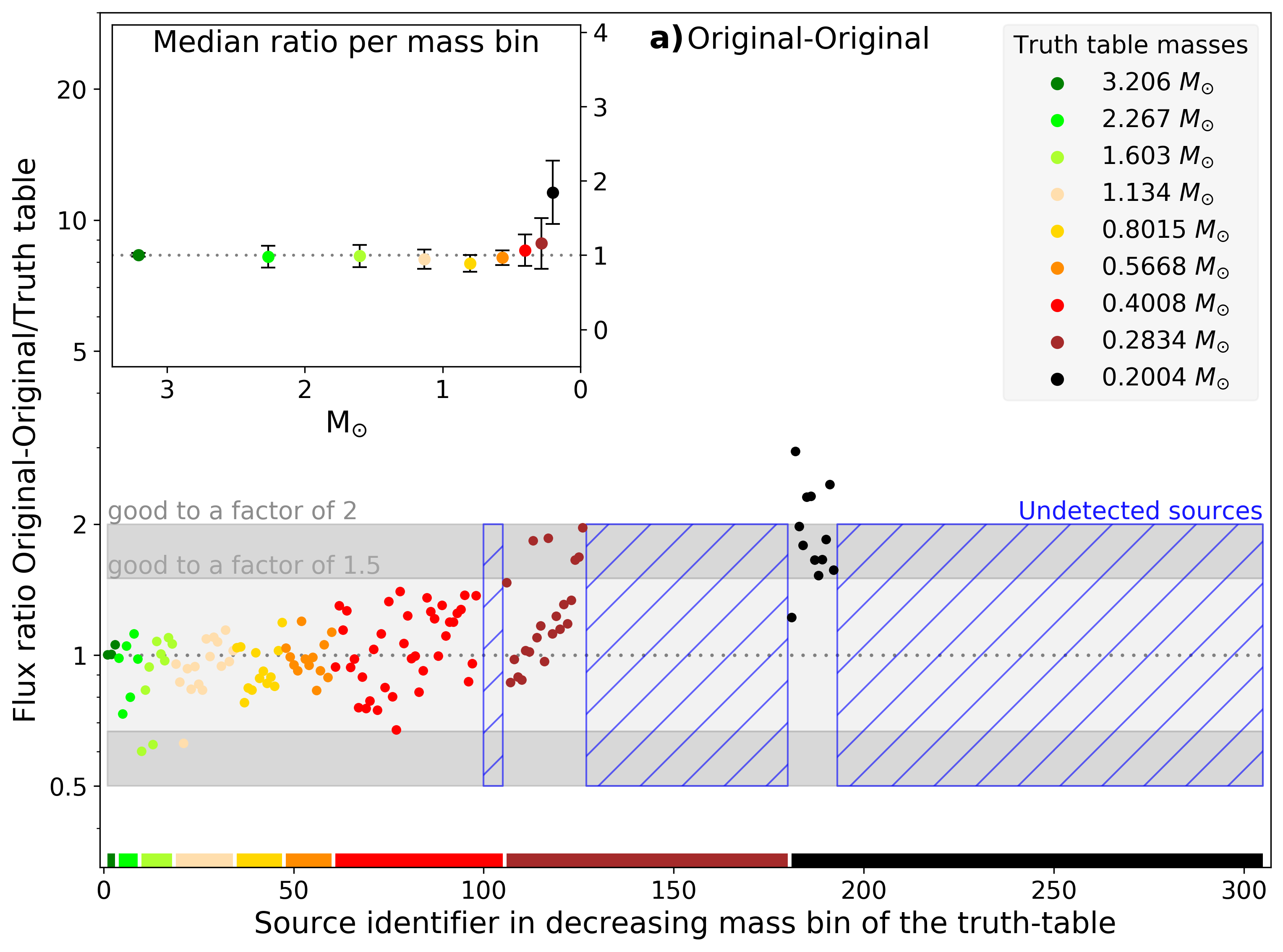
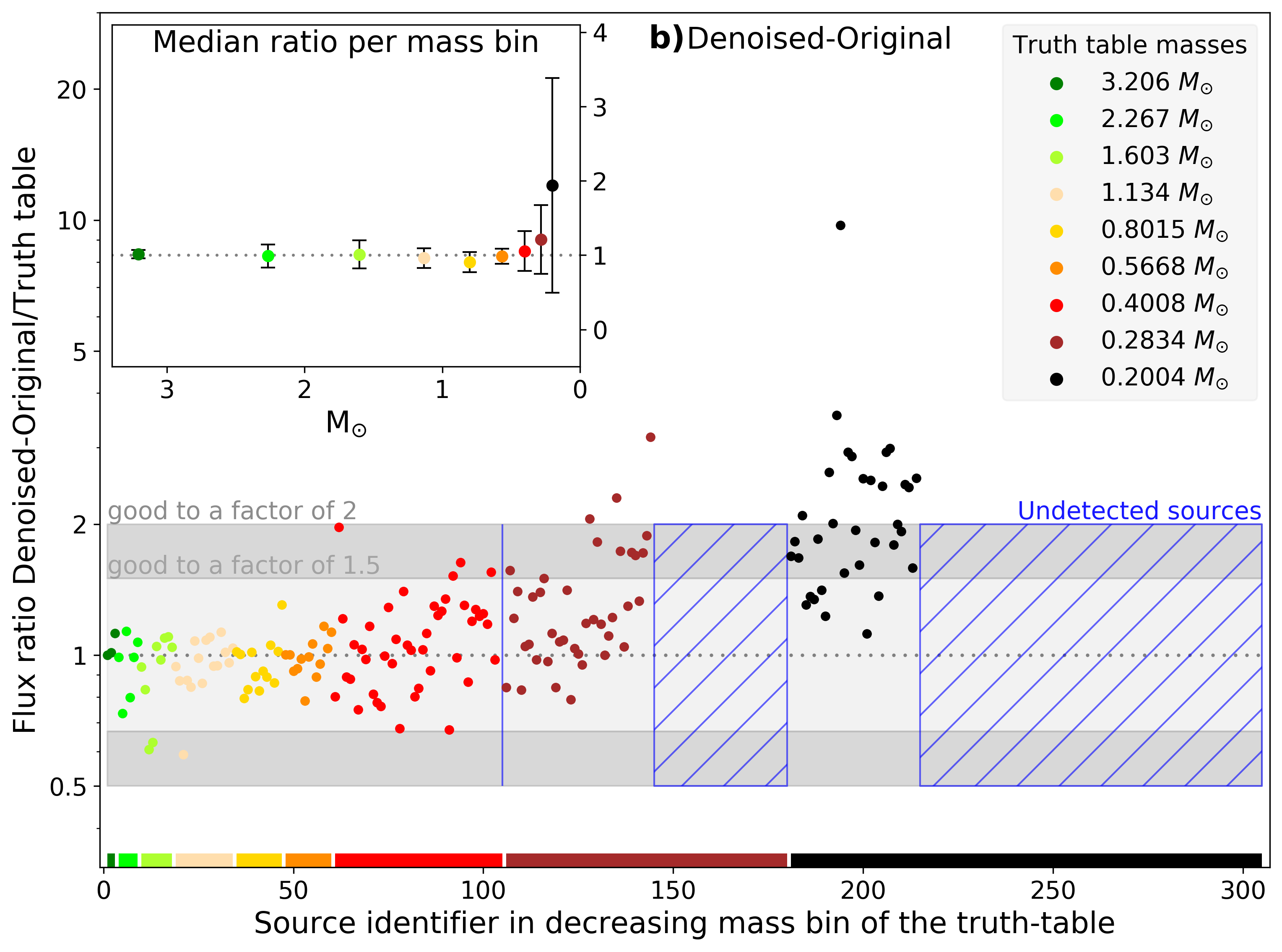
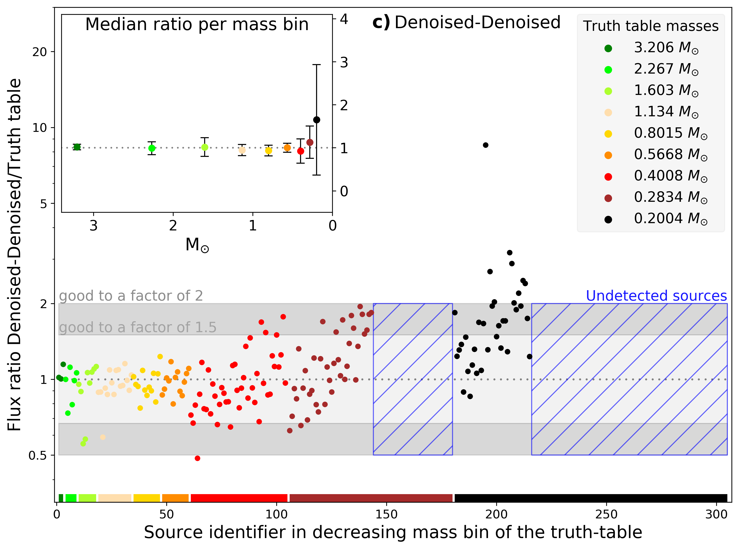
Figure 11: Quality of the flux measurements made by getsf when sources are both detected and extracted in the original image (in a), detected in the denoised and measured in the original images (in b), and both detected and measured in the denoised image (in c). The ratios of the getsf integrated fluxes to the true fluxes are plotted for individual sources, arranged in decreasing mass bin (main panel) and median values for the nine mass bins (enclosed plots). Blue hatched regions represent fraction of the truth table sources undetected by the algorithm, for each mass bin. For cores down to the $0.28\leavevmode\nobreak\ M_{\odot}$ bin, fluxes are correct by $\sim$10% for the three extraction runs. The denoised image provides a catalog with 40% more sources whose flux measurements are, for 90% of them, better than a factor of 2.

These synthetic simulations strongly suggest that denoising real images with MnGSeg provide the opportunity to extract a larger number of cores with good flux measurements. The parameters of the sources, such as sizes and fluxes, appear more accurate when measured directly in the denoised image (see enclosed plots of Fig. 11). Completeness levels of the denoised versus original core extractions can also be measured to quantify the gain when denoising the simulated ALMA image using MnGSeg. Figure 12 shows that the 90% completeness level improved by $\sim$16%. While this value depends on the chosen background and core shape, such an improvement of the completeness level is a definite asset for studies of the mass and spatial distributions of cores. We therefore expect that the denoising process proposed by MnGSeg will improve the statistics of core catalogs and their resulting studies.

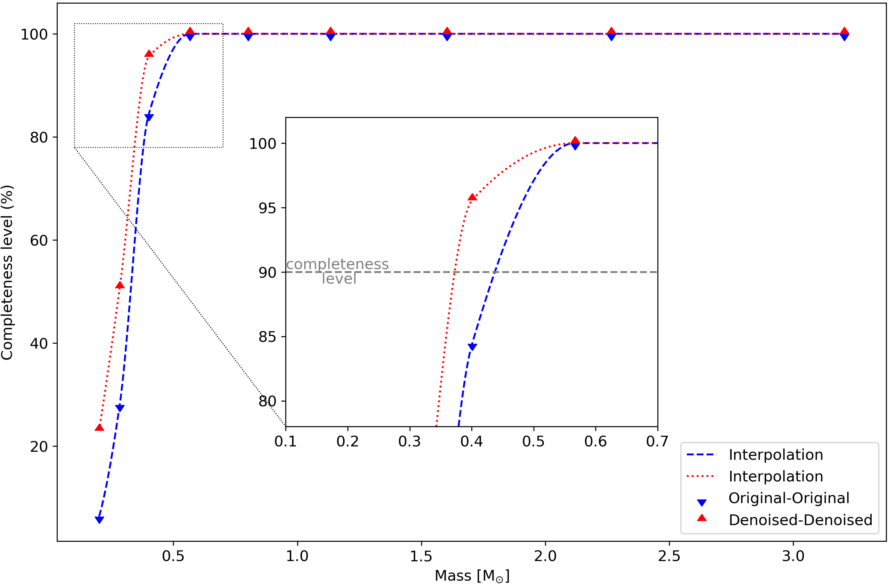
Figure 12: Completeness levels of the core samples of the original and denoised catalogs obtained by getsf, excluding badly detected and badly measured sources. Data points were interpolated using the Piecewise Cubic Hermite Interpolating Polynomial method. The core content is 90% complete down to $\sim$$0.44\leavevmode\nobreak\ M_{\odot}$ and $\sim$$0.37\leavevmode\nobreak\ M_{\odot}$ for the original and denoised images, respectively, which correspond to an improvement of $\sim$16% in mass completeness.

Appendix B Method proposed to correct for the optical depth of the continuum emission of compact sources

One of the difficulties in calculating masses is the optical depth of the emission. In general, at 1.3 mm, the emission is largely optically thin. Studies of high-mass star-forming regions revealed, however, that some cores can reach sufficiently high densities ($n_{\rm H2}=10^{7}-10^{8}$ cm^-3) to become optically thick (e.g., Cyganowski et al. 2017; Motte et al. 2018a). We propose here a method to correct, at first order, for the optical depth of cores observed at submillimeter wavelengths.

A point-like source that is at a distance $d$ and subtends a solid angle $\Omega_{\rm beam}$ has a cross-sectional area $A=\Omega_{\rm beam}\;d^{2}$. Its optical depth at wavelength $\lambda$ is $\tau_{\lambda}=\Sigma\;\kappa_{\lambda}$, where $\Sigma$ is the surface density and $\kappa_{\lambda}$ the dust opacity of the source. The mass measured in a telescope beam, $M^{\rm peak}_{\rm\tau\gtrsim 1}$, is then

$$\centering M^{\rm peak}_{\rm\tau\gtrsim 1}=A\;\Sigma=\Omega_{\rm beam}\;d^{2}\;\Sigma=\frac{\Omega_{\rm beam}\;d^{2}}{\kappa_{\lambda}}\tau_{\lambda}.\@add@centering$$ (8)

Since the monochromatic intensity from the source is given by $I_{\lambda}=B_{\lambda}\left(T_{\rm dust}\right)\left[1\,-\,e^{-\tau_{\lambda}}\right]$, the monochromatic flux measured in a telescope beam, $S_{\lambda}^{\rm peak}$, is

$$\centering S_{\lambda}^{\rm peak}=\Omega_{\rm beam}\;I_{\lambda}=\Omega_{\rm beam}\;B_{\lambda}\left(T_{\rm dust}\right)\left[1\,-\,e^{-\tau_{\lambda}}\right].\@add@centering$$

It follows that the optical depth at wavelength $\lambda$ is

$$\tau_{\lambda}=-\ln{\left(1\,-\,\frac{S_{\lambda}^{\rm peak}}{\Omega_{\rm beam}\;B_{\lambda}\left(T_{\rm dust}\right)}\right)}.$$ (9)

When substituting Eq. 9 in Eq. 8, we obtain

$$M^{\rm peak}_{\rm\tau\gtrsim 1}=\,-\,\frac{\Omega_{\rm beam}\;d^{2}}{\kappa_{\lambda}}\;\ln{\left(1\,-\,\frac{S^{\rm peak}_{\lambda}}{\Omega_{\rm beam}\;B_{\lambda}\left(T_{\rm dust}\right)}\right)}.$$

A compact source like our cores in Table 6, which have deconvolved sizes about 1.5 times the beam (see Fig. 2 and Sect. 3), has most of its flux in an area of size equal to the synthesize beam. Its mass, $M_{\rm\tau\gtrsim 1}$, can therefore be estimated applying the optical depth of Eq. 9, measured over the beam assuming point-like sources, to its whole solid angle, $\Omega_{\rm core}$, using the following equation:

$$M_{\rm\tau\gtrsim 1}\approx\,-\,\frac{\Omega_{\rm beam}\;d^{2}}{\kappa_{\lambda}}\sum_{\Omega_{\rm core}}\;\ln{\left(1\,-\,\frac{S^{\rm peak}_{\lambda}}{\Omega_{\rm beam}\;B_{\lambda}\left(T_{\rm dust}\right)}\right)}.$$ (10)

With similar solid angles, $\Omega_{\rm core}$ and $\Omega_{\rm beam}$, we approximate Eq. 10 by

$$M_{\rm\tau\gtrsim 1} \approx\,-\,\frac{\Omega_{\rm beam}\;d^{2}}{\kappa_{\lambda}}\;\ln{\left(1\,-\,\frac{S^{\rm peak}_{\lambda}}{\Omega_{\rm beam}\;B_{\lambda}\left(T_{\rm dust}\right)}\right)}\times\frac{\Omega_{\rm core}}{\Omega_{\rm beam}}$$

$$\approx\,-\,\frac{\Omega_{\rm core}\;d^{2}}{\kappa_{\lambda}}\;\ln{\left(1\,-\,\frac{S^{\rm peak}_{\lambda}}{\Omega_{\rm beam}\;B_{\lambda}\left(T_{\rm dust}\right)}\right)}.$$ (11)

Since for a Gaussian source $\frac{S^{\rm int}}{\Omega_{\rm core}}=\frac{S^{\rm peak}}{\Omega_{\rm beam}}$, it follows that the core mass of Appendix B can be estimated by

$$M_{\rm\tau\gtrsim 1} \simeq\,-\,\frac{\Omega_{\rm beam}\;d^{2}}{\kappa_{\lambda}}\frac{S^{\rm int}}{S^{\rm peak}}\;\ln{\left(1\,-\,\frac{S^{\rm peak}_{\lambda}}{\Omega_{\rm beam}\;B_{\lambda}\left(T_{\rm dust}\right)}\right)}$$ (12)

$$\simeq\,-\,\frac{S^{\rm int}\;d^{2}}{\kappa_{\lambda}\;B_{\lambda}\left(T_{\rm dust}\right)}$$

$$\qquad\times\frac{\Omega_{\rm beam}\;B_{\lambda}\left(T_{\rm dust}\right)}{S^{\rm peak}}\;\ln{\left(1\,-\,\frac{S^{\rm peak}_{\lambda}}{\Omega_{\rm beam}\;B_{\lambda}\left(T_{\rm dust}\right)}\right)}$$

$$\simeq\,-\,M_{\rm\tau\ll 1}$$

$$\qquad\times\frac{\Omega_{\rm beam}\;B_{\lambda}\left(T_{\rm dust}\right)}{S^{\rm peak}}\;\ln{\left(1\,-\,\frac{S^{\rm peak}_{\lambda}}{\Omega_{\rm beam}\;B_{\lambda}\left(T_{\rm dust}\right)}\right)}.$$

We can retrieve the optically thin equation for the mass estimates of Eq. 5 applying the optically thin medium assumption at 1.3 mm:

$$\frac{S^{\rm peak}_{1.3{\rm mm}}}{\Omega_{\rm beam}}\ll B_{\rm 1.3{\rm mm}}\left(T_{\rm dust}\right).$$

Appendix C Completeness of the core catalogs

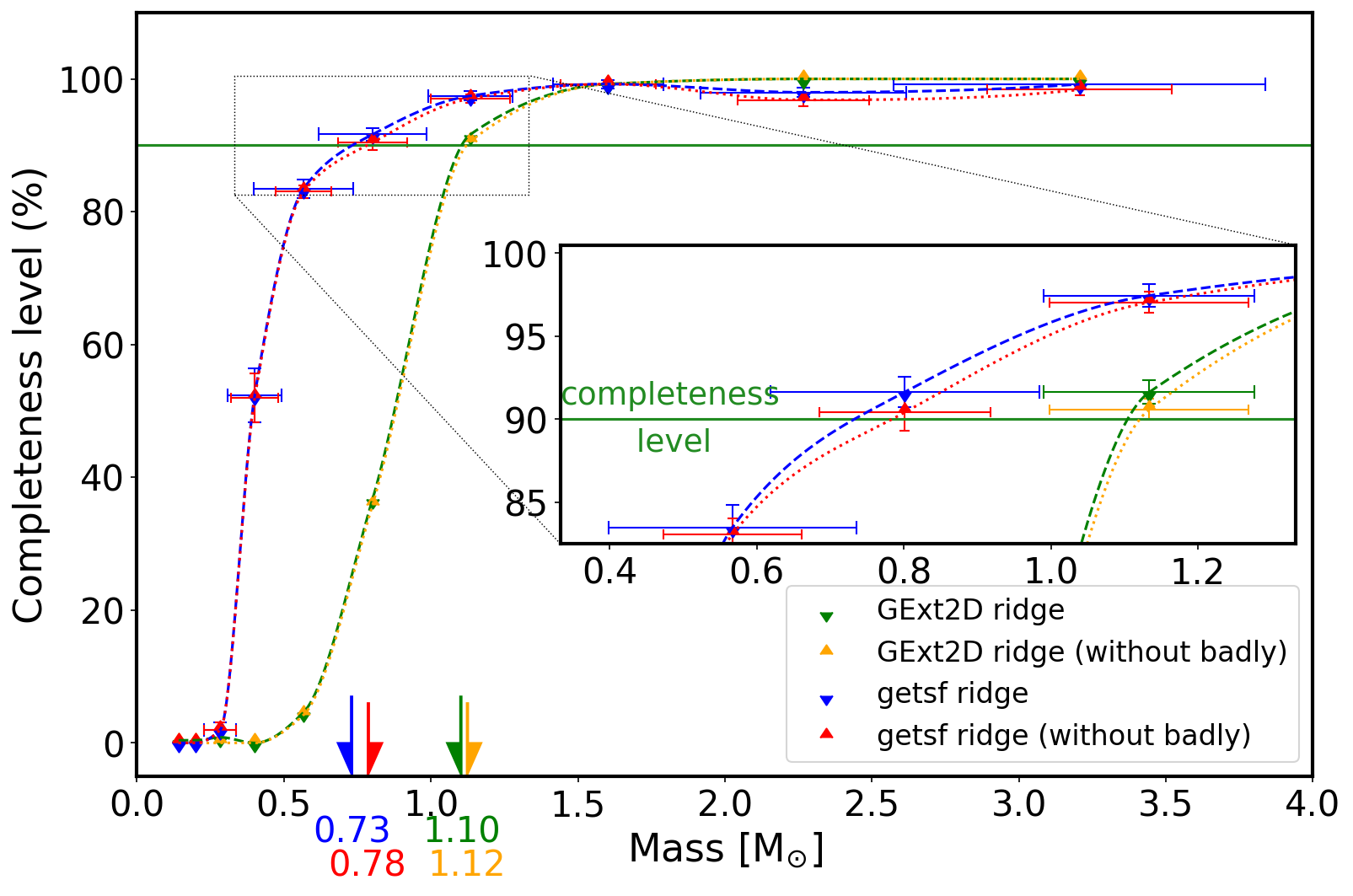
Figure 13: Completeness levels of the $\sim$900 synthetic cores added on the background image of W43-MM2&MM3. The core content is 90% complete down to $0.8\pm 0.2\leavevmode\nobreak\ M_{\odot}$ and $1.1\pm 0.2\leavevmode\nobreak\ M_{\odot}$ for getsf and GExt2D, respectively. The error bars represent the $\pm 1\sigma$ uncertainties for mass estimations across each bin (x-axis) and total of cores retrieved per bin (y-axis). Data points were interpolated using the Piecewise Cubic Hermite Interpolating Polynomial method. Blue and green points represent the full sample of cores detected by getsf and GExt2D, respectively, while red and orange points measure the bin completeness for cores that have mass measurements at worst larger or smaller than a factor of 2 compared to the truth table, thus excluding badly detected sources (see Appendix A and Table 5 for complementary information).

We estimated the completeness level of each of the getsf and Gext2D core catalogs by injecting synthetic populations of $\sim$1900 sources over the background image of W43-MM2&MM3. Background images are produced by getsf during the source extraction process in the denoised & bsens and bsens images at 1.3 mm, respectively (see Sect. 3). Synthetic sources were split into ten bins logarithmically spaced between $0.1\leavevmode\nobreak\ M_{\odot}$ and $3.2\leavevmode\nobreak\ M_{\odot}$, with a constant number of about 190 sources per bin in order to properly sample the bins useful for defining the completeness level. Synthetic sources more massive than $3.2\leavevmode\nobreak\ M_{\odot}$ have a flux contrast to their background that allows their detection in all test cases. The density profile chosen for synthetic cores is Gaussians with FWHM of $0.7\arcsec$ (or 3 400 au at 5.5 kpc), equal to the median size of extracted sources (see Fig. 2), and with an outer diameter of 2.5″. Following Appendix A (see Fig. 10), sources are randomly injected in a regular grid, not allowing cores to overlap. We focus on the $\sim$900 synthetic sources located within the central part of the W43-MM2&MM3 ridge, corresponding to the location of its detected cores (see Fig. 1a). This method allows us to estimate a level of completeness as close as possible to that of our core catalog. With a source grid covering the entire image, the completeness level would be 1.4 times smaller. We performed five series of completeness simulations, varying the location of synthetic sources to mitigate the effects of the chosen grid relative to the background and allow estimation of the error bars of Fig. 13. We ran the extraction algorithms getsf and Gext2D on all these synthetic images with the same parameters as for the observations (see Sect. 3).

Figure 13 shows the detection rates of synthetic sources injected on the W43-MM2&MM3 background image versus the synthetic source mass. We use it to estimate a global 90% completeness level (excluding badly measured sources) of $\sim$0.8$\pm 0.2\leavevmode\nobreak\ M_{\odot}$ for the getsf and $\sim$1.1$\pm 0.2\leavevmode\nobreak\ M_{\odot}$ for the Gext2D catalogs, respectively. Uncertainties are estimated from the error bars shown in Fig. 13 in the mass bins located near the point of intersection with the 90% completeness level. 75% of the sample of Table 7 lie above the getsf completeness level.

Appendix D Complementary figures

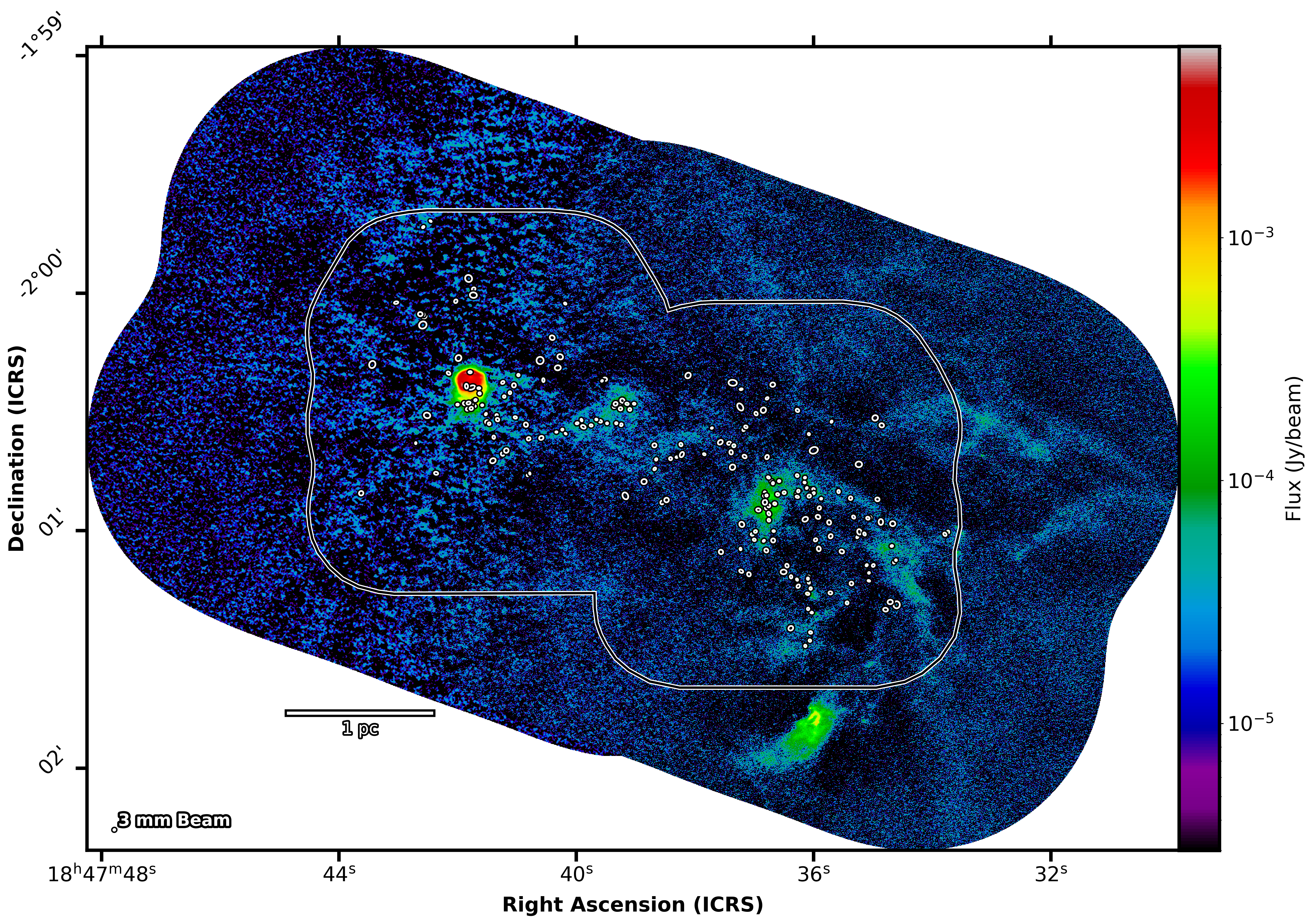
Figure 14: W43-MM2&MM3 protocluster cloud imaged at 3 mm by the ALMA 12 m array (best-sensitivity image prior to primary-beam correction). White ellipses outline the FWHM size of compact cores extracted by getsf at 1.3 mm and whose 3 mm flux is measurable (see Sect. 3). the ellipse in the lower left corner represents the angular resolution of the bsens 3 mm image and the scale bar indicates the size in physical units.

Figure 15: Thermal dust emission cores separated from free-free emission sources, using their 1.3 mm to 3 mm flux ratios without re-scaling, $\gamma_{0}$ (in a), and with a stronger re-scaling suited for the flatter density distribution of starless cores, $\gamma_{2}$ (in b). Plots are shown as a function of the S/N in the 1.3 mm image. The magenta horizontal dashed line represents the theoretical flux ratio of thermal dust emission of 15.4, computed in Eq. 3. The gray segments correspond to the median values of the core flux ratios and the shaded gray area is their $3\,\sigma$ dispersion. Blue points indicate cores with 3 mm thermal dust emission whose flux is re-scaled to the source size measured at 1.3 mm (see Eq. 1), while orange points locate cores undetected at 3 mm, thus taking the ratio between the 1.3 mm peak flux and the $1\,\sigma$ peak error at 3 mm, corresponding to a lower limit. Red symbols are sources located within the H41$\alpha$ recombination line region of Fig. 3a. The gray curve indicates the median value of the core ratios, computed over bins of 20 adjacent cores as ranked by their S/N. The shaded gray area indicates the corresponding $3\,\sigma$ dispersion in flux ratio values. The magenta horizontal dashed line represents the theoretical flux ratio of thermal dust emission of 15.4, computed in Eq. 3. The red hatched area locates the theoretical flux ratios of UCH ii or HCH ii regions, whose free-free emission is either optically thin (lower limit) or partly to totally optically thick (upper limit). The median value of the blue points is $8.4\pm 2.1$ (in a) and $15.3\pm 2.0$ (in b).

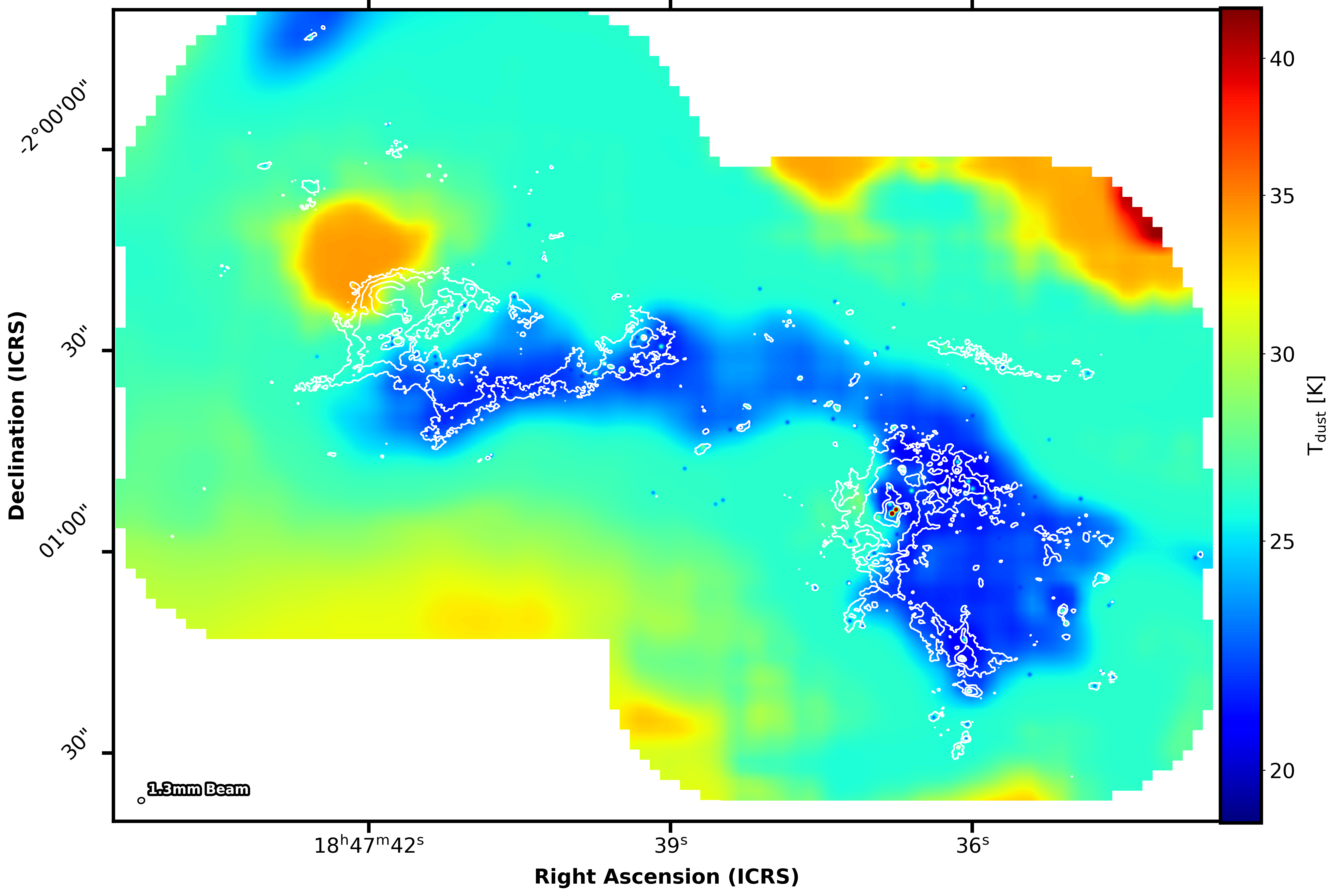
Figure 16: Background dust temperature of the W43-MM2&MM3 protocluster cloud from Motte et al. (in prep.). It combines a $2.5\arcsec$-resolution dust temperature image computed by PPMAP with the central heating and self-shielding of protostellar and pre-stellar cores, respectively, at $0.46\arcsec$ resolution (see Sect. 4.2). White contours correspond to 4, 15, 75, and $150\,\sigma$ of the ALMA 12 m array bsens image, at 1.3 mm.

Appendix D presents the 3 mm continuum image of the W43-MM2&3 ridge (see Fig. 14), complementary figures used to identify sources associated with free-free emission peaks (see Fig. 15), and the dust temperature background image of Motte et al. (in prep.) (see also Sect. 4.2).

Appendix E Online tables

Appendix E presents Tables 6 and 7. The first lists the sources detected by getsf at 1.3 mm and the second gives their physical properties (see Sects. 3 and 4).

[c]

Table 6: Catalog of dense cores identified by getsf (v210403) in the ALMA-IMF images of the W43-MM2&MM3 mini-starburst.

n

Core name

RA

Dec

$a_{\rm 1.3mm}\times b_{\rm 1.3mm}$

PA1.3mm

$S_{\rm 1.3mm}^{\rm peak}$

$S_{\rm 1.3mm}^{\rm int}$

$a_{\rm 3mm}\times b_{\rm 3mm}$

PA3mm

$S_{\rm 3mm}^{\rm peak}$

$S_{\rm 3mm}^{\rm int}$

GExt2D tag

Contamination

W43-MM2&3_ALMAIMF$\ast$

[J2000]

[J2000]

[$\arcsec\times\arcsec$]

[deg]

[mJy beam-1]

[mJy]

[$\arcsec\times\arcsec$]

[deg]

[mJy beam-1]

[mJy]

1

184736.80-20054.27

18:47:36.80

-2:00:54.27

$0.8\times 0.6$

5

$140.00\pm 1.35$

$398.70\pm 3.07$

$0.8\times 0.5$

25

$9.24\pm 0.14$

$23.16\pm 0.20$

$\star\star$

COMs

2

184741.71-20028.60

18:47:41.71

-2:00:28.60

$0.6\times 0.5$

94

$53.73\pm 1.15$

$100.70\pm 1.60$

$0.7\times 0.5$

117

$4.12\pm 0.37$

$7.94\pm 0.66$

$\star\star$

3

184739.26-20028.10

18:47:39.26

-2:00:28.10

$0.7\times 0.6$

23

$17.06\pm 0.35$

$42.18\pm 0.60$

$0.8\times 0.7$

173

$0.86\pm 0.04$

$2.31\pm 0.06$

$\star\star$

COMs

5

184736.10-20115.98

18:47:36.10

-2:01:15.98

$0.9\times 0.6$

75

$15.11\pm 0.40$

$42.42\pm 0.55$

$0.8\times 0.7$

72

$1.25\pm 0.09$

$3.00\pm 0.11$

$\star\star$

6

184736.03-20120.73

18:47:36.03

-2:01:20.73

$0.7\times 0.5$

75

$11.98\pm 0.20$

$20.78\pm 0.21$

$0.6\times 0.5$

57

$1.77\pm 0.09$

$2.43\pm 0.09$

$\star\star$

7

184736.75-20053.75

18:47:36.75

-2:00:53.75

$0.8\times 0.8$

19

$33.85\pm 1.47$

$83.72\pm 1.48$

$0.8\times 0.8$

121

$3.63\pm 0.13$

$9.46\pm 0.13$

COMs

9

184741.73-20027.42

18:47:41.73

-2:00:27.42

$0.6\times 0.5$

108

$26.32\pm 1.02$

$39.18\pm 0.90$

$0.7\times 0.6$

115

$1.75\pm 0.21$

$3.07\pm 0.18$

$\star\star$

10

184736.28-20050.75

18:47:36.28

-2:00:50.75

$0.6\times 0.5$

1

$10.00\pm 0.47$

$15.78\pm 0.45$

$0.6\times 0.5$

5

$1.06\pm 0.06$

$1.74\pm 0.06$

$\star$

COMs

11

184740.97-20020.73

18:47:40.97

-2:00:20.73

$0.6\times 0.6$

34

$6.77\pm 0.25$

$14.63\pm 0.30$

$0.7\times 0.6$

69

$0.51\pm 0.05$

$1.12\pm 0.06$

$\star\star$

12

184736.70-20047.55

18:47:36.70

-2:00:47.55

$0.7\times 0.5$

109

$15.83\pm 0.69$

$26.98\pm 0.82$

$0.6\times 0.6$

102

$1.10\pm 0.08$

$1.70\pm 0.07$

$\star\star$

13

184736.15-20047.87

18:47:36.15

-2:00:47.87

$0.6\times 0.5$

69

$9.53\pm 0.31$

$13.22\pm 0.29$

$0.6\times 0.5$

45

$1.13\pm 0.08$

$1.52\pm 0.07$

$\star\star$

14

184735.10-20108.77

18:47:35.10

-2:01:08.77

$0.6\times 0.5$

134

$5.85\pm 0.19$

$10.60\pm 0.25$

$0.7\times 0.6$

137

$0.82\pm 0.03$

$1.63\pm 0.04$

$\star\star$

15

184736.84-20102.61

18:47:36.84

-2:01:02.61

$0.6\times 0.4$

128

$8.18\pm 0.38$

$11.66\pm 0.39$

$0.9\times 0.6$

156

$0.99\pm 0.06$

$2.61\pm 0.07$

$\star$

16

184735.69-20032.50

18:47:35.69

-2:00:32.50

$0.6\times 0.5$

152

$3.71\pm 0.11$

$6.45\pm 0.15$

$0.6\times 0.5$

104

$0.44\pm 0.03$

$0.87\pm 0.04$

$\star\star$

18

184740.23-20034.51

18:47:40.23

-2:00:34.51

$0.6\times 0.5$

103

$3.83\pm 0.17$

$5.68\pm 0.17$

$0.6\times 0.5$

114

$0.29\pm 0.03$

$0.43\pm 0.03$

$\star\star$

20

184736.06-20127.82

18:47:36.06

-2:01:27.82

$0.7\times 0.6$

56

$4.75\pm 0.21$

$9.56\pm 0.24$

$0.8\times 0.7$

110

$0.57\pm 0.04$

$1.62\pm 0.06$

$\star\star$

21

184741.39-20036.43

18:47:41.39

-2:00:36.43

$0.9\times 0.7$

6

$0.45\pm 0.18$

$1.14\pm 0.18$

–

–

$\leq 0.003$

$\leq 0.003$

$\star$

22

184736.65-20053.23

18:47:36.65

-2:00:53.23

$0.8\times 0.7$

85

$11.67\pm 1.36$

$31.92\pm 1.62$

$0.8\times 0.7$

25

$0.71\pm 0.15$

$1.75\pm 0.18$

$\star$

24

184741.63-20025.37

18:47:41.63

-2:00:25.37

$0.6\times 0.6$

44

$11.09\pm 1.28$

$19.65\pm 1.30$

$0.7\times 0.7$

164

$0.53\pm 0.31$

$1.11\pm 0.31$

$\star\star$

25

184741.83-20029.32

18:47:41.83

-2:00:29.32

$1.0\times 0.8$

117

$9.18\pm 0.96$

$36.75\pm 1.47$

$1.1\times 0.8$

101

$0.42\pm 0.18$

$1.35\pm 0.21$

$\star\star$

27

184741.76-20023.88

18:47:41.76

-2:00:23.88

$1.7\times 1.0$

112

$5.03\pm 1.33$

$33.15\pm 2.30$

$1.6\times 1.1$

116

$6.53\pm 1.46$

$45.93\pm 2.47$

Free-free

28

184736.68-20048.06

18:47:36.68

-2:00:48.06

$0.6\times 0.5$

166

$9.54\pm 0.70$

$15.02\pm 0.61$

$0.6\times 0.5$

167

$0.96\pm 0.08$

$1.41\pm 0.07$

$\star\star$

30

184737.17-20034.45

18:47:37.17

-2:00:34.45

$1.0\times 0.7$

142

$0.43\pm 0.08$

$1.27\pm 0.11$

$1.6\times 1.6$

98

$0.05\pm 0.01$

$0.38\pm 0.02$

32

184738.30-20041.47

18:47:38.30

-2:00:41.47

$0.6\times 0.4$

98

$2.42\pm 0.09$

$3.56\pm 0.10$

$0.6\times 0.5$

81

$0.25\pm 0.02$

$0.36\pm 0.02$

$\star\star$

33

184736.82-20052.88

18:47:36.82

-2:00:52.88

$1.2\times 1.1$

170

$12.63\pm 1.01$

$69.47\pm 1.17$

$1.0\times 0.7$

9

$0.60\pm 0.14$

$2.33\pm 0.13$

34

184736.97-20030.47

18:47:36.97

-2:00:30.47

$1.0\times 0.8$

30

$0.37\pm 0.09$

$1.24\pm 0.10$

–

–

$\leq 0.013$

$\leq 0.020$

35

184733.73-20100.38

18:47:33.73

-2:01:00.38

$0.8\times 0.6$

178

$3.37\pm 0.17$

$7.51\pm 0.20$

$0.9\times 0.6$

98

$0.43\pm 0.05$

$1.25\pm 0.07$

$\star\star$

37

184739.48-20032.93

18:47:39.48

-2:00:32.93

$0.5\times 0.5$

98

$3.75\pm 0.33$

$4.92\pm 0.29$

$0.6\times 0.5$

106

$0.38\pm 0.03$

$0.62\pm 0.03$

$\star\star$

38

184735.05-20056.75

18:47:35.05

-2:00:56.75

$0.8\times 0.8$

13

$0.27\pm 0.10$

$0.79\pm 0.11$

–

–

$\leq 0.016$

$\leq 0.018$

39

184736.14-20046.65

18:47:36.14

-2:00:46.65

$0.6\times 0.4$

104

$3.56\pm 0.26$

$4.22\pm 0.23$

$0.5\times 0.5$

98

$0.55\pm 0.06$

$0.66\pm 0.05$

$\star$

40

184734.99-20108.83

18:47:34.99

-2:01:08.83

$0.8\times 0.7$

136

$0.40\pm 0.11$

$0.91\pm 0.12$

–

–

$\leq 0.019$

$\leq 0.026$

$\star$

41

184736.14-20129.16

18:47:36.14

-2:01:29.16

$0.6\times 0.6$

12

$2.57\pm 0.26$

$5.22\pm 0.30$

$0.7\times 0.6$

106

$0.20\pm 0.05$

$0.43\pm 0.06$

$\star\star$

43

184739.22-20027.20

18:47:39.22

-2:00:27.20

$1.1\times 1.0$

45

$3.43\pm 0.27$

$12.90\pm 0.27$

$0.9\times 0.8$

153

$0.21\pm 0.04$

$0.59\pm 0.04$

$\star\star$

• Notes: RA, right ascension; Dec, declination; $a$ and $b$, major and minor sizes at half maximum; PA, counterclockwise ellipse orientation from north to east; $S^{\rm peak}$ and $S^{\rm int}$, peak and integrated fluxes; $\star$, detected by GExt2D; $\star\star$, detected by GExt2D and with a 1.3 mm integrated flux at worst 30% larger or smaller than getsf fluxes; Contamination, tag to indicate source with partial contamination (COMs, Lines) or almost fully contamined fluxes (free-free). The full table is available in electronic form through CDS.

[c] n Core name FWHM${}^{\rm dec}_{\rm 1.3mm}$ $M_{\rm\tau\gtrsim 1}$ $T_{\rm dust}$ $n_{\rm H_{2}}$ W43-MM2&3_ALMAIMF$\ast$ [AU] [$M_{\odot}$] [K] [$\times 10^{6}$cm^-3] 1 184736.80-20054.27 3070 $69.9\pm 13.7$ $65.0\pm 10.0$ 72.85 2 184741.71-20028.60 1820 $44.6\pm 8.8$ $28.7\pm 4.0$ 223.46 3 184739.26-20028.10 2760 $11.2\pm 2.3$ $40.0\pm 7.0$ 16.25 5 184736.10-20115.98 3330 $17.8\pm 3.3$ $27.5\pm 4.0$ 14.58 6 184736.03-20120.73 1880 $8.5\pm 1.5$ $27.8\pm 4.0$ 38.85 7 184736.75-20053.75 3500 $14.3\pm 1.9$ $60.0\pm 7.0$ 10.05 9 184741.73-20027.42 1780 $16.0\pm 2.9$ $28.7\pm 4.0$ 86.32 10 184736.28-20050.75 1890 $2.6\pm 0.3$ $60.0\pm 7.0$ 11.82 11 184740.97-20020.73 2260 $7.7\pm 1.3$ $22.6\pm 3.0$ 20.19 12 184736.70-20047.55 1840 $11.2\pm 2.1$ $27.8\pm 4.0$ 53.79 13 184736.15-20047.87 1360 $8.2\pm 1.7$ $20.0\pm 3.0$ 98.89 14 184735.10-20108.77 1810 $4.3\pm 0.8$ $27.8\pm 4.0$ 21.79 15 184736.84-20102.61 1530 $4.7\pm 0.9$ $27.8\pm 4.0$ 40.31 16 184735.69-20032.50 1550 $3.4\pm 0.6$ $22.4\pm 3.0$ 27.36 18 184740.23-20034.51 1640 $3.1\pm 0.6$ $21.6\pm 3.0$ 21.29 20 184736.06-20127.82 2560 $4.9\pm 0.8$ $23.0\pm 3.0$ 8.79 21 184741.39-20036.43 3370 $0.6\pm 0.1$ $21.7\pm 3.0$ 0.49 22 184736.65-20053.23 3180 $18.1\pm 3.5$ $21.6\pm 3.0$ 17.02 24 184741.63-20025.37 2230 $7.5\pm 1.3$ $29.4\pm 4.0$ 20.39 25 184741.83-20029.32 4110 $19.6\pm 3.5$ $22.5\pm 3.0$ 8.54 28 184736.68-20048.06 1860 $6.1\pm 1.1$ $27.8\pm 4.0$ 28.83 30 184737.17-20034.45 3850 $0.7\pm 0.1$ $21.9\pm 3.0$ 0.36 32 184738.30-20041.47 1410 $1.9\pm 0.3$ $21.9\pm 3.0$ 20.63 33 184736.82-20052.88 5890 $29.6\pm 5.6$ $26.9\pm 4.0$ 4.39 34 184736.97-20030.47 4080 $0.7\pm 0.1$ $22.1\pm 3.0$ 0.29 35 184733.73-20100.38 2890 $4.0\pm 0.7$ $22.0\pm 3.0$ 5.07 37 184739.48-20032.93 1370 $2.0\pm 0.4$ $27.8\pm 4.0$ 23.13 38 184735.05-20056.75 3580 $0.4\pm 0.1$ $21.8\pm 3.0$ 0.28 39 184736.14-20046.65 1250 $2.4\pm 0.5$ $20.8\pm 3.0$ 38.36 40 184734.99-20108.83 3180 $0.5\pm 0.1$ $21.8\pm 3.0$ 0.46 41 184736.14-20129.16 2250 $1.9\pm 0.3$ $29.9\pm 4.0$ 5.10 43 184739.22-20027.20 5430 $7.0\pm 1.2$ $21.8\pm 3.0$ 1.32

Table 7: Derived properties of cores identified by getsf (v210403) in the ALMA-IMF images of the W43-MM2&MM3 mini-starburst.

• Notes: FWHM^dec, deconvolved physical core size at 1.3 mm; $M_{\rm\tau\gtrsim 1}$, optically thick core dust mass measured from the 1.3 mm integrated flux of Table 6. Uncertainties include 1.3 mm integrated and peak fluxes and uncertainties (see Table 6) and core temperature uncertainty (Col. 5, see Sect. 4.2); $T_{\rm dust}$, dust temperature measured in Fig. 16; $n_{\rm H_{2}}$, volume density of the core (see Eq. 7). The full table is available in electronic form through CDS.