Arbitrarily high-order energy-conserving methods for Hamiltonian problems with quadratic holonomic constraints

P. Amodio Dipartimento di Matematica, Università di Bari, Italy.    L. Brugnano Dipartimento di Matematica e Informatica “U. Dini”, Università di Firenze, Italy.    G. Frasca-Caccia Dipartimento di Matematica, Università di Salerno, Italy.    F. Iavernaro 11footnotemark: 1
Abstract

In this paper, we define arbitrarily high-order energy-conserving methods for Hamiltonian systems with quadratic holonomic constraints. The derivation of the methods is made within the so-called line integral framework. Numerical tests to illustrate the theoretical findings are presented.

Keywords: constrained Hamiltonian systems; quadratic holonomic constraints; energy-conserving methods; line integral methods; Hamiltonian Boundary Value Methods; HBVMs.

MSC: 65P10, 65L80, 65L06.

1 Introduction

In recent years, much interest has been given to the modeling and/or simulation of tethered systems, where the dynamics of interconnected bodies is studied (see, e.g. [26, 41, 24, 25, 43, 44, 40, 42, 2, 32, 33]). It turns out that the underlying dynamics is often described by a Hamiltonian system, for which the total energy is conserved.

Motivated by this fact, we here investigate the numerical approximation of a constrained Hamiltonian dynamics, described by the separable Hamiltonian

H(q,p)=12pM1pU(q),q,pm,formulae-sequence𝐻𝑞𝑝12superscript𝑝topsuperscript𝑀1𝑝𝑈𝑞𝑞𝑝superscript𝑚H(q,p)=\frac{1}{2}p^{\top}M^{-1}p-U(q),\qquad q,p\in\mathbb{R}^{m}, (1)

where M𝑀M is a symmetric and positive-definite (spd) matrix, subject to ν𝜈\nu quadratic holonomic constraints,

g(q)=0ν,νm,formulae-sequence𝑔𝑞0superscript𝜈𝜈𝑚g(q)=0\in\mathbb{R}^{\nu},\qquad\nu\leq m, (2)

i.e., the entries of g𝑔g are quadratic polynomials. Hereafter, we shall assume all points be regular for the constraints, i.e., g(q)m×ν𝑔𝑞superscript𝑚𝜈\nabla g(q)\in\mathbb{R}^{m\times\nu} has full column rank or, equivalently,

g(q)M1g(q)ν×νis spd.𝑔superscript𝑞topsuperscript𝑀1𝑔𝑞superscript𝜈𝜈is spd\nabla g(q)^{\top}M^{-1}\nabla g(q)\in\mathbb{R}^{\nu\times\nu}\qquad\mbox{is~{}spd}. (3)

Moreover, we shall assume that its smallest eigenvalue is bounded away from 0, in the domain of interest. Also, for sake of simplicity, in the same domain the potential U𝑈U will be assumed to be analytic.

It is well-known that the problem defined by (1)–(2) can be cast in Hamiltonian form by defining the augmented Hamiltonian

H^(q,p,λ)=H(q,p)+λg(q),^𝐻𝑞𝑝𝜆𝐻𝑞𝑝superscript𝜆top𝑔𝑞\hat{H}(q,p,\lambda)=H(q,p)+\lambda^{\top}g(q), (4)

where λ𝜆\lambda is the vector of the Lagrange multipliers. The resulting constrained Hamiltonian system reads:

q˙=M1p,p˙=U(q)g(q)λ,g(q)=0,t[0,T],formulae-sequence˙𝑞superscript𝑀1𝑝formulae-sequence˙𝑝𝑈𝑞𝑔𝑞𝜆formulae-sequence𝑔𝑞0𝑡0𝑇\dot{q}=M^{-1}p,\qquad\dot{p}=\nabla U(q)-\nabla g(q)\lambda,\qquad g(q)=0,\qquad t\in[0,T], (5)

and is subject to consistent initial conditions,

q(0)=q0,p(0)=p0,formulae-sequence𝑞0subscript𝑞0𝑝0subscript𝑝0q(0)=q_{0},\qquad p(0)=p_{0}, (6)

such that

g(q0)=0,g(q0)M1p0=0.formulae-sequence𝑔subscript𝑞00𝑔superscriptsubscript𝑞0topsuperscript𝑀1subscript𝑝00g(q_{0})=0,\qquad\nabla g(q_{0})^{\top}M^{-1}p_{0}=0. (7)

Clearly, H(q,p)H^(q,p,λ)𝐻𝑞𝑝^𝐻𝑞𝑝𝜆H(q,p)\equiv\hat{H}(q,p,\lambda), provided that the constraints (2) are satisfied, and a straightforward calculation proves that both are conserved along the solution trajectory.

We notice that the condition g(q0)=0𝑔subscript𝑞00g(q_{0})=0 ensures that q0subscript𝑞0q_{0} belongs to the manifold

={qm:g(q)=0},conditional-set𝑞superscript𝑚𝑔𝑞0{\cal M}=\left\{q\in\mathbb{R}^{m}:g(q)=0\right\}, (8)

as required by the constraints, whereas the condition g(q0)M1p0𝑔superscriptsubscript𝑞0topsuperscript𝑀1subscript𝑝0\nabla g(q_{0})^{\top}M^{-1}p_{0} means that the motion initially stays on the tangent space to {\cal M} at q0subscript𝑞0q_{0}. This condition is satisfied by all points on the solution trajectory, since, in order for the constraints to be conserved, the following condition needs to be satisfied as well:

g˙(q)=g(q)q˙=g(q)M1p=0ν.˙𝑔𝑞𝑔superscript𝑞top˙𝑞𝑔superscript𝑞topsuperscript𝑀1𝑝0superscript𝜈\dot{g}(q)=\nabla g(q)^{\top}\dot{q}=\nabla g(q)^{\top}M^{-1}p=0\in\mathbb{R}^{\nu}. (9)

These latter constraints are usually referred to as hidden constraints, and allow the derivation of the vector of the Lagrange multiplier λ𝜆\lambda. In fact, from (9) and (5)-(6), one obtains

00\displaystyle 0 =\displaystyle= g(q(t))M1p(t)𝑔superscript𝑞𝑡topsuperscript𝑀1𝑝𝑡\displaystyle\nabla g(q(t))^{\top}M^{-1}p(t) (10)
=\displaystyle= g(q(t))M1[p0+0tU(q(ζ))dζ0tg(q(ζ))λ(ζ)dζ],𝑔superscript𝑞𝑡topsuperscript𝑀1delimited-[]subscript𝑝0superscriptsubscript0𝑡𝑈𝑞𝜁differential-d𝜁superscriptsubscript0𝑡𝑔𝑞𝜁𝜆𝜁differential-d𝜁\displaystyle\nabla g(q(t))^{\top}M^{-1}\left[p_{0}+\int_{0}^{t}\nabla U(q(\zeta))\mathrm{d}\zeta-\int_{0}^{t}\nabla g(q(\zeta))\lambda(\zeta)\mathrm{d}\zeta\right],

from which one derives the integral equation:

g(q(t))M10tg(q(ζ))λ(ζ)dζ𝑔superscript𝑞𝑡topsuperscript𝑀1superscriptsubscript0𝑡𝑔𝑞𝜁𝜆𝜁differential-d𝜁\displaystyle\nabla g(q(t))^{\top}M^{-1}\int_{0}^{t}\nabla g(q(\zeta))\lambda(\zeta)\mathrm{d}\zeta (11)
=\displaystyle= g(q(t))M1[p0+0tU(q(ζ))dζ].𝑔superscript𝑞𝑡topsuperscript𝑀1delimited-[]subscript𝑝0superscriptsubscript0𝑡𝑈𝑞𝜁differential-d𝜁\displaystyle\nabla g(q(t))^{\top}M^{-1}\left[p_{0}+\int_{0}^{t}\nabla U(q(\zeta))\mathrm{d}\zeta\right].
Remark 1

From (10)-(11), one deduces that the vector of the Lagrange multipliers depends on the functions q𝑞q and p𝑝p. We shall denote this by using the notation:

λ(t):=λ(q(t),p(t)).assign𝜆𝑡𝜆𝑞𝑡𝑝𝑡\lambda(t):=\lambda(q(t),p(t)). (12)

We stress that the condition (9) can be conveniently relaxed for a numerical approximation: in fact, we only ask for g(q)M1p𝑔superscript𝑞topsuperscript𝑀1𝑝\nabla g(q)^{\top}M^{-1}p to be suitably small along the numerical solution. Consequently, when solving the problem on the interval [0,h]0[0,h], we require that the approximations,

q1q(h),p1p(h),formulae-sequencesubscript𝑞1𝑞subscript𝑝1𝑝q_{1}\approx q(h),\qquad p_{1}\approx p(h), (13)

satisfy the conservation of both the Hamiltonian and the constraints,

H(q1,p1)=H(q0,p0),g(q1)=0,formulae-sequence𝐻subscript𝑞1subscript𝑝1𝐻subscript𝑞0subscript𝑝0𝑔subscript𝑞10H(q_{1},p_{1})=H(q_{0},p_{0}),\qquad g(q_{1})=0, (14)

whereas the hidden constraints, see (9), become:

g(q(h))M1p(h)=O(hr¯),𝑔superscript𝑞topsuperscript𝑀1𝑝𝑂superscript¯𝑟\nabla g(q(h))^{\top}M^{-1}p(h)=O(h^{\bar{r}}), (15)

for a convenient r¯1¯𝑟1\bar{r}\geq 1.

For sake of completeness, we recall that a formal expression for the vector λ𝜆\lambda is obtained by further differentiating (9):

g¨(q)=2g(q)(M1p,M1p)+g(q)M1[U(q)g(q)λ].¨𝑔𝑞superscript2𝑔𝑞superscript𝑀1𝑝superscript𝑀1𝑝𝑔superscript𝑞topsuperscript𝑀1delimited-[]𝑈𝑞𝑔𝑞𝜆\ddot{g}(q)=\nabla^{2}g(q)(M^{-1}p,M^{-1}p)+\nabla g(q)^{\top}M^{-1}\left[\nabla U(q)-\nabla g(q)\lambda\right]. (16)

In fact, by imposing the vanishing of this derivative yields

[g(q)M1g(q)]λ=2g(q)(M1p,M1p)+g(q)M1U(q).delimited-[]𝑔superscript𝑞topsuperscript𝑀1𝑔𝑞𝜆superscript2𝑔𝑞superscript𝑀1𝑝superscript𝑀1𝑝𝑔superscript𝑞topsuperscript𝑀1𝑈𝑞\left[\nabla g(q)^{\top}M^{-1}\nabla g(q)\right]\lambda~{}=~{}\nabla^{2}g(q)(M^{-1}p,M^{-1}p)+\nabla g(q)^{\top}M^{-1}\nabla U(q). (17)

Consequently, the following result follows.

Theorem 1

The vector λ𝜆\lambda exists and is uniquely determined, provided that (3) holds true. In fact, in such a case, from (17), we obtain

λ=[g(q)M1g(q)]1[2g(q)(M1p,M1p)+g(q)M1U(q)].𝜆superscriptdelimited-[]𝑔superscript𝑞topsuperscript𝑀1𝑔𝑞1delimited-[]superscript2𝑔𝑞superscript𝑀1𝑝superscript𝑀1𝑝𝑔superscript𝑞topsuperscript𝑀1𝑈𝑞\lambda=\left[\nabla g(q)^{\top}M^{-1}\nabla g(q)\right]^{-1}\left[\nabla^{2}g(q)(M^{-1}p,M^{-1}p)+\nabla g(q)^{\top}M^{-1}\nabla U(q)\right].

The numerical solution of Hamiltonian problems with holonomic constraints has been the subject of several investigations across the years. Among the proposed approaches, we mention: the popular Shake-Rattle method [38, 1], later proved to be symplectic [29]; higher order methods obtained via symplectic PRK methods [23]; composition methods [34, 35]; symmetric LMFs [17]; methods based on discrete derivatives [18]; local parametrizations of the manifold containing the solution [3]; projection techniques [36, 39]. As additional references, we refer to [27, 37, 19, 30, 31] and to the monographs [4, 28, 20, 21], and references therein.

In this paper we pursue a different approach, utilizing the so-called line integral framework, which has already been used for deriving the energy-conserving Runge-Kutta methods, for unconstrained Hamiltonian systems, named Hamiltonian Boundary Value Methods (HBVMs) [9, 10, 11, 12, 13], see also the monograph [7] and the review paper [8]. This approach has been already used in [6] for deriving energy-conserving methods for constrained Hamiltonian problems which, however, are in general only second-order accurate. In this paper we propose a class of arbitrarily high-order energy conserving methods for constrained Hamiltonian dynamics, in the relevant case where the constraints are quadratic. As matter of fact, the proposed methods provide approximations (13) satisfying (14) and(15) with r¯¯𝑟\bar{r} arbitrarily large.

With this premise, the structure of the paper is as follows: in Section 2 we define the polynomial approximation defining the basic step of application of the method also studying its conservation properties; in Section 3 we study the order of convergence of the method; in Section 4 we discuss its fully discrete implementation; numerical examples are reported in Section 5; at last, some concluding remarks are given in Section 6.

2 Polynomial approximation

Let us consider the following orthonormal polynomial basis,111As is usual, ΠjsubscriptΠ𝑗\Pi_{j} is the vector space of polynomials of degree j𝑗j, and δijsubscript𝛿𝑖𝑗\delta_{ij} is the Kronecker symbol.

PjΠj,01Pi(x)Pj(x)dx=δij,i,j=0,1,,formulae-sequencesubscript𝑃𝑗subscriptΠ𝑗formulae-sequencesuperscriptsubscript01subscript𝑃𝑖𝑥subscript𝑃𝑗𝑥differential-d𝑥subscript𝛿𝑖𝑗for-all𝑖𝑗01P_{j}\in\Pi_{j},\qquad\int_{0}^{1}P_{i}(x)P_{j}(x)\mathrm{d}x=\delta_{ij},\qquad\forall i,j=0,1,\dots, (18)

given by the shifted and scaled Legendre polynomials, and the infinite expansions on the interval [0,h]0[0,h] (see (5)):

p(ch)=j0Pj(c)γj(p),U(q(ch))=j0Pj(c)ψj(q),c[0,1],formulae-sequence𝑝𝑐subscript𝑗0subscript𝑃𝑗𝑐subscript𝛾𝑗𝑝formulae-sequence𝑈𝑞𝑐subscript𝑗0subscript𝑃𝑗𝑐subscript𝜓𝑗𝑞𝑐01p(ch)=\sum_{j\geq 0}P_{j}(c)\gamma_{j}(p),\quad\nabla U(q(ch))=\sum_{j\geq 0}P_{j}(c)\psi_{j}(q),\quad c\in[0,1], (19)

where, for all j=0,1,𝑗01j=0,1,\dots,

γj(p)=01Pj(ζ)p(ζh)dζ,ψj(q)=01Pj(ζ)U(q(ζh))dζ.formulae-sequencesubscript𝛾𝑗𝑝superscriptsubscript01subscript𝑃𝑗𝜁𝑝𝜁differential-d𝜁subscript𝜓𝑗𝑞superscriptsubscript01subscript𝑃𝑗𝜁𝑈𝑞𝜁differential-d𝜁\gamma_{j}(p)=\int_{0}^{1}P_{j}(\zeta)p(\zeta h)\mathrm{d}\zeta,\qquad\psi_{j}(q)=\int_{0}^{1}P_{j}(\zeta)\nabla U(q(\zeta h))\mathrm{d}\zeta. (20)

In order to derive polynomial approximations u𝑢u and v𝑣v of degree s𝑠s,

u(ch)q(ch),v(ch)p(ch),c[0,1],formulae-sequence𝑢𝑐𝑞𝑐formulae-sequence𝑣𝑐𝑝𝑐𝑐01u(ch)\approx q(ch),\qquad v(ch)\approx p(ch),\qquad c\in[0,1],

we shall consider the following approximation to (5) on the interval [0,h]0[0,h],

u˙(ch)˙𝑢𝑐\displaystyle\dot{u}(ch) =\displaystyle= M1j=0s1Pj(c)γj(v),u(0)=q0,c[0,1],formulae-sequencesuperscript𝑀1superscriptsubscript𝑗0𝑠1subscript𝑃𝑗𝑐subscript𝛾𝑗𝑣𝑢0subscript𝑞0𝑐01\displaystyle M^{-1}\sum_{j=0}^{s-1}P_{j}(c)\gamma_{j}(v),\qquad u(0)=q_{0},\qquad c\in[0,1],
v˙(ch)˙𝑣𝑐\displaystyle\dot{v}(ch) =\displaystyle= j=0s1Pj(c)ψj(u)j=1sj(c)ρj,v(0)=p0,superscriptsubscript𝑗0𝑠1subscript𝑃𝑗𝑐subscript𝜓𝑗𝑢superscriptsubscript𝑗1𝑠subscript𝑗𝑐subscript𝜌𝑗𝑣0subscript𝑝0\displaystyle\sum_{j=0}^{s-1}P_{j}(c)\psi_{j}(u)-\sum_{j=1}^{s}\ell_{j}(c)\rho_{j},\qquad v(0)=p_{0}, (21)
ρjsubscript𝜌𝑗\displaystyle\rho_{j} :=assign\displaystyle:= g(u(cjh))λj,j=1,,s,formulae-sequence𝑔𝑢subscript𝑐𝑗subscript𝜆𝑗𝑗1𝑠\displaystyle\nabla g(u(c_{j}h))\lambda_{j},\qquad j=1,\dots,s,

where:

  • γj(v)subscript𝛾𝑗𝑣\gamma_{j}(v) and ψj(u)subscript𝜓𝑗𝑢\psi_{j}(u) are defined according to (20), by formally replacing q𝑞q and p𝑝p with u𝑢u and v𝑣v, respectively;

  • 0<c1<<cs<10subscript𝑐1subscript𝑐𝑠10<c_{1}<\dots<c_{s}<1  are the zeros of  Ps(c)subscript𝑃𝑠𝑐P_{s}(c),  Ps(cj)=0subscript𝑃𝑠subscript𝑐𝑗0P_{s}(c_{j})=0,  j=1,,s𝑗1𝑠j=1,\dots,s;

  • j(c)subscript𝑗𝑐\ell_{j}(c) are the Lagrange polynomials defined over the previous abscissae;

  • finally, by using the notation (12),

    λjλ¯(cjh):=λ(u(cjh),v(cjh))subscript𝜆𝑗¯𝜆subscript𝑐𝑗assign𝜆𝑢subscript𝑐𝑗𝑣subscript𝑐𝑗\lambda_{j}\approx\bar{\lambda}(c_{j}h):=\lambda(u(c_{j}h),v(c_{j}h)) (22)

    are approximation to the Lagrange multipliers, which will be defined in the sequel.

Moreover, let us denote by

bj=01j(c)dc,j=1,,s,formulae-sequencesubscript𝑏𝑗superscriptsubscript01subscript𝑗𝑐differential-d𝑐𝑗1𝑠b_{j}=\int_{0}^{1}\ell_{j}(c)\mathrm{d}c,\qquad j=1,\dots,s,

the weights of the Gauss-Legendre quadrature of order 2s2𝑠2s. The new approximations,

q1:=u(h),p1:=v(h),formulae-sequenceassignsubscript𝑞1𝑢assignsubscript𝑝1𝑣q_{1}:=u(h),\qquad p_{1}:=v(h), (23)

will be then defined such that (14) and (15) are satisfied, for a convenient r¯¯𝑟\bar{r} depending on s𝑠s.

For later use, we observe that, at the Gauss-Legendre abscissae {ci}subscript𝑐𝑖\{c_{i}\}, (21) reads:

u˙(cih)˙𝑢subscript𝑐𝑖\displaystyle\dot{u}(c_{i}h) =\displaystyle= M1v(cih),superscript𝑀1𝑣subscript𝑐𝑖\displaystyle M^{-1}v(c_{i}h), (24)
v˙(cih)˙𝑣subscript𝑐𝑖\displaystyle\dot{v}(c_{i}h) =\displaystyle= j=0s1Pj(ci)ψj(u)g(u(cih))λi,i=1,,s.formulae-sequencesuperscriptsubscript𝑗0𝑠1subscript𝑃𝑗subscript𝑐𝑖subscript𝜓𝑗𝑢𝑔𝑢subscript𝑐𝑖subscript𝜆𝑖𝑖1𝑠\displaystyle\sum_{j=0}^{s-1}P_{j}(c_{i})\psi_{j}(u)-\nabla g(u(c_{i}h))\lambda_{i},\qquad i=1,\dots,s.

In fact, since v(ch)Πs𝑣𝑐subscriptΠ𝑠v(ch)\in\Pi_{s}, then (see (20))

v(ch)=j=0sPj(c)γj(v),c[0,1],formulae-sequence𝑣𝑐superscriptsubscript𝑗0𝑠subscript𝑃𝑗𝑐subscript𝛾𝑗𝑣𝑐01v(ch)=\sum_{j=0}^{s}P_{j}(c)\gamma_{j}(v),\qquad c\in[0,1],

however, at the zeros of Pssubscript𝑃𝑠P_{s}, one obviously has:

v(cih)=j=0s1Pj(ci)γj(v),i=1,,s.formulae-sequence𝑣subscript𝑐𝑖superscriptsubscript𝑗0𝑠1subscript𝑃𝑗subscript𝑐𝑖subscript𝛾𝑗𝑣𝑖1𝑠v(c_{i}h)=\sum_{j=0}^{s-1}P_{j}(c_{i})\gamma_{j}(v),\qquad i=1,\dots,s. (25)

2.1 Constraints conservation

Let us now study the conservation of the holonomic constraints in (14), i.e. under which conditions g(q1)=0𝑔subscript𝑞10g(q_{1})=0. One has, by virtue of (24):

g(q1)𝑔subscript𝑞1\displaystyle g(q_{1}) \displaystyle\equiv g(u(h))=h01g(u(ch))u˙(ch)dc𝑔𝑢superscriptsubscript01𝑔superscript𝑢𝑐top˙𝑢𝑐differential-d𝑐\displaystyle g(u(h))~{}=~{}h\int_{0}^{1}\nabla g(u(ch))^{\top}\dot{u}(ch)\mathrm{d}c
=\displaystyle= hi=1sbig(u(cih))u˙(cih)=hi=1sbig(u(cih))M1v(cih),superscriptsubscript𝑖1𝑠subscript𝑏𝑖𝑔superscript𝑢subscript𝑐𝑖top˙𝑢subscript𝑐𝑖superscriptsubscript𝑖1𝑠subscript𝑏𝑖𝑔superscript𝑢subscript𝑐𝑖topsuperscript𝑀1𝑣subscript𝑐𝑖\displaystyle h\sum_{i=1}^{s}b_{i}\nabla g(u(c_{i}h))^{\top}\dot{u}(c_{i}h)~{}=~{}h\sum_{i=1}^{s}b_{i}\nabla g(u(c_{i}h))^{\top}M^{-1}v(c_{i}h),\qquad\quad

where the third equality follows from the fact that the integrand has degree 2s12𝑠12s-1, and the last equality follows from (24). Consequently, the following result is proved.

Theorem 2

g(q1)=0𝑔subscript𝑞10g(q_{1})=0, provided that:

g(u(cih))M1v(cih)=0ν,i=1,,s.formulae-sequence𝑔superscript𝑢subscript𝑐𝑖topsuperscript𝑀1𝑣subscript𝑐𝑖0superscript𝜈𝑖1𝑠\nabla g(u(c_{i}h))^{\top}M^{-1}v(c_{i}h)=0\in\mathbb{R}^{\nu},\qquad i=1,\dots,s. (26)

2.2 Energy conservation

Let us now study the conservation of the Hamiltonian function (1). By using the usual line integral argument, from (21) one has:

H(q1,p1)H(q0,p0)H(u(h),v(h))H(u(0),v(0))𝐻subscript𝑞1subscript𝑝1𝐻subscript𝑞0subscript𝑝0𝐻𝑢𝑣𝐻𝑢0𝑣0\displaystyle H(q_{1},p_{1})-H(q_{0},p_{0})~{}\equiv~{}H(u(h),v(h))-H(u(0),v(0))
=\displaystyle= 0hddtH(u(t),v(t))dtsuperscriptsubscript0dd𝑡𝐻𝑢𝑡𝑣𝑡differential-d𝑡\displaystyle\int_{0}^{h}\frac{\mathrm{d}}{\mathrm{d}t}H(u(t),v(t))\mathrm{d}t
=\displaystyle= h01[Hq(u(ch),v(ch))u˙(ch)+Hp(u(ch),v(ch))v˙(ch)]dcsuperscriptsubscript01delimited-[]subscript𝐻𝑞superscript𝑢𝑐𝑣𝑐top˙𝑢𝑐subscript𝐻𝑝superscript𝑢𝑐𝑣𝑐top˙𝑣𝑐differential-d𝑐\displaystyle h\int_{0}^{1}\left[H_{q}(u(ch),v(ch))^{\top}\dot{u}(ch)+H_{p}(u(ch),v(ch))^{\top}\dot{v}(ch)\right]\mathrm{d}c
=\displaystyle= h01[U(u(ch))M1j=0s1Pj(c)γj(v)+v(ch)M1j=0s1Pj(c)ψj(u)\displaystyle h\int_{0}^{1}\left[-\nabla U(u(ch))^{\top}M^{-1}\sum_{j=0}^{s-1}P_{j}(c)\gamma_{j}(v)+v(ch)^{\top}M^{-1}\sum_{j=0}^{s-1}P_{j}(c)\psi_{j}(u)\right.
v(ch)M1j=1sj(c)ρj]dc\displaystyle\left.\qquad~{}~{}-~{}v(ch)^{\top}M^{-1}\sum_{j=1}^{s}\ell_{j}(c)\rho_{j}\right]\mathrm{d}c
=\displaystyle= hj=0s1[01Pj(c)U(u(ch))dc]=ψj(u)M1γj(v)superscriptsubscript𝑗0𝑠1superscriptsuperscriptdelimited-[]superscriptsubscript01subscript𝑃𝑗𝑐𝑈𝑢𝑐differential-d𝑐topabsentsubscript𝜓𝑗superscript𝑢topsuperscript𝑀1subscript𝛾𝑗𝑣\displaystyle-~{}h\sum_{j=0}^{s-1}\overbrace{\left[\int_{0}^{1}P_{j}(c)\nabla U(u(ch))\mathrm{d}c\right]^{\top}}^{=\psi_{j}(u)^{\top}}M^{-1}\gamma_{j}(v)
+hj=0s1[01Pj(c)v(ch)dc]=γj(v)M1ψj(u)h01j=1sv(ch)M1j(c)ρjdcsuperscriptsubscript𝑗0𝑠1superscriptsuperscriptdelimited-[]superscriptsubscript01subscript𝑃𝑗𝑐𝑣𝑐differential-d𝑐topabsentsubscript𝛾𝑗superscript𝑣topsuperscript𝑀1subscript𝜓𝑗𝑢superscriptsubscript01superscriptsubscript𝑗1𝑠𝑣superscript𝑐topsuperscript𝑀1subscript𝑗𝑐subscript𝜌𝑗d𝑐\displaystyle+~{}h\sum_{j=0}^{s-1}\overbrace{\left[\int_{0}^{1}P_{j}(c)v(ch)\mathrm{d}c\right]^{\top}}^{=\gamma_{j}(v)^{\top}}M^{-1}\psi_{j}(u)-h\int_{0}^{1}\sum_{j=1}^{s}v(ch)^{\top}M^{-1}\ell_{j}(c)\rho_{j}\mathrm{d}c
=\displaystyle= hj=0s1ψj(u)M1γj(v)+hj=0s1γj(v)M1ψj(u)hi=1sbiv(cih)M1ρisuperscriptsubscript𝑗0𝑠1subscript𝜓𝑗superscript𝑢topsuperscript𝑀1subscript𝛾𝑗𝑣superscriptsubscript𝑗0𝑠1subscript𝛾𝑗superscript𝑣topsuperscript𝑀1subscript𝜓𝑗𝑢superscriptsubscript𝑖1𝑠subscript𝑏𝑖𝑣superscriptsubscript𝑐𝑖topsuperscript𝑀1subscript𝜌𝑖\displaystyle-h\sum_{j=0}^{s-1}\psi_{j}(u)^{\top}M^{-1}\gamma_{j}(v)+h\sum_{j=0}^{s-1}\gamma_{j}(v)^{\top}M^{-1}\psi_{j}(u)-h\sum_{i=1}^{s}b_{i}v(c_{i}h)^{\top}M^{-1}\rho_{i}
=\displaystyle= hi=1sbiv(cih)M1g(u(cih))λi.superscriptsubscript𝑖1𝑠subscript𝑏𝑖𝑣superscriptsubscript𝑐𝑖topsuperscript𝑀1𝑔𝑢subscript𝑐𝑖subscript𝜆𝑖\displaystyle-h\sum_{i=1}^{s}b_{i}v(c_{i}h)^{\top}M^{-1}\nabla g(u(c_{i}h))\lambda_{i}.

In fact, considering that the Gauss-Legendre formula has order 2s2𝑠2s,

01j=1sv(ch)M1j(c)ρjdc=i,j=1sbiv(cih)M1j(ci)ρjsuperscriptsubscript01superscriptsubscript𝑗1𝑠𝑣superscript𝑐topsuperscript𝑀1subscript𝑗𝑐subscript𝜌𝑗d𝑐superscriptsubscript𝑖𝑗1𝑠subscript𝑏𝑖𝑣superscriptsubscript𝑐𝑖topsuperscript𝑀1subscript𝑗subscript𝑐𝑖subscript𝜌𝑗\displaystyle\int_{0}^{1}\sum_{j=1}^{s}v(ch)^{\top}M^{-1}\ell_{j}(c)\rho_{j}\mathrm{d}c~{}=~{}\sum_{i,j=1}^{s}b_{i}v(c_{i}h)^{\top}M^{-1}\ell_{j}(c_{i})\rho_{j}
=\displaystyle= i=1sbiv(cih)M1ρi=i=1sbiv(cih)M1g(u(cih))λi.superscriptsubscript𝑖1𝑠subscript𝑏𝑖𝑣superscriptsubscript𝑐𝑖topsuperscript𝑀1subscript𝜌𝑖superscriptsubscript𝑖1𝑠subscript𝑏𝑖𝑣superscriptsubscript𝑐𝑖topsuperscript𝑀1𝑔𝑢subscript𝑐𝑖subscript𝜆𝑖\displaystyle\sum_{i=1}^{s}b_{i}v(c_{i}h)^{\top}M^{-1}\rho_{i}~{}=~{}\sum_{i=1}^{s}b_{i}v(c_{i}h)^{\top}M^{-1}\nabla g(u(c_{i}h))\lambda_{i}.

Consequently, the following result is proved.

Theorem 3

Assume that the conditions (26) hold true. Then, H(q1,p1)=H(q0,p0)𝐻subscript𝑞1subscript𝑝1𝐻subscript𝑞0subscript𝑝0H(q_{1},p_{1})=H(q_{0},p_{0}), i.e., the energy is conserved.

2.3 Computing the approximate Lagrange multipliers

Before studying the accuracy of the approximations (13) and (23), let us derive the algebraic formulation of the conditions (26), i.e., the discrete analog of (10) at t=cih𝑡subscript𝑐𝑖t=c_{i}h, i=1,,s𝑖1𝑠i=1,\dots,s. For this purpose, let us define the following matrices,

𝒈𝒈\displaystyle\nabla\bm{g} =\displaystyle= (g(u(c1h))g(u(csh)))sm×sν𝑔𝑢subscript𝑐1missing-subexpressionmissing-subexpressionmissing-subexpressionmissing-subexpressionmissing-subexpressionmissing-subexpression𝑔𝑢subscript𝑐𝑠superscript𝑠𝑚𝑠𝜈\displaystyle\left(\begin{array}[]{ccc}\nabla g(u(c_{1}h))&&\\ &\ddots\\ &&\nabla g(u(c_{s}h))\end{array}\right)\in\mathbb{R}^{sm\times s\nu} (30)
𝒫ssubscript𝒫𝑠\displaystyle{\cal P}_{s} =\displaystyle= (P0(c1)Ps1(c1)P0(cs)Ps1(cs))s×s,subscript𝑃0subscript𝑐1subscript𝑃𝑠1subscript𝑐1missing-subexpressionsubscript𝑃0subscript𝑐𝑠subscript𝑃𝑠1subscript𝑐𝑠superscript𝑠𝑠\displaystyle\left(\begin{array}[]{ccc}P_{0}(c_{1})&\dots&P_{s-1}(c_{1})\\ \vdots&&\vdots\\ P_{0}(c_{s})&\dots&P_{s-1}(c_{s})\end{array}\right)\in\mathbb{R}^{s\times s}, (34)
ssubscript𝑠\displaystyle{\cal I}_{s} =\displaystyle= (0c1P0(x)dx0c1Ps1(x)dx0csP0(x)dx0csPs1(x)dx)s×s,superscriptsubscript0subscript𝑐1subscript𝑃0𝑥differential-d𝑥superscriptsubscript0subscript𝑐1subscript𝑃𝑠1𝑥differential-d𝑥missing-subexpressionsuperscriptsubscript0subscript𝑐𝑠subscript𝑃0𝑥differential-d𝑥superscriptsubscript0subscript𝑐𝑠subscript𝑃𝑠1𝑥differential-d𝑥superscript𝑠𝑠\displaystyle\left(\begin{array}[]{ccc}\int_{0}^{c_{1}}P_{0}(x)\mathrm{d}x&\dots&\int_{0}^{c_{1}}P_{s-1}(x)\mathrm{d}x\\ \vdots&&\vdots\\ \int_{0}^{c_{s}}P_{0}(x)\mathrm{d}x&\dots&\int_{0}^{c_{s}}P_{s-1}(x)\mathrm{d}x\end{array}\right)\in\mathbb{R}^{s\times s}, (38)
ΩΩ\displaystyle\Omega =\displaystyle= diag(b1,,bs)s×s,diagsubscript𝑏1subscript𝑏𝑠superscript𝑠𝑠\displaystyle\mathrm{diag}(b_{1},\,\dots,\,b_{s})\in\mathbb{R}^{s\times s},

and vectors,

𝝍𝝍\displaystyle{\bm{\psi}} =\displaystyle= (ψ0(u)ψs1(u)),𝒗=(v(c1h)v(csh))sm,subscript𝜓0𝑢subscript𝜓𝑠1𝑢𝒗𝑣subscript𝑐1𝑣subscript𝑐𝑠superscript𝑠𝑚\displaystyle\left(\begin{array}[]{c}\psi_{0}(u)\\ \vdots\\ \psi_{s-1}(u)\end{array}\right),~{}{\bm{v}}\,=\,\left(\begin{array}[]{c}v(c_{1}h)\\ \vdots\\ v(c_{s}h)\end{array}\right)~{}\in\mathbb{R}^{sm}, (45)
𝝀𝝀\displaystyle{\bm{\lambda}} =\displaystyle= (λ1λs),𝟎=(00)sν,subscript𝜆1subscript𝜆𝑠0superscript00topsuperscript𝑠𝜈\displaystyle\left(\begin{array}[]{c}\lambda_{1}\\ \vdots\\ \lambda_{s}\end{array}\right),~{}{\bm{0}}\,=\,\left(\begin{array}[]{c}0\\ \vdots\\ 0\end{array}\right)^{\top}~{}\in\mathbb{R}^{s\nu}, (52)
𝒆𝒆\displaystyle{\bm{e}} =\displaystyle= (1,, 1)s.superscript11topsuperscript𝑠\displaystyle(1,\,\dots,\,1)^{\top}\in\mathbb{R}^{s}.\

In so doing, it turns out that (26) can be cast as:

𝒈IsM1𝒗=𝟎.tensor-productsuperscript𝒈topsubscript𝐼𝑠superscript𝑀1𝒗0\nabla\bm{g}^{\top}I_{s}\otimes M^{-1}\,{\bm{v}}={\bm{0}}.

Moreover, from (21) one derives:

𝒗=𝒆p0+hsIm𝝍hs𝒫sΩIm𝒈𝝀.𝒗tensor-product𝒆subscript𝑝0tensor-productsubscript𝑠subscript𝐼𝑚𝝍tensor-productsubscript𝑠superscriptsubscript𝒫𝑠topΩsubscript𝐼𝑚𝒈𝝀{\bm{v}}={\bm{e}}\otimes p_{0}+h{\cal I}_{s}\otimes I_{m}{\bm{\psi}}-h{\cal I}_{s}{\cal P}_{s}^{\top}\Omega\otimes I_{m}\nabla\bm{g}\cdot{\bm{\lambda}}.

Consequently, combining the two last equations, one formally obtains:

(𝒈hs𝒫sΩM1𝒈)𝝀=𝒈(𝒆M1p0+hsM1𝝍),tensor-productsuperscript𝒈topsubscript𝑠superscriptsubscript𝒫𝑠topΩsuperscript𝑀1𝒈𝝀superscript𝒈toptensor-product𝒆superscript𝑀1subscript𝑝0tensor-productsubscript𝑠superscript𝑀1𝝍\left(\nabla\bm{g}^{\top}\,h{\cal I}_{s}{\cal P}_{s}^{\top}\Omega\otimes M^{-1}\,\nabla\bm{g}\right){\bm{\lambda}}=\nabla\bm{g}^{\top}\left({\bm{e}}\otimes M^{-1}p_{0}+h{\cal I}_{s}\otimes M^{-1}{\bm{\psi}}\right), (53)

which, as observed above, represents the discrete counterpart of (11) at t=cih𝑡subscript𝑐𝑖t=c_{i}h, i=1,,s𝑖1𝑠i=1,\dots,s. Consequently, the following result is proved.

Corollary 1

Conditions (26) are equivalent to (34)–(53), i.e.,

hg(u(cih))M1=0s10ciP(x)dxj=1sbjP(cj)g(u(cjh))λj𝑔superscript𝑢subscript𝑐𝑖topsuperscript𝑀1superscriptsubscript0𝑠1superscriptsubscript0subscript𝑐𝑖subscript𝑃𝑥differential-d𝑥superscriptsubscript𝑗1𝑠subscript𝑏𝑗subscript𝑃subscript𝑐𝑗𝑔𝑢subscript𝑐𝑗subscript𝜆𝑗\displaystyle h\nabla g(u(c_{i}h))^{\top}M^{-1}\sum_{\ell=0}^{s-1}\int_{0}^{c_{i}}P_{\ell}(x)\mathrm{d}x\sum_{j=1}^{s}b_{j}P_{\ell}(c_{j})\nabla g(u(c_{j}h))\lambda_{j}
\displaystyle\equiv hg(u(cih))M1j=1sbj=0s10ciP(x)dxP(cj)=aijg(u(cjh))λj𝑔superscript𝑢subscript𝑐𝑖topsuperscript𝑀1superscriptsubscript𝑗1𝑠superscriptsubscript𝑏𝑗superscriptsubscript0𝑠1superscriptsubscript0subscript𝑐𝑖subscript𝑃𝑥differential-d𝑥subscript𝑃subscript𝑐𝑗absentsubscript𝑎𝑖𝑗𝑔𝑢subscript𝑐𝑗subscript𝜆𝑗\displaystyle h\nabla g(u(c_{i}h))^{\top}M^{-1}\sum_{j=1}^{s}\overbrace{b_{j}\sum_{\ell=0}^{s-1}\int_{0}^{c_{i}}P_{\ell}(x)\mathrm{d}x\,P_{\ell}(c_{j})}^{=\,a_{ij}}\nabla g(u(c_{j}h))\lambda_{j}
=\displaystyle= g(u(cih))M1[p0+hj=0s10ciPj(x)dxψj(u)],i=1,,s.formulae-sequence𝑔superscript𝑢subscript𝑐𝑖topsuperscript𝑀1delimited-[]subscript𝑝0superscriptsubscript𝑗0𝑠1superscriptsubscript0subscript𝑐𝑖subscript𝑃𝑗𝑥differential-d𝑥subscript𝜓𝑗𝑢𝑖1𝑠\displaystyle\nabla g(u(c_{i}h))^{\top}M^{-1}\left[p_{0}+h\sum_{j=0}^{s-1}\int_{0}^{c_{i}}P_{j}(x)\mathrm{d}x\,\psi_{j}(u)\right],\qquad i=1,\dots,s.

We observe that aijsubscript𝑎𝑖𝑗a_{ij} in (1) is nothing but the (i,j)th𝑖𝑗𝑡(i,j)th entry of the Butcher matrix of the s𝑠s-stage Gauss method (see, e.g., [7, 8]). Moreover, the problem (53) is well-posed, since 𝒈𝒈\nabla\bm{g} has full column rank, by hypothesis, and

s=𝒫sXs,𝒫sΩ=𝒫s1,formulae-sequencesubscript𝑠subscript𝒫𝑠subscript𝑋𝑠superscriptsubscript𝒫𝑠topΩsuperscriptsubscript𝒫𝑠1{\cal I}_{s}={\cal P}_{s}X_{s},\qquad{\cal P}_{s}^{\top}\Omega={\cal P}_{s}^{-1}, (55)

with

Xs=(ξ0ξ1ξ10ξs1ξs10),ξi=(2|4i21|)1,formulae-sequencesubscript𝑋𝑠subscript𝜉0subscript𝜉1missing-subexpressionmissing-subexpressionsubscript𝜉10missing-subexpressionmissing-subexpressionsubscript𝜉𝑠1missing-subexpressionmissing-subexpressionsubscript𝜉𝑠10subscript𝜉𝑖superscript24superscript𝑖211X_{s}=\left(\begin{array}[]{cccc}\xi_{0}&-\xi_{1}\\ \xi_{1}&0&\ddots\\ &\ddots&\ddots&-\xi_{s-1}\\ &&\xi_{s-1}&0\end{array}\right),\qquad\xi_{i}=\left(2\sqrt{|4i^{2}-1|}\right)^{-1}, (56)

a nonsingular matrix. Let us now study, for later use, the differences (see (22)):

δλj:=λ¯(cjh)λj,j=1,,s.formulae-sequenceassign𝛿subscript𝜆𝑗¯𝜆subscript𝑐𝑗subscript𝜆𝑗𝑗1𝑠\delta\lambda_{j}:=\bar{\lambda}(c_{j}h)-\lambda_{j},\qquad j=1,\dots,s. (57)

For this purpose, we need the following lemma.

Lemma 1

Let G:[0,h]V:𝐺0𝑉G:[0,h]\rightarrow V, with V𝑉V a vector space, admit a Taylor expansion at 0. Then,

01Pj(c)G(ch)dc=O(hj),j=0,1,.formulae-sequencesuperscriptsubscript01subscript𝑃𝑗𝑐𝐺𝑐differential-d𝑐𝑂superscript𝑗𝑗01\int_{0}^{1}P_{j}(c)G(ch)\mathrm{d}c=O(h^{j}),\qquad j=0,1,\dots.

Proof See [12, Lemma 1]. 

We also recall that, for any suitably regular function G𝐺G,

01Pj(c)G(ch)dcsuperscriptsubscript01subscript𝑃𝑗𝑐𝐺𝑐differential-d𝑐\displaystyle\int_{0}^{1}P_{j}(c)G(ch)\mathrm{d}c =\displaystyle= i=1sbiPj(ci)G(cih)+Δj(h),superscriptsubscript𝑖1𝑠subscript𝑏𝑖subscript𝑃𝑗subscript𝑐𝑖𝐺subscript𝑐𝑖subscriptΔ𝑗\displaystyle\sum_{i=1}^{s}b_{i}P_{j}(c_{i})G(c_{i}h)\,+\,\Delta_{j}(h),
Δj(h)=O(h2sj),j=0,,s1,formulae-sequencesubscriptΔ𝑗𝑂superscript2𝑠𝑗𝑗0𝑠1\displaystyle\Delta_{j}(h)=O(h^{2s-j}),\qquad j=0,\dots,s-1,

(ci,bi)subscript𝑐𝑖subscript𝑏𝑖(c_{i},b_{i}) being, as usual, the abscissae and weights of the Gauss-Legendre quadrature of order 2s2𝑠2s. We are now able to prove the following result.

Theorem 4

Concerning the differences (57), one has:

δλjλ¯(cjh)λj=O(hs).𝛿subscript𝜆𝑗¯𝜆subscript𝑐𝑗subscript𝜆𝑗𝑂superscript𝑠\delta\lambda_{j}\equiv\bar{\lambda}(c_{j}h)-\lambda_{j}=O(h^{s}).

Proof In fact, from (11) with q𝑞q and p𝑝p replaced by u𝑢u and v𝑣v, respectively, and evaluated at t=cih𝑡subscript𝑐𝑖t=c_{i}h, one obtains:

g(u(cih))M1v(cih)=0,i=1,,s,formulae-sequence𝑔superscript𝑢subscript𝑐𝑖topsuperscript𝑀1𝑣subscript𝑐𝑖0𝑖1𝑠\nabla g(u(c_{i}h))^{\top}M^{-1}v(c_{i}h)=0,\qquad i=1,\dots,s,

i.e.,

g(u(cih))M1h0cig(u(ξh))λ¯(ξh)dξ𝑔superscript𝑢subscript𝑐𝑖topsuperscript𝑀1superscriptsubscript0subscript𝑐𝑖𝑔𝑢𝜉¯𝜆𝜉differential-d𝜉\displaystyle\nabla g(u(c_{i}h))^{\top}M^{-1}h\int_{0}^{c_{i}}\nabla g(u(\xi h))\bar{\lambda}(\xi h)\mathrm{d}\xi (59)
=\displaystyle= g(u(cih))M1[p0+h0ciU(u(ξh))dξ],i=1,,s.formulae-sequence𝑔superscript𝑢subscript𝑐𝑖topsuperscript𝑀1delimited-[]subscript𝑝0superscriptsubscript0subscript𝑐𝑖𝑈𝑢𝜉differential-d𝜉𝑖1𝑠\displaystyle\nabla g(u(c_{i}h))^{\top}M^{-1}\left[p_{0}+h\int_{0}^{c_{i}}\nabla U(u(\xi h))\mathrm{d}\xi\right],\qquad i=1,\dots,s.\qquad

Considering that g(u)Πs𝑔𝑢subscriptΠ𝑠\nabla g(u)\in\Pi_{s}, and by virtue of Lemma 1 and (2.3), one has:

0cig(u(ξh))λ¯(ξh)dξsuperscriptsubscript0subscript𝑐𝑖𝑔𝑢𝜉¯𝜆𝜉differential-d𝜉\displaystyle\int_{0}^{c_{i}}\nabla g(u(\xi h))\bar{\lambda}(\xi h)\mathrm{d}\xi (60)
=\displaystyle= =0s10ciP(x)dx01P(τ)g(u(τh))λ¯(τh)dτ+O(hs)superscriptsubscript0𝑠1superscriptsubscript0subscript𝑐𝑖subscript𝑃𝑥differential-d𝑥superscriptsubscript01subscript𝑃𝜏𝑔𝑢𝜏¯𝜆𝜏differential-d𝜏𝑂superscript𝑠\displaystyle\sum_{\ell=0}^{s-1}\int_{0}^{c_{i}}P_{\ell}(x)\mathrm{d}x\int_{0}^{1}P_{\ell}(\tau)\nabla g(u(\tau h))\bar{\lambda}(\tau h)\mathrm{d}\tau+O(h^{s})
=\displaystyle= =0s10ciP(x)dx[j=1sbjP(cj)g(u(cjh))λ¯(cjh)+O(h2s)]+O(hs)superscriptsubscript0𝑠1superscriptsubscript0subscript𝑐𝑖subscript𝑃𝑥differential-d𝑥delimited-[]superscriptsubscript𝑗1𝑠subscript𝑏𝑗subscript𝑃subscript𝑐𝑗𝑔𝑢subscript𝑐𝑗¯𝜆subscript𝑐𝑗𝑂superscript2𝑠𝑂superscript𝑠\displaystyle\sum_{\ell=0}^{s-1}\int_{0}^{c_{i}}P_{\ell}(x)\mathrm{d}x\left[\sum_{j=1}^{s}b_{j}P_{\ell}(c_{j})\nabla g(u(c_{j}h))\bar{\lambda}(c_{j}h)+O(h^{2s-\ell})\right]+O(h^{s})
=\displaystyle= =0s10ciP(x)dxj=1sbjP(cj)g(u(cjh))λ¯(cjh)+O(hs).superscriptsubscript0𝑠1superscriptsubscript0subscript𝑐𝑖subscript𝑃𝑥differential-d𝑥superscriptsubscript𝑗1𝑠subscript𝑏𝑗subscript𝑃subscript𝑐𝑗𝑔𝑢subscript𝑐𝑗¯𝜆subscript𝑐𝑗𝑂superscript𝑠\displaystyle\sum_{\ell=0}^{s-1}\int_{0}^{c_{i}}P_{\ell}(x)\mathrm{d}x\sum_{j=1}^{s}b_{j}P_{\ell}(c_{j})\nabla g(u(c_{j}h))\bar{\lambda}(c_{j}h)+O(h^{s}).

Similarly, from (19)-(20), one has:

0ciU(u(ξh))dξsuperscriptsubscript0subscript𝑐𝑖𝑈𝑢𝜉differential-d𝜉\displaystyle\int_{0}^{c_{i}}\nabla U(u(\xi h))\mathrm{d}\xi =\displaystyle= j00ciPj(x)dxψj(u)subscript𝑗0superscriptsubscript0subscript𝑐𝑖subscript𝑃𝑗𝑥differential-d𝑥subscript𝜓𝑗𝑢\displaystyle\sum_{j\geq 0}\int_{0}^{c_{i}}P_{j}(x)\mathrm{d}x\,\psi_{j}(u) (61)
=\displaystyle= j=0s10ciPj(x)dxψj(u)+O(hs).superscriptsubscript𝑗0𝑠1superscriptsubscript0subscript𝑐𝑖subscript𝑃𝑗𝑥differential-d𝑥subscript𝜓𝑗𝑢𝑂superscript𝑠\displaystyle\sum_{j=0}^{s-1}\int_{0}^{c_{i}}P_{j}(x)\mathrm{d}x\,\psi_{j}(u)+O(h^{s}).

From (59)–(61) one then obtains:

hg(u(cih))M1=0s10ciP(x)dxj=1sbjP(cj)g(u(cjh))λ¯(cjh)𝑔superscript𝑢subscript𝑐𝑖topsuperscript𝑀1superscriptsubscript0𝑠1superscriptsubscript0subscript𝑐𝑖subscript𝑃𝑥differential-d𝑥superscriptsubscript𝑗1𝑠subscript𝑏𝑗subscript𝑃subscript𝑐𝑗𝑔𝑢subscript𝑐𝑗¯𝜆subscript𝑐𝑗\displaystyle h\nabla g(u(c_{i}h))^{\top}M^{-1}\sum_{\ell=0}^{s-1}\int_{0}^{c_{i}}P_{\ell}(x)\mathrm{d}x\sum_{j=1}^{s}b_{j}P_{\ell}(c_{j})\nabla g(u(c_{j}h))\bar{\lambda}(c_{j}h)
=\displaystyle= g(u(cih))M1[p0+hj=0s10ciPj(x)dxψj(u)+O(hs+1)],i=1,,s.formulae-sequence𝑔superscript𝑢subscript𝑐𝑖topsuperscript𝑀1delimited-[]subscript𝑝0superscriptsubscript𝑗0𝑠1superscriptsubscript0subscript𝑐𝑖subscript𝑃𝑗𝑥differential-d𝑥subscript𝜓𝑗𝑢𝑂superscript𝑠1𝑖1𝑠\displaystyle\nabla g(u(c_{i}h))^{\top}M^{-1}\left[p_{0}+h\sum_{j=0}^{s-1}\int_{0}^{c_{i}}P_{j}(x)\mathrm{d}x\,\psi_{j}(u)+O(h^{s+1})\right],~{}i=1,\dots,s.

Subtracting, side by side, (1) from (2.3) then gives:

g(u(cih))M1=0s10ciP(x)dxj=1sbjP(cj)g(u(cjh))δλj𝑔superscript𝑢subscript𝑐𝑖topsuperscript𝑀1superscriptsubscript0𝑠1superscriptsubscript0subscript𝑐𝑖subscript𝑃𝑥differential-d𝑥superscriptsubscript𝑗1𝑠subscript𝑏𝑗subscript𝑃subscript𝑐𝑗𝑔𝑢subscript𝑐𝑗𝛿subscript𝜆𝑗\displaystyle\nabla g(u(c_{i}h))^{\top}M^{-1}\sum_{\ell=0}^{s-1}\int_{0}^{c_{i}}P_{\ell}(x)\mathrm{d}x\sum_{j=1}^{s}b_{j}P_{\ell}(c_{j})\nabla g(u(c_{j}h))\delta\lambda_{j} =\displaystyle= O(hs),𝑂superscript𝑠\displaystyle O(h^{s}),
i=1,,s,𝑖1𝑠\displaystyle i=1,\dots,s,

from which the statement follows. In fact, the previous equations can be rewritten as (see (53))

(𝒈s𝒫sΩM1𝒈)δ𝝀=O(hs),tensor-productsuperscript𝒈topsubscript𝑠superscriptsubscript𝒫𝑠topΩsuperscript𝑀1𝒈𝛿𝝀𝑂superscript𝑠\left(\nabla\bm{g}^{\top}\,{\cal I}_{s}{\cal P}_{s}^{\top}\Omega\otimes M^{-1}\,\nabla\bm{g}\right)\delta{\bm{\lambda}}=O(h^{s}),

having set δ𝝀=(δλ1δλ1)𝛿𝝀superscript𝛿superscriptsubscript𝜆1top𝛿superscriptsubscript𝜆1toptop\delta{\bm{\lambda}}=\left(\begin{array}[]{ccc}\delta\lambda_{1}^{\top}&\dots&\delta\lambda_{1}^{\top}\end{array}\right)^{\top}. 

3 Accuracy

Let us now study the accuracy of the approximations (13) and (23). For this purpose, let us denote by 222We shall use either one of such notations, depending on the needs.

y(t):=(q(t)p(t))y(t,ξ,η),η=(η1η2)2m,formulae-sequenceassign𝑦𝑡𝑞𝑡𝑝𝑡𝑦𝑡𝜉𝜂𝜂subscript𝜂1subscript𝜂2superscript2𝑚y(t):=\left(\begin{array}[]{c}q(t)\\ p(t)\end{array}\right)\equiv y(t,\xi,\eta),\qquad\eta=\left(\begin{array}[]{c}\eta_{1}\\ \eta_{2}\end{array}\right)\in\mathbb{R}^{2m}, (63)

the solution of the problem

y˙(q˙p˙)=(M1pU(q)g(q)λ)=:f(y),t>ξ,y(ξ)=η,\dot{y}\equiv\left(\begin{array}[]{c}\dot{q}\\ \dot{p}\end{array}\right)=\left(\begin{array}[]{c}M^{-1}p\\ \nabla U(q)-\nabla g(q)\lambda\end{array}\right)=:f(y),\qquad t>\xi,\qquad y(\xi)=\eta, (64)

where we assume that, according to (12) λ(t)=λ(q(t),p(t))𝜆𝑡𝜆𝑞𝑡𝑝𝑡\lambda(t)=\lambda(q(t),p(t)) is a known function, given by (11). Accordingly, we have denoted by λ¯(t)¯𝜆𝑡\bar{\lambda}(t) that defined in (22). We here report standard perturbation results for the solution of (64), w.r.t. its parameters (see, e.g., [22, 7]).

Lemma 2

With reference to (63)-(64), one has:

ty(t)=f(y(t)),ξy(t)=Φ(t,ξ,η)f(η),formulae-sequence𝑡𝑦𝑡𝑓𝑦𝑡𝜉𝑦𝑡Φ𝑡𝜉𝜂𝑓𝜂\frac{\partial}{\partial t}y(t)=f(y(t)),\qquad\frac{\partial}{\partial\xi}y(t)=-\Phi(t,\xi,\eta)f(\eta),

where

Φ(t,ξ,η)=ηy(t)2m×2m.Φ𝑡𝜉𝜂𝜂𝑦𝑡superscript2𝑚2𝑚\Phi(t,\xi,\eta)=\frac{\partial}{\partial\eta}y(t)\in\mathbb{R}^{2m\times 2m}.

We also need the expansion, with reference to (22),

g(u(ch))λ¯(ch)𝑔𝑢𝑐¯𝜆𝑐\displaystyle\nabla g(u(ch))\bar{\lambda}(ch) =\displaystyle= j0Pj(c)Γj,c[0,1],subscript𝑗0subscript𝑃𝑗𝑐subscriptΓ𝑗𝑐01\displaystyle\sum_{j\geq 0}P_{j}(c)\Gamma_{j},\qquad c\in[0,1], (65)
ΓjsubscriptΓ𝑗\displaystyle\Gamma_{j} =\displaystyle= 01Pj(τ)g(u(τh))λ¯(τh)dτ,j=0,1,,formulae-sequencesuperscriptsubscript01subscript𝑃𝑗𝜏𝑔𝑢𝜏¯𝜆𝜏differential-d𝜏𝑗01\displaystyle\int_{0}^{1}P_{j}(\tau)\nabla g(u(\tau h))\bar{\lambda}(\tau h)\mathrm{d}\tau,\qquad j=0,1,\dots,

and the following result.

Lemma 3

The approximation procedure (20)–(23) and (26) is symmetric. Therefore, its convergence order is even.

Proof The first part of the statement can be proved by using arguments similar to those used in [7, Section 3.3.4], taking into account that the Gauss-Legendre abscissae {c1,,cs}subscript𝑐1subscript𝑐𝑠\{c_{1},\dots,c_{s}\} are symmetrically distributed in the interval [0,1]01[0,1]. The second part then follows from [20, Theorem 3.2]. 

We can now discuss the accuracy of the method, following the framework defined in [12].

Theorem 5

With reference to (20)–(23) and (26), one has that the approximation procedure has convergence order r𝑟r, i.e.,

q(h)q1=O(hr+1),p(h)p1=O(hr+1),formulae-sequence𝑞subscript𝑞1𝑂superscript𝑟1𝑝subscript𝑝1𝑂superscript𝑟1q(h)-q_{1}=O(h^{r+1}),\qquad p(h)-p_{1}=O(h^{r+1}),

where r=s𝑟𝑠r=s if s𝑠s is even, or r=s+1𝑟𝑠1r=s+1, when s𝑠s is odd. In case (see (22) and (57))

δλi=0,i=1,,s,formulae-sequence𝛿subscript𝜆𝑖0𝑖1𝑠\delta\lambda_{i}=0,\qquad i=1,\dots,s, (66)

then r=2s𝑟2𝑠r=2s.

Proof By using the notation (63)-(64), the results of Theorem 4, Lemmas 13, (65), (2.3), (21), and setting

yi=(qipi),i=0,1,σ(t)=(u(t)v(t)),t[0,h],formulae-sequencesubscript𝑦𝑖subscript𝑞𝑖subscript𝑝𝑖formulae-sequence𝑖01formulae-sequence𝜎𝑡𝑢𝑡𝑣𝑡𝑡0y_{i}=\left(\begin{array}[]{c}q_{i}\\ p_{i}\end{array}\right),\quad i=0,1,\qquad\sigma(t)=\left(\begin{array}[]{c}u(t)\\ v(t)\end{array}\right),\quad t\in[0,h], (67)

we obtain:

y(h)y1=y(h,0,y0)y(h,h,y1)=y(h,0,σ(0))y(h,h,σ(h))𝑦subscript𝑦1𝑦0subscript𝑦0𝑦subscript𝑦1𝑦0𝜎0𝑦𝜎\displaystyle y(h)-y_{1}=y(h,0,y_{0})-y(h,h,y_{1})=y(h,0,\sigma(0))-y(h,h,\sigma(h))
=\displaystyle= h0ddty(h,t,σ(t))dtsuperscriptsubscript0dd𝑡𝑦𝑡𝜎𝑡differential-d𝑡\displaystyle\int_{h}^{0}\frac{\mathrm{d}}{\mathrm{d}t}y(h,t,\sigma(t))\mathrm{d}t
=\displaystyle= h0[ξy(h,ξ,σ(t))|ξ=t+ηy(h,t,η)|η=σ(t)σ˙(t)]dtsuperscriptsubscript0delimited-[]evaluated-at𝜉𝑦𝜉𝜎𝑡𝜉𝑡evaluated-at𝜂𝑦𝑡𝜂𝜂𝜎𝑡˙𝜎𝑡differential-d𝑡\displaystyle\int_{h}^{0}\left[\left.\frac{\partial}{\partial\xi}y(h,\xi,\sigma(t))\right|_{\xi=t}+\left.\frac{\partial}{\partial\eta}y(h,t,\eta)\right|_{\eta=\sigma(t)}\dot{\sigma}(t)\right]\mathrm{d}t
=\displaystyle= 0hΦ(h,t,σ(t))[f(σ(t))σ˙(t)]dtsuperscriptsubscript0Φ𝑡𝜎𝑡delimited-[]𝑓𝜎𝑡˙𝜎𝑡differential-d𝑡\displaystyle\int_{0}^{h}\Phi(h,t,\sigma(t))\left[f(\sigma(t))-\dot{\sigma}(t)\right]\mathrm{d}t
=\displaystyle= h01Φ(h,ch,σ(ch))[f(σ(ch))σ˙(ch)]dcsuperscriptsubscript01Φ𝑐𝜎𝑐delimited-[]𝑓𝜎𝑐˙𝜎𝑐differential-d𝑐\displaystyle h\int_{0}^{1}\Phi(h,ch,\sigma(ch))\left[f(\sigma(ch))-\dot{\sigma}(ch)\right]\mathrm{d}c
=\displaystyle= h01Φ(h,ch,σ(ch))[j0Pj(c)(M1γj(v)ψj(u)Γj)\displaystyle h\int_{0}^{1}\Phi(h,ch,\sigma(ch))\left[\sum_{j\geq 0}P_{j}(c)\left(\begin{array}[]{c}M^{-1}\gamma_{j}(v)\\ \psi_{j}(u)-\Gamma_{j}\end{array}\right)\right.
j=0s1Pj(c)(M1γj(v)ψj(u))+j=1sj(c)(0ρj)]dc=:().\displaystyle\left.-\sum_{j=0}^{s-1}P_{j}(c)\left(\begin{array}[]{c}M^{-1}\gamma_{j}(v)\\ \psi_{j}(u)\end{array}\right)+\sum_{j=1}^{s}\ell_{j}(c)\left(\begin{array}[]{c}0\\ \rho_{j}\end{array}\right)\right]\mathrm{d}c~{}=:~{}(*).

Considering that, from the result of Theorem 4,

j=1sj(c)(0ρj)=j=1sj(c)(0g(u(cjh))λj)superscriptsubscript𝑗1𝑠subscript𝑗𝑐0subscript𝜌𝑗superscriptsubscript𝑗1𝑠subscript𝑗𝑐0𝑔𝑢subscript𝑐𝑗subscript𝜆𝑗\displaystyle\sum_{j=1}^{s}\ell_{j}(c)\left(\begin{array}[]{c}0\\ \rho_{j}\end{array}\right)\,=\,\sum_{j=1}^{s}\ell_{j}(c)\left(\begin{array}[]{c}0\\ \nabla g(u(c_{j}h))\lambda_{j}\end{array}\right)
=\displaystyle= j=0s1Pj(c)(0i=1sbiPj(ci)g(u(cih))λi)=j=0s1Pj(c)(0Γj+O(hs)),superscriptsubscript𝑗0𝑠1subscript𝑃𝑗𝑐0superscriptsubscript𝑖1𝑠subscript𝑏𝑖subscript𝑃𝑗subscript𝑐𝑖𝑔𝑢subscript𝑐𝑖subscript𝜆𝑖superscriptsubscript𝑗0𝑠1subscript𝑃𝑗𝑐0subscriptΓ𝑗𝑂superscript𝑠\displaystyle\sum_{j=0}^{s-1}P_{j}(c)\left(\begin{array}[]{c}0\\ \sum_{i=1}^{s}b_{i}P_{j}(c_{i})\nabla g(u(c_{i}h))\lambda_{i}\end{array}\right)\,=\,\sum_{j=0}^{s-1}P_{j}(c)\left(\begin{array}[]{c}0\\ \Gamma_{j}+O(h^{s})\end{array}\right),

it follows that

()\displaystyle(*) =\displaystyle= hj=0s101Pj(c)Φ(h,ch,σ(ch))dc=O(hj)(0O(hs))=O(hs)+limit-fromsubscriptsuperscriptsubscript𝑗0𝑠1superscriptsuperscriptsubscript01subscript𝑃𝑗𝑐Φ𝑐𝜎𝑐differential-d𝑐absent𝑂superscript𝑗0𝑂superscript𝑠absent𝑂superscript𝑠\displaystyle h\underbrace{\sum_{j=0}^{s-1}\overbrace{\int_{0}^{1}P_{j}(c)\Phi(h,ch,\sigma(ch))\mathrm{d}c}^{=\,O(h^{j})}\left(\begin{array}[]{c}0\\ O(h^{s})\end{array}\right)}_{=\,O(h^{s})}~{}+~{}
hjs01Pj(c)Φ(h,ch,σ(ch))dc=O(hj)(M1γj(v)ψj(u)Γj)=O(hj)=O(h2s)=O(hs+1).superscriptsubscript𝑗𝑠subscriptsuperscriptsubscript01subscript𝑃𝑗𝑐Φ𝑐𝜎𝑐differential-d𝑐absent𝑂superscript𝑗subscriptsuperscript𝑀1subscript𝛾𝑗𝑣subscript𝜓𝑗𝑢subscriptΓ𝑗absent𝑂superscript𝑗absent𝑂superscript2𝑠𝑂superscript𝑠1\displaystyle h\overbrace{\sum_{j\geq s}\underbrace{\int_{0}^{1}P_{j}(c)\Phi(h,ch,\sigma(ch))\mathrm{d}c}_{=\,O(h^{j})}\underbrace{\left(\begin{array}[]{c}M^{-1}\gamma_{j}(v)\\ \psi_{j}(u)-\Gamma_{j}\end{array}\right)}_{=\,O(h^{j})}}^{=\,O(h^{2s})}~{}=~{}O(h^{s+1}).

Consequently, the statement follows by considering that r=s𝑟𝑠r=s at least, and, indeed, r=s+1𝑟𝑠1r=s+1 when s𝑠s is odd, according to Lemma 3.

In the case where (66) holds true, then (see (65)-(2.3))

i=1sbiPj(ci)g(u(cih))λi=Γj+Δj(h),j=0,,s1,formulae-sequencesuperscriptsubscript𝑖1𝑠subscript𝑏𝑖subscript𝑃𝑗subscript𝑐𝑖𝑔𝑢subscript𝑐𝑖subscript𝜆𝑖subscriptΓ𝑗subscriptΔ𝑗𝑗0𝑠1\sum_{i=1}^{s}b_{i}P_{j}(c_{i})\nabla g(u(c_{i}h))\lambda_{i}=\Gamma_{j}+\Delta_{j}(h),\qquad j=0,\dots,s-1,

so that

j=1sj(c)(0ρj)=j=0s1Pj(c)(0Γj+Δj(h)),superscriptsubscript𝑗1𝑠subscript𝑗𝑐0subscript𝜌𝑗superscriptsubscript𝑗0𝑠1subscript𝑃𝑗𝑐0subscriptΓ𝑗subscriptΔ𝑗\sum_{j=1}^{s}\ell_{j}(c)\left(\begin{array}[]{c}0\\ \rho_{j}\end{array}\right)=\sum_{j=0}^{s-1}P_{j}(c)\left(\begin{array}[]{c}0\\ \Gamma_{j}+\Delta_{j}(h)\end{array}\right),

and, consequently,

()\displaystyle(*) =\displaystyle= hj=0s101Pj(c)Φ(h,ch,σ(ch))dc=O(hj)(0Δj(h))=O(h2sj)=O(h2s)+limit-fromsubscriptsuperscriptsubscript𝑗0𝑠1superscriptsuperscriptsubscript01subscript𝑃𝑗𝑐Φ𝑐𝜎𝑐differential-d𝑐absent𝑂superscript𝑗superscript0subscriptΔ𝑗absent𝑂superscript2𝑠𝑗absent𝑂superscript2𝑠\displaystyle h\underbrace{\sum_{j=0}^{s-1}\overbrace{\int_{0}^{1}P_{j}(c)\Phi(h,ch,\sigma(ch))\mathrm{d}c}^{=\,O(h^{j})}\overbrace{\left(\begin{array}[]{c}0\\ \Delta_{j}(h)\end{array}\right)}^{=\,O(h^{2s-j})}}_{=\,O(h^{2s})}~{}+~{}
hjs01Pj(c)Φ(h,ch,σ(ch))dc=O(hj)(M1γj(v)ψj(u)Γj)=O(hj)=O(h2s)=O(h2s+1).formulae-sequencesuperscriptsubscript𝑗𝑠subscriptsuperscriptsubscript01subscript𝑃𝑗𝑐Φ𝑐𝜎𝑐differential-d𝑐absent𝑂superscript𝑗subscriptsuperscript𝑀1subscript𝛾𝑗𝑣subscript𝜓𝑗𝑢subscriptΓ𝑗absent𝑂superscript𝑗absent𝑂superscript2𝑠𝑂superscript2𝑠1\displaystyle h\overbrace{\sum_{j\geq s}\underbrace{\int_{0}^{1}P_{j}(c)\Phi(h,ch,\sigma(ch))\mathrm{d}c}_{=\,O(h^{j})}\underbrace{\left(\begin{array}[]{c}M^{-1}\gamma_{j}(v)\\ \psi_{j}(u)-\Gamma_{j}\end{array}\right)}_{=\,O(h^{j})}}^{=\,O(h^{2s})}~{}=~{}O(h^{2s+1}).\,\framebox{}
Corollary 2

In the hypothesis of the previous Theorem 5, and using the notation (63) and (67), one has: 333Hereafter, |||\cdot| denotes any convenient vector norm.

yσ:=maxτ[0,1]|y(τh)σ(τh)|=O(hs+1).assignnorm𝑦𝜎subscript𝜏01𝑦𝜏𝜎𝜏𝑂superscript𝑠1\|y-\sigma\|:=\max_{\tau\in[0,1]}|y(\tau h)-\sigma(\tau h)|=O(h^{s+1}).

Proof In fact, one has:

y(τh)σ(τh)=y(τh,0,σ(0))y(τh,τh,σ(τh))=τh0ddty(τh,t,σ(t))dt=:().y(\tau h)-\sigma(\tau h)=y(\tau h,0,\sigma(0))-y(\tau h,\tau h,\sigma(\tau h))=\int_{\tau h}^{0}\frac{\mathrm{d}}{\mathrm{d}t}y(\tau h,t,\sigma(t))\mathrm{d}t=:(**).

By repeating similar steps as those in the proof of Theorem 5, one then obtains:

()\displaystyle(**) =\displaystyle= hj=0s10τPj(c)Φ(τh,ch,σ(ch))dc=O(h0)(0O(hs))=O(hs)+limit-fromsubscriptsuperscriptsubscript𝑗0𝑠1superscriptsuperscriptsubscript0𝜏subscript𝑃𝑗𝑐Φ𝜏𝑐𝜎𝑐differential-d𝑐absent𝑂superscript00𝑂superscript𝑠absent𝑂superscript𝑠\displaystyle h\underbrace{\sum_{j=0}^{s-1}\overbrace{\int_{0}^{\tau}P_{j}(c)\Phi(\tau h,ch,\sigma(ch))\mathrm{d}c}^{=\,O(h^{0})}\left(\begin{array}[]{c}0\\ O(h^{s})\end{array}\right)}_{=\,O(h^{s})}~{}+~{}
hjs0τPj(c)Φ(τh,ch,σ(ch))dc=O(h0)(M1γj(v)ψj(u)Γj)=O(hj)=O(hs)=O(hs+1).formulae-sequencesuperscriptsubscript𝑗𝑠subscriptsuperscriptsubscript0𝜏subscript𝑃𝑗𝑐Φ𝜏𝑐𝜎𝑐differential-d𝑐absent𝑂superscript0subscriptsuperscript𝑀1subscript𝛾𝑗𝑣subscript𝜓𝑗𝑢subscriptΓ𝑗absent𝑂superscript𝑗absent𝑂superscript𝑠𝑂superscript𝑠1\displaystyle h\overbrace{\sum_{j\geq s}\underbrace{\int_{0}^{\tau}P_{j}(c)\Phi(\tau h,ch,\sigma(ch))\mathrm{d}c}_{=\,O(h^{0})}\underbrace{\left(\begin{array}[]{c}M^{-1}\gamma_{j}(v)\\ \psi_{j}(u)-\Gamma_{j}\end{array}\right)}_{=\,O(h^{j})}}^{=\,O(h^{s})}~{}=~{}O(h^{s+1}).\,\framebox{}

3.1 Hidden constraints and Lagrange multipliers

We can now confirm that the value of r¯¯𝑟\bar{r} in (15) has to be at least equal to the order of the method, as stated in Theorem 5. In fact, at the first step one obtains:

00\displaystyle 0 =\displaystyle= g(q(h))M1p(h)𝑔superscript𝑞topsuperscript𝑀1𝑝\displaystyle\nabla g(q(h))^{\top}M^{-1}p(h)
=\displaystyle= [g(u(h))+O(hr+1)]M1[v(h)+O(hr+1)]superscriptdelimited-[]𝑔𝑢𝑂superscript𝑟1topsuperscript𝑀1delimited-[]𝑣𝑂superscript𝑟1\displaystyle\left[\nabla g(u(h))+O(h^{r+1})\right]^{\top}M^{-1}\left[v(h)+O(h^{r+1})\right]
=\displaystyle= g(u(h))M1v(h)+O(hr+1).𝑔superscript𝑢topsuperscript𝑀1𝑣𝑂superscript𝑟1\displaystyle\nabla g(u(h))^{\top}M^{-1}v(h)+O(h^{r+1}).

As is clear, at the generic n𝑛nth step, setting tn=nhsubscript𝑡𝑛𝑛t_{n}=nh, and

un(ch)subscript𝑢𝑛𝑐\displaystyle u_{n}(ch) \displaystyle\approx qn(ch):=q(tn+ch),assignsubscript𝑞𝑛𝑐𝑞subscript𝑡𝑛𝑐\displaystyle q_{n}(ch):=q(t_{n}+ch),
vn(ch)subscript𝑣𝑛𝑐\displaystyle v_{n}(ch) \displaystyle\approx pn(ch):=p(tn+ch),c[0,1],formulae-sequenceassignsubscript𝑝𝑛𝑐𝑝subscript𝑡𝑛𝑐𝑐01\displaystyle p_{n}(ch):=p(t_{n}+ch),\qquad c\in[0,1], (78)

the polynomial approximations and the restriction of the solution in the interval [tn,tn+1]subscript𝑡𝑛subscript𝑡𝑛1[t_{n},t_{n+1}], since un(h)=qn(h)+O(hr)subscript𝑢𝑛subscript𝑞𝑛𝑂superscript𝑟u_{n}(h)=q_{n}(h)+O(h^{r}) and vn(h)=pn(h)+O(hr)subscript𝑣𝑛subscript𝑝𝑛𝑂superscript𝑟v_{n}(h)=p_{n}(h)+O(h^{r}), one has:

g(un(h))M1vn(h)=O(hr).𝑔superscriptsubscript𝑢𝑛topsuperscript𝑀1subscript𝑣𝑛𝑂superscript𝑟\nabla g(u_{n}(h))^{\top}M^{-1}v_{n}(h)=O(h^{r}).

Similarly, by using the same notation above, we can discuss the accuracy of the approximate Lagrange multipliers,

λinλn(cih):=λ(tn+cih),i=1,,s,formulae-sequencesuperscriptsubscript𝜆𝑖𝑛subscript𝜆𝑛subscript𝑐𝑖assign𝜆subscript𝑡𝑛subscript𝑐𝑖𝑖1𝑠\lambda_{i}^{n}\approx\lambda_{n}(c_{i}h):=\lambda(t_{n}+c_{i}h),\qquad i=1,\dots,s, (79)

The following result holds true.

Theorem 6

With reference to (20)–(23) and (26), assume that the procedure has convergence order r𝑟r, as stated in Theorem 5, in the case where (66) does not hold. Then, the Langrange multipliers are approximated with at least order r1𝑟1r-1.

Proof We recall that, in the considered case, the order of the method is r=s𝑟𝑠r=s, if s𝑠s is even, or r=s+1𝑟𝑠1r=s+1, otherwise. With reference to (78)-(79), the approximate Lagrange multipliers then satisfy:

hg(un(cih))M1=0s10ciP(x)dxj=1sbjP(cj)g(un(cjh))λjn𝑔superscriptsubscript𝑢𝑛subscript𝑐𝑖topsuperscript𝑀1superscriptsubscript0𝑠1superscriptsubscript0subscript𝑐𝑖subscript𝑃𝑥differential-d𝑥superscriptsubscript𝑗1𝑠subscript𝑏𝑗subscript𝑃subscript𝑐𝑗𝑔subscript𝑢𝑛subscript𝑐𝑗superscriptsubscript𝜆𝑗𝑛\displaystyle h\nabla g(u_{n}(c_{i}h))^{\top}M^{-1}\sum_{\ell=0}^{s-1}\int_{0}^{c_{i}}P_{\ell}(x)\mathrm{d}x\sum_{j=1}^{s}b_{j}P_{\ell}(c_{j})\nabla g(u_{n}(c_{j}h))\lambda_{j}^{n}
=\displaystyle= g(un(cih))M1[vn(0)+hj=0s10ciPj(x)dxψj(un)],i=1,,s.formulae-sequence𝑔superscriptsubscript𝑢𝑛subscript𝑐𝑖topsuperscript𝑀1delimited-[]subscript𝑣𝑛0superscriptsubscript𝑗0𝑠1superscriptsubscript0subscript𝑐𝑖subscript𝑃𝑗𝑥differential-d𝑥subscript𝜓𝑗subscript𝑢𝑛𝑖1𝑠\displaystyle\nabla g(u_{n}(c_{i}h))^{\top}M^{-1}\left[v_{n}(0)+h\sum_{j=0}^{s-1}\int_{0}^{c_{i}}P_{j}(x)\mathrm{d}x\,\psi_{j}(u_{n})\right],\quad i=1,\dots,s.

On the other hand, from (11) one deduces that the exact multipliers satisfy:

hg(qn(cih))M100ciP(x)dx01P(c)g(qn(ch))λn(ch)dc𝑔superscriptsubscript𝑞𝑛subscript𝑐𝑖topsuperscript𝑀1subscript0superscriptsubscript0subscript𝑐𝑖subscript𝑃𝑥differential-d𝑥superscriptsubscript01subscript𝑃𝑐𝑔subscript𝑞𝑛𝑐subscript𝜆𝑛𝑐differential-d𝑐\displaystyle h\nabla g(q_{n}(c_{i}h))^{\top}M^{-1}\sum_{\ell\geq 0}\int_{0}^{c_{i}}P_{\ell}(x)\mathrm{d}x\int_{0}^{1}P_{\ell}(c)\nabla g(q_{n}(ch))\lambda_{n}(ch)\mathrm{d}c
=\displaystyle= g(qn(cih))M1[pn(0)+hj00ciPj(x)dxψj(qn)],i=1,,s.formulae-sequence𝑔superscriptsubscript𝑞𝑛subscript𝑐𝑖topsuperscript𝑀1delimited-[]subscript𝑝𝑛0subscript𝑗0superscriptsubscript0subscript𝑐𝑖subscript𝑃𝑗𝑥differential-d𝑥subscript𝜓𝑗subscript𝑞𝑛𝑖1𝑠\displaystyle\nabla g(q_{n}(c_{i}h))^{\top}M^{-1}\left[p_{n}(0)+h\sum_{j\geq 0}\int_{0}^{c_{i}}P_{j}(x)\mathrm{d}x\,\psi_{j}(q_{n})\right],\quad i=1,\dots,s.

Considering that, by virtue of Corollary 2,

unqn=vnpn=O(hr)+O(hs+1)=O(hr),normsubscript𝑢𝑛subscript𝑞𝑛normsubscript𝑣𝑛subscript𝑝𝑛𝑂superscript𝑟𝑂superscript𝑠1𝑂superscript𝑟\|u_{n}-q_{n}\|=\|v_{n}-p_{n}\|=O(h^{r})+O(h^{s+1})=O(h^{r}),

from the last equation one derives:

hg(un(cih))M1=0s10ciP(x)dx01P(ch)g(un(ch))λn(ch)dc𝑔superscriptsubscript𝑢𝑛subscript𝑐𝑖topsuperscript𝑀1superscriptsubscript0𝑠1superscriptsubscript0subscript𝑐𝑖subscript𝑃𝑥differential-d𝑥superscriptsubscript01subscript𝑃𝑐𝑔subscript𝑢𝑛𝑐subscript𝜆𝑛𝑐differential-d𝑐\displaystyle h\nabla g(u_{n}(c_{i}h))^{\top}M^{-1}\sum_{\ell=0}^{s-1}\int_{0}^{c_{i}}P_{\ell}(x)\mathrm{d}x\int_{0}^{1}P_{\ell}(ch)\nabla g(u_{n}(ch))\lambda_{n}(ch)\mathrm{d}c
=\displaystyle= g(un(cih))M1[pn(0)+hj=0s10ciPj(x)dxψj(un)]+O(hr),𝑔superscriptsubscript𝑢𝑛subscript𝑐𝑖topsuperscript𝑀1delimited-[]subscript𝑝𝑛0superscriptsubscript𝑗0𝑠1superscriptsubscript0subscript𝑐𝑖subscript𝑃𝑗𝑥differential-d𝑥subscript𝜓𝑗subscript𝑢𝑛𝑂superscript𝑟\displaystyle\nabla g(u_{n}(c_{i}h))^{\top}M^{-1}\left[p_{n}(0)+h\sum_{j=0}^{s-1}\int_{0}^{c_{i}}P_{j}(x)\mathrm{d}x\,\psi_{j}(u_{n})\right]+O(h^{r}),
i=1,,s,𝑖1𝑠\displaystyle\qquad i=1,\dots,s,

and, therefore,

hg(un(cih))M1=0s10ciP(x)dxj=1sbjP(cj)g(un(cjh))λn(cjh)𝑔superscriptsubscript𝑢𝑛subscript𝑐𝑖topsuperscript𝑀1superscriptsubscript0𝑠1superscriptsubscript0subscript𝑐𝑖subscript𝑃𝑥differential-d𝑥superscriptsubscript𝑗1𝑠subscript𝑏𝑗subscript𝑃subscript𝑐𝑗𝑔subscript𝑢𝑛subscript𝑐𝑗subscript𝜆𝑛subscript𝑐𝑗\displaystyle h\nabla g(u_{n}(c_{i}h))^{\top}M^{-1}\sum_{\ell=0}^{s-1}\int_{0}^{c_{i}}P_{\ell}(x)\mathrm{d}x\sum_{j=1}^{s}b_{j}P_{\ell}(c_{j})\nabla g(u_{n}(c_{j}h))\lambda_{n}(c_{j}h) (81)
=\displaystyle= g(un(cih))M1[vn(0)+hj=0s10ciPj(x)dxψj(un)]+O(hr),𝑔superscriptsubscript𝑢𝑛subscript𝑐𝑖topsuperscript𝑀1delimited-[]subscript𝑣𝑛0superscriptsubscript𝑗0𝑠1superscriptsubscript0subscript𝑐𝑖subscript𝑃𝑗𝑥differential-d𝑥subscript𝜓𝑗subscript𝑢𝑛𝑂superscript𝑟\displaystyle\nabla g(u_{n}(c_{i}h))^{\top}M^{-1}\left[v_{n}(0)+h\sum_{j=0}^{s-1}\int_{0}^{c_{i}}P_{j}(x)\mathrm{d}x\,\psi_{j}(u_{n})\right]+O(h^{r}),
i=1,,s.𝑖1𝑠\displaystyle\qquad i=1,\dots,s.

From (3.1) and (81), one eventually obtains:

g(un(cih))M1=0s10ciP(x)dxj=1sbjP(cj)g(un(cjh))(λn(cjh)λjn)𝑔superscriptsubscript𝑢𝑛subscript𝑐𝑖topsuperscript𝑀1superscriptsubscript0𝑠1superscriptsubscript0subscript𝑐𝑖subscript𝑃𝑥differential-d𝑥superscriptsubscript𝑗1𝑠subscript𝑏𝑗subscript𝑃subscript𝑐𝑗𝑔subscript𝑢𝑛subscript𝑐𝑗subscript𝜆𝑛subscript𝑐𝑗superscriptsubscript𝜆𝑗𝑛\displaystyle\nabla g(u_{n}(c_{i}h))^{\top}M^{-1}\sum_{\ell=0}^{s-1}\int_{0}^{c_{i}}P_{\ell}(x)\mathrm{d}x\sum_{j=1}^{s}b_{j}P_{\ell}(c_{j})\nabla g(u_{n}(c_{j}h))(\lambda_{n}(c_{j}h)-\lambda_{j}^{n})
=\displaystyle= O(hr1),i=1,,s,formulae-sequence𝑂superscript𝑟1𝑖1𝑠\displaystyle O(h^{r-1}),\qquad i=1,\dots,s,\hskip 199.16928pt

from which the statement follows. 

Remark 2

Clearly, in the more favourable case where (66) holds true, the accuracy of the approximate Lagrange multipliers could be better.

4 Discretization

For the actual implementation of the approximation procedure (20)–(23) let us recast it into a more operative form:

u(cih)𝑢subscript𝑐𝑖\displaystyle u(c_{i}h) =\displaystyle= q0+hM1j=0s10ciPj(x)dxγj(v),subscript𝑞0superscript𝑀1superscriptsubscript𝑗0𝑠1superscriptsubscript0subscript𝑐𝑖subscript𝑃𝑗𝑥differential-d𝑥subscript𝛾𝑗𝑣\displaystyle q_{0}+hM^{-1}\sum_{j=0}^{s-1}\int_{0}^{c_{i}}P_{j}(x)\mathrm{d}x\,\gamma_{j}(v), (82)
v(cih)𝑣subscript𝑐𝑖\displaystyle v(c_{i}h) =\displaystyle= p0+hj=0s10ciPj(x)dx[ψj(u)ζj(u,𝝀)],i=1,,s,formulae-sequencesubscript𝑝0superscriptsubscript𝑗0𝑠1superscriptsubscript0subscript𝑐𝑖subscript𝑃𝑗𝑥differential-d𝑥delimited-[]subscript𝜓𝑗𝑢subscript𝜁𝑗𝑢𝝀𝑖1𝑠\displaystyle p_{0}+h\sum_{j=0}^{s-1}\int_{0}^{c_{i}}P_{j}(x)\mathrm{d}x\,\left[\psi_{j}(u)-\zeta_{j}(u,{\bm{\lambda}})\right],\qquad i=1,\dots,s,

where, for j=0,,s1𝑗0𝑠1j=0,\dots,s-1,

γj(v)subscript𝛾𝑗𝑣\displaystyle\gamma_{j}(v) =\displaystyle= 01Pj(c)v(ch)dci=1sbiPj(ci)v(cih),superscriptsubscript01subscript𝑃𝑗𝑐𝑣𝑐differential-d𝑐superscriptsubscript𝑖1𝑠subscript𝑏𝑖subscript𝑃𝑗subscript𝑐𝑖𝑣subscript𝑐𝑖\displaystyle\int_{0}^{1}P_{j}(c)v(ch)\mathrm{d}c~{}\equiv~{}\sum_{i=1}^{s}b_{i}P_{j}(c_{i})v(c_{i}h),
ψj(u)subscript𝜓𝑗𝑢\displaystyle\psi_{j}(u) =\displaystyle= 01Pj(c)U(u(ch))dc,superscriptsubscript01subscript𝑃𝑗𝑐𝑈𝑢𝑐differential-d𝑐\displaystyle\int_{0}^{1}P_{j}(c)\nabla U(u(ch))\mathrm{d}c, (83)
ζj(u,𝝀)subscript𝜁𝑗𝑢𝝀\displaystyle\zeta_{j}(u,{\bm{\lambda}}) =\displaystyle= 01Pj(c)i=1sj(c)g(u(cih))λii=1sbiPj(ci)g(u(cih))λi,superscriptsubscript01subscript𝑃𝑗𝑐superscriptsubscript𝑖1𝑠subscript𝑗𝑐𝑔𝑢subscript𝑐𝑖subscript𝜆𝑖superscriptsubscript𝑖1𝑠subscript𝑏𝑖subscript𝑃𝑗subscript𝑐𝑖𝑔𝑢subscript𝑐𝑖subscript𝜆𝑖\displaystyle\int_{0}^{1}P_{j}(c)\sum_{i=1}^{s}\ell_{j}(c)\nabla g(u(c_{i}h))\lambda_{i}~{}\equiv~{}\sum_{i=1}^{s}b_{i}P_{j}(c_{i})\nabla g(u(c_{i}h))\lambda_{i},

and the vector 𝝀𝝀{\bm{\lambda}}, defined in (52), is the solution of (53). Moreover, should U𝑈U be a quadratic potential, then one could exactly compute

ψj(u)=i=1sbiPj(ci)U(u(cih)),j=0,,s1,formulae-sequencesubscript𝜓𝑗𝑢superscriptsubscript𝑖1𝑠subscript𝑏𝑖subscript𝑃𝑗subscript𝑐𝑖𝑈𝑢subscript𝑐𝑖𝑗0𝑠1\psi_{j}(u)=\sum_{i=1}^{s}b_{i}P_{j}(c_{i})\nabla U(u(c_{i}h)),\qquad j=0,\dots,s-1,

but, in general, this could be not the case: as matter of fact, many potentials are rational functions. Consequently, we need to use a more accurate quadrature, for approximating the Fourier coefficients ψj(u)subscript𝜓𝑗𝑢\psi_{j}(u), j=0,,s1𝑗0𝑠1j=0,\dots,s-1. For this purpose, following the same approach used for HBVM(k,s)𝑘𝑠(k,s) methods (see, e.g., [7, 8]) we can use a Gauss-Legendre quadrature of order 2k2s2𝑘2𝑠2k\geq 2s, with weights and abscissae

(c^i,b^i),i=1,,k,formulae-sequencesubscript^𝑐𝑖subscript^𝑏𝑖𝑖1𝑘(\hat{c}_{i},\hat{b}_{i}),\qquad i=1,\dots,k,

thus obtaining:

ψj(u)subscript𝜓𝑗𝑢\displaystyle\psi_{j}(u) =\displaystyle= i=1kb^iPj(c^i)U(u(c^ih))+Δ^j(h)superscriptsubscript𝑖1𝑘subscript^𝑏𝑖subscript𝑃𝑗subscript^𝑐𝑖𝑈𝑢subscript^𝑐𝑖subscript^Δ𝑗\displaystyle\sum_{i=1}^{k}\hat{b}_{i}P_{j}(\hat{c}_{i})\nabla U(u(\hat{c}_{i}h))\,+\,\hat{\Delta}_{j}(h)
=:absent:\displaystyle=: ψ^j(u)+Δ^j(h),j=0,,s1,formulae-sequencesubscript^𝜓𝑗𝑢subscript^Δ𝑗𝑗0𝑠1\displaystyle\hat{\psi}_{j}(u)\,+\,\hat{\Delta}_{j}(h),\qquad j=0,\dots,s-1,

with

Δ^j(h)={0,ifUΠμ,withμ2k/s,O(h2kj),otherwise.subscript^Δ𝑗cases0formulae-sequence𝑖𝑓𝑈subscriptΠ𝜇𝑤𝑖𝑡𝜇2𝑘𝑠𝑂superscript2𝑘𝑗𝑜𝑡𝑒𝑟𝑤𝑖𝑠𝑒\hat{\Delta}_{j}(h)=\left\{\begin{array}[]{cc}0,&~{}if~{}U\in\Pi_{\mu},~{}with~{}\mu\leq 2k/s,\\[5.69054pt] O(h^{2k-j}),&otherwise.\end{array}\right. (85)
Remark 3

We shall see that we can choose k𝑘k as large as it will be needed, without increasing the computational cost of the method significantly. Consequently, the quadrature errors can be made arbitrarily small, until they fall within the round-off error level of the used finite precision arithmetic.

The following result clearly holds true.

Theorem 7

In case UΠμ𝑈subscriptΠ𝜇U\in\Pi_{\mu}, with μ2k/s𝜇2𝑘𝑠\mu\leq 2k/s, then ψj(u)=ψ^j(u)subscript𝜓𝑗𝑢subscript^𝜓𝑗𝑢\psi_{j}(u)=\hat{\psi}_{j}(u), j=0,,s1𝑗0𝑠1j=0,\dots,s-1, and the results of Theorems 2, 3, 5, and 6, as well as Corollary 2, continue to hold.

Conversely, by continuing to denote by u𝑢u and v𝑣v the new polynomial approximations using ψ^jsubscript^𝜓𝑗\hat{\psi}_{j} defined by (4), instead of ψjsubscript𝜓𝑗\psi_{j} defined in (20), the statements of the previous results modify as follows, the proofs being similar.

Theorem 8

Assume that:

g(u(cih))M1v(cih)=0ν,i=1,,s.formulae-sequence𝑔superscript𝑢subscript𝑐𝑖topsuperscript𝑀1𝑣subscript𝑐𝑖0superscript𝜈𝑖1𝑠\nabla g(u(c_{i}h))^{\top}M^{-1}v(c_{i}h)=0\in\mathbb{R}^{\nu},\qquad i=1,\dots,s. (86)

Then, for all ks𝑘𝑠k\geq s, properties (14) are replaced by

H(q1,p1)𝐻subscript𝑞1subscript𝑝1\displaystyle H(q_{1},p_{1}) =\displaystyle= {H(q0,p0),if UΠμ, with μ2k/s,H(q0,p0)+O(h2k+1),otherwise,cases𝐻subscript𝑞0subscript𝑝0formulae-sequenceif 𝑈subscriptΠ𝜇 with 𝜇2𝑘𝑠𝐻subscript𝑞0subscript𝑝0𝑂superscript2𝑘1otherwise\displaystyle\left\{\begin{array}[]{cc}H(q_{0},p_{0}),&\mbox{if~{}}U\in\Pi_{\mu},\mbox{~{}with~{}}\mu\leq 2k/s,\\[5.69054pt] H(q_{0},p_{0})+O(h^{2k+1}),&\mbox{otherwise},\end{array}\right.
g(q1)𝑔subscript𝑞1\displaystyle g(q_{1}) =\displaystyle= 0,0\displaystyle 0,

whereas for (15) the considerations made in Section 3.1 continue to hold.

Theorem 9

With reference to (20)–(23) and (86), with ψj(u)subscript𝜓𝑗𝑢\psi_{j}(u) formally replaced by ψ^j(u)subscript^𝜓𝑗𝑢\hat{\psi}_{j}(u) as defined in (4), and assuming ks𝑘𝑠k\geq s, the approximation procedure has convergence order r𝑟r, i.e.,

q(h)q1=O(hr+1),p(h)p1=O(hr+1),formulae-sequence𝑞subscript𝑞1𝑂superscript𝑟1𝑝subscript𝑝1𝑂superscript𝑟1q(h)-q_{1}=O(h^{r+1}),\qquad p(h)-p_{1}=O(h^{r+1}),

where r=s𝑟𝑠r=s if s𝑠s is even, or r=s+1𝑟𝑠1r=s+1, when s𝑠s is odd. In the case where (66) holds true, then r=2s𝑟2𝑠r=2s.

Corollary 3

In the hypothesis of the previous Theorem 9, and using the notation (63) and (67), one has:

yσ:=maxτ[0,1]|y(τh)σ(τh)|=O(hs+1).assignnorm𝑦𝜎subscript𝜏01𝑦𝜏𝜎𝜏𝑂superscript𝑠1\|y-\sigma\|:=\max_{\tau\in[0,1]}|y(\tau h)-\sigma(\tau h)|=O(h^{s+1}).
Theorem 10

In the hypothesis of the previous Theorem 9, the result of Theorem 6 continues to hold.

We now prove Theorem 8, since the other statements can be similarly proved, by slightly modifying the proof of Theorems 5 and 6, and Corollary 2, respectively (the procedure is similar to that used in [12] when discretizing the involved integrals).


Proof (of Theorem 8). We prove only the statement concerning the Hamiltonian, since the remaining ones are straightforward. In the polynomial case, the statement follows from Theorem 7. Conversely, for all ks𝑘𝑠k\geq s, by taking into account (4)-(85), one has:

H(q1,p1)H(q0,p0)H(u(h),v(h))H(u(0),v(0))𝐻subscript𝑞1subscript𝑝1𝐻subscript𝑞0subscript𝑝0𝐻𝑢𝑣𝐻𝑢0𝑣0\displaystyle H(q_{1},p_{1})-H(q_{0},p_{0})~{}\equiv~{}H(u(h),v(h))-H(u(0),v(0))
=\displaystyle= 0hddtH(u(t),v(t))dtsuperscriptsubscript0dd𝑡𝐻𝑢𝑡𝑣𝑡differential-d𝑡\displaystyle\int_{0}^{h}\frac{\mathrm{d}}{\mathrm{d}t}H(u(t),v(t))\mathrm{d}t
=\displaystyle= h01[Hq(u(ch),v(ch))u˙(ch)+Hp(u(ch),v(ch))v˙(ch)]dcsuperscriptsubscript01delimited-[]subscript𝐻𝑞superscript𝑢𝑐𝑣𝑐top˙𝑢𝑐subscript𝐻𝑝superscript𝑢𝑐𝑣𝑐top˙𝑣𝑐differential-d𝑐\displaystyle h\int_{0}^{1}\left[H_{q}(u(ch),v(ch))^{\top}\dot{u}(ch)+H_{p}(u(ch),v(ch))^{\top}\dot{v}(ch)\right]\mathrm{d}c
=\displaystyle= h01[U(u(ch))M1j=0s1Pj(c)γj(v)+v(ch)M1j=0s1Pj(c)ψ^j(u)\displaystyle h\int_{0}^{1}\left[-\nabla U(u(ch))^{\top}M^{-1}\sum_{j=0}^{s-1}P_{j}(c)\gamma_{j}(v)+v(ch)^{\top}M^{-1}\sum_{j=0}^{s-1}P_{j}(c)\hat{\psi}_{j}(u)\right.
v(ch)M1j=1sj(c)ρj]dc\displaystyle\left.\qquad~{}~{}-~{}v(ch)^{\top}M^{-1}\sum_{j=1}^{s}\ell_{j}(c)\rho_{j}\right]\mathrm{d}c
=\displaystyle= hj=0s1[01Pj(c)U(u(ch))dc]=ψj(u)M1γj(v)superscriptsubscript𝑗0𝑠1subscriptsuperscriptdelimited-[]superscriptsubscript01subscript𝑃𝑗𝑐𝑈𝑢𝑐differential-d𝑐topabsentsubscript𝜓𝑗superscript𝑢topsuperscript𝑀1subscript𝛾𝑗𝑣\displaystyle-h\sum_{j=0}^{s-1}\underbrace{\left[\int_{0}^{1}P_{j}(c)\nabla U(u(ch))\mathrm{d}c\right]^{\top}}_{=\,\psi_{j}(u)^{\top}}M^{-1}\gamma_{j}(v)
+hj=0s1[01Pj(c)v(ch)dc]=γj(u)M1ψ^j(u)h01j=1sv(ch)M1j(c)ρjdcsuperscriptsubscript𝑗0𝑠1subscriptsuperscriptdelimited-[]superscriptsubscript01subscript𝑃𝑗𝑐𝑣𝑐differential-d𝑐topabsentsubscript𝛾𝑗superscript𝑢topsuperscript𝑀1subscript^𝜓𝑗𝑢superscriptsubscript01superscriptsubscript𝑗1𝑠𝑣superscript𝑐topsuperscript𝑀1subscript𝑗𝑐subscript𝜌𝑗d𝑐\displaystyle+h\sum_{j=0}^{s-1}\underbrace{\left[\int_{0}^{1}P_{j}(c)v(ch)\mathrm{d}c\right]^{\top}}_{=\,\gamma_{j}(u)^{\top}}M^{-1}\hat{\psi}_{j}(u)-h\int_{0}^{1}\sum_{j=1}^{s}v(ch)^{\top}M^{-1}\ell_{j}(c)\rho_{j}\mathrm{d}c
=\displaystyle= hj=0s1ψj(u)M1γj(v)+hj=0s1γj(v)M1[ψj(u)Δ^j(h)=O(h2kj)]=ψ^j(u)superscriptsubscript𝑗0𝑠1subscript𝜓𝑗superscript𝑢topsuperscript𝑀1subscript𝛾𝑗𝑣superscriptsubscript𝑗0𝑠1subscript𝛾𝑗superscript𝑣topsuperscript𝑀1subscriptdelimited-[]subscript𝜓𝑗𝑢superscriptsubscript^Δ𝑗absent𝑂superscript2𝑘𝑗absentsubscript^𝜓𝑗𝑢\displaystyle-h\sum_{j=0}^{s-1}\psi_{j}(u)^{\top}M^{-1}\gamma_{j}(v)+h\sum_{j=0}^{s-1}\gamma_{j}(v)^{\top}M^{-1}\underbrace{[\psi_{j}(u)~{}-\overbrace{\hat{\Delta}_{j}(h)}^{=\,O(h^{2k-j})}]}_{=\,\hat{\psi}_{j}(u)}
hj=1sbjv(cjh)M1ρjsuperscriptsubscript𝑗1𝑠subscript𝑏𝑗𝑣superscriptsubscript𝑐𝑗topsuperscript𝑀1subscript𝜌𝑗\displaystyle-h\sum_{j=1}^{s}b_{j}v(c_{j}h)^{\top}M^{-1}\rho_{j}
=\displaystyle= hj=0s1γj(v)M1Δ^j(h)=O(h2k)hj=1sbjv(cjh)M1g(u(cjh))= 0λjsuperscriptsubscript𝑗0𝑠1subscriptsubscript𝛾𝑗superscript𝑣topsuperscript𝑀1subscript^Δ𝑗absent𝑂superscript2𝑘superscriptsubscript𝑗1𝑠subscript𝑏𝑗subscript𝑣superscriptsubscript𝑐𝑗topsuperscript𝑀1𝑔𝑢subscript𝑐𝑗absent 0subscript𝜆𝑗\displaystyle-h\sum_{j=0}^{s-1}\underbrace{\gamma_{j}(v)^{\top}M^{-1}\hat{\Delta}_{j}(h)}_{=\,O(h^{2k})}\,-h\sum_{j=1}^{s}b_{j}\underbrace{v(c_{j}h)^{\top}M^{-1}\nabla g(u(c_{j}h))}_{=\,0}\lambda_{j}
=\displaystyle= O(h2k+1).formulae-sequence𝑂superscript2𝑘1\displaystyle O(h^{2k+1}).\,\framebox{}

4.1 Discrete problem in vector form

Let us now derive a vector formulation of the discrete problem obtained by formally replacing ψj(u)subscript𝜓𝑗𝑢\psi_{j}(u) in (83) with the quadrature ψ^j(u)subscript^𝜓𝑗𝑢\hat{\psi}_{j}(u) defined in (4). For this purpose, besides the matrices and vectors defined in (34) and (52), we also need the following ones:

𝒫^ssubscript^𝒫𝑠\displaystyle\hat{\cal P}_{s} =\displaystyle= (P0(c^1)Ps1(c^1)P0(c^k)Ps1(c^k))k×s,subscript𝑃0subscript^𝑐1subscript𝑃𝑠1subscript^𝑐1missing-subexpressionsubscript𝑃0subscript^𝑐𝑘subscript𝑃𝑠1subscript^𝑐𝑘superscript𝑘𝑠\displaystyle\left(\begin{array}[]{ccc}P_{0}(\hat{c}_{1})&\dots&P_{s-1}(\hat{c}_{1})\\ \vdots&&\vdots\\ P_{0}(\hat{c}_{k})&\dots&P_{s-1}(\hat{c}_{k})\end{array}\right)\in\mathbb{R}^{k\times s}, (91)
^ssubscript^𝑠\displaystyle\hat{\cal I}_{s} =\displaystyle= (0c^1P0(x)dx0c^1Ps1(x)dx0c^kP0(x)dx0c^kPs1(x)dx)k×s,superscriptsubscript0subscript^𝑐1subscript𝑃0𝑥differential-d𝑥superscriptsubscript0subscript^𝑐1subscript𝑃𝑠1𝑥differential-d𝑥missing-subexpressionsuperscriptsubscript0subscript^𝑐𝑘subscript𝑃0𝑥differential-d𝑥superscriptsubscript0subscript^𝑐𝑘subscript𝑃𝑠1𝑥differential-d𝑥superscript𝑘𝑠\displaystyle\left(\begin{array}[]{ccc}\int_{0}^{\hat{c}_{1}}P_{0}(x)\mathrm{d}x&\dots&\int_{0}^{\hat{c}_{1}}P_{s-1}(x)\mathrm{d}x\\ \vdots&&\vdots\\ \int_{0}^{\hat{c}_{k}}P_{0}(x)\mathrm{d}x&\dots&\int_{0}^{\hat{c}_{k}}P_{s-1}(x)\mathrm{d}x\end{array}\right)\in\mathbb{R}^{k\times s}, (95)
Ω^^Ω\displaystyle\hat{\Omega} =\displaystyle= diag(b^1,,b^k)k×k,diagsubscript^𝑏1subscript^𝑏𝑘superscript𝑘𝑘\displaystyle\mathrm{diag}(\hat{b}_{1},\,\dots,\,\hat{b}_{k})\in\mathbb{R}^{k\times k}, (96)
𝝍^^𝝍\displaystyle\hat{{\bm{\psi}}} =\displaystyle= (ψ^0(u)ψ^s1(u)),𝜸=(γ0(v)γs1(v))sm,subscript^𝜓0𝑢subscript^𝜓𝑠1𝑢𝜸subscript𝛾0𝑣subscript𝛾𝑠1𝑣superscript𝑠𝑚\displaystyle\left(\begin{array}[]{c}\hat{\psi}_{0}(u)\\ \vdots\\ \hat{\psi}_{s-1}(u)\end{array}\right),~{}{\bm{\gamma}}\,=\,\left(\begin{array}[]{c}\gamma_{0}(v)\\ \vdots\\ \gamma_{s-1}(v)\end{array}\right)\in\mathbb{R}^{sm}, (103)
𝜻𝜻\displaystyle{\bm{\zeta}} =\displaystyle= (ζ0(u,𝝀)ζs1(u,𝝀))sm,𝒆^=(11)k.formulae-sequencesubscript𝜁0𝑢𝝀subscript𝜁𝑠1𝑢𝝀superscript𝑠𝑚^𝒆11superscript𝑘\displaystyle\left(\begin{array}[]{c}\zeta_{0}(u,{\bm{\lambda}})\\ \vdots\\ \zeta_{s-1}(u,{\bm{\lambda}})\end{array}\right)\in\mathbb{R}^{sm},\qquad\hat{\bm{e}}\,=\,\left(\begin{array}[]{c}1\\ \vdots\\ 1\end{array}\right)\in\mathbb{R}^{k}. (110)

One then obtains, by also taking into account (53), the following discrete problem:

𝒈𝒈\displaystyle\nabla\bm{g} =\displaystyle= g(𝒆q0+hsM1𝜸)𝑔tensor-product𝒆subscript𝑞0tensor-productsubscript𝑠superscript𝑀1𝜸\displaystyle\nabla g({\bm{e}}\otimes q_{0}+h{\cal I}_{s}\otimes M^{-1}{\bm{\gamma}})
𝝀𝝀\displaystyle{\bm{\lambda}} =\displaystyle= (𝒈hs𝒫sΩM1𝒈)1𝒈[𝒆M1p0+hsM1𝝍^]superscripttensor-productsuperscript𝒈topsubscript𝑠superscriptsubscript𝒫𝑠topΩsuperscript𝑀1𝒈1superscript𝒈topdelimited-[]tensor-product𝒆superscript𝑀1subscript𝑝0tensor-productsubscript𝑠superscript𝑀1^𝝍\displaystyle\left(\nabla\bm{g}^{\top}\,h{\cal I}_{s}{\cal P}_{s}^{\top}\Omega\otimes M^{-1}\,\nabla\bm{g}\right)^{-1}\nabla\bm{g}^{\top}\left[{\bm{e}}\otimes M^{-1}p_{0}+h{\cal I}_{s}\otimes M^{-1}\hat{\bm{\psi}}\right]
𝜻𝜻\displaystyle{\bm{\zeta}} =\displaystyle= 𝒫sΩIm(𝒈𝝀)tensor-productsuperscriptsubscript𝒫𝑠topΩsubscript𝐼𝑚𝒈𝝀\displaystyle{\cal P}_{s}^{\top}\Omega\otimes I_{m}(\nabla\bm{g}\cdot{\bm{\lambda}}) (111)
𝜸𝜸\displaystyle{\bm{\gamma}} =\displaystyle= 𝒫sΩIm[𝒆p0+hsIm(𝝍^𝜻)]tensor-productsuperscriptsubscript𝒫𝑠topΩsubscript𝐼𝑚delimited-[]tensor-product𝒆subscript𝑝0tensor-productsubscript𝑠subscript𝐼𝑚^𝝍𝜻\displaystyle{\cal P}_{s}^{\top}\Omega\otimes I_{m}\left[{\bm{e}}\otimes p_{0}+h{\cal I}_{s}\otimes I_{m}(\hat{\bm{\psi}}-{\bm{\zeta}})\right]
𝝍^^𝝍\displaystyle\hat{\bm{\psi}} =\displaystyle= 𝒫^sΩ^ImU(𝒆^q0+h^sM1𝜸)tensor-productsuperscriptsubscript^𝒫𝑠top^Ωsubscript𝐼𝑚𝑈tensor-product^𝒆subscript𝑞0tensor-productsubscript^𝑠superscript𝑀1𝜸\displaystyle\hat{\cal P}_{s}^{\top}\hat{\Omega}\otimes I_{m}\,\nabla U(\hat{\bm{e}}\otimes q_{0}+h\hat{\cal I}_{s}\otimes M^{-1}{\bm{\gamma}})

where, considering that

𝒆q0+hsM1𝜸tensor-product𝒆subscript𝑞0tensor-productsubscript𝑠superscript𝑀1𝜸\displaystyle{\bm{e}}\otimes q_{0}+h{\cal I}_{s}\otimes M^{-1}{\bm{\gamma}} \displaystyle\equiv (u(c1h)u(csh)),𝑢subscript𝑐1𝑢subscript𝑐𝑠\displaystyle\left(\begin{array}[]{c}u(c_{1}h)\\ \vdots\\ u(c_{s}h)\end{array}\right),
𝒆^q0+h^sM1𝜸tensor-product^𝒆subscript𝑞0tensor-productsubscript^𝑠superscript𝑀1𝜸\displaystyle\hat{\bm{e}}\otimes q_{0}+h\hat{\cal I}_{s}\otimes M^{-1}{\bm{\gamma}} \displaystyle\equiv (u(c^1h)u(c^kh)),𝑢subscript^𝑐1𝑢subscript^𝑐𝑘\displaystyle\left(\begin{array}[]{c}u(\hat{c}_{1}h)\\ \vdots\\ u(\hat{c}_{k}h)\end{array}\right),
𝒆p0+hsIm(𝝍^𝜻)tensor-product𝒆subscript𝑝0tensor-productsubscript𝑠subscript𝐼𝑚^𝝍𝜻\displaystyle{\bm{e}}\otimes p_{0}+h{\cal I}_{s}\otimes I_{m}(\hat{\bm{\psi}}-{\bm{\zeta}}) \displaystyle\equiv (v(c1h)v(csh)),𝑣subscript𝑐1𝑣subscript𝑐𝑠\displaystyle\left(\begin{array}[]{c}v(c_{1}h)\\ \vdots\\ v(c_{s}h)\end{array}\right),

it is meant that:

U(𝒆^q0+h^sM1𝜸)=(U(u(c^1h))U(u(c^kh)))km,𝑈tensor-product^𝒆subscript𝑞0tensor-productsubscript^𝑠superscript𝑀1𝜸𝑈𝑢subscript^𝑐1𝑈𝑢subscript^𝑐𝑘superscript𝑘𝑚\nabla U(\hat{\bm{e}}\otimes q_{0}+h\hat{\cal I}_{s}\otimes M^{-1}{\bm{\gamma}})=\left(\begin{array}[]{c}\nabla U(u(\hat{c}_{1}h))\\ \vdots\\ \nabla U(u(\hat{c}_{k}h))\end{array}\right)\in\mathbb{R}^{km},

and, similarly, g(𝒆q0+hsM1𝜸)𝑔tensor-product𝒆subscript𝑞0tensor-productsubscript𝑠superscript𝑀1𝜸\nabla g({\bm{e}}\otimes q_{0}+h{\cal I}_{s}\otimes M^{-1}{\bm{\gamma}}) computes the sm×sν𝑠𝑚𝑠𝜈sm\times s\nu matrix 𝒈𝒈\nabla\bm{g} defined in (34).

Remark 4

In the case where the holonomic constraints are not present, i.e. 𝛇=𝟎𝛇0{\bm{\zeta}}={\bm{0}} in (111), the first three equations are void. Moreover, the last two equations, combined together, provide the discrete problem of a HBVM(k,s)𝑘𝑠(k,s) method applied to the corresponding unconstrained problem. For this reason, we shall continue to refer to (111) as a HBVM(k,s)𝑘𝑠(k,s) method applied for solving the constrained Hamiltonian problem (5).

We conclude this section by observing that the discrete problem (111), which has to be solved within machine accuracy, in order to gain the conservation properties, can be numerically solved by suitably modifying the Newton-type iterations studied in [11, 5] (see also [14, 15]). However, for carrying out the numerical tests of Section 5, we shall use the following straightforward fixed-point iteration,

𝒈superscript𝒈\displaystyle\nabla\bm{g}^{\ell} =\displaystyle= g(𝒆q0+hsM1𝜸)𝑔tensor-product𝒆subscript𝑞0tensor-productsubscript𝑠superscript𝑀1superscript𝜸\displaystyle\nabla g({\bm{e}}\otimes q_{0}+h{\cal I}_{s}\otimes M^{-1}{\bm{\gamma}}^{\ell})
𝝀superscript𝝀\displaystyle{\bm{\lambda}}^{\ell} =\displaystyle= ((𝒈)hs𝒫sΩM1𝒈)1superscripttensor-productsuperscriptsuperscript𝒈topsubscript𝑠superscriptsubscript𝒫𝑠topΩsuperscript𝑀1superscript𝒈1\displaystyle\left((\nabla\bm{g}^{\ell})^{\top}\,h{\cal I}_{s}{\cal P}_{s}^{\top}\Omega\otimes M^{-1}\,\nabla\bm{g}^{\ell}\right)^{-1}
(𝒈)[𝒆M1p0+hsM1𝝍^]superscriptsuperscript𝒈topdelimited-[]tensor-product𝒆superscript𝑀1subscript𝑝0tensor-productsubscript𝑠superscript𝑀1superscript^𝝍\displaystyle\qquad(\nabla\bm{g}^{\ell})^{\top}\left[{\bm{e}}\otimes M^{-1}p_{0}+h{\cal I}_{s}\otimes M^{-1}\hat{\bm{\psi}}^{\ell}\right]
𝜻superscript𝜻\displaystyle{\bm{\zeta}}^{\ell} =\displaystyle= 𝒫sΩIm(𝒈𝝀)tensor-productsuperscriptsubscript𝒫𝑠topΩsubscript𝐼𝑚superscript𝒈superscript𝝀\displaystyle{\cal P}_{s}^{\top}\Omega\otimes I_{m}(\nabla\bm{g}^{\ell}\cdot{\bm{\lambda}}^{\ell}) (115)
𝜸+1superscript𝜸1\displaystyle{\bm{\gamma}}^{\ell+1} =\displaystyle= 𝒫sΩIm[𝒆p0+hsIm(𝝍^𝜻)]tensor-productsuperscriptsubscript𝒫𝑠topΩsubscript𝐼𝑚delimited-[]tensor-product𝒆subscript𝑝0tensor-productsubscript𝑠subscript𝐼𝑚superscript^𝝍superscript𝜻\displaystyle{\cal P}_{s}^{\top}\Omega\otimes I_{m}\left[{\bm{e}}\otimes p_{0}+h{\cal I}_{s}\otimes I_{m}(\hat{\bm{\psi}}^{\ell}-{\bm{\zeta}}^{\ell})\right]
𝝍^+1superscript^𝝍1\displaystyle\hat{\bm{\psi}}^{\ell+1} =\displaystyle= 𝒫^sΩ^ImU(𝒆^q0+h^sM1𝜸),=0,1,,formulae-sequencetensor-productsuperscriptsubscript^𝒫𝑠top^Ωsubscript𝐼𝑚𝑈tensor-product^𝒆subscript𝑞0tensor-productsubscript^𝑠superscript𝑀1superscript𝜸01\displaystyle\hat{\cal P}_{s}^{\top}\hat{\Omega}\otimes I_{m}\,\nabla U(\hat{\bm{e}}\otimes q_{0}+h\hat{\cal I}_{s}\otimes M^{-1}{\bm{\gamma}}^{\ell}),\qquad\quad\ell=0,1,\dots,

which can be conveniently started from

𝜸0=𝝍^0=𝟎sm.superscript𝜸0superscript^𝝍00superscript𝑠𝑚{\bm{\gamma}}^{0}=\hat{\bm{\psi}}^{0}={\bm{0}}\in\mathbb{R}^{sm}.

Assuming a continuous Lipschitz condition for U𝑈\nabla U, and recalling that the constraints are quadratic, the convergence of the previous iteration can be seen to be granted for all sufficiently small timesteps hh. Once (115) has been iterated until convergence, the new approximations are given by:

q1=q0+hγ0,p1=p0+h(ψ^0ζ0),formulae-sequencesubscript𝑞1subscript𝑞0subscript𝛾0subscript𝑝1subscript𝑝0subscript^𝜓0subscript𝜁0q_{1}=q_{0}+h\gamma_{0},\qquad p_{1}=p_{0}+h(\hat{\psi}_{0}-\zeta_{0}), (116)

where we have removed the arguments of the Fourier coefficients, in order to have a more algorithmic description. An approximation of the vector of the Lagrange multipliers can be similarly obtained as

λ¯=i=1si(1)λi,¯𝜆superscriptsubscript𝑖1𝑠subscript𝑖1subscript𝜆𝑖\bar{\lambda}=\sum_{i=1}^{s}\ell_{i}(1)\lambda_{i}, (117)

λ1,,λssubscript𝜆1subscript𝜆𝑠\lambda_{1},\dots,\lambda_{s} being, according to (52), the (block) entries of the vector 𝝀𝝀{\bm{\lambda}} at convergence.

5 Numerical examples

In this section we report a number of test problems, which we solve by means of HBVM(k,s)𝑘𝑠(k,s) methods. The methods have been implemented in Matlab (Rel. 2020b) on a 3GHz Intel Xeon W10 core computer with 64GB RAM. In all numerical tests, the discrete problem (111) is solved according to (115), which is iterated until full machine accuracy is gained. The different problems considered here, are aimed at assessing different facets of the theoretical results.

5.1 The simple pendulum

The first example that we consider is the simple pendulum in cartesian coordinates. We place the reference system, so that the motion is in the plane (q1,q2)subscript𝑞1subscript𝑞2(q_{1},q_{2}). Assuming to have normalized for the mass and the acceleration of gravity, and also assuming a unit length of the pendulum, the resulting equations are (hereafter, \|\cdot\| will denote the Euclidean norm):

q˙=p,p˙=e2,g(q):=q21=0,formulae-sequence˙𝑞𝑝formulae-sequence˙𝑝subscript𝑒2assign𝑔𝑞superscriptnorm𝑞210\dot{q}=p,\qquad\dot{p}=-e_{2},\qquad g(q):=\|q\|^{2}-1=0, (118)

e2subscript𝑒2e_{2} being the second unit vector in 2superscript2\mathbb{R}^{2}, with Hamiltonian

H(q,p)=12p2+e2q.𝐻𝑞𝑝12superscriptnorm𝑝2superscriptsubscript𝑒2top𝑞H(q,p)=\frac{1}{2}\|p\|^{2}+e_{2}^{\top}q. (119)

Having set the origin at the suspension point of the pendulum, a set of consistent initial conditions are:

q(0)=(01),p(0)=(10).formulae-sequence𝑞001𝑝010q(0)=\left(\begin{array}[]{c}0\\ -1\end{array}\right),\qquad p(0)=\left(\begin{array}[]{c}1\\ 0\end{array}\right). (120)
Table 1: obtained results for problem (118)–(120) by using a HBVM(s,s)𝑠𝑠(s,s) method with timestep (121).

s=1𝑠1s=1 i𝑖i eysubscript𝑒𝑦e_{y} rate eλsubscript𝑒𝜆e_{\lambda} rate ehidsubscript𝑒𝑖𝑑e_{hid} rate egsubscript𝑒𝑔e_{g} eHsubscript𝑒𝐻e_{H} 0 5.87e-01 5.47e-01 6.08e-02 5.55e-15 2.22e-15 1 1.66e-01 1.8 1.65e-01 1.7 1.48e-02 2.0 2.22e-15 7.77e-16 2 4.62e-02 1.8 3.58e-02 2.2 3.67e-03 2.0 2.44e-15 1.11e-15 3 1.17e-02 2.0 1.01e-02 1.8 9.16e-04 2.0 1.89e-15 1.33e-15 4 2.95e-03 2.0 3.67e-03 1.5 2.29e-04 2.0 3.33e-15 5.55e-16 5 7.37e-04 2.0 1.56e-03 1.2 5.72e-05 2.0 1.33e-15 8.88e-16 6 1.84e-04 2.0 7.20e-04 1.1 1.43e-05 2.0 3.77e-15 2.22e-15 7 4.61e-05 2.0 3.46e-04 1.1 3.58e-06 2.0 3.11e-15 1.33e-15 8 1.15e-05 2.0 1.69e-04 1.0 8.94e-07 2.0 7.11e-15 4.66e-15 s=2𝑠2s=2 i𝑖i eysubscript𝑒𝑦e_{y} rate eλsubscript𝑒𝜆e_{\lambda} rate ehidsubscript𝑒𝑖𝑑e_{hid} rate egsubscript𝑒𝑔e_{g} eHsubscript𝑒𝐻e_{H} 0 4.61e-02 1.14e-02 1.98e-02 8.88e-16 5.00e-16 1 4.30e-03 3.4 8.41e-04 3.8 4.90e-03 2.0 5.55e-16 5.55e-16 2 5.99e-04 2.8 1.75e-03 -1.1 1.22e-03 2.0 1.55e-15 5.55e-16 3 1.20e-04 2.3 1.31e-03 0.4 3.05e-04 2.0 1.33e-15 2.78e-16 4 2.81e-05 2.1 7.68e-04 0.8 7.63e-05 2.0 8.88e-16 4.44e-16 5 6.91e-06 2.0 4.13e-04 0.9 1.91e-05 2.0 1.33e-15 2.16e-15 6 1.72e-06 2.0 2.14e-04 0.9 4.77e-06 2.0 4.33e-15 1.22e-15 7 4.29e-07 2.0 1.09e-04 1.0 1.19e-06 2.0 3.33e-15 1.72e-15 8 1.07e-07 2.0 5.48e-05 1.0 2.98e-07 2.0 6.66e-15 3.05e-15 s=3𝑠3s=3 i𝑖i eysubscript𝑒𝑦e_{y} rate eλsubscript𝑒𝜆e_{\lambda} rate ehidsubscript𝑒𝑖𝑑e_{hid} rate egsubscript𝑒𝑔e_{g} eHsubscript𝑒𝐻e_{H} 0 2.83e-03 5.58e-03 1.26e-03 4.44e-16 2.22e-16 1 1.86e-04 3.9 2.21e-03 1.3 6.50e-05 4.3 4.44e-16 2.22e-16 2 9.45e-06 4.3 1.94e-04 3.5 3.95e-06 4.0 4.44e-16 1.67e-16 3 5.86e-07 4.0 2.40e-05 3.0 2.46e-07 4.0 8.88e-16 5.55e-16 s=4𝑠4s=4 i𝑖i eysubscript𝑒𝑦e_{y} rate eλsubscript𝑒𝜆e_{\lambda} rate ehidsubscript𝑒𝑖𝑑e_{hid} rate egsubscript𝑒𝑔e_{g} eHsubscript𝑒𝐻e_{H} 0 3.70e-04 2.89e-03 1.60e-04 2.22e-16 1.11e-16 1 2.24e-05 4.0 4.58e-04 2.7 9.63e-06 4.1 2.22e-16 3.33e-16 2 1.44e-06 4.0 6.04e-05 2.9 5.93e-07 4.0 5.55e-16 2.22e-16 3 9.08e-08 4.0 7.32e-06 3.0 3.73e-08 4.0 1.11e-15 5.55e-16

Since the Hamiltonian (119) is quadratic, a HBVM(s,s)𝑠𝑠(s,s) method (i.e., the s𝑠s-stage Gauss method) is energy-conserving of order r=2s2𝑟2𝑠2r=2\lceil\frac{s}{2}\rceil, with the approximation of the Lagrange multipliers (117) of order r1𝑟1r-1, for all s=1,2,𝑠12s=1,2,\dots. Also the hidden constraints are conserved with order r𝑟r. In Table 1 we list the obtained results, by using the HBVM(s,s)𝑠𝑠(s,s) method, s=1,2,3,4𝑠1234s=1,2,3,4, with timestep

hi=2i,i=0,1,,formulae-sequencesubscript𝑖superscript2𝑖𝑖01h_{i}=2^{-i},\qquad i=0,1,\dots, (121)

for solving problem (118)–(120) on the interval [0,10]010[0,10]. The error eysubscript𝑒𝑦e_{y} in the solution is numerically estimated. Moreover, we have denoted by eλsubscript𝑒𝜆e_{\lambda} the error in the Lagrange multipliers, ehidsubscript𝑒𝑖𝑑e_{hid} the error in the hidden constraints, egsubscript𝑒𝑔e_{g} the error in the constraints, and by eHsubscript𝑒𝐻e_{H} the Hamiltonian error (the same notation will be used in the subsequent tests). As one may see, all the obtained results exactly match the expected ones.

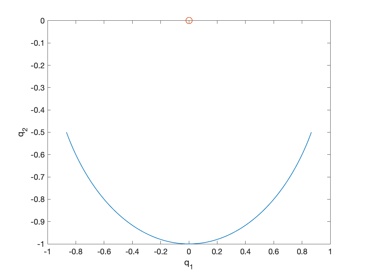
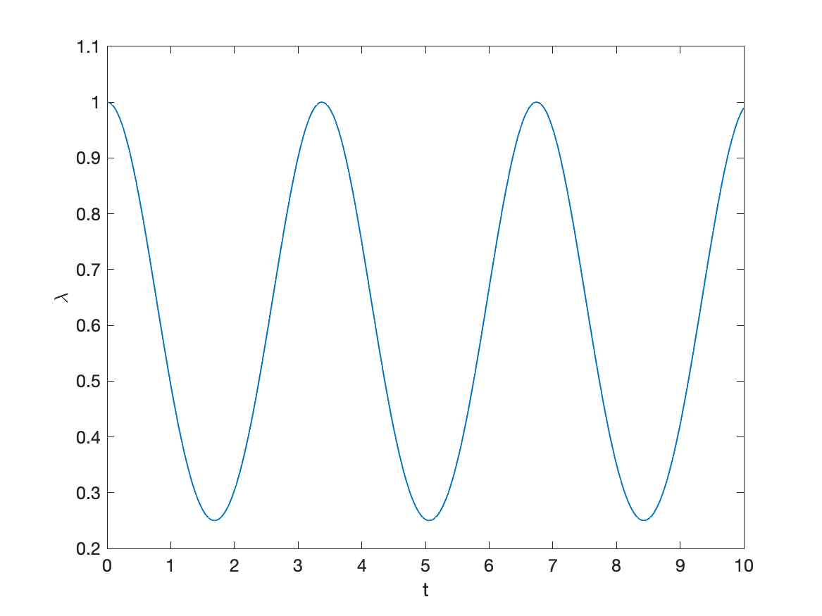
Refer to captionRefer to caption

Figure 1: phase portrait (left) and Lagrange multiplier (right) for problem (118)–(120).

As is well known, in such a case, the Lagrange multiplier has the physical meaning of the tension of the suspension rod. Its plot is in Figure 1, together with the phase portrait of the solution.

5.2 A modified pendulum

Refer to captionRefer to caption

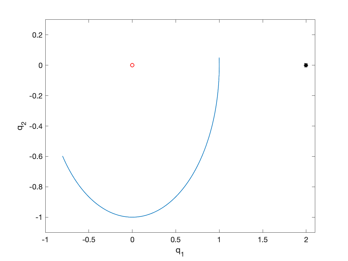
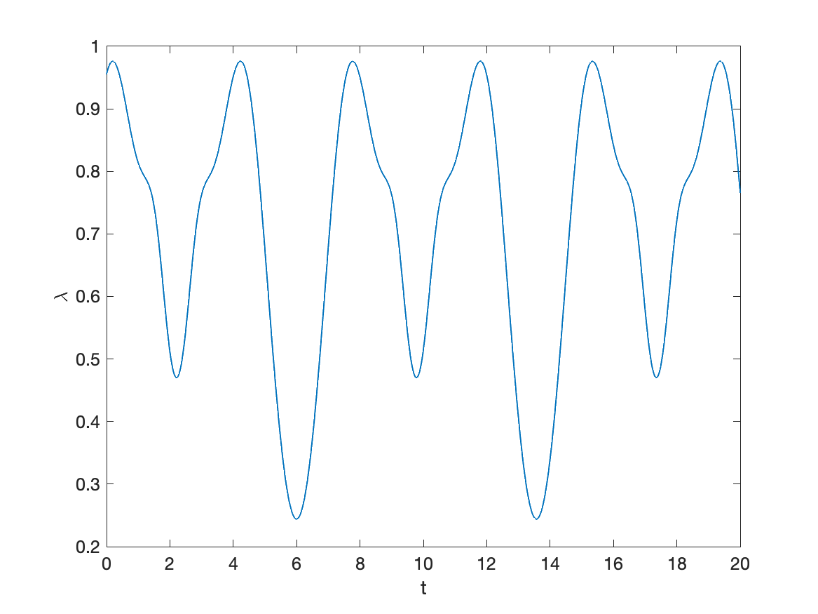
Figure 2: phase portrait (left) and Lagrange multiplier (right) for the problem defined by (122), with q=(2,0)superscript𝑞superscript20topq^{*}=(2,0)^{\top}, using the initial values (120); in the left-plot, the star denotes the second charged point.

In this case, the simple pendulum described in Section 5.1 is modified by assuming that the unit-point mass also has an electric charge. Another charged point is placed at qsuperscript𝑞q^{*}, so that the Hamiltonian becomes:

H(q,p)=12p2+e2q1qq,𝐻𝑞𝑝12superscriptnorm𝑝2superscriptsubscript𝑒2top𝑞1norm𝑞superscript𝑞H(q,p)=\frac{1}{2}\|p\|^{2}+e_{2}^{\top}q-\frac{1}{\|q-q^{*}\|}, (122)

subject to the same constraint in (118). We consider the same initial values (120), and choose q=(2, 0)superscript𝑞superscript2 0topq^{*}=(2,\,0)^{\top}. The corresponding phase portrait and the Lagrange multiplier are depicted in Figure 2, relative to the interval [0,20]020[0,20].

As is clear, the potential is now no more quadratic, so that the HBVM(s,s)𝑠𝑠(s,s) method is no more energy-conserving. Nevertheless, by using a HBVM(k,s)𝑘𝑠(k,s) method, with ks𝑘𝑠k\geq s, the Hamiltonian error should behave as O(h2k)𝑂superscript2𝑘O(h^{2k}), according to Theorem 8. This is confirmed by the numerical results listed in Table 2, obtained by solving the problem on the interval [0,20]020[0,20], with timesteps as defined in (121), by means of the HBVM(k,1)𝑘1(k,1) method, k=1,2,3,4𝑘1234k=1,2,3,4. As one may see, the HBVM(4,1) method is (practically) energy-conserving, for the considered values of the timestep.

Table 2: obtained results for problem (120) and (122) by using HBVM(k,1)𝑘1(k,1) methods with timestep (121). The *** mean that the round-off error level is reached.

k=1𝑘1k=1 i𝑖i eysubscript𝑒𝑦e_{y} rate eλsubscript𝑒𝜆e_{\lambda} rate ehidsubscript𝑒𝑖𝑑e_{hid} rate egsubscript𝑒𝑔e_{g} eHsubscript𝑒𝐻e_{H} rate 3 2.40e-02 3.78e-02 1.25e-03 2.00e-15 9.10e-05 4 5.90e-03 2.0 1.52e-02 1.3 3.12e-04 2.0 1.62e-14 2.28e-05 2.0 5 1.47e-03 2.0 6.54e-03 1.2 7.80e-05 2.0 1.78e-15 5.69e-06 2.0 6 3.67e-04 2.0 3.00e-03 1.1 1.95e-05 2.0 2.89e-15 1.42e-06 2.0 7 9.17e-05 2.0 1.43e-03 1.1 4.87e-06 2.0 5.77e-15 3.56e-07 2.0 k=2𝑘2k=2 i𝑖i eysubscript𝑒𝑦e_{y} rate eλsubscript𝑒𝜆e_{\lambda} rate ehidsubscript𝑒𝑖𝑑e_{hid} rate egsubscript𝑒𝑔e_{g} eHsubscript𝑒𝐻e_{H} rate 3 2.28e-02 3.70e-02 1.25e-03 2.66e-15 8.65e-09 4 5.63e-03 2.0 1.50e-02 1.3 3.12e-04 2.0 1.82e-14 5.41e-10 4.0 5 1.40e-03 2.0 6.49e-03 1.2 7.80e-05 2.0 4.44e-15 3.38e-11 4.0 6 3.50e-04 2.0 2.99e-03 1.1 1.95e-05 2.0 4.11e-15 2.11e-12 4.0 7 8.76e-05 2.0 1.43e-03 1.1 4.87e-06 2.0 3.33e-15 1.25e-13 4.1 k=3𝑘3k=3 i𝑖i eysubscript𝑒𝑦e_{y} rate eλsubscript𝑒𝜆e_{\lambda} rate ehidsubscript𝑒𝑖𝑑e_{hid} rate egsubscript𝑒𝑔e_{g} eHsubscript𝑒𝐻e_{H} rate 3 2.28e-02 3.70e-02 1.25e-03 2.11e-15 7.32e-13 4 5.63e-03 2.0 1.50e-02 1.3 3.12e-04 2.0 5.55e-16 9.77e-15 6.2 5 1.40e-03 2.0 6.49e-03 1.2 7.80e-05 2.0 5.55e-16 5.55e-16 *** 6 3.50e-04 2.0 2.99e-03 1.1 1.95e-05 2.0 7.77e-16 6.66e-16 *** 7 8.76e-05 2.0 1.43e-03 1.1 4.87e-06 2.0 2.89e-15 1.11e-15 *** k=4𝑘4k=4 i𝑖i eysubscript𝑒𝑦e_{y} rate eλsubscript𝑒𝜆e_{\lambda} rate ehidsubscript𝑒𝑖𝑑e_{hid} rate egsubscript𝑒𝑔e_{g} eHsubscript𝑒𝐻e_{H} rate 3 2.28e-02 3.70e-02 1.25e-03 2.22e-16 4.44e-16 4 5.63e-03 2.0 1.50e-02 1.3 3.12e-04 2.0 4.44e-16 4.44e-16 *** 5 1.40e-03 2.0 6.49e-03 1.2 7.80e-05 2.0 4.44e-16 6.66e-16 *** 6 3.50e-04 2.0 2.99e-03 1.1 1.95e-05 2.0 6.66e-16 6.66e-16 *** 7 8.76e-05 2.0 1.43e-03 1.1 4.87e-06 2.0 1.55e-15 1.11e-15 ***

5.3 A conical pendulum

Refer to caption
Figure 3: phase portrait the problem (123)–(125).
Table 3: obtained results for problem (123)–(125) by using HBVM(s,s)𝑠𝑠(s,s) methods with timestep (126). The *** mean that the round-off error level is reached.

s=1𝑠1s=1 i𝑖i eysubscript𝑒𝑦e_{y} rate eλsubscript𝑒𝜆e_{\lambda} ehidsubscript𝑒𝑖𝑑e_{hid} egsubscript𝑒𝑔e_{g} eHsubscript𝑒𝐻e_{H} 0 3.61e-01 3.03e-14 3.33e-16 7.55e-15 2.22e-15 1 1.20e-01 1.6 3.33e-16 1.28e-15 5.55e-16 1.72e-15 2 3.20e-02 1.9 1.67e-15 4.16e-16 7.77e-16 2.22e-16 3 8.11e-03 2.0 1.60e-14 2.33e-15 4.44e-16 1.67e-16 4 2.03e-03 2.0 1.57e-14 1.33e-15 7.77e-16 4.44e-16 s=2𝑠2s=2 i𝑖i eysubscript𝑒𝑦e_{y} rate eλsubscript𝑒𝜆e_{\lambda} ehidsubscript𝑒𝑖𝑑e_{hid} egsubscript𝑒𝑔e_{g} eHsubscript𝑒𝐻e_{H} 0 1.55e-02 1.51e-13 1.11e-15 1.11e-15 6.66e-16 1 1.05e-03 3.9 2.66e-15 1.33e-15 1.33e-15 1.39e-15 2 6.66e-05 4.0 1.07e-14 1.69e-15 2.22e-16 2.78e-16 3 4.18e-06 4.0 1.25e-14 1.44e-15 4.44e-16 3.89e-16 4 2.62e-07 4.0 1.59e-13 4.39e-15 6.66e-16 3.33e-16 s=3𝑠3s=3 i𝑖i eysubscript𝑒𝑦e_{y} rate eλsubscript𝑒𝜆e_{\lambda} ehidsubscript𝑒𝑖𝑑e_{hid} egsubscript𝑒𝑔e_{g} eHsubscript𝑒𝐻e_{H} 0 1.91e-04 2.00e-15 9.44e-16 3.33e-16 1.11e-16 1 3.13e-06 5.9 6.22e-15 9.99e-16 3.33e-16 1.11e-16 2 4.94e-08 6.0 1.18e-14 6.66e-16 5.55e-16 2.22e-16 3 7.74e-10 6.0 2.24e-14 8.88e-16 8.88e-16 2.22e-16 4 1.21e-11 6.0 2.24e-13 2.44e-15 8.88e-16 6.66e-16 s=4𝑠4s=4 i𝑖i eysubscript𝑒𝑦e_{y} rate eλsubscript𝑒𝜆e_{\lambda} ehidsubscript𝑒𝑖𝑑e_{hid} egsubscript𝑒𝑔e_{g} eHsubscript𝑒𝐻e_{H} 0 1.23e-06 1.02e-14 2.75e-15 2.22e-16 4.44e-16 1 4.97e-09 7.9 1.98e-14 6.66e-16 6.66e-16 5.55e-16 2 1.96e-11 8.0 9.18e-14 2.56e-15 4.44e-16 1.11e-16 3 7.69e-14 8.0 1.38e-13 3.08e-15 4.44e-16 2.78e-16 4 8.80e-16 *** 6.98e-14 2.00e-15 4.44e-16 3.89e-16

In this case, the problem is given by:

q˙=p,p˙=e3,g(q):=q21=0,formulae-sequence˙𝑞𝑝formulae-sequence˙𝑝subscript𝑒3assign𝑔𝑞superscriptnorm𝑞210\dot{q}=p,\qquad\dot{p}=-e_{3},\qquad g(q):=\|q\|^{2}-1=0, (123)

e3subscript𝑒3e_{3} being the third unit vector in 3superscript3\mathbb{R}^{3}, with Hamiltonian

H(q,p)=12p2+e3q.𝐻𝑞𝑝12superscriptnorm𝑝2superscriptsubscript𝑒3top𝑞H(q,p)=\frac{1}{2}\|p\|^{2}+e_{3}^{\top}q. (124)

Considering the set of consistent initial conditions:

q(0)=(z00z0),p(0)=(0z00),z0=12,formulae-sequence𝑞0subscript𝑧00subscript𝑧0formulae-sequence𝑝00subscript𝑧00subscript𝑧012q(0)=\left(\begin{array}[]{c}z_{0}\\ 0\\ -z_{0}\end{array}\right),\qquad p(0)=\left(\begin{array}[]{c}0\\ \sqrt{z_{0}}\\ 0\end{array}\right),\qquad z_{0}=\frac{1}{\sqrt{2}}, (125)

the motion lies in the plane q3=z0subscript𝑞3subscript𝑧0q_{3}=-z_{0}, with period T=234π𝑇superscript234𝜋T=2^{\frac{3}{4}}\pi, and the Lagrange multiplier is constant, λ=z0𝜆subscript𝑧0\lambda=z_{0}. The suspension rod then spans a cone, from which the name of the problem (see Figure 3). For this problem, the Lagrange multiplier is exactly computed, so that condition (66) holds true and HBVM(s,s)𝑠𝑠(s,s) methods are expected to be energy-conserving and with order 2s2𝑠2s. This is confirmed by the numerical tests listed in Table 3, obtained by using the timestep

hi=2iT5,i=0,1,,formulae-sequencesubscript𝑖superscript2𝑖𝑇5𝑖01h_{i}=2^{-i}\frac{T}{5},\qquad i=0,1,\dots, (126)

for solving one period. From the results in Table 3, one may see that remarkably enough, also the hidden constraint turns out to be satisfied.

5.4 A tethered satellite system

The last test problem that we consider is a tethered satellite systems of three satellites, forming an equilateral triangle with unit sides, as depicted in Figure 6. Setting

q=(q1q2q3),p=(p1p2p3),qi,pi3,i=1,2,3,formulae-sequence𝑞subscript𝑞1subscript𝑞2subscript𝑞3formulae-sequence𝑝subscript𝑝1subscript𝑝2subscript𝑝3subscript𝑞𝑖formulae-sequencesubscript𝑝𝑖superscript3𝑖123q=\left(\begin{array}[]{c}q_{1}\\ q_{2}\\ q_{3}\end{array}\right),\qquad p=\left(\begin{array}[]{c}p_{1}\\ p_{2}\\ p_{3}\end{array}\right),\qquad q_{i},p_{i}\in\mathbb{R}^{3},\quad i=1,2,3,

we assume the Hamiltonian be given by

H(q,p)=i=13(12pi2+1qi+cos(qi)),𝐻𝑞𝑝superscriptsubscript𝑖1312superscriptnormsubscript𝑝𝑖21normsubscript𝑞𝑖normsubscript𝑞𝑖H(q,p)=\sum_{i=1}^{3}\left(\frac{1}{2}\|p_{i}\|^{2}+\frac{1}{\|q_{i}\|}+\cos(\|q_{i}\|)\right), (127)

with the constraints:

g(q):=(q1q221q2q321q1q321)=03.assign𝑔𝑞superscriptnormsubscript𝑞1subscript𝑞221superscriptnormsubscript𝑞2subscript𝑞321superscriptnormsubscript𝑞1subscript𝑞3210superscript3g(q):=\left(\begin{array}[]{c}\|q_{1}-q_{2}\|^{2}-1\\ \|q_{2}-q_{3}\|^{2}-1\\ \|q_{1}-q_{3}\|^{2}-1\end{array}\right)=0\in\mathbb{R}^{3}. (128)

Consistent initial conditions are chosen as follows:

q1(0)=(012z0),q2(0)=(012z0),q3(0)=(00z032),formulae-sequencesubscript𝑞10012subscript𝑧0formulae-sequencesubscript𝑞20012subscript𝑧0subscript𝑞3000subscript𝑧032q_{1}(0)=\left(\begin{array}[]{c}0\\ \frac{1}{2}\\ z_{0}\end{array}\right),\quad q_{2}(0)=\left(\begin{array}[]{c}0\\ -\frac{1}{2}\\ z_{0}\end{array}\right),\quad q_{3}(0)=\left(\begin{array}[]{c}0\\ 0\\ z_{0}-\frac{\sqrt{3}}{2}\end{array}\right), (129)

and

p1(0)=p2(0)=03,p3(0)=(v000),formulae-sequencesubscript𝑝10subscript𝑝200superscript3subscript𝑝30subscript𝑣000p_{1}(0)=p_{2}(0)=0\in\mathbb{R}^{3},\qquad p_{3}(0)=\left(\begin{array}[]{c}v_{0}\\ 0\\ 0\end{array}\right), (130)

with z0=20subscript𝑧020z_{0}=20 and v0>0subscript𝑣00v_{0}>0 such that H(q(0),p(0))=0𝐻𝑞0𝑝00H(q(0),p(0))=0. Let us numerically solve problem (127)–(130) on the interval [0,103]0superscript103[0,10^{3}] by using the HBVM(1,1) method with timestep h=0.10.1h=0.1. The method is not energy-conserving, and 9.4 sec are required for solving the problem, with a mean number of 15.4 iterations (115) per step. The numerical Hamiltonian is depicted in the left-plot of Figure 6. If we solve the problem by using HBVM(5,1), the method turns out to be practically energy-conserving, and requires 11.6 sec, with the same mean number of iterations (115) per step. The corresponding numerical Hamiltonian is shown in the right-plot of Figure 6. As one may see, the energy-conserving method has a much more appropriate behavior, with a very moderate increase of the computational time.

Refer to caption
Figure 4: tethered satellite system described by problem (127)–(130).

Refer to captionRefer to caption

Figure 5: numerical Hamiltonian when solving problem (127)–(130) with timestep h=0.10.1h=0.1 by using HBVM(1,1) (left plot) and HBVM(5,1) (right plot).

Refer to captionRefer to caption

Figure 6: numerical Hamiltonian when solving problem (127)–(130) with timestep h=0.10.1h=0.1 by using HBVM(3,3) (left plot) and HBVM(5,3) (right plot).

Similar results are obtained by solving the problem, with the same timestep h=0.10.1h=0.1, by using the HBVM(3,3) and HBVM(5,3) methods, the latter method being (practically) energy-conserving. Both methods need a mean of 14 iterations (115) per step, with execution times of 14.2 sec and 15.4 sec, respectively. The corresponding numerical Hamiltonians are depicted in Figure 6. Also in this case, the qualitative results obtained by the energy-conserving method are more favorable, with only a very limited increase of the overall computational cost.

6 Conclusions

In this paper we have introduced a class of energy-conserving methods for Hamiltonian problems with quadratic holonomic constraints. The methods reduce to the class of Hamiltonian Boundary Value Methods (HBVMs), when the constraints are not given. Arbitrarily high-order methods are obtained within this class. A detailed analysis of the methods has been presented, along with their practical implementation and solution of the generated discrete problems. A number of numerical tests duly confirm the theoretical results, also proving the usefulness of the approach. Future directions of investigation will include the extension of the methods for numerically solving Hamiltonian problems with general holonomic constraints.

Conflict of interests.

The authors declare no conflict of interests.

Acknowledgements.

The authors acknowledge the mrSIR project [45] for the financial support.

References

  • [1] H.C. Andersen. Rattle: a “velocity” version of the Shake algorithm for molecular dynamics calculations. J. Comp. Phys. 52 (1983) 24–34.
  • [2] M.F. Baião, T.J. Stuchi. Dynamics of tethered satellites in the vicinity of the Lagrangian point L2subscript𝐿2L_{2} of the Earth-Moon system. Astrophys. Space Sci. 362 (2017) 134
  • [3] G. Benettin, A.M. Cherubini, F. Fassò. A changing chart symplectic algorithm for rigid bodies and other Hamiltonian systems on manifolds. SIAM J. Sci. Comput. 23, No. 4 (2001) 1189–1203.
  • [4] K.E. Brenan, S.L. Campbell, L.R. Petzold. Numerical solution of initial-value problems in differential-algebraic equations. SIAM, Philadelphia, PA, 1996.
  • [5] L. Brugnano, G. Frasca-Caccia, F. Iavernaro. Efficient implementation of Gauss collocation and Hamiltonian Boundary Value Methods. Numer. Algorithms 65 (2014) 633–650.
  • [6] L. Brugnano, G. Gurioli, F. Iavernaro, E. Weinmueller. Line Integral Solution of Hamiltonian Systems with Holonomic Constraints. Appl. Numer. Math. 127 (2018) 56–77.
  • [7] L. Brugnano, F. Iavernaro. Line Integral Methods for Conservative Problems. Chapman et Hall/CRC, Boca Raton, FL, 2016.
  • [8] L. Brugnano, F. Iavernaro. Line Integral Solution of Differential Problems. Axioms 7(2) (2018) 36.
  • [9] L. Brugnano, F. Iavernaro, D. Trigiante. Hamiltonian BVMs (HBVMs): a family of “drift-free” methods for integrating polynomial Hamiltonian systems. AIP Conf. Proc. 1168 (2009) 715–718.
  • [10] L. Brugnano, F. Iavernaro, D. Trigiante. Hamiltonian Boundary Value Methods (Energy Preserving Discrete Line Integral Methods). JNAIAM. J. Numer. Anal. Ind. Appl. Math. 5, No. 1-2 (2010) 17–37.
  • [11] L. Brugnano, F. Iavernaro, D. Trigiante. A note on the efficient implementation of Hamiltonian BVMs. J. Comput. Appl. Math. 236 (2011) 375–383.
  • [12] L. Brugnano, F. Iavernaro, D. Trigiante. A simple framework for the derivation and analysis of effective one-step methods for ODEs. Appl. Math.Comput. 218 (2012) 8475–8485.
  • [13] L. Brugnano, F. Iavernaro, D. Trigiante. Analisys of Hamiltonian Boundary Value Methods (HBVMs): a class of energy-preserving Runge-Kutta methods for the numerical solution of polynomial Hamiltonian systems. Commun. Nonlinear Sci. Numer. Simul. 20 (2015) 650–667.
  • [14] L. Brugnano, C. Magherini. Blended Implementation of Block Implicit Methods for ODEs. Appl. Numer. Math. 42 (2002) 29–45.
  • [15] L. Brugnano, C. Magherini. Recent Advances in Linear Analysis of Convergence for Splittings for Solving ODE problems. Appl. Numer. Math. 59 (2009) 542–557.
  • [16] Z.Q. Cai, X.F. Li, X. F., H. Zhou. Nonlinear dynamics of a rotating triangular tethered satellite formation near libration points. Aerospace Science and Technology 42 (2015) 384–391.
  • [17] P. Console, E. Hairer, C. Lubich. Symmetric multistep methods for constrained Hamiltonian systems. Numer. Math. 124 (2013) 517–539.
  • [18] O. Gonzalez. Mechanical systems subject to holonomic constraints: Differential–algebraic formulations and conservative integration. Physica D 132 (1999) 165–174.
  • [19] E. Hairer. Global modified Hamiltonian for constrained symplectic integrators. Numer. Math. 95 (2003) 325–336.
  • [20] E. Hairer, C. Lubich, G. Wanner. Geometric Numerical Integration, Structure-Preserving Algorithms for Ordinary Differential Equations, Second Edition. Springer-Verlag, Berlin, 2006.
  • [21] E. Hairer, G. Wanner. Solving Ordinary Differential Equations II, Stiff and Differential-Algebraic Problems, Second Revised Edition. Springer-Verlag, Berlin, 2010.
  • [22] E. Hairer, S.P. Nørsett, G. Wanner. Solving Ordinary Differential Equations I, nonstiff problems. Second revised edition (3rd printing). Springer, Heidelberg, 2008.
  • [23] L. Jay. Symplectic partitioned Runge-Kutta methods for constrained Hamiltonian systems. SIAM J. Numer Anal. 33, No. 1 (1996) 368–387.
  • [24] W. Jung, A.P. Mazzoleni, J. Chung. Dynamic analysis of a tethered satellite system with a moving mass. Nonlinear Dyn. 75 (2014) 267–281.
  • [25] W. Jung, A.P. Mazzoleni, J. Chung. Nonlinear dynamic analysis of a three-body tethered satellite system with deployment/retrieval. Nonlinear Dyn. 82 (2015) 1127–1144.
  • [26] D.T. Kawano. On modeling and simulation of tethered systems with sharp, rough contacts Commun. Nonlinear Sci. Numer. Simul. 16 (2011) 550–565.
  • [27] B. Leimkhuler, S. Reich. Symplectic integration of constrained Hamiltonian systems. Math. Comp. 63, No. 208 (1994) 589–605.
  • [28] B. Leimkhuler, S. Reich. Simulating Hamiltonian Dynamics. Cambridge University Press, 2004.
  • [29] B. Leimkhuler, R.D. Skeel. Symplectic numerical integrators in constrained Hamiltonian systems. J. Comput. Phys. 112 (1994) 117–125.
  • [30] S. Leyendecker, P. Betsch, P. Steinmann. Energy-conserving integration of constrained Hamiltonian systems – a comparison of approaches. Computational Mechanics 33 (2004) 174–185.
  • [31] L. Li, D. Wang. Energy and quadratic invariants preserving methods for Hamiltonian systems with holonomic constraints. arXiv:2007.06338 [math.NA].
  • [32] X. Lian, J. Liu, J. Zhang, C. Wang. Chaotic motion and control of a tethered-sailcraft system orbiting an asteroid. Commun. Nonlinear Sci. Numer. Simul. 77 (2019) 203–224.
  • [33] C. Luo, H. Wen, D. Jin, S. Xu. Dynamics of a flexible multi-tethered satellite formation in a Halo orbit with uncertain parameters. Commun. Nonlinear Sci. Numer. Simul. 99 (2021) 105828.
  • [34] S. Reich. Symplectic integration of constrained Hamiltonian systems by composition methods. SIAM J. Numer. Anal. 33 No. 2 (1996) 475–491.
  • [35] S. Reich. On higher-order semi-explicit symplectic partitioned Runge-Kutta methods for constrained Hamiltonian systems. Numer. Math. 76 (1997) 231–247.
  • [36] W.M. Seiler. Position versus momentum projections for constrained Hamiltonian systems. Numer. Algorithms 19 (1998) 223–234.
  • [37] W.M. Seiler. Numerical integration of constrained Hamiltonian systems using Dirac brackets. Math. Comp. 68, No. 226 (1999) 661–681.
  • [38] J.P. Ryckaert, G. Ciccotti, H.J.C. Berendsen. Numerical integration of the cartesian equations of motion of a system with constraints: molecular dynamics of n𝑛n-alkanes. J. Comput. Phys. 23 (1977) 327–341.
  • [39] Y. Wei, Z. Deng, Q. Li, B. Wang. Projected Runge-Kutta methods for constrained Hamiltonian systems. Appl. Math. Mech. – Engl. Ed. 37, No. 8 (2016) 1077–1094.
  • [40] C.Y. Wang, C.M. Wang, R. Freund. Vibration of Heavy String Tethered to Mass-Spring System. Int. J. Struct. Stab. Dyn. 17 (2017) 1771002, 12 pp.
  • [41] M. Xu, J.-M. Zhu, T. Tan, S.-J. Xu. Equilibrium configurations of the tethered three-body formation system and their nonlinear dynamics. Acta Mech. Sin. 28 (2012) 1668–1677.
  • [42] B. Yu, D. Jin, H. Wen. Nonlinear dynamics of flexible tethered satellite system subject to space environment. Appl. Math. Mech. -Engl. Ed. 37(4) (2016) 485–500.
  • [43] Y.M. Zabolotnov. Control of the deployment of a tethered orbital system with a small load into a vertical position. J. Appl. Math. Mech. 79, no. 1 (2015) 28–34.
  • [44] A.E. Zakrzhevskii. Method of deployment of a tethered space system along the local vertical. Internat. Appl. Mech. 51 (2015) 670–681.
  • [45] https://www.mrsir.it/en/