Bandits Corrupted by Nature:
Lower Bounds on Regret and Robust Optimistic Algorithms
Abstract
We study the corrupted bandit problem, i.e. a stochastic multi-armed bandit problem with unknown reward distributions, which are heavy-tailed and corrupted by a history-independent adversary or Nature. To be specific, the reward obtained by playing an arm comes from corresponding heavy-tailed reward distribution with probability and an arbitrary corruption distribution of unbounded support with probability . First, we provide a problem-dependent lower bound on the regret of any corrupted bandit algorithm. The lower bounds indicate that the corrupted bandit problem is harder than the classical stochastic bandit problem with sub-Gaussian or heavy-tail rewards. Following that, we propose a novel UCB-type algorithm for corrupted bandits, namely HuberUCB, that builds on Huber’s estimator for robust mean estimation. Leveraging a novel concentration inequality of Huber’s estimator, we prove that HuberUCB achieves a near-optimal regret upper bound. Since computing Huber’s estimator has quadratic complexity, we further introduce a sequential version of Huber’s estimator that exhibits linear complexity. We leverage this sequential estimator to design SeqHuberUCB that enjoys similar regret guarantees while reducing the computational burden. Finally, we experimentally illustrate the efficiency of HuberUCB and SeqHuberUCB in solving corrupted bandits for different reward distributions and different levels of corruptions.
1 Introduction
Multi-armed bandit problem is an archetypal setting to study sequential decision-making under incomplete information (Lattimore & Szepesvári, 2020). In the classical setting of stochastic multi-armed bandits, the decision maker or agent has access to unknown reward distributions or arms. At every step, the agent plays an arm and obtains a reward. The goal of the agent is to maximize the expected total reward accumulated by a given horizon .
In this paper, we are interested in a challenging extension of the classical multi-armed bandit problem, where the reward at each step is corrupted by Nature, which is a stationary mechanism independent of the agent’s decisions and observations. This setting is often referred as the Corrupted Bandits. Specifically, we extend the existing studies of corrupted bandits (Lykouris et al., 2018; Bogunovic et al., 2020; Kapoor et al., 2019) to the more general case, where the ‘true’ reward distribution might be heavy-tailed (i.e. with a finite number of finite moments) and the corruption can be unbounded.
A Motivating Example: Treatments of Varroa Mites.
Though this article focuses on the theoretical aspects of this problem, we hereby illustrate a case study with roots in agriculture that motivates us. A bee-keeper has to choose between a set of treatments to save her bees from varroa mites. Every year, the bee-keeper must rotate between the treatments as the varroa mites develop resistance to a given treatment (Rinkevich, 2020; Kamler et al., 2016). The goal of the bee-keeper is to choose a sequence of treatments over the years that eliminate as many number of varroa mites as possible. The reward of a treatment is measured by the number of fallen varroa mites due to it. This reward function is heavy-tailed. As the number of fallen varroa mites is counted manually by the bee-keeper, this process is prone to human error.
The corruption in particular has been witnessed empirically while plotting the number of fallen mites for a given treatment (Fig. 1 (Semkiw et al., 2013)). To understand the phenomena of heavy-tailedness and corruption, let us imagine a natural model for the number of dead mites in a given interval of 1 week, i.e. a Poisson distribution (light-tailed distribution). In this case, if the mean of the Poisson distribution is , which is the case in Fig. 1 (Semkiw et al., 2013). Then, the standard deviation of the number of dead mites should be equal to , which contrasts with the standard deviation larger than as reported in the Fig. 1 (Semkiw et al., 2013). Now, it is hard to decouple why this heavy-tailedness suddenly appear, and if there are outliers, what is their distribution or the upper bound on them. Thus, to deal with such observations of reward, we aim to design algorithms that can deal with both heavy-tailedness and unbounded corruptions.
Interestingly, in this problem, corruptions in the measured rewards are natural and non-adversarial but possibly unbounded. The heavy-tailed and corrupted nature of the problem resists application of the non-robust bandit algorithms, such as UCB (Auer et al., 2002a), and motivates us to introduce the setting of Bandits corrupted by Nature.
Bandits corrupted by Nature.
Motivated by the aforementioned example, we model a corrupted reward distribution as , where is the distribution of inliers with a finite variance, is the distributions of outliers with probably unbounded support, and is the proportion of outliers. Thus, in the corresponding stochastic bandit setting, an agent has access to arms of corrupted reward distributions . Here, ’s are uncorrupted reward distributions with heavy-tails and bounded variances, and ’s are corruption distributions with probably unbounded corruptions. The goal of the agent is to maximize the expected total reward accumulated oblivious to the corruptions. This is equivalent to considering a setting where at every step Nature flips a coin with success probability . The agent obtains a corrupted reward if Nature obtains and otherwise, an uncorrupted reward. We call this setting Bandits corrupted by Nature as the corruption introduced in each step does not depend on the present or previous choices of arms and observed rewards. Our setting encompasses both heavy-tailed rewards and unbounded corruptions. We formally define the setting and corresponding regret definition in Section 3.
Bandits corrupted by Nature is different from the adversarial bandit setting (Auer et al., 2002b). The adversarial bandit assumes existence of a non-stochastic adversary that can return at each step the worst-case reward to the agent depending on its history of choices. Incorporating corruptions in this setting, Lykouris et al. (2018); Bogunovic et al. (2020) consider settings where the rewards can be corrupted by a history-dependent adversary but the total amount of corruption and also the corruptions at each step are bounded. However, we encounter problems in ecology and agronomy, such as treatments against varroa mites, where the corruptions are not adversarial, and are independent of the previous history of decisions. Thus, in contrast to the adversarial corruption setting in literature, we consider a non-adversarial proportion of corruptions () at each step, which are stochastically generated from unbounded corruption distributions . To the best of our knowledge, only Kapoor et al. (2019) have studied similar non-adversarial corruption setting with a history-independent proportion of corruption at each step. But they assume that the probable corruptions at each step are bounded, and the uncorrupted rewards are sub-Gaussian. Hence, we observe that there is a gap in the literature in studying unbounded stochastic corruption for bandits with probably heavy-tailed rewards and this article aims to fill this gap. Specifically, we aim to deal with unbounded corruption and heavy-tails simultaneously, which requires us to develop a novel sensitivity analysis of the robust estimator in lieu of a worst-case (adversarial bandits) analysis.
Our Contributions. Specifically, in this paper, we aim to investigate three main questions:
These questions have led us to the following contributions:
1. Hardness of bandits corrupted by Nature with unbounded corruptions and heavy tails. In order to understand the fundamental hardness of the proposed setting, we use a suitable notion of regret, denoted by , (Equation (Corrupted regret), (Kapoor et al., 2019)) that extends the traditional pseudo-regret (Lattimore & Szepesvári, 2020) to the corrupted setting. Then, in Section 4, we derive lower bounds on regret that reveal increased difficulties of corrupted bandits with heavy tails in comparison with the classical non-corrupted and light-tailed Bandits. (a) In the Heavy-tailed regime (3), we show that even when the suboptimality gap 111The suboptimality gap of an arm is the difference in mean rewards of an optimal arm and that arm. is large, the regret increase with because of the difficulty to distinguish between two arms when the rewards of Heavy-tailed. (b) Our lower bounds indicate that when is large, the logarithmic regret is asymptotically achievable, but the hardness depends on the corruption proportion , variance of , i.e. , and the suboptimality gap . Specifically, if ’s are small, i.e. we are in low distinguishability/high variance regime, the hardness is dictated by . Here, is the ‘corrupted suboptimality gap’ that replaces the traditional suboptimality gap in the lower bound of non-corrupted and light-tailed bandits (Lai & Robbins, 1985). Since , it is harder to distinguish the optimal and suboptimal arms in the corrupted settings. They are the same when the corruption proportion .
Additionally, our analysis addresses an open problem in heavy-tailed bandits. Works on heavy-tailed bandits (Bubeck et al., 2013; Agrawal et al., 2021) rely on the assumption that a bound on the -moment, i.e. , is known for some . We do not assume such a restrictive bound as knowing a bound on implies the knowledge of a bound on the sub-optimality gap . Instead, we assume that the centered moment, specifically the variance, is bounded by a known constant. Thus, we address the open problem mentioned in (Agrawal et al., 2021) by relaxing the classical bounded -moment assumption with the bounded centered moment one.
2. Robust and Efficient Algorithm Design. In Section 5, we propose a robust algorithm, called HuberUCB, that leverages the Huber’s estimator for robust mean estimation. We derive a novel concentration inequality on the deviation of empirical Huber’s estimate that allows us to design robust and tight confidence intervals for HuberUCB. In Theorem 3, we show that HuberUCB achieves the logarithmic regret, and also the optimal rate when the sub-optimality gap is not too large. We show that for HuberUCB, can be decomposed according to the respective values of and :
Thus, our upper bound allows us to segregate the errors due to heavy-tail, corruption, and corruption-correction with heavy tails. The error incurred by HuberUCB can be directly compared to the lower bounds obtained in Section 4 and interpreted in both the high distinguishibility regime and the low distinguishibility regime as previously mentioned.
3. Empirically Efficient and Robust Performance. To the best of our knowledge, we present the first robust mean estimator that can be computed in a linear time in a sequential setting (Section 6). Existing robust mean estimators, such as Huber’s estimator, need to be recomputed at each iteration using all the data, which implies a quadratic complexity. Our proposal recomputes Huber’s estimator only when the iteration number is a power of and computes a sequential approximation on the other iterations. We use the Sequential Huber’s estimator to propose SeqHuberUCB. We theoretically show that SeqHuberUCB achieves similar order of regret as HuberUCB, while being computationally efficient. In Section 7, we also experimentally illustrate that HuberUCB and SeqHuberUCB achieve the claimed performances for corrupted Gaussian and Pareto environments.
We further elaborate on the novelty of our results and position them in the existing literature in Section 2. For brevity, we defer the detailed proofs and the parameter tuning to Appendix.
2 Related Work
Due to the generality of our setting, this work either extends or relates to the existing approaches in both the heavy-tailed and corrupted bandits literature. While designing the algorithm, we further leverage the literature of robust mean estimation. In this section, we connect to these three streams of literature. Table 1 summarizes the previous works and posits our work in lieu.
| Algorithms | Settings | Corruption | Type of outliers | Heavy-tailed | Adversarial/ |
|---|---|---|---|---|---|
| Stochastic | |||||
| Our work | MAB | Yes | Unbounded | Yes | Stochastic |
| Bubeck et al. (2013); Agrawal et al. (2021); Lee et al. (2020) | MAB | No | x | Yes | Stochastic |
| Lykouris et al. (2018) | MAB | Yes | Bounded | No | Stochastic |
| Bogunovic et al. (2020) | GP Bandits | Yes | Bounded | No | Adversarial |
| Kapoor et al. (2019) | MAB & Linear Bandits | Yes | Bounded | No | Stochastic |
| Medina & Yang (2016); Shao et al. (2018) | Linear Bandits | No | x | Yes | Stochastic |
| Bouneffouf (2021) | Contextual Bandits | context only | Unbounded | No | Stochastic |
| Agarwal et al. (2019) | Control | Yes | Bounded | x | Adversarial |
| Hajiesmaili et al. (2020); Auer et al. (2002b); Pogodin & Lattimore (2020) | MAB | Yes | Bounded | x | Adversarial |
Heavy-tailed bandits. Bubeck et al. (2013) are one of the first to study robustness in multi-armed bandits by studying the heavy-tailed rewards. They use robust mean estimator to propose the RobustUCB algorithms. They show that under assumptions on the raw moments of the reward distributions, a logarithmic regret is achievable. It sprouted research works leading to either tighter rates of convergence (Lee et al., 2020; Agrawal et al., 2021), or algorithms for structured environments (Medina & Yang, 2016; Shao et al., 2018). Our article uses Huber’s estimator which was already discussed in (Bubeck et al., 2013). However, the chosen parameters in (Bubeck et al., 2013) were suited for heavy-tailed distributions, and thus, render their proposed estimator non-robust to corruption. We address this gap in this work.
Corrupted bandits. The existing works on Corrupted Bandits (Lykouris et al., 2018; Bogunovic et al., 2020; Kapoor et al., 2019) are restricted to bounded corruption. When dealing with bounded corruption, one can use techniques similar to adversarial bandits Auer et al. (2002b) to deal with an adversary that can’t corrupt an arm too much. The algorithms and proof techniques are fundamentally different in our article because the stochastic (or non-adversarial) corruption by Nature allows us to learn about the inlier distribution on the condition that corresponding estimators are robust. Thus, our bounds retain the problem-dependent regret, while successfully handling probably unbounded corruptions with robust estimators.
Robust mean estimation. Our algorithm design leverages the rich literature of robust mean estimation, specifically the influence function representation of Huber’s estimator. The problem of robust mean estimation in a corrupted and heavy-tailed setting stems from the work of Huber (Huber, 1964; 2004). Recently, in tandem with machine learning, there have been numerous advances both in the heavy-tailed (Devroye et al., 2016; Catoni, 2012; Minsker, 2019), and in the corrupted settings (Lecué & Lerasle, 2020; Minsker & Ndaoud, 2021; Prasad et al., 2019; 2020; Depersin & Lecué, 2019; Lerasle et al., 2019; Lecué & Lerasle, 2020). Our work, specifically the novel concentration inequality for Huber’s estimator, enriches this line of work with a result of parallel interest. We introduce a sequential version of Huber’s estimator achieving linear complexity.
3 Bandits corrupted by Nature: Problem formulation
In this section, we present the corrupted bandits setting that we study, together with the corresponding notion of regret. Similarly to the classical bandit setup, the regret decomposition lemma allows us to focus on the expected number of pulls of a suboptimal arm as the central quantity to control algorithmic standpoint.
Notations. We denote by the set of probability distributions on the real line and by the set of distributions with at least finite moments. is the indicator function for the event being true. We denote the mean of a distribution as . For any , we denote the set of corrupted distributions from .
Problem Formulation.
In the setting of Bandits corrupted by Nature, a bandit algorithm faces an environment with many reward distributions in the form . Here are real-valued distributions and is a mixture parameter assumed to be in , that is is given more weights than in the mixture of arm . For this reason the are called the inlier distributions and the the outlier distributions. We assume the inlier distributions have at least finite moments that is , while no restriction is put on the outlier distributions, that is . For this reason, we also refer to the outlier distributions as the corrupted distributions, and to the inlier distributions as the non-corrupted ones. is called the level of corruption. We write the law of the corrupted environment, and we refer to that of the non-corrupted environment by .
The game proceed as follows: At each step , the agent policy interacts with the corrupted environment by choosing an arm and obtaining a reward corrupted by Nature. To generate this reward, Nature first draws a random variable from a Bernoulli distribution with mean . If , it generates a corrupted reward from distribution corresponding to the chosen arm . Otherwise, it generates a non-corrupted from distribution . More formally, Nature generates reward which the learner observes. The learner leverages this observation to choose another arm at the next step in order to maximize the total cumulative reward obtained after steps. In Algorithm 1, we outline a pseudocode of this framework.
Remark 1 (Non-adversarial corruption.)
In the setting of Bandits corrupted by Nature, we consider that the reward received by the learner is corrupted when and non-corrupted otherwise. Since the law of is a Bernoulli , the corruption is stochastic, and independent on other variables. This is in contrast with adversarial setups, where corruption is typically chosen by an opponent and possibly depending on other variables. Assuming a non-adversarial behavior of the Nature seem more justified than assuming an adversarial setup in applications, such as agriculture where corruption is often due to external disturbances, such as pests appearance or weather hazards, whose occurrence are typically non-adversarial. Now when corruption happens, we do not put restriction on the level of corruption. For example, we can imagine a pest outburst or hail, that may have huge impact on a crop but does not occur adversarially.
Remark 2 (Weak assumption on inliers)
Let us highlight that we do not assume sub-Gaussian behavior for the inlier distributions . Instead, we consider only a weak moment assumption, i.e. the inlier distributions have a finite variance. Thus, our setting is capable of modeling both the heavy-tailed and corrupted settings. We highlight this generality in the regret lower bounds and empirical performance analysis in Section 4 and 7.
Corrupted regret.
In this setting, we observe that a corrupted reward distribution () might not have finite mean, unlike the true ’s. Thus, the regret with respect to the corrupted reward distributions might fail to quantify the goodness of the policy and its immunity to corruption while learning.
In this setup, the natural notion of expected regret is measured with respect to the mean of the non-corrupted environment specified by . We define the regret of learning algorithm playing strategy after steps of interaction with the environment as
| (Corrupted regret) |
The expectation is crucially taken on and but not on and . The expectation on the right also incorporates possible randomization from the learner. Thus, (Corrupted regret) quantifies the loss in the rewards accumulated by policy from the inliers while learning only from the corrupted rewards and also not knowing the arm with the best true reward distribution. Thus, this definition of corrupted regret quantifies the rate of learning of a bandit algorithm as regret does for non-corrupted bandits. A similar notion of regret is considered in (Kapoor et al., 2019) that deals with bounded stochastic corruptions.
Due to the non-adversarial nature of the corruption, the regret can be decomposed, as in classical stochastic bandits, to make appear the expected number of pulls of suboptimal arms , which allow us to focus the regret analysis on bounding these terms.
Lemma 1 (Decomposition of corrupted regret)
In a corrupted environment , the regret writes
where denotes the number of pulls of arm until time and the problem-dependent quantity is called the suboptimality gap of arm .
4 Lower bounds for uniformly good policies under heavy-tails and corruptions
In order to derive the lower bounds, it is classical to consider uniformly good policies on some family of environments, Lai & Robbins (1985). We introduce below the corresponding notion for corrupted environments with the set of laws , where for each .
Definition 1 (Robust uniformly good policies)
Let be a family of corrupted bandit environments on . For a corrupted environment with corresponding uncorrupted environment , let denote the mean reward of arm in the uncorrupted setting and denote the maximum mean reward. A policy is uniformly good on if for any ,
Since the corrupted setup is a special case of stochastic bandits, a lower bound can be immediately recovered with classical results, such as Lemma 2 below, that is a version of the change of measure argument (Burnetas & Katehakis, 1997), and can be found in (Maillard, 2019, Lemma 3.4).
Lemma 2 (Lower bound for uniformly good policies)
Let , where for each and let . Then, any uniformly good policy on must pull arms such that for any , ,
where .
Lemma 2 is used in the traditional bandit literature to obtain lower bound on the regret using the decomposition of regret from Lemma 1. In our setting however, the lower bound is more complex as it involves optimization on the non-convex set of distributions with a bounded variance. It also involves an optimization in both the first and second term of the KL because we consider the worst-case corruption in both the optimal arm and non-optimal arm . In this section, we do not solve these problems, but we propose lower bounds derived from the study of a specific class of heavy-tailed distributions on one hand (Lemma 3) and the study of a specific class of corrupted (but not heavy-tailed) distributions on the other hand (Lemma 4).
Using the fact that is an infimum that is smaller than the for the choice , Lemma 2 induces the following weaker lower-bound:
| (1) |
Equation (1) shows that it is sufficient to have an upper bound on the -divergence of the reward distributions interacting with the policy to get a lower bound on the number of pulls of a sub-optimal arm.
In order to bound the -divergence, we separately focus on two families of reward distributions, namely Student’s distribution without corruption and corrupted Bernoulli distribution, that reflect the hardness due to heavy-tails and corruptions, respectively.
Student’s distribution without corruption.
To obtain a lower bound in the heavy-tailed case we use Student distributions. Student distribution are well adapted because they exhibit a finite number of finite moment which makes them heavy-tailed, and we can easily change the mean and variances of Student distribution without changing its shape parameter . We denote by the set of Student distributions with degrees of freedom,
Lemma 3 (Control of KL-divergence for Heavy-tails)
Let be two Student distributions with degrees of freedom with and . Then,
| (2) |
Corrupted Bernoulli distributions.
Now, we study the cost of corruption using the corrupted Bernoulli distributions. Let be two Bernoulli distributions on such that . We corrupt both and with a proportion to get and . We obtain Lemma 4 that illustrates three bounds on as functions of the sub-optimality gap , variance , and corruption proportion .
Lemma 4 (Control of KL-divergence for Corruptions)
There exists two Bernoulli probability distribution with and for which there exists and some -corruptions of and respectively, that have shifted sub-optimality gap given by . Furthermore, they can be chosen so as to satisfy
Uniform Bound. For any , we have
| (3) |
High Distinguishability/Low Variance Regime. If , we get
| (4) |
Low Distinguishability/High Variance Regime. If , there exists and some - versions of and such that .
Consequences of Lemma 4. We illustrate the bounds of Lemma 4 in Figure 1. The three upper bounds on the KL-divergence of corrupted Bernoullis provide us some insights regarding the impact of corruption.
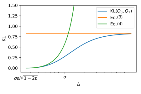
1. Three Regimes of Corruption: We observe that depending on , we can categorize the corrupted environment in three categories. For , we observe that the KL-divergence between corrupted distributions and is upper bounded by a function of only corruption proportion and is independent of the uncorrupted distributions. Whereas for , the distinguishability of corrupted distributions depend on the distinguishibility of uncorrupted distributions and also the corruption level. We call this the High Distinguishability/Low Variance Regime. For , we observe that the KL-divergence can always go to zero. We refer to this setting as the Low Distinguishability/High Variance Regime.
2. High Distinguishability/Low Variance Regime: In Lemma 4, we observe that the effective gap to distinguish the optimal arm to the closest sub-optimal arm that dictates hardness of a bandit instance has shifted from the uncorrupted gap to a corrupted suboptimality gap: .
3. Low Distinguishability/High Variance Regime: We notice also that there is a limit for below which the corruption can make the two distributions and indistinguishable, this is a general phenomenon in the setting of testing in corruption neighborhoods (Huber, 1965).
From KL Upper bounds to Regret Lower Bounds. Substituting the results of Lemma 3 and 4 in Equation (1) yield the lower bounds on regret of any uniformly good policy in heavy-tailed and corrupted settings, where reward distributions either belong to the class of corrupted student distributions or the class of corrupted Bernoulli distributions, respectively. We denote
where is the set of Student distributions with more than degrees of freedoms. We also define
where is the set of corrupted Bernoulli distributions.
Theorem 1 (Lower bound for heavy-tailed and corrupted bandit)
Let be a suboptimal arm such that and denote and .
Student’s distributions. Suppose that the arms are pulled according to a policy that is uniformly good on . Then,
| (5) |
Corrupted Bernoulli distributions: Suppose that the arms are pulled according to a policy that is uniformly good on . Then, we have for , then
| (6) |
and for ,
| (7) |
For brevity, the detailed proof is deferred to Appendix A.1.
Small gap versus large gap regimes.
Due to the restriction in the family of distributions considered in Theorem 1, the lower bounds are not tight and may not exhibit the correct rate of convergence for all families of distributions. However, this theorem provide some insights about the difficulties that one may encounter in corrupted and heavy-tail bandits problems, including the logarithmic dependence on .
In Theorem 1, if is small, we see that in the heavy-tailed case (Student’s distribution), we recover a term very similar to the lower bound when the arms are from a Gaussian distribution. Now in the case where is large, the number of suboptimal pulls in the heavy-tail setting is . This is the price to pay for heavy-tails.
If we are in the high distiguishability/low variance regime, i.e. , we recover a logarithmic lower bound which depends on a corrupted gap between means . Since the corrupted gap is always smaller than the true gap , this indicates that a corrupted bandit () must incur higher regret than a uncorrupted one (). For , this lower bound coincides with the lower bound for Gaussians with uncorrupted gap of means and variance . On the other hand, if is larger than , we observe that we can still achieve logarithmic regret but the hardness depends on only the corruption level , specifically .
5 Robust bandit algorithm: Huber’s estimator and upper bound on the regret
In this section, we propose an UCB-type algorithm, namely HuberUCB, addressing the Bandits corrupted by Nature setting (Algorithm 2). This algorithm uses primarily a robust mean estimator called Huber’s estimator (Section 5.1) and corresponding confidence bound to develop HuberUCB (Section 5.2). We further provide a theoretical analysis in Theorem 3 leading to upper bound on regret of HuberUCB. We observe that the proposed upper bound matches the lower bound in Theorem 1 under some settings.
5.1 Robust mean estimation and Huber’s estimator
We begin with a presentation of the Huber’s estimator of mean (Huber, 1964).
As we aim to design a UCB-type algorithm, the main focus is to obtain an empirical estimate of the mean rewards. Since the rewards are heavy-tailed and corrupted in this setting, we have to use a robust estimator of mean. We choose to use Huber’s estimator (Huber, 1964), an M-estimator that is known for its robustness properties and have been extensively studied (e.g. the concentration properties (Catoni, 2012)).
Huber’s estimator is an M-estimator, which means that it can be derived as a minimizer of some loss function. Given access to i.i.d. random variables , we define Huber’s estimator as
| (8) |
where is Huber’s loss function with parameter . is a loss function that is quadratic near and linear near infinity, with thresholding between the quadratic and linear behaviors.
In the rest of the paper, rather than using the aforementioned definition, we represent the Huber’s estimator as a root of the following equation (Mathieu, 2021):
| (9) |
Here, is called the influence function. Though the representations in Equation (8) and (9) are equivalent, we prefer to use representation Equation (9) as we prove the properties of Huber’s estimator using those of .
plays the role of a scaling parameter. Depending on , Huber’s estimator exhibits a trade-off between the efficiency of the minimizer of the square loss, i.e. the empirical mean, and the robustness of the minimizer of the absolute loss, i.e. the empirical median.
5.2 Concentration of Huber’s estimator in corrupted setting
Let use denote the true Huber mean for a distribution as . This means that for a random variable with law , satisfies .
We now state our first key result on the concentration of Huber’s estimator around in a corrupted and Heavy-tailed setting.
Theorem 2 (Concentration of Empirical Huber’s estimator)
Suppose that are i.i.d. with law for some and proportion of outliers , and has a finite variance . Then, with probability larger than ,
Here, with , , , and
Theorem 2 gives us the concentration of around , i.e. the Huber functional of the inlier distribution . This theorem will allow us to construct a UCB-type algorithm to solve the Bandits corrupted by Nature.
For convenience of notation, hereafter, we denote the rate of convergence of to as
| (10) |
Discussion. Now, we provide a brief discussion on the implications of Theorem 2.
1. Value of : For most laws that exhibit concentration properties, the constant is close to as . One might also use Markov inequality to lower bound , depending on the number of finite moments has. Bounding then becomes a trade-off on the value of , where large values of implies that is close to . But larger also leads to a less robust estimator, since the error bound in Theorem 2 increases with .
2. Tightness of constants: If there are no outliers (), the optimal rate of convergence in such a setting is at least of order due to the central limit theorem. Theorem 2 shows that we are very close to attaining this optimal constant in the leading term. This result for Huber’s estimator echoes the one presented in (Catoni, 2012).
3. Value of : is a parameter that achieve a trade-off between accuracy in the light-tailed uncorrupted setting and robustness. For our result, must be at least of the order of . We provide a detailed discussion on the choice of in Section 5.4.
4. Restriction on the values of : In Theorem 2, must be at least of order . This restriction may seem arbitrary but it is in fact unavoidable as shown in (Devroye et al., 2016, Theorem 4.3). This is a limitation of robust mean estimation that enforces our algorithm to perform a forced exploration in the beginning.
5. Restriction on the values of : In Theorem 2, can be at most , which implies that it is smaller than . This restriction is common in robustness literature. In particular, in Kapoor et al. (2019), is supposed smaller than . In robustness literature, Lecué & Lerasle (2020) and Dalalyan & Thompson (2019) assumed that and respectively. In contrast, our analysis can handle up to , which is significantly higher than the existing restrictions.
Bias of Huber’s Estimate.
If is symmetric, we have . When is non-symmetric, we need to control the distance of the Huber’s estimate from the true mean, i.e. . We call it the bias of Huber’s estimate. We need to bound this bias to get a concentration of the empirical Huber’s estimate around the true mean . We control the bias using the following lemma, which is a direct consequence of (Mathieu, 2021, Lemma 4).
Lemma 5 (Bias of Huber’s estimator)
Let be a random variable with for and suppose that . Then
5.3 HuberUCB: Algorithm and regret bound
In this section, we describe a robust, UCB-type algorithm called HuberUCB. We denote as the mean of arm and its variance as . We assume that we know the variances of the reward distributions. We refer to Section 5.4 for a discussion on the choice of the parameters when the reward distributions are unknown.
HuberUCB: The algorithm.
In order to deploy the Huber’s estimator in the multi-armed bandits setting, we need to estimate the mean of the rewards of each arm separately. We do that by defining a parameter for each arm and estimating separately each using
Now, at each step , we define a confidence bound for arm with number of pulls as
| (11) |
where is defined by Equation (10), , , and is a bound on the bias . is zero if is symmetric and controlled by Lemma 5 otherwise. For example, one can assign by imposing , i.e. finite second moment, in Lemma 5.
Now, we propose HuberUCB that selects an arm at step based on the index
| (12) |
The index of HuberUCB together with the confidence bound defined in Equation (11) dictates that if an arm is less explored, i.e. , we choose that arm, and if multiple arms satisfy this, we break the tie randomly. As grows and for all the arms is satisfied, we choose the arms according to the adaptive bonus. Thus, HuberUCB induces an initial forced exploration to obtain confident-enough robust estimates followed by a time-adaptive selection of arms. We present a pseudocode of HuberUCB in Algorithm 2.
Regret Analysis. Now, we provide a regret upper bound for HuberUCB.
Theorem 3 (Upper Bound on number of pulls of suboptimal arms with HuberUCB)
Suppose that for all , we have , i.e. a reward distribution with finite variance . We assign and such that and . We denote and .
If , then
If , then
We now state a simplified version of Theorem 3 with worse but explicit constants for easier comprehension. Let us fix and such that , and . Now, if we further assume that symmetric leading to , it yields the following upper bounds.
Corollary 1 (Simplified version of Theorem 3)
Suppose that for all , is a symmetric distribution with finite variance . Let also denote for .
If , then
If , then
Remark that in this corollary, we replaced some occurrences of by its upper bound, which is also an upper bound on . Thus, the presented result is loose up to constants but lend itself to easier comprehension.
Discussions on the Upper Bound.
Here, we discuss how this proposed upper bound of HuberUCB matches and mismatches with the lower bounds in Theorem 1.
1. Order-optimality of Upper Bound. HuberUCB achieves the logarithmic regret prescribed by the lower bound (Theorem 1) plus some additive error due to the fact that this is a UCB-type algorithm. Thus, HuberUCB is order optimal with respect to .
2. Two Regimes of Upper Bound. When is small compared to , we obtain an upper bound from Corollary 1. is of the same order of magnitude as Equation (7) because we take strictly smaller than . acts as an indicator of the corruption level. The term indicates the hardness due to the corrupted gaps and echoes the hardness term that appears in regret upper bound of UCB for uncorrupted bandits. The hardness term also appears in the corrupted lower bound (Equation (6)) as well as the heavy-tailed lower bound (Equation (5)) for 222We observe that the lower bound in Equation (5) depends on for , since the first order approximation of is as ..
On the other hand, if is larger than , we get that . This upper bound reflects the lower bound in Equation (7) that holds for . This reinstates the fact that for large enough suboptimality gaps, the regret of HuberUCB depends solely on the corruption level than the suboptimality gap.
3. Deviation from the Lower Bound. The two regimes defined in the upper bound does not follow the exact distinctions made in the lower bounds. We observe that in upper bound, the distinction between regimes depend on a shifted suboptimality gap , while the lower bound depends on the corrupted suboptimality gap . This difference in constants hinder the hardness regimes and corresponding constants in upper and lower bounds to match for all and . This deviation also comes from the fact that the lower bounds proposed in Theorem 1 consider effects of heavy-tails and corruptions separately, while the upper bound of HuberUCB consider them in a coupled manner.
Additionally, we observe that regret of HuberUCB is suboptimal due to the constant additive error, which appears due to the initial forced exploration of HuberUCB up to . Our concentration bounds and corresponding regret analysis shows that this forced exploration phase is unavoidable in order to be able to handle the case with HuberUCB. Removing this discrepancy between the lower and upper bounds would constitute an interesting future work.
5.4 Computational Details
Here, we discuss the three hyperparameters that HuberUCB depends on and also its computational cost.
Choice of and . In Theorem 3, we assume to know the and . In practice, these are unknown and we estimate with a robust estimator of the variance, such as the median absolute deviation. In contrast, estimating is hard. There exists some heuristics, for example using proportion of point larger than 1.5 times the inter-quartile range or using more complex algorithms like Isolation Forest algorithm but these methods work in general using the hypothesis that outliers are in some way points that are located outside of “the bulk of the data" which conflicts with the fact that we don’t suppose anything on the outliers. Moreover even though there are heuristics, the problem of finding what constitute “the bulk of the data" is closely linked to problems such as finding a “Robust minimum volume ellipsoid" which is NP-hard in general (Mittal & Hanasusanto, 2022). We refer to Appendix C.1 for an ablation study on the choice of .
Choice of . Ideally, should be larger than . We recommend using the estimator of to estimate a good value of . The choice of reflects the difference between heavy-tailed bandits and corrupted bandits. When the data are heavy-tailed but not corrupted, Catoni (2012) shows that is a good choice for the scaling parameter. However, this choice is not robust to outliers and yields a linear regret in our setup (see Section 7). When there is corruption, must remains bounded even when the sample size goes to infinity in order to retain robustness. In Appendix C.1, we present an ablation study on the choice of .
Computational Cost. Huber’s estimator has linear complexity due to the involved Iterated Re-weighting Least Squares algorithm, which is not sequential. We have to do this at every iteration, which leads HuberUCB to have a quadratic time complexity. This is the computational cost of using a robust mean estimator, i.e. the Huber’s estimator.
6 SeqHuberUCB: A Faster Robust Bandit Algorithm
In this section, we present a sequential approximation of the Huber’s estimator, and we leverage it further to create a robust bandit algorithm with linear-time complexity algorithm. Here, we describe the algorithm (SeqHuberUCB) and its theoretical properties.
A sequential approximation of Huber’s estimator.
The central idea is to compute the Huber’s estimator using the full historical data only in logarithmic number of steps than at every step, and in between two of these re-computations, update the estimator using only the samples observed at that step. This allows us to propose a sequential approximation of Huber’s estimator, i.e. , with lower computational complexity.
By fixing the update step before a given step , we define the estimator by and
| (13) |
Here, and is the influence function defined in Equation (9). can be conceptualized as a first order Taylor approximation of around .
One might argue that is not fully sequential rather a phased estimator as we still recompute the Huber’s estimator following a geometric schedule. Thus, we still need to keep all the data in memory, leading to linear space complexity as the non-sequential Huber’s estimator. But it features the good property of having a linear time complexity when computed using the prescribed geometric schedule. This implies that the SeqHuberUCB algorithm leveraging the sequential Huber’s estimator achieves a linear time complexity.
Concentration Properties of . Now, in order to propose SeqHuberUCB we first aim to derive the rate of convergence of towards the true Huber’s mean .
Theorem 4
We observe that the confidence bound of includes the confidence bound of , i.e. , and an additive term proportional to . Since for , we can show that . Thus, we obtain larger confidence bounds for than that of , and they differ approximately by a multiplicative constant as .
SeqHuberUCB: The algorithm.
Now, we plug-in the sequential Huber’s estimator, , and the corresponding confidence bound (Equation (14)), instead of the Huber’s estimator and the corresponding confidence bound in the HuberUCB algorithm. This allows us to construct the SeqHuberUCB algorithm that we present hereafter.
Specifically, we define the index of SeqHuberUCB as
| (15) |
where
and a confidence bound for arm with number of pulls is
Here, , and are same as defined for HuberUCB.
Similar to Corollary 1, we now present a simplified regret upper bound for SeqHuberUCB. Retaining the setting of Corollary 1, we assume that , implying , , and symmetric so that . Further simplifying the constants yields the following regret upper bound for SeqHuberUCB.
Lemma 6 (Simplified Upper Bound on Regret of SeqHuberUCB)
Suppose that for all , is a distribution with finite variance . Let us also denote ,
If , then
If , then
Comparison between Regrets of HuberUCB and SeqHuberUCB. Lemma 6 yields similar regret bounds for SeqHuberUCB as the ones obtained for HuberUCB in Corollary 1. We observe that the regrets of these two algorithms only differ in -independent constants. Specifically, regret of SeqHuberUCB can be approximately times higher than that of HuberUCB. For simplicity of exposition, we present approximate constants in our results. A more careful analysis might yield more fine-tuned constants. Theorem 4 and experimental results (Figure 2) indicate that it is possible to have very close performances with SeqHuberUCB and HuberUCB.
7 Experimental Evaluation
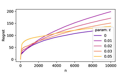
In this section, we assess the experimental efficiency of HuberUCB and SeqHuberUCB by plotting the empirical regret. Contrary to the uncorrupted case, we cannot really estimate the corrupted regret in (Corrupted regret) only using the observed rewards. Instead, we use the true uncorrupted gaps that we know because we are in a simulated environment, and we estimate the corrupted regret using , where is a Monte-Carlo estimation of over experiments. We use rlberry library (Domingues et al., 2021) and Python3 for the experiments. We run the experiments on an 8 core Intel(R) Core(TM) i7-8665U CPU@1.90GHz. For each algorithm, we perform each experiment times to get a Monte-Carlo estimate of regret.
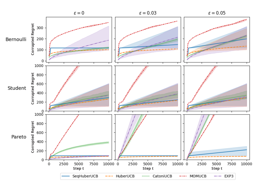
Comparison with Bandit Algorithms for Heavy-tailed and Adversarial Settings. To the best of our knowledge, there is no existing bandit algorithm for handling unbounded stochastic corruption prior to this work. Hence, we focus on comparing ourselves to the closest settings, i.e. bandits in heavy-tailed setting and adversarial bandit algorithms. We empirically and competitively study five different algorithms: HuberUCB, SeqHuberUCB, two RobustUCB algorithms with Catoni-Huber estimator and Median of Means (MOM) (Bubeck et al., 2013), and and adversarial bandit algorithm: Exp3.
HuberUCB is closely related to the RobustUCB with Catoni Huber estimator, which also uses Huber’s estimator but with another set of parameters and confidence intervals. The RobustUCB algorithms are tuned for uncorrupted heavy-tails. Hence, they incur linear regret in a corrupted setting. This is reflected in the experiments. We also improve upon (Bubeck et al., 2013) as we can handle arm-dependent variances. Exp3 is an algorithm designed for bounded Adversarial corruption, and thus, fails as the corruption is too severe.
Corrupted Bernoulli setting: In Figure 2 (above), we study a 3-armed bandits with corrupted Bernoulli distributions with means . The corruption applied to this bandit problem are Bernoulli distributions with means , respectively. For HuberUCB and SeqHuberUCB, we choose to use , which seems to work better despite the theory presented before. We plot the mean plus/minus the standard error of the result in Figure 2. We do that for the three corruption proportions equal to , and . We notice that there is a short linear regret phase at the beginning due to the forced exploration performed by the algorithms. Followed by that, HuberUCB and SeqHuberUCB incur logarithmic regret. On the other hand, Exp3, Catoni Huber Agent and MOM Agent incur logarithmic regret only in the uncorrupted setting. When the data are corrupted, i.e. , their regret grow linearly.
Corrupted Student setting: In Figure 2 (middle), we study a 3-armed bandits with corrupted Student’s distributions with degrees of freedom (finite second moment) and with means . The corruption applied to this bandit problem are Gaussians with variance , and means respectively. For HuberUCB and SeqHuberUCB, we choose to use . The results echo the observations for the Bernoulli case except that the corruption is more drastic and affect the performance even more.
Corrupted Pareto setting: In Figure 2 (bottom), we illustrate the results for a 3-armed bandits with corrupted Pareto distributions having shape parameters (i.e. they have finite second moments), and scale parameters respectively. Thus, the corresponding means are and and the standard deviations are , respectively. The corruption applied to this bandit problem are Gaussians with variance , and centered at respectively. For HuberUCB and SeqHuberUCB, we choose to use and we also bound the bias by . The results echo the observations for the Student’s distributions.
Thus, we conclude that HuberUCB incur the lowest regret among the competing algorithms in the Bandits Corrupted by Nature setting, specially for higher corruption levels . Also, performances of SeqHuberUCB and HuberUCB are very close except for the Pareto distributions with high corruption level.
8 Conclusion
In this paper, we study the setting of Bandits corrupted by Nature that encompasses both the heavy-tailed rewards with bounded variance and unbounded corruptions in rewards. In this setting, we prove lower bounds on the regret that shows the heavy-tail bandits and corrupted bandits are strictly harder than the usual sub-Gaussian bandits. Specifically, in this setting, the hardness depends on the suboptimality gap/variance regimes. If the suboptimality gap is small, the hardness is dictated by . Here, is the corrupted sub-optimality gap, which is smaller than the uncorrupted gap and thus, harder to distinguish. To complement the lower bounds, we design a robust algorithm HuberUCB that uses Huber’s estimator for robust mean estimation and a novel concentration bound on this estimator to create tight confidence intervals. HuberUCB achieves logarithmic regret that matches the lower bound for low suboptimality gap/high variance regime. We also present a sequential Huber estimator that could be of independent interest and we use it to state a linear-time robust bandit algorithm, SeqHuberUCB, that presents the same efficiency as HuberUCB. Unlike existing literature, we do not need any assumption on a known bound on corruption and a known bound on the -uncentered moment, which was posed as an open problem in (Agrawal et al., 2021).
Since our upper and lower bounds disagree in the high gap/low variance regime, it will be interesting to investigate this regime further. From multi-armed bandits, we know that the tightest lower and upper bounds depend on the KL-divergence between optimal and suboptimal reward distributions. Thus, it would be imperative to study KL-divergence with corrupted distributions to better understand the Bandits corrupted by Nature problem. In this paper, we have focused on a problem-dependent regret analysis for a given . In future, it would be interesting to get some insight on how to adapt to an unknown , and to perform a problem-independent “worst-case" analysis. Also, following the reinforcement learning literature, it will be natural to extend HuberUCB to contextual and linear bandit settings with corruptions and heavy-tails. This will facilitate its applicability to practical problems, such as choosing treatments against pests.
References
- Agarwal et al. (2019) Naman Agarwal, Brian Bullins, Elad Hazan, Sham Kakade, and Karan Singh. Online control with adversarial disturbances. In Kamalika Chaudhuri and Ruslan Salakhutdinov (eds.), Proceedings of the 36th International Conference on Machine Learning, volume 97 of Proceedings of Machine Learning Research, pp. 111–119. PMLR, 09–15 Jun 2019. URL https://proceedings.mlr.press/v97/agarwal19c.html.
- Agrawal et al. (2021) Shubhada Agrawal, Sandeep K Juneja, and Wouter M Koolen. Regret minimization in heavy-tailed bandits. In Conference on Learning Theory, pp. 26–62. PMLR, 2021.
- Auer et al. (2002a) Peter Auer, Nicolo Cesa-Bianchi, and Paul Fischer. Finite-time analysis of the multiarmed bandit problem. Machine learning, 47(2-3):235–256, 2002a.
- Auer et al. (2002b) Peter Auer, Nicolo Cesa-Bianchi, Yoav Freund, and Robert E Schapire. The nonstochastic multiarmed bandit problem. SIAM journal on computing, 32(1):48–77, 2002b.
- Bogunovic et al. (2020) Ilija Bogunovic, Andreas Krause, and Jonathan Scarlett. Corruption-tolerant gaussian process bandit optimization. In International Conference on Artificial Intelligence and Statistics, pp. 1071–1081. PMLR, 2020.
- Bouneffouf (2021) Djallel Bouneffouf. Corrupted contextual bandits: Online learning with corrupted context. In ICASSP 2021-2021 IEEE International Conference on Acoustics, Speech and Signal Processing (ICASSP), pp. 3145–3149. IEEE, 2021.
- Bourel et al. (2020) Hippolyte Bourel, Odalric-Ambrym Maillard, and Mohammad Sadegh Talebi. Tightening Exploration in Upper Confidence Reinforcement Learning. In International Conference on Machine Learning, Vienna, Austria, July 2020. URL https://hal.archives-ouvertes.fr/hal-03000664.
- Bubeck et al. (2013) Sébastien Bubeck, Nicolo Cesa-Bianchi, and Gábor Lugosi. Bandits with heavy tail. IEEE Transactions on Information Theory, 59(11):7711–7717, 2013.
- Burnetas & Katehakis (1997) Apostolos N Burnetas and Michael N Katehakis. Optimal adaptive policies for markov decision processes. Mathematics of Operations Research, 22(1):222–255, 1997.
- Catoni (2012) Olivier Catoni. Challenging the empirical mean and empirical variance: a deviation study. In Annales de l’IHP Probabilités et statistiques, volume 48, pp. 1148–1185, 2012.
- Dalalyan & Thompson (2019) Arnak Dalalyan and Philip Thompson. Outlier-robust estimation of a sparse linear model using l1-penalized huber’s m-estimator. Advances in neural information processing systems, 32, 2019.
- Depersin & Lecué (2019) Jules Depersin and Guillaume Lecué. Robust subgaussian estimation of a mean vector in nearly linear time. arXiv preprint arXiv:1906.03058, 2019.
- Devroye et al. (2016) Luc Devroye, Matthieu Lerasle, Gabor Lugosi, and Roberto I Oliveira. Sub-gaussian mean estimators. The Annals of Statistics, 44(6):2695–2725, 2016.
- Domingues et al. (2021) Omar Darwiche Domingues, Yannis Flet-Berliac, Edouard Leurent, Pierre Ménard, Xuedong Shang, and Michal Valko. rlberry - A Reinforcement Learning Library for Research and Education, 10 2021. URL https://github.com/rlberry-py/rlberry.
- Hajiesmaili et al. (2020) Mohammad Hajiesmaili, Mohammad Sadegh Talebi, John Lui, Wing Shing Wong, et al. Adversarial bandits with corruptions: Regret lower bound and no-regret algorithm. Advances in Neural Information Processing Systems, 33:19943–19952, 2020.
- Huber (1964) Peter J. Huber. Robust estimation of a location parameter. Annals of Mathematical Statistics, 35:492–518, 1964.
- Huber (1965) Peter J Huber. A robust version of the probability ratio test. The Annals of Mathematical Statistics, pp. 1753–1758, 1965.
- Huber (2004) Peter J Huber. Robust statistics, volume 523. John Wiley & Sons, 2004.
- Kamler et al. (2016) Martin Kamler, Marta Nesvorna, Jitka Stara, Tomas Erban, and Jan Hubert. Comparison of tau-fluvalinate, acrinathrin, and amitraz effects on susceptible and resistant populations of varroa destructor in a vial test. Experimental and applied acarology, 69(1):1–9, 2016.
- Kapoor et al. (2019) Sayash Kapoor, Kumar Kshitij Patel, and Purushottam Kar. Corruption-tolerant bandit learning. Machine Learning, 108(4):687–715, 2019.
- Lai & Robbins (1985) T.L Lai and Herbert Robbins. Asymptotically efficient adaptive allocation rules. Advances in Applied Mathematics, 6(1):4–22, 1985. ISSN 0196-8858. doi: https://doi.org/10.1016/0196-8858(85)90002-8. URL https://www.sciencedirect.com/science/article/pii/0196885885900028.
- Lattimore & Szepesvári (2020) Tor Lattimore and Csaba Szepesvári. Bandit algorithms. Cambridge University Press, 2020.
- Lecué & Lerasle (2020) Guillaume Lecué and Matthieu Lerasle. Robust machine learning by median-of-means: theory and practice. The Annals of Statistics, 48(2):906–931, 2020.
- Lee et al. (2020) Kyungjae Lee, Hongjun Yang, Sungbin Lim, and Songhwai Oh. Optimal algorithms for stochastic multi-armed bandits with heavy tailed rewards. Advances in Neural Information Processing Systems, 33:8452–8462, 2020.
- Lerasle et al. (2019) Matthieu Lerasle, Zoltán Szabó, Timothée Mathieu, and Guillaume Lecué. Monk outlier-robust mean embedding estimation by median-of-means. In International Conference on Machine Learning, pp. 3782–3793. PMLR, 2019.
- Lykouris et al. (2018) Thodoris Lykouris, Vahab Mirrokni, and Renato Paes Leme. Stochastic bandits robust to adversarial corruptioreferences 1ns. In Proceedings of the 50th Annual ACM SIGACT Symposium on Theory of Computing, pp. 114–122, 2018.
- Maillard (2019) Odalric-Ambrym Maillard. Mathematics of Statistical Sequential Decision Making. Habilitation à diriger des recherches, Université de Lille Nord de France, February 2019. URL https://hal.archives-ouvertes.fr/tel-02077035.
- Mathieu (2021) Timothée Mathieu. Concentration study of m-estimators using the influence function, 2021.
- Medina & Yang (2016) Andres Munoz Medina and Scott Yang. No-regret algorithms for heavy-tailed linear bandits. In International Conference on Machine Learning, pp. 1642–1650. PMLR, 2016.
- Minsker (2019) Stanislav Minsker. Distributed statistical estimation and rates of convergence in normal approximation. Electronic Journal of Statistics, 13(2):5213–5252, 2019.
- Minsker & Ndaoud (2021) Stanislav Minsker and Mohamed Ndaoud. Robust and efficient mean estimation: an approach based on the properties of self-normalized sums. Electronic Journal of Statistics, 15(2):6036–6070, 2021.
- Mittal & Hanasusanto (2022) Areesh Mittal and Grani A Hanasusanto. Finding minimum volume circumscribing ellipsoids using generalized copositive programming. Operations Research, 70(5):2867–2882, 2022.
- Pogodin & Lattimore (2020) Roman Pogodin and Tor Lattimore. On first-order bounds, variance and gap-dependent bounds for adversarial bandits. In Uncertainty in Artificial Intelligence, pp. 894–904. PMLR, 2020.
- Prasad et al. (2019) Adarsh Prasad, Sivaraman Balakrishnan, and Pradeep Ravikumar. A unified approach to robust mean estimation. arXiv preprint arXiv:1907.00927, 2019.
- Prasad et al. (2020) Adarsh Prasad, Sivaraman Balakrishnan, and Pradeep Ravikumar. A robust univariate mean estimator is all you need. In International Conference on Artificial Intelligence and Statistics, pp. 4034–4044. PMLR, 2020.
- Rinkevich (2020) Frank D Rinkevich. Detection of amitraz resistance and reduced treatment efficacy in the varroa mite, varroa destructor, within commercial beekeeping operations. PloS one, 15(1):e0227264, 2020.
- Semkiw et al. (2013) Piotr Semkiw, Piotr Skubida, and Krystyna Pohorecka. The amitraz strips efficacy in control of varroa destructor after many years application of amitraz in apiaries. Journal of Apicultural Science, 57:107–121, 06 2013. doi: 10.2478/jas-2013-0012.
- Shao et al. (2018) Han Shao, Xiaotian Yu, Irwin King, and Michael R Lyu. Almost optimal algorithms for linear stochastic bandits with heavy-tailed payoffs. Advances in Neural Information Processing Systems, 31, 2018.
- Wendel (1948) James G. Wendel. Note on the gamma function. American Mathematical Monthly, 55:563, 1948.
Appendix
Appendix A Proof of Theorems
A.1 Proof of Theorem 1: Regret Lower Bound
Let be student distributions with parameter and gap as in Lemma 3. From Lemma 3, we get
| (17) |
Then, using that ,
Finally, use that the variance of a student with three degrees of freedom is to get that
Bernoulli distributions
Let be as in Lemma 4 with gap and variance . If , then
| (18) |
Use Equation (16) to conclude.
A.2 Proof of Theorem 2: Concentration of Huber’s Estimator
First, we control the deviations of Huber’s estimator using the deviations of . We will need the following lemma to control the variance of , which will in turn allow us to control its deviation with Lemma 8.
Lemma 7 (Controlling Variance of Influence of Huber’s Estimator)
Suppose that are i.i.d with law . Then
Lemma 8 (Concentrating Huber’s Estimator by Concentrating the Influence)
Suppose that are i.i.d with law for some and proportion of outliers . Then, for any and , we have
where .
Then, using these Lemmas, we can prove the theorem.
-
Step 1.
For any , with probability larger than ,
(19) Proof: Write that where are i.i.d Bernoulli random variable with mean , are i.i.d and are i.i.d with law , we have
Remark that by definition of , it is defined as the root of the equation . From Bernstein’s inequality, for any ,
where .
-
Step 2.
Using , the hypotheses of Lemma 8 are verified.
Proof: To apply Lemma 8, it is sufficient that(21) and using that , we have that it is sufficient that
(22) This is a polynomial in that we need to solve. We use the following elementary algebra lemma.
Lemma 9 (2nd order polynomial root bound)
let be three positive constants and verify . Suppose that , then must verify
- Step 3.
A.3 Proof of Theorem 4: Concentration of Sequential Huber’s Estimator
Let , define
is a continuous function, we take its derivative in distribution to get that
Then, by definition of , we also have
Hence,
| (23) |
where and where is the dirac mass in .
is a sum of indicator functions and should be blose to , which is close to .
Bound on
We bound . We have
Choose the limiting which is , from Equation (21), we get that .
Then, we have from Theorem 2, with probability larger than , that , and then,
| (24) |
Bound on the integral of .
We have,
where and are the two undirected intervals
Having that , we have that . Then, choosing either the sum or according to which one is larger. If , we have and if , , hence we have
Now remark that by Equation (24), we have
Let us denote .
There cannot be more than fraction of the ’s that are outside of . Similarly, there cannot be more than fraction of the that are outside of . Hence, if , then and the proportion of ’s in can’t be larger than .
If , then which is itself a subset of and the proportion of ’s included in cannot be larger than .
In both cases, . A similar reasoning holds for , hence
Then, using Equation (24) and Equation (23), we get with probability larger than ,
| (25) |
Then let , we use Equation (20) to say that with probability larger than , we have
Then, using Hoeffding’s inequality after taking out the outliers, we get with probability larger than , that
to recover that the first term of the right-hand-side of Equation (A.3) is smaller than . Then, using Theorem 2, we get that with probability larger than ,
A.4 Proof of Theorem 3: Regret Upper bound of HuberUCB
If then at least one of the following four inequalities is true:
| (26) |
or
| (27) |
or
| (28) |
or
| (29) |
Indeed, if , then and Inequality (28) is true. On the other hand, if , then we have is finite and all four inequalities are false, then,
which implies that .
-
Step 1.
We have that
Proof:
Then, we have that, Condition 1: if and . Condition 2: if and Proof: We search for the smallest value such that verifies
First, we simplify the expression, having that , we have
hence we simplify to
let us denote , we are searching for such that
This is a second order polynomial in .
If , then the smallest is
First setting: if ,
In that case, we have
Hence, .
Second setting: if , then we use Lemma 9, using that
and the fact that , we get,
Hence,
Using All the previous steps, we prove the theorem. Proof: We have
using the harmonic series bound by , we have
Then, we replace the value of ,
First setting:
Second setting: if , then
This concludes the proof of Theorem 3.
Appendix B Proof of Technical Lemmas and Corollaries
B.1 Preliminary lemmas
B.1.1 Proof of Lemma 1: Regret Decomposition
From Equation (Corrupted regret), we have
Then, we condition on
and this stays true whatever the policy, because the policy at time use knowledge up to time , hence its decision does not depend on . Hence, we have
where is with respect to the randomness of , which is to say that we compute in the corrupted setting and not in the uncorrupted one.
B.1.2 Proof of Lemma 3: KL for Student’s Distribution
First, we compute the divergence between the two laws and . We have, for any
The first two terms are respectively equal to and using the fact that the student distribution integrate to . Then, we do the change of variable in the last integral to get
this is a polynomial of degree in the variable . We have the following Lemma proven in Section B.3.4.
Lemma 10
For and , we have the following algebraic inequality.
Using this lemma, and because we recognize up to a constant the integral of the student distribution on in the right hand side, we have
then, use that for any , from Wendel (1948), hence
using · Then, we use the link between KL divergence and divergence to get the result.
| (30) |
B.1.3 Proof of Lemma 4: KL for Corrupted Bernoulli Distribution
Let . Define , , , .
One can check that and and hence and are in the -corrupted neighborhood of respectively and .
We have
Then, note that and . Hence, with .
| (31) | ||||
| (32) |
Uniform bound: if , we have
High distinguishibility regime: in the setting , we have the bound
Low distinguishibility regime: if . Then there exists such that and then, from Equation (31), there exists which are -corrupted versions of and such that
B.2 Lemmas for Regret upper bound
B.2.1 Proof of Corollary 1: Simplified Upper Bound of HuberUCB
Replacing by , we have
If , then
If , then
Then, we use that
and that , to get
If , then
If , then
B.2.2 Proof of Lemma 6: Regret Upper bound for SeqHuberUCB
In this section we virtually copy the proof of the regret for HuberUCB done in Section A.4 with modified constants and using the crude bound whenever necessary.
If then at least one of the following four inequalities is true:
| (33) |
or
| (34) |
or
| (35) |
or
| (36) |
Indeed, if , then and Inequality (35) is true. On the other hand, if , then we have is finite and all four inequalities are false, then, Proof:
Then, we have that, Condition 1: if and . Condition 2: if and Proof: We search for the smallest value such that verifies
First, we simplify the expression, having that , we have
hence and we simplify the condition to
where we used that .
Let us denote , we are searching for such that
This is a second order polynomial in .
If , then the smallest is
First setting: if ,
In that case, we have
Hence, .
Second setting: if , then we use Lemma 9, using that
and the fact that , we get,
Hence,
Using All the previous steps, we prove the theorem. Proof: We have
using the harmonic series bound by , we have
Then, we replace the value of ,
First setting:
Second setting: if , then
Finish the proof of the Theorem using the given values for the constants .
B.3 Lemmas for concentration of robust estimators
B.3.1 Proof of Lemma 7: Controlling Variance of Influence of Huber’s Estimator
Let be Huber’s loss function, with . We have that for any , . Hence,
Then, use that by definition of , is a minimizer of , hence,
and finally, use that to conclude.
B.3.2 Proof of Lemma 8 : Concentrating Huber’s Estimator by Concentrating the Influence
For all , , let
where
-
\thenpfiii
For any ,
Proof: For all , let we have,
In particular, having if we take the derivative of with respect to , we have the following equation
| (37) |
Then, because is non-negative, the function is non-increasing. Hence, for all and ,
Hence,
| (38) |
For all ,
Proof: We apply Taylor’s inequality to the function . As is non-increasing (because its derivative is non-positive, see Equation (B.3.2)), we get
Let . With probability larger than ,
Proof: Write that where are i.i.d Bernoulli random variable with mean , are i.i.d and are i.i.d with law .
From equation (B.3.2),
| (39) | ||||
| (40) | ||||
| (41) | ||||
| (42) |
Hence, because , we have
| (43) |
The right-hand side depends on the infimum of the mean of i.i.d random variables in . Hence, the function
satisfies, by sub-linearity of the supremum operator and triangular inequality, the bounded difference property, with differences bounded by . Hence, by Hoeffding’s inequality, we get with probability larger than ,
and using Hoeffding’s inequality to control , we have with probability larger than ,
For ,
Proof: For any , we have
| (44) | |||||
We prove that and hence
Proof: For all ,
Then, we plug the bound on found in the previous step in equation (\thenpfiii), we get for any and ,
B.3.3 Proof of Lemma 9: Algebra tool for bounding polinomial roots
The solutions of the second order polynomial indicate that must verify
Then, use that the function is concave and hence the graph of is above its chords and we have for any , . Hence,
B.3.4 Proof of Lemma 10: Algebra on Student’s distribution
We have,
Remark that the integral is if is odd. Hence,
Then, we compute the integrals. By change of variable , we have
and for ,
Hence,
| (45) |
And,
Using that . Then, completing the binomial sum so that
we have,
Then, inject this in Equation (B.3.4) to get
Appendix C Additional experimental results
C.1 Sensitivity to and
In this section we illustrate the impact of the choice of and on the estimation.
Choice of (Figure 5(b)):
The choice of is a trade-off between the bias (distance which decreases as go to infinity) and robustness (when goes to , goes to the median). To illustrate this trade-off we use the Weibull distribution for which can be very asymmetric. We use a 3-armed bandit problem with shape parameters and scale parameters which implies that the means are approximately . These distributions are very asymmetric, hence the bias is high and in fact even though arm 3 has the optimal mean, arm 2 will have the optimal median, the medians are given by . In this experiment we don’t use any corruption as we don’t want to complicate the interpretation. As expected by the theory, we get that should not be too small or too large but it should be around .
Choice of (Figure 5(a)):
To illustrate the dependency in , we also use the Weibull distribution to show the dependency in with the same parameters as in the previous Weibull example, except that we choose which is around the optimum found in the previous experiment and we corrupt with of outliers (this is the true while we will make the used in the definition of the algorithm vary). The outliers are constructed as in Section 7. The effect of the parameter is difficult to assess because has an impact on the length of force exploration that we impose at the beginning of our algorithm (the ).