Covariate-Balancing-Aware Interpretable Deep Learning Models for Treatment Effect Estimation

Abstract

Estimating treatment effects is of great importance for many biomedical applications with observational data. Particularly, interpretability of the treatment effects is preferable for many biomedical researchers. In this paper, we first provide a theoretical analysis and derive an upper bound for the bias of average treatment effect (ATE) estimation under the strong ignorability assumption. Derived by leveraging appealing properties of the Weighted Energy Distance, our upper bound is tighter than what has been reported in the literature. Motivated by the theoretical analysis, we propose a novel objective function for estimating the ATE that uses the energy distance balancing score and hence does not require correct specification of the propensity score model. We also leverage recently developed neural additive models to improve interpretability of deep learning models used for potential outcome prediction. We further enhance our proposed model with an energy distance balancing score weighted regularization. The superiority of our proposed model over current state-of-the-art methods is demonstrated in semi-synthetic experiments using two benchmark datasets, namely, IHDP and ACIC.

1 Introduction

We consider the problem of estimating treatment effects using observational data in this paper. In causal inference, observational data refers to the information obtained from a sample or population that independent variables cannot be controlled over by the researchers because of ethical concerns or logistical constraints (Rosenbaum et al.,, 2010). In contrast to observational data, experimental data from randomized controlled trials are viewed as a “gold standard” in causal inference but they are very expensive and in some cases infeasible to conduct.

However, estimation of causal effect from observational data is complicated by potential confounding that may influence treatment receipt and/or outcome of interest. This work is developed under the “strong ignorability” assumption, that is, there is no unobserved confounding. We consider the estimation of the effect of treatment $A$ (e.g. assignment of a certain therapy) on an outcome (e.g. recover or not) while adjusting for observed covariates $X$ (e.g. demographic status of patients).

One popular approach for estimation of treatment effects consists of two steps: first, fitting models for expected outcomes and propensity score, respectively; second, plugging the fitted models into a downstream estimator of the treatment effects. Neural networks is a powerful tool for the first step because of its impressive predictive performance (Shalit et al.,, 2017; Johansson et al.,, 2016; Louizos et al.,, 2017; Alaa et al.,, 2017; Alaa and van der Schaar,, 2017; Schwab et al.,, 2018; Yoon et al.,, 2018; Farrell et al.,, 2018; Shi et al.,, 2019; Bica et al.,, 2020; Kaddour et al.,, 2021). Examples such as Dragonnet, a deep neural network architecture by Shi et al., (2019), and SITE, a deep representation learning for ITE estimation by Yao et al., (2018) have demonstrated the outstanding performance of deep neural network in the estimation of treatment effect, However, one limitation of such models is that they are a “black-box" and difficult to interpret or explain (Agarwal et al.,, 2020).

The main contributions of this paper can be summarized as follows. We adopt the approach of viewing the error in predicting outcomes under the observed treatment assignment actually received as the training error and the error in predicting outcomes under the counter-factual treatment assignment (i.e. the opposite of the observed treatment assignment) received as the testing error. We are the first to leverage the appealing properties of the energy distance for measuring distance between distributions to derive a bound on the error in estimating average treatment effect (ATE) that is tighter than existing works (Shalit et al.,, 2017). Motivated by our theoretical results, we propose a novel objective function for estimating the ATE that uses the energy distance balancing score and hence does not require correct specification of the propensity score model. We also leverage recently developed neural additive models (NAMs) to improve interpretability of deep learning models used for potential outcome prediction. We further enhance our model with an energy distance balancing score weighted regularization. We demonstrate the superiority of the proposed model over current state-of-the-art methods in numerical experiments using two well-known benchmark datasets, namely, IHDP (Hill,, 2011) and ACIC (Mathews and Atkinson,, 1998).

2 Preliminaries

To fix ideas, we consider the estimation of ATE of a binary treatment. Consider a random sample $\{(Y_{i},A_{i},\mathbf{X}_{i})\}$ of size $n$ from a target population, where $Y_{i}$ is the observed outcome of $i$-th unit, $A_{i}\in\{0,1\}$ is a binary indicator of receiving treatment, and $\mathbf{X}_{i}=(x_{1i},x_{2i},\cdots,x_{pi})\in\mathbb{R}^{p}$ is a $p$-dimensional covariate vector of unit $i$. We also let $n_{1}$ be the number of treated units, and $n_{0}$ be the number of control units with $n_{0}=n-n_{1}$. Following the potential outcome framework by Rubin, (1974); Splawa-Neyman et al., (1990), each unit $i$ has two potential outcomes, $Y_{i}(1)$ and $Y_{i}(0)$ that unit $i$ would have under the treatment and control, respectively. It follows that the observed outcome $Y_{i}=A_{i}Y_{i}(1)+(1-A_{i})Y_{i}(0)$. We make the standard stable unit treatment value assumption (SUTVA), that is, “the observation on one unit should be unaffected by the particular assignment of treatment to other units” (Cox, (1958)). Under SUTVA, the observed outcome is consistent with the potential outcome in the sense that $Y_{i}=Y_{i}(A_{i})$. We further assume that the treatment assignment mechanism is strongly ignorable, i.e. $\{Y_{i}(0),Y_{i}(1)\}\perp\!\!\!\perp A_{i}|\mathbf{X}_{i}$, and make the positivity assumption, i.e. $0<\mathbb{P}(A_{i}=1|\mathbf{X}_{i}=\mathbf{x})<1$. In other words, this is saying that there is no unmeasured confounders and every unit has a chance to receive the treatment.

Using the notation of the potential outcome framework, the ATE is defined as $\tau\equiv\mathbb{E}(Y(1)-Y(0))$ which could be estimated as $\hat{\tau}=\frac{1}{n}\sum_{i=1}^{n}\left(Y_{i}(1)-Y_{i}(0)\right)$ if both potential outcomes were observed. Additionally, we let $F_{1}(\mathbf{x})\equiv\mathbb{P}(\mathbf{X}\leq\mathbf{x}|A=1),F_{0}(\mathbf{x})\equiv\mathbb{P}(\mathbf{X}\leq\mathbf{x}|A=0)$ denote the cumulative distribution function (CDF) of covariate $\mathbf{x}$ in the treatment group and the control group, respectively. It follows that the CDF of $\mathbf{X}$ in the entire population is $F(\mathbf{x})\equiv\mathbb{P}(\mathbf{X}\leq\mathbf{x})=F_{1}(\mathbf{x})P_{1}+F_{0}(\mathbf{x})P_{0}$, where $P_{1}\equiv\mathbb{P}(A=1)andP_{0}\equiv\mathbb{P}(A=0)$. If we further let $\mu_{1}(\mathbf{X}_{i})\equiv\mathbb{E}(Y(1)|\mathbf{X}_{i}),\mu_{0}(\mathbf{X}_{i})\equiv\mathbb{E}(Y(0)|\mathbf{X}_{i})$ be the expected conditional treated and control outcomes based on the observed covariate $\mathbf{X}_{i}$ for unit $i$, then the ATE can also be written as

$$\tau=\int_{\mathbb{R}^{p}}\left(\mu_{1}(\mathbf{x})-\mu_{0}(\mathbf{x})\right)dF(\mathbf{x}).$$

And the individual treatment effect (ITE) for unit $i$ is

$$\phi(\mathbf{X}_{i})=\mu_{1}(\mathbf{X}_{i})-\mu_{0}(\mathbf{X}_{i}).$$

Hence, the estimated ITE and ATE can be written as

$$\hat{\phi}(\mathbf{X}_{i})=\hat{\mu}_{1}(\mathbf{X}_{i})-\hat{\mu}_{0}(\mathbf{X}_{i})$$

$$\hat{\tau}=\int_{\mathbb{R}^{p}}\hat{\phi}(\mathbf{x})dF_{n}(\mathbf{x})$$

where $\hat{\mu}_{1}(\mathbf{X}_{i})$ and $\hat{\mu}_{0}(\mathbf{X}_{i})$ are the predicted expected outcomes in the treated and control groups given observed covariate $\mathbf{X}_{i}$ and $F_{n}(\mathbf{x})=\frac{1}{n}\sum_{i=1}^{n}\mathbf{1}(\mathbf{X}\leq\mathbf{x})$ is the empirical CDF. Of note, the ATE measures the difference in average outcomes between units assigned to the treatment and units assigned to the control and captures population-level causal effects, whereas the ITE captures the individual level causal effect defined as $Y_{i}(1)-Y_{i}(0)$. While ITE is unique to an individual and may not be described exactly by a set of units, the conditional average treatment effect (CATE), defined as $\mu_{1}(\mathbf{X})-\mu_{0}(\mathbf{X})$ can be used to describe the ATE within a subgroup of units defined by $\mathbf{X}$.

2.1 Definitions

To facilitate the theoretical analysis for the upper bound of individual treatment effect, we state the following definitions.

Definition 1.

Let $L:\mathcal{Y}\times\mathcal{Y}\rightarrow\mathbb{R}^{+}$ be the squared loss function $L(y,y^{\prime})=\lVert y-y^{\prime}\rVert_{2}$. Then the expected pointwise loss is

$$l_{\hat{\mu}_{a}}(\mathbf{x})\equiv\int_{\mathcal{Y}}L(\mu_{a}(\mathbf{x}),\hat{\mu}_{a}(\mathbf{x}))p(Y(a)|\mathbf{x})dY(a).$$

The expected factual and counterfactural losses are:

$$R_{F}(\hat{\mu}_{a}) \equiv\int_{\mathbb{R}^{p}\times\{0,1\}}l_{\hat{\mu}_{a}}(\mathbf{x})dF_{a}(\mathbf{x})da$$

$$R_{CF}(\hat{\mu}_{a}) \equiv\int_{\mathbb{R}^{p}\times\{0,1\}}l_{\hat{\mu}_{a}}(\mathbf{x})dF_{1-a}(\mathbf{x})da.$$

$$R_{F}(\hat{\mu}_{a},\mathbf{w}) \equiv\int_{\mathbb{R}^{p}\times\{0,1\}}l_{\hat{\mu}_{a}}(\mathbf{x})dF_{n,a,\mathbf{w}}(\mathbf{x})da$$

$$R_{CF}(\hat{\mu}_{a},\mathbf{w}) \equiv\int_{\mathbb{R}^{p}\times\{0,1\}}l_{\hat{\mu}_{a}}(\mathbf{x})dF_{n,1-a,\mathbf{w}}(\mathbf{x})da$$

where $\hat{\mu}_{a}(\mathbf{x})$ is the predicted expected conditional outcomes at treatment level $A=a$ given observed covariate $\mathbf{x}$, and $F_{n,a,\mathbf{w}}(\mathbf{x})=\sum_{i=1}^{n}w_{i}\mathbf{1}(\mathbf{X}_{i}\leq\mathbf{x},A_{i}=a)/n_{a}$ is the weighted ECDF of data points at treatment level $a$ with weights $\mathbf{w}=(w_{1},\cdots,w_{n})$ that satsify $\sum_{i=1}^{n}w_{i}A_{i}=n_{1},\sum_{i=1}^{n}w_{i}(1-A_{i})=n_{0}$, and $w_{i}\geq 0$.

To help understand Definition 1, consider the following example. If $\mathbf{x}$ is the demographic status of patients, $a$ is the treatment level, and $Y(a)$ is the potential outcome such as recovery or not given treatment level $a$, then $R_{F}$ measures the predictive performance under the treatment received. On the other hand, $R_{CF}$ measures the predictive performance under a counter-factual treatment assignment that is the opposite of the treatment received. From the perspective of machine learning, $R_{F}$ can be viewed as the training error and $R_{CF}$ can be viewed as the testing error.

Definition 2.

The expected loss in estimation of average treatment effect is

$$R_{ATE}(\hat{\mu}_{a}) \equiv\int_{\mathbb{R}^{p}}(\hat{\phi}(\mathbf{x})-\phi(\mathbf{x}))^{2}dF(\mathbf{x}).$$

$$R_{ATE,n}(\hat{\mu}_{a}) \equiv\int_{\mathbb{R}^{p}}(\hat{\phi}(\mathbf{x})-\phi(\mathbf{x}))^{2}dF_{n}(\mathbf{x}).$$

When $n\rightarrow\infty$, $R_{ATE}(\hat{\mu}_{a})=R_{ATE,n}(\hat{\mu}_{a})$.

Our theoretical analysis relies heavily on the notion of the Weighted Energy Distance metric by Huling and Mak, (2020), which is a distance metric between two probability distributions. For two distributions $G(\mathbf{x}),H(\mathbf{x})$ defined on $\mathbb{R}^{p}$, we define the energy distance as follows.

Definition 3 (Energy Distance (Cramér,, 1928)).

The energy distance between two distributions $G$ and $H$ is

$$\mathcal{E}(G,H)\equiv 2\int_{\mathbb{R}^{p}}(G(\mathbf{x})-H(\mathbf{x}))^{2}d\mathbf{x}.$$ (1)

It can also be written as

$$\mathcal{E}(G,H)=2\mathbb{E}\|\mathbf{Z}-\mathbf{V}\|_{2}-\mathbb{E}\|\mathbf{Z}-\mathbf{Z}^{\prime}\|_{2}-\mathbb{E}\|\mathbf{V}-\mathbf{V}^{\prime}\|_{2}$$ (2)

where $\mathbf{Z},\mathbf{Z}^{\prime}\overset{i.i.d}{\sim}G,\mathbf{V},\mathbf{V}^{\prime}\overset{i.i.d}{\sim}H$. See proofs in Székely, (2003) for the equivalence of (1) and (2). When both $G$ and $H$ are empirical cumulative distribution functions (ECDF), i.e. $G_{n}$ is the ECDF of $\{\mathbf{Z}_{i}\}_{i=1}^{n}$, $H_{m}$ is the ECDF of $\{\mathbf{V}_{i}\}_{i=1}^{m}$, then

$$\mathcal{E} (G_{n},H_{m})=\frac{2}{nm}\sum_{i=1}^{n}\sum_{j=1}^{m}\|\mathbf{Z}_{i}-\mathbf{V}_{j}\|_{2}-\frac{1}{n^{2}}\sum_{i=1}^{n}\sum_{j=1}^{m}\|\mathbf{Z}_{i}-\mathbf{Z}_{j}\|_{2}-\frac{2}{m^{2}}\sum_{i=1}^{n}\sum_{j=1}^{m}\|\mathbf{V}_{i}-\mathbf{V}_{j}\|_{2}.$$

Motivated by the definition of energy distance, Huling and Mak, (2020) proposed a weighted modification of this distance metric as follows.

Definition 4.

The weighted energy distance between $F_{n,a,\mathbf{w}}$ and $F_{n}$ is defined as

$$\mathcal{E} (F_{n,a,\mathbf{w}},F_{n})=\frac{2}{n_{a}n}\sum_{i=1}^{n}\sum_{j=1}^{n}w_{i}\mathbf{1}(A_{i}=a)\|\mathbf{X}_{i}-\mathbf{X}_{j}\|_{2}$$

$$-\frac{1}{n_{a}^{2}}\sum_{i=1}^{n}\sum_{j=1}^{n}w_{i}w_{j}\mathbf{1}(A_{i}=A_{j}=a)\|\mathbf{X}_{i}-\mathbf{X}_{j}\|_{2}-\frac{2}{n^{2}}\sum_{i=1}^{n}\sum_{j=1}^{n}\|\mathbf{X}_{i}-\mathbf{X}_{j}\|_{2}.$$

In other words, $\mathcal{E}(F_{n,a,\mathbf{w}},F_{n})$ is the energy distance between the ECDF of a sample $\{\mathbf{X}_{i}\}_{i=1}^{n}$ and a weighted ECDF of $\{\mathbf{X}_{i}\}_{i:A_{i}=a}$. The weight $\mathbf{w}$ here can be viewed as a balancing score which can be used for substituting the propensity score, and is henceforth referred to as Energy Distance Balancing Score. More discussions about this balancing score are included in Section 3.

3 Main Result

3.1 Bias in Estimation of Average Treatment Effect

We first state the results bounding the counter-factual loss, which lays the foundation for bounding the bias for estimation of ATE. We consider both the unweighted version and the weighted version. The proofs and details can be found in the supplementary material.

Lemma 1.

Following the notation defined in Section 2, we have

$$\begin{split}R_{CF}(\hat{\mu}_{a})&\leq P_{0}R_{F}(\hat{\mu}_{1})+P_{1}R_{F}(\hat{\mu}_{0})+C_{l_{\hat{\mu}_{a}}}\left(\sqrt{\mathcal{E}(F_{1},F)}+\sqrt{\mathcal{E}(F_{0},F)}\right).\end{split}$$ (3)

where $C_{l_{\hat{\mu}_{a}}}=\|\partial^{p}[-P_{0}l_{\hat{\mu}_{1}}+P_{1}l_{\hat{\mu}_{0}}]/\partial\mathbf{x}^{p})\|_{2}/\sqrt{2}$ is a constant. Furthermore, if we equip Inequality (3) with weights $\mathbf{w}$ such that $\sum_{i=1}^{n}w_{i}A_{i}=n_{1},\sum_{i=1}^{n}w_{i}(1-A_{i})=n_{0},w_{i}\geq 0$, when $n\rightarrow\infty$, we then have

$$\begin{split}R_{CF}(\hat{\mu}_{a},\mathbf{w})&\leq P_{0}R_{F}(\hat{\mu}_{1},\mathbf{w})+P_{1}R_{F}(\hat{\mu}_{0},\mathbf{w})+C_{l_{\hat{\mu}_{a}}}\left(\sqrt{\mathcal{E}(F_{n,1,\mathbf{w}},F_{n})}+\sqrt{\mathcal{E}(F_{n,0,\mathbf{w}},F_{n})}\right).\end{split}$$ (4)

Theorem 1.

Under the conditions of Lemma 1, we have

$$\begin{split}R_{ATE}(\hat{\mu}_{a})&\leq 2\Bigg{(}R_{F}(\hat{\mu}_{1})+R_{F}(\hat{\mu}_{0})+C_{l_{\hat{\mu}_{a}}}\left(\sqrt{\mathcal{E}(F_{1},F)}+\sqrt{\mathcal{E}(F_{0},F)}\right)\Bigg{)}.\end{split}$$ (5)

Furthermore, if we equip Inequality (5) with weights $\mathbf{w}$ such that $\sum_{i=1}^{n}w_{i}A_{i}=n_{1},\sum_{i=1}^{n}w_{i}(1-A_{i})=n_{0},w_{i}\geq 0$, when $n\rightarrow\infty$, we then have

$$\begin{split}&\quad R_{ATE}(\hat{\mu}_{a})=R_{ATE,n}(\hat{\mu}_{a})\\ &\leq 2\Bigg{(}R_{F}(\hat{\mu}_{1},\mathbf{w})+R_{F}(\hat{\mu}_{0},\mathbf{w})+C_{l_{\hat{\mu}_{a}}}\left(\sqrt{\mathcal{E}(F_{n,1,\mathbf{w}},F_{n})}+\sqrt{\mathcal{E}(F_{n,0,\mathbf{w}},F_{n})}\right)\Bigg{)}.\end{split}$$ (6)

Similar in spirit with the analysis approach in Shalit et al., (2017); Johansson et al., (2020), the basic idea of the proof of Theorem 1 is to bound $R_{CF}(\cdot)$ using $R_{F}(\cdot)$ and distance between the treated and control distributions, the latter of which exploits the properties of energy distance investigated in Huling and Mak, (2020). To better understand Theorem 1, we can decompose the bound into two parts, namely, training error for factual outcomes, and the distance between treated and control distributions.

We highlight the differences between our results and the prior results. First, our target estimator is for the ATE in comparison to the ITE in Shalit et al., (2017) and the CATE in Johansson et al., (2020). Second, we use weighted energy distance between $F_{n,a,\mathbf{w}}$ and $F_{n}$ in the analysis of our bound. The benefit of using weighted energy distance comes from the key observation that if $\mathbf{w}^{*}$ satisfies

$$\begin{split}\mathbf{w}^{*}&\in\operatorname*{arg\,min}_{\mathbf{w}}\left(\sqrt{\mathcal{E}(F_{n,1,\mathbf{w}},F_{n})}+\sqrt{\mathcal{E}(F_{n,0,\mathbf{w}},F_{n})}\right)\\ &\sum_{i=1}^{n}w_{i}A_{i}=n_{1},\sum_{i=1}^{n}w_{i}(1-A_{i})=n_{0},w_{i}\geq 0,\end{split}$$ (7)

then $\lim_{n\rightarrow\infty}\mathcal{E}(F_{n,1,\mathbf{w}^{*}},F_{n})=0$, and $\lim_{n\rightarrow\infty}\mathcal{E}(F_{n,0,\mathbf{w}^{*}},F_{n})=0$ almost surely. This essentially adapts the proof of Theorem 3.1 in Huling and Mak, (2020) to our loss function. It follows that Inequality (6) becomes

$$\quad R_{ATE}(\hat{\mu}_{a})=R_{ATE,n}(\hat{\mu}_{a})\leq 2\Bigg{(}R_{F}(\hat{\mu}_{1},\mathbf{w^{*}})+R_{F}(\hat{\mu}_{0},\mathbf{w^{*}})\Bigg{)}.$$

which yields a much tighter bound when the training error for factual outcomes is minimized.

Motivated by Theorem 1, we propose a new objective function equipped with the interpretable deep learning model to estimate the ATE using observational data.

3.2 Proposed Objective Function

Before proposing our objective function, we first state the definition of balancing score and a classic result from Rosenbaum and Rubin, (1983).

Definition 5 (Balancing Score).

A balancing score $b(\mathbf{X})$ is a function of the observed covariate $\mathbf{X}$ such that the conditional distribution of $\mathbf{X}$ given $b(\mathbf{X})$ is the same for treated and control units (i.e. $A\perp\!\!\!\perp\mathbf{X}|b(\mathbf{X})$).

The weights $\mathbf{w}$ defined in Definition 4 is a type of balancing score since $A\perp\!\!\!\perp\mathbf{X}|\mathbf{w}$. Based on the definition of balancing score, we can state the classic result about the sufficiency of balancing score.

Theorem 2 (Rosenbaum and Rubin, (1983)).

If the ATE is identifiable from observational data by adjusting for $\mathbf{X}$ (i.e. $\tau=\mathbb{E}\left(\mathbb{E}(Y(1)|\mathbf{X})-\mathbb{E}(Y(0)|\mathbf{X})\right)$), then we have

$$\tau=\mathbb{E}\left(\mathbb{E}(Y(1)|\mathbf{X},\mathbf{w})-\mathbb{E}(Y(0)|\mathbf{X},\mathbf{w})\right).$$

Propensity score $P(A=a|\mathbf{X}=\mathbf{x})$ is a popular balancing score used for estimation of ATE. However, propensity score is obtained from a treatment assignment model and does not explicitly balance treated and control distributions under finite samples. Plus, if the propensity score model is incorrectly specified, it may lead to biased estimation of propensity score. As a result, the estimation of ATE is likely to be biased. To address this limitation, we propose to use the weights $\mathbf{w}$ from the weighted energy distance as our balancing score in the objective function. The sufficiency of the balancing score implies that to obtain an unbiased estimation of ATE, it suffices to adjust for the observed covariate $\mathbf{X}$ that is relevant to the estimation of balancing score. Therefore, we train the model by minimizing

$$\hat{\theta},\hat{\mathbf{w}} =\operatorname*{arg\,min}_{\theta,\mathbf{w}}\hat{R}(\mathbf{X},\mathbf{A};\theta,\mathbf{w})$$

$$s.t.\quad \sum_{i=1}^{n}w_{i}A_{i}=n_{1},\quad\sum_{i=1}^{n}w_{i}(1-A_{i})=n_{0},w_{i}\geq 0$$

where

$$\begin{split}\hat{R}(\mathbf{X},\mathbf{A};\theta,&\mathbf{w})=\frac{1}{n}\sum_{i=1}^{n}\left(Y_{i}-Q^{\text{NN}}(\mathbf{X}_{i},A_{i};\theta)\right)^{2}+\alpha\left(\sqrt{\mathcal{E}(F_{n,1,\mathbf{w}},F_{n})}+\sqrt{\mathcal{E}(F_{n,0,\mathbf{w}},F_{n})}\right).\end{split}$$ (8)

Here, $\alpha\in\mathbb{R}^{+}$ is a hyperparameter, and $Q^{\text{NN}}$ represent the neural network models for estimating $\hat{Q}$, and $\hat{Q}$ implicitly contains $\mathbf{w}$. With the fitted model $\hat{Q}$ in hand, we can then estimate the ATE using some downstream estimator such as

$$\hat{\tau}=\frac{1}{n}\sum_{i=1}^{n}\left(\hat{Q}(\mathbf{X}_{i},1;\theta)-\hat{Q}(\mathbf{X}_{i},0;\theta)\right).$$

Under some mild conditions, the algorithmic convergence of training error for factual outcomes predictions is guaranteed under the Neural Tangent Kernel (NTK) regime (Du et al., (2018)).

Proposition 1.

Let $\mathbf{w}^{*}$ be as defined in (7). We consider a neural network of the form $Q^{\text{NN}}(\mathbf{X}_{i},A;\theta)=\frac{1}{\sqrt{m}}\sum_{r=1}^{m}a_{r}\sigma((\theta^{r})^{\top}(\mathbf{X}_{i},A))$ where $\theta^{r}\in\mathbb{R}^{p}$ is the weight vectors in the first hidden layer connecting to the r-th neuron, $a_{r}\in\mathbb{R}$ is the output weight, $\sigma(\cdot)$ is the ReLU activation function, and $m$ is the width of hidden layer. Assuming that $\forall i,\|(\mathbf{X}_{i},A_{i})\|_{2}=1,|Y_{i}(a)|<C$ for some constant $C$, $m=\Omega(n^{6}/\lambda_{0}^{4}\delta^{3})$, and we i.i.d initialize $\theta^{r}\sim\mathcal{N}(\mathbf{0},\mathbf{I}),a_{r}\sim\text{Unif}\{-1,1\}$ for $r\in[m]$, then with at least probability at $1-\delta$ over the initialization, we have the linear convergence rate for $\hat{R}(\mathbf{X},\mathbf{A};\theta,\mathbf{w}^{*})$ under gradient descent algorithm. Here $\lambda_{0}=\lambda_{\min}(\mathbf{H}^{\infty})$, where

$$(\mathbf{H}^{\infty})_{ij}=\left(\frac{1}{2}-\frac{\text{arccos}((\mathbf{X}_{i},A_{i})^{\top}(\mathbf{X}_{i},A_{i}))}{2\pi}\right)\left((\mathbf{X}_{i},A_{i})^{\top}(\mathbf{X}_{i},A_{i})\right).$$

Detailed explanation of the NTK theory can be found in Du et al., (2018); Bu et al., (2021). The algorithmic convergence of training error provides much tighter bound for the error in estimation of ATE, lending support to the superior performance of the proposed method.

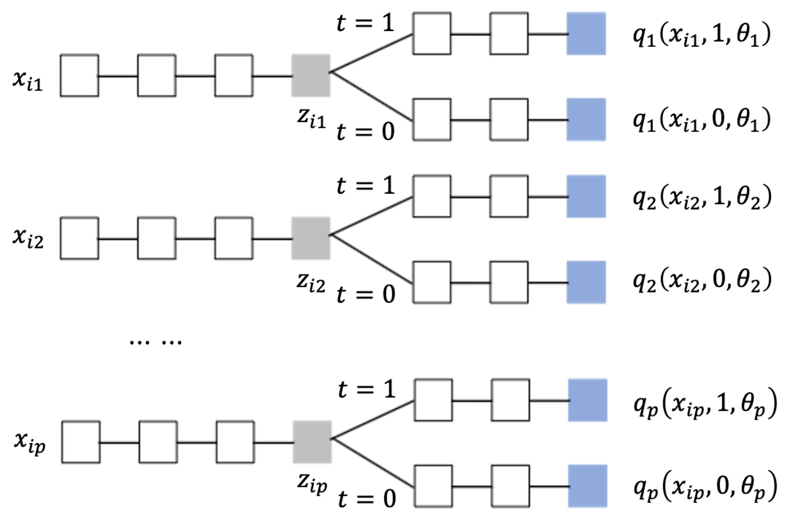
Figure 1: Architecture of additive neural network for predicting factual and counterfactual outcomes.

While deep learning models offer very impressive predictive performance, their power often comes at the expense of interpretability, or lack thereof. To balance the trade-off between predictive performance and interpretability, Agarwal et al., (2020) proposed the neural additive models (NAMs) combining the expressivity of DNNs with the interpretability of generalized additive models. Such models can be particularly useful for high stakes decision-making domains such as medicine where interpretability is highly desired or even necessary. As such, we propose to use NAMs to predict factual and counterfactual outcomes as follows,

$$\hat{Y}_{i}(a)=Q^{\text{NAM}}(\mathbf{X}_{i},a;\theta)=\sum_{j=1}^{p}q_{j}(x_{ij},a;\theta_{j})$$

where $X_{i}=(x_{i1},\cdots,x_{ip})\in\mathbb{R}^{p}$, $Q^{\text{NAM}}(\cdot,\cdot;\theta)$ is the fitted model, and $q_{j}$ is a univariate shape function. Figure 1 shows the architecture of our additive neural network models, where $z_{ij}\in\mathbb{R}$ is the shared representation for $q_{j}(\cdot,1;\theta_{j})$ and $q_{j}(\cdot,0;\theta_{j})$. We can replace the $Q^{\text{NN}}$ with $Q^{\text{NAM}}$ in the objective function (8) as appropriate.

3.3 Covariate Balancing Score Weighted Regularization

To further improve performance, we propose a refinement of the objective function in Section 3.2 through weighted regularization, which is motivated by the following weighted estimator of ATE,

$$\hat{\tau}_{\mathbf{w}}=\frac{1}{n_{1}}\sum_{i=1}^{n}w_{i}Y_{i}A_{i}-\frac{1}{n_{0}}\sum_{i=1}^{n}w_{i}Y_{i}(1-A_{i}).$$ (9)

We define the regularization term $\gamma(\mathbf{Y}_{i},A_{i},\mathbf{X}_{i};\theta,\epsilon)$ as follows,

$$\gamma(\mathbf{Y}_{i},A_{i},\mathbf{X}_{i};\theta,\epsilon)=(Y_{i}-\tilde{Q}(\mathbf{X}_{i},A_{i},\theta))^{2}.$$

Here, $\tilde{Q}(\mathbf{X}_{i},A_{i};\theta)=Q^{\text{NN}}(\mathbf{X}_{i},A_{i};\theta)+\epsilon\left(\frac{w_{i}A_{i}n}{n_{1}}-\frac{w_{i}(1-A_{i})n}{n_{0}}\right)$, where the second term can be viewed as a calibration term and $\epsilon$ is a tuning parameter.

Then the refined objective function is defined as follows,

$$\begin{split}\hat{\theta},\hat{\mathbf{w}},\hat{\epsilon}&=\operatorname*{arg\,min}_{\theta,\mathbf{w},\epsilon}\hat{R}(\mathbf{X},\mathbf{A};\theta,\mathbf{w})+\beta\frac{1}{n}\sum_{i=1}^{n}\gamma(\mathbf{Y}_{i},A_{i},\mathbf{X}_{i};\theta,\epsilon)\\ s.t.\quad&\sum_{i=1}^{n}w_{i}A_{i}=n_{1},\quad\sum_{i=1}^{n}w_{i}(1-A_{i})=n_{0},w_{i}\geq 0\\ \end{split}$$ (10)

where $\hat{R}(\mathbf{X},\mathbf{A};\theta,\mathbf{w})$ is defined in (8), and $\beta\in\mathbb{R}^{+}$ is a hyperparameter. It follows that our downstream estimator for ATE becomes

$$\hat{\tau}^{\text{wreg}}=\frac{1}{n}\sum_{i=1}^{n}\left(\tilde{Q}(\mathbf{X}_{i},1;\theta)-\tilde{Q}(\mathbf{X}_{i},0;\theta)\right).$$

The idea behind the weighted regularization process can be understood as follows. Recall the general procedure for estimating treatment effect has two steps: 1) fit models for the conditional outcome and balancing score; 2) plug the fitted models into a downstream estimator. Of note, there is a large body of literature on semi-parametric statistical methods for estimation of ATE (Kennedy,, 2016). In this work, we focus on the non-parametric estimator in (9) that uses energy distance balancing scores. Since this estimator does not require correct specification of the treatment assignment model, it is more robust than the Dragonnet model and target regularization in Shi et al., (2019).

Of particular note, under some mild conditions, the estimator $\hat{\tau}$ is expected to have some desirable asymptotic properties such as

• Robustness of the estimator, since the energy distance balancing score weight is non-parametric;

• Efficiency: $\hat{\tau}$ has the lowest variance of any consistent estimator of $\tau$. This means that $\hat{\tau}$ is the most data efficient estimator.

In particular, two important conditions are needed for these properties to hold: 1) $\hat{Q}$ and $\hat{\mathbf{w}}$ are consistent estimators of outcomes and balancing score; 2) the following non-parametric estimating equation is satisfied:

$$\begin{split}&\frac{1}{n}\sum_{i=1}^{n}\Bigg{(}\hat{Q}(\mathbf{X}_{i},1;\theta)-\hat{Q}(\mathbf{X}_{i},0;\theta)+\left(\frac{w_{i}A_{i}n}{n_{1}}-\frac{w_{i}(1-A_{i})n}{n_{0}}\right)(Y_{i}-\hat{Q}(\mathbf{X}_{i},A_{i};\theta))-\tau\Bigg{)}=0\end{split}$$ (11)

More details can be found in Van der Laan and Rose, (2011) and Chernozhukov et al., (2017). The most important observation here is that minimizing the modified objective (10) would force $\tilde{Q}$, $\hat{\mathbf{w}}$, and $\hat{\tau}^{\text{wreg}}$ to satisfy the estimating equation (11) because

$$\frac{\partial}{\partial\epsilon}\left(\hat{R}(\mathbf{X};\theta,\mathbf{w})+\beta\frac{1}{n}\sum_{i=1}^{n}\gamma(\mathbf{Y}_{i},A_{i},\mathbf{X}_{i};\theta,\epsilon)\right)=0.$$

As long as $\tilde{Q}$ and $\hat{\mathbf{w}}$ are consistent, by imposing the weighted regularization process, the estimator $\hat{\tau}^{\text{wreg}}$ is expected to have the aforementioned desirable asymptotic properties. More detailed discussions about the rationale for this regularization process can be found in Shi et al., (2019).

4 Numerical Experiments

We conduct numerical experiments to demonstrate the advantages of our proposed model compared to current state-of-the-art. Since ground truth causal effects are in general unavailable in real-world data, our experiments are conducted using semi-synthetic data derived from the Infant Health and Development Program (IHDP) and from the 2018 Atlantic Causal Inference Conference (ACIC) competition, two popular benchmark datasets for assessing causal inference methods.

IHDP. IHDP is a semi-synthetic dataset constructed from the Infant Health and Development Program, a randomized experiment started in 1985. Hill, (2011) introduced this data in their 2011 paper. In this program, the treated group was provided with intensive high-quality child care and home visits from trained specialists. At the end of the intervention, when the children were three years old, the intervention was deemed successful in raising cognitive test scores of treated children in comparison to controls. The dataset includes numerous measurements on participants such as birth weight, neonatal health index, first born weeks born preterm, head circumference, sex and twin status. It also contains information of mother’s behaviors engaged in during the pregnancy such as smoking status, alcohol usage and drug usage. The data generating process of the synthetic part of the data can be found in Hill, (2011). The data has 747 observations with 26 features.

ACIC 2018. This dataset was developed from the 2018 Atlantic Causal Inference Conference competition. The dataset include real-world clinical measurements taken from the Linked Birth and Infant Death Data (LBIDD) (Mathews and Atkinson,, 1998), e.g., infant mortality statistics from the linked birth/infant death data set (linked file) for the 1999 period, broken down by a variety of maternal and infant characteristics. In addition, it includes demographics of mothers and infants such as education, prenatal care, race, birth weight and days of born preterm. The outcome is the mortality rate. The treatment/exposure is the race of mothers (black or white). The synthetic part of the data is generated from 63 distinct data generating process settings. We follow the same selection criterion as in Shi et al., (2019), that is, we randomly pick 3 datasets of size either 5,000 and 10,000.

4.1 Interpretability

The interpreability of NAMs is due, in part, to the fact that it enables visualization of the impact of individual features on estimation of ATE. Since each feature is handled independently by a learned shape function parameterized by a neural net, plotting the individual shape functions offers a natural way to visualize their impact. These shape function plots can provide an exact description of how NAMs estimate the ATE, not merely just an explanation. This helps, for example, an decision-maker, say from medicine, to understand how to interpret the models and understand exactly how the estimated ATE is associated with risk factors.

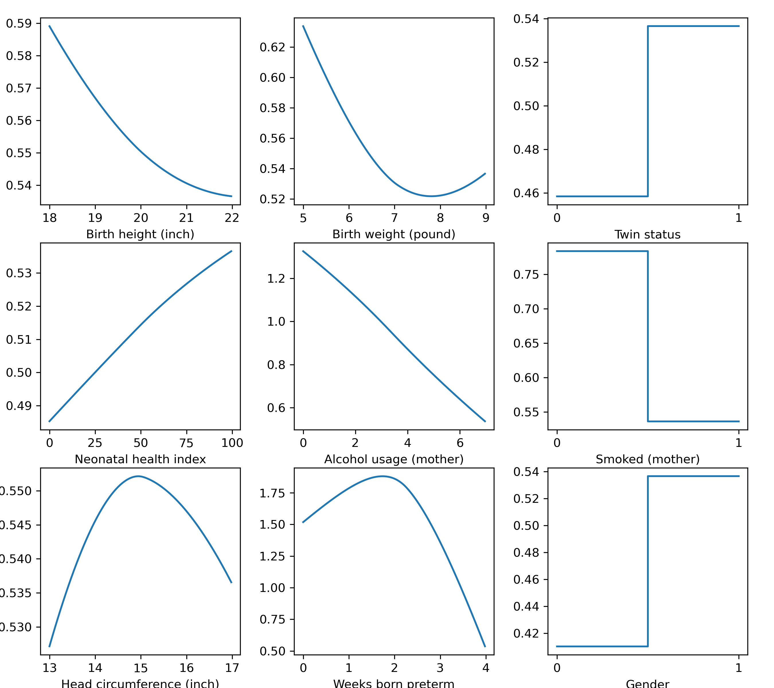
Figure 2: Impact of selected features on estimation of treatment effect on cognitive test scores in IHDP using NAM models. The $y-$axis represents the average treatment effect that attributed to each selected feature. (Gender: 0-male, 1-female)

We analyze the IHDP data using our proposed model. Figure 2 presents the aforementioned plots to demonstrate how to interpret the results from NAMs. First, by removing the mean score for each graph (i.e., each feature) across the entire training dataset, we set the average score for each plot in Figure 2 (i.e., each feature) to zero. A single bias term is then added to the model to make individual shape functions identifiable, so that the average prediction across all data points matches the observed baseline. This makes the interpretation of each term much easier.

In Figure 2, we plot each learned shape function $q_{j}(x_{ij},1;\theta_{j})-q_{j}(x_{ij},0;\theta_{j})$ against $x_{ij}$ for an ensemble of neural additive model using blue line. This enables us to determine when the ensemble models learned the same shape function and when they diverged. By plotting each shape function, we are able to interpret how model estimates treatment effect based on the contributions from each observed covariate such as birth weight, birth height and neonatal health index.

4.2 Treatment Effect Estimation

We further compare our proposed approach (with/without weighted regularization process) with several current state-of-the-art methods for estimating ATE: 1) BART, the Bayesian Additive Regression Tree (BART) by Chipman et al., (2010); 2) CBPS, covariate balancing propensity score (CBPS) by Imai and Ratkovic, (2014); 3) CF, the causal forest model by Sharma et al., (2019) motivated by generalized random forest from Athey et al., (2019); 4) SITE, a local similarity preserved ITE estimation by Yao et al., (2018); 5) GANITE, generative adversarial nets for the estimation of ITE by Yoon et al., (2018); 6) Perfect Matching, a method for training neural networks for counterfactual inference by Schwab et al., (2018); 7) DRAGONNET, the deep neural network structure model by Shi et al., (2019) with target regularization; 8) TARNET, the deep neural network model by Shalit et al., (2017); 9) FlexTENet, flexible approach for CATE estimation by Curth and van der Schaar, (2021).

Results Our experiment results in analyses of the IHDP and ACIC datasets are summarized in Table 1. For IHDP, we randomly split the data into training set, testing set and validating set with the equal proportion (i.e. $1/3$ for each). For ACIC, we use all the data as training set and estimate the ATE. We report the mean absolute error $|\hat{\tau}-\tau|$ in Table 1. Our results show that our proposed model with weighted regularization outperforms all the existing models included as it has the lowest bias of estimation for ATE in both the IHDP and ACIC 2018 datasets. Actually, even our base model (8) without weighted regularization yields nearly close to the best performance among all the other methods, suggesting the advantage of our new objective function in Section 3.2. In addition, our results also shows that the weighted regularization in the refined model (10) improves the performance of our base model (8), and the improvement is more pronounced for ACIC. Moreover, in comparison to fully-connected neural network models, NAMs are inherently interpretable while suffering a little loss in estimation accuracy when applied to both IHDP and ACIC, demonstrating the trade-off between interpreability and accuracy. Our model with regularization and NAMs outperforms all the other models with NAMs, which is particularly pronounced in ACIC.

Table 1: Performance on estimation of ATE in terms of the mean absolute error $|\hat{\tau}-\tau|$ across 200 datasets. For all deep neural network models, there are 3 hidden layers with 100 hidden units; the hyperparameter $\alpha,\beta$ are 0.05 and 1. The deep neural network models are trained using stochastic gradient descent with momentum. The causal forest is implemented using the package from Sharma et al., (2019); BART is implemented using the package from Sparapani et al., (2021). For comparisons, the deep neural network models used in the methods denoted by ^∗ are changed to NAMs.

Method	IHDP	ACIC
CLASSICAL ML MODELS
BART (Chipman et al.,, 2010)	$0.95\pm.04$	$1.32\pm.04$
CBPS (Imai and Ratkovic,, 2014)	$0.84\pm.03$	$1.25\pm.03$
CF (Sharma et al.,, 2019)	$0.79\pm.03$	$1.15\pm.03$
DEEP LEARNING MODELS
SITE (Yao et al.,, 2018)	$0.32\pm.02$	$0.51\pm.02$
GANITE (Yoon et al.,, 2018)	$0.51\pm.03$	$0.81\pm.03$
Perfect Match (Schwab et al.,, 2018)	$0.40\pm.02$	$0.71\pm.02$
DRAGONNET (Shi et al.,, 2019)	$0.20\pm.01$	$0.35\pm.01$
DRAGONNET∗ (Shi et al.,, 2019)	$0.31\pm.01$	$0.56\pm.01$
TARNET∗ (Shalit et al.,, 2017)	$0.46\pm.02$	$0.77\pm.02$
FlexTENet∗ (Curth and van der Schaar,, 2021)	$0.49\pm.03$	$0.79\pm.03$
Our model∗ (without regularization)	$\mathbf{0.39\pm.02}$	$\mathbf{0.53\pm.02}$
Our model∗ (with regularization)	$\mathbf{0.29\pm.02}$	$\mathbf{0.46\pm.02}$
Our model (without regularization)	$\mathbf{0.27\pm.02}$	$\mathbf{0.44\pm.02}$
Our model (with regularization)	$\mathbf{0.18\pm.02}$	$\mathbf{0.32\pm.02}$

5 Discussion and Conclusion

In this paper, we propose a new covariate-balancing-aware interpretable deep learning approach for estimating ATE. By leveraging appealing properties of the weighted energy distance, we derive a generalization error bound for the bias of estimation of ATE that is sharper than the existing work. Our theoretical analysis motivated the development of our new models including a new objective function and a energy distance propensity score weighted regularization. In addition,to balance trade-off between the predictive performance and interpreability, neural additive models can be used for predicting potential outcomes in our approach. Our numerical results including ablation experiments demonstrate the advantages of the proposed loss function and the weighted regularization.

There are some promising future extensions of our work. For example, a possible extension is to incorporate instrumental variables for the explanation for hidden confounders. Recall our work is under “strong ignorability” assumption. Hartford et al., (2017) equipped their model with instrumental variables for counterfactual prediction under additive hidden bias model assumption. However, such assumption is somehow not applicable in most real cases in comparison to traditional instrumental variables assumptions such as mean independence assumption or monotonicity assumption. Conducting theoretical analysis for the bias of interval estimation of ATE under instrumental variable framework will be our next goal.

6 Supplementary Materials for “Covariate-Balancing-Aware Interpretable Deep Learning Models for Treatment Effect Estimation"

6.1 Covariate Balancing Propensity Score with Deep Neural Network

Covariate balancing propensity score (CBPS) can be viewed as an adjustment for propensity score model based on the distributions of treated and control units. To equip deep neural network models with covariate balancing propensity score, let $Q^{\text{NN}}(\mathbf{X}_{i},A_{i};\theta)$ denote the predicted outcomes using neural network, and $g(\mathbf{X}_{i};\theta)$ be the estimated propensity score, then we train our neural network by minimizing the objective function

$$\hat{\theta}=\operatorname*{arg\,min}_{\theta}\hat{R}(\mathbf{X},\mathbf{A};\theta),\quad\text{where}$$

$$\hat{R}(\mathbf{X},\mathbf{A};\theta) =\frac{1}{n}\sum_{i=1}^{n}(Q^{\text{NN}}(\mathbf{X}_{i},A_{i};\theta)-Y_{i})^{2}+\bar{h}_{\theta}(\mathbf{A},\mathbf{X})^{\top}\Sigma_{\theta}(\mathbf{A},\mathbf{X})^{-1}\bar{h}_{\theta}(\mathbf{A},\mathbf{X})$$

$$\bar{h}_{\theta}(\mathbf{A},\mathbf{X}) =\frac{1}{n}\sum_{i=1}^{n}h_{\theta}(A_{i},\mathbf{X}_{i})$$

$$h_{\theta}(A_{i},\mathbf{X}_{i}) =\binom{\frac{\partial g}{\partial\theta}(\mathbf{X}_{i};\theta)}{\frac{A_{i}-g(\mathbf{X}_{i};\theta)}{g(\mathbf{X}_{i};\theta)(1-g(\mathbf{X}_{i};\theta))}\mathbf{X}_{i}}$$

$$\Sigma_{\theta}(\mathbf{A},\mathbf{X}) =\frac{1}{n}\sum_{i=1}^{N}\mathbb{E}\left(g(\mathbf{X}_{i};\theta)g(\mathbf{X}_{i};\theta)^{\top}|\mathbf{X}_{i}\right).$$

It is motivated by the Method of Moments. We match the first moment of the distributions of treated units and control units. Details of CBPS can be found in Imai and Ratkovic, (2014).

6.2 Proof of Lemma 1

Proof.

According to the concept of expected factual and counterfactual losses in Definition 1, the concepts of expected factual (counterfactual) treated and control losses are immediately followed:

$$R_{F}(\hat{\mu}_{1})=\int_{\mathbb{R}^{p}}l_{\hat{\mu}_{1}}(\mathbf{x})\,dF_{1}(\mathbf{x})$$

$$R_{F}(\hat{\mu}_{0})=\int_{\mathbb{R}^{p}}l_{\hat{\mu}_{0}}(\mathbf{x})\,dF_{0}(\mathbf{x})$$

$$R_{CF}(\hat{\mu}_{1})=\int_{\mathbb{R}^{p}}l_{\hat{\mu}_{1}}(\mathbf{x})\,dF_{0}(\mathbf{x})$$

$$R_{CF}(\hat{\mu}_{0})=\int_{\mathbb{R}^{p}}l_{\hat{\mu}_{0}}(\mathbf{x})\,dF_{1}(\mathbf{x})$$

The connections between expected factual (counterfactual) treated losses and expected factual (counterfactual) control losses are:

$$R_{F}(\hat{\mu}_{a})=P_{0}\,R_{F}(\hat{\mu}_{0})+P_{1}\,R_{F}(\hat{\mu}_{1})$$

$$R_{CF}(\hat{\mu}_{a})=P_{1}\,R_{CF}(\hat{\mu}_{0})+P_{0}\,R_{CF}(\hat{\mu}_{1})$$

where $P_{1}\equiv\mathbb{P}(A=1),P_{0}\equiv\mathbb{P}(A=0)$.

Then if we do subtraction between $R_{CF}(\hat{\mu}_{a})$ and $R_{F}(\hat{\mu}_{a})$, then

$$R_{CF}(\hat{\mu}_{a})-R_{F}(\hat{\mu}_{a})=\left[P_{0}\,R_{CF}(\hat{\mu}_{1})+P_{1}\,R_{CF}(\hat{\mu}_{0})\right]-\left[P_{0}\,R_{F}(\hat{\mu}_{1})+P_{1}\,R_{F}(\hat{\mu}_{0})\right]$$

$$= P_{0}\left[R_{CF}(\hat{\mu}_{1})-R_{F}(\hat{\mu}_{1})\right]+P_{1}\left[R_{CF}(\hat{\mu}_{0})-P_{1}R_{F}(\hat{\mu}_{0})\right]$$

$$= P_{0}\left[\int_{\mathbb{R}^{p}}l_{\hat{\mu}_{1}}(\mathbf{x})\,dF_{0}(\mathbf{x})-\int_{\mathbb{R}^{p}}l_{\hat{\mu}_{1}}(\mathbf{x})\,dF_{1}(\mathbf{x})\right]+P_{1}\left[\int_{\mathbb{R}^{p}}l_{\hat{\mu}_{0}}(\mathbf{x})\,dF_{1}(\mathbf{x})-\int_{\mathbb{R}^{p}}l_{\hat{\mu}_{0}}(\mathbf{x})\,dF_{0}(\mathbf{x})\right]$$

$$= -P_{0}\int_{\mathbb{R}^{p}}l_{\hat{\mu}_{1}}(\mathbf{x})\,d[F_{1}-F_{0}](\mathbf{x})+P_{1}\int_{\mathbb{R}^{p}}l_{\hat{\mu}_{0}}(\mathbf{x})\,d[F_{1}-F_{0}](\mathbf{x})$$

$$= \int_{\mathbb{R}^{p}}[-P_{0}l_{\hat{\mu}_{1}}+P_{1}l_{\hat{\mu}_{0}}](\mathbf{x})\,d[F_{1}-F_{0}](\mathbf{x})$$

$$= \int_{\mathbb{R}^{p}}[-P_{0}l_{\hat{\mu}_{1}}+P_{1}l_{\hat{\mu}_{0}}](\mathbf{x})\,d[F-F_{0}](\mathbf{x})-\int_{\mathbb{R}^{p}}[-P_{0}l_{\hat{\mu}_{1}}+P_{1}l_{\hat{\mu}_{0}}](\mathbf{x})\,d[F-F_{1}](\mathbf{x}).$$

Let $g(\mathbf{x})=[-P_{0}l_{\hat{\mu}_{1}}+P_{1}l_{\hat{\mu}_{0}}](\mathbf{x})$, accoring to Theorem 4 (Koksma-Hlawka) by Mak and Joseph, (2018):

$$\left|\int_{\mathbb{R}^{p}}[-P_{0}l_{\hat{\mu}_{1}}+P_{1}l_{\hat{\mu}_{0}}](\mathbf{x})\,d[F-F_{0}](\mathbf{x})\right|=\left|\int_{\mathbb{R}^{p}}g(\mathbf{x})\,d[F-F_{0}](\mathbf{x})\right|$$

$$\leq \|\partial^{p}g/\partial\mathbf{x}^{p}\|_{2}\left(\int_{\mathbb{R}^{p}}(F(\mathbf{x})-F_{0}(\mathbf{x}))^{2}d\mathbf{x}\right)^{1/2}=\frac{\|\partial^{p}g/\partial\mathbf{x}^{p}\|_{2}}{\sqrt{2}}\sqrt{\mathcal{E}(F,F_{0})}=C_{l_{\hat{\mu}_{a}}}\sqrt{\mathcal{E}(F,F_{0})}$$

Similarly,

$$\left|\int_{\mathbb{R}^{p}}[-P_{0}l_{\hat{\mu}_{1}}+P_{1}l_{\hat{\mu}_{0}}](\mathbf{x})\,d[F-F_{1}](\mathbf{x})\right|\leq\frac{\|\partial^{p}g/\partial\mathbf{x}^{p}\|_{2}}{\sqrt{2}}\sqrt{\mathcal{E}(F,F_{1})}=C_{l_{\hat{\mu}_{a}}}\sqrt{\mathcal{E}(F,F_{1})}$$

where $C_{l_{\hat{\mu}_{a}}}=\|\partial^{p}[-P_{0}l_{\hat{\mu}_{1}}+P_{1}l_{\hat{\mu}_{0}}](\mathbf{x})/\partial\mathbf{x}^{p})\|_{2}/\sqrt{2}$ is a constant. According to the triangle inequality,

$$R_{CF}(\hat{\mu}_{a})-\left[P_{0}\,R_{F}(\hat{\mu}_{1})+P_{1}\,R_{F}(\hat{\mu}_{0})\right]\leq\left|R_{CF}(\hat{\mu}_{a})-\left[P_{0}\,R_{F}(\hat{\mu}_{1})+P_{1}\,R_{F}(\hat{\mu}_{0})\right]\right|$$

$$= \Big{|}\int_{\mathbb{R}^{p}}[-P_{0}l_{\hat{\mu}_{1}}+P_{1}l_{\hat{\mu}_{0}}](\mathbf{x})\,d[F-F_{0}](\mathbf{x})-\int_{\mathbb{R}^{p}}[-P_{0}l_{\hat{\mu}_{1}}+P_{1}l_{\hat{\mu}_{0}}](\mathbf{x})\,d[F-F_{1}](\mathbf{x})\Big{|}$$

$$\leq \left|\int_{\mathbb{R}^{p}}[-P_{0}l_{\hat{\mu}_{1}}+P_{1}l_{\hat{\mu}_{0}}](\mathbf{x})\,d[F-F_{0}](\mathbf{x})\right|+\left|\int_{\mathbb{R}^{p}}[-P_{0}l_{\hat{\mu}_{1}}+P_{1}l_{\hat{\mu}_{0}}](\mathbf{x})\,d[F-F_{1}](\mathbf{x})\right|$$

$$\leq C_{l_{\hat{\mu}_{a}}}\left(\sqrt{\mathcal{E}(F,F_{0})}+\sqrt{\mathcal{E}(F,F_{1})}\right)$$

To prove the result when $n\to\infty$ with weights, similarly, the weighted expected factual (counterfactual) treated and control losses and their relations are given as:

$$R_{F}(\hat{\mu}_{1},\mathbf{w})=\int_{\mathbb{R}^{p}}l_{\hat{\mu}_{1}}(\mathbf{x})\,dF_{n,1,\mathbf{w}}(\mathbf{x})$$

$$R_{F}(\hat{\mu}_{0},\mathbf{w})=\int_{\mathbb{R}^{p}}l_{\hat{\mu}_{0}}(\mathbf{x})\,dF_{n,0,\mathbf{w}}(\mathbf{x})$$

$$R_{CF}(\hat{\mu}_{1},\mathbf{w})=\int_{\mathbb{R}^{p}}l_{\hat{\mu}_{1}}(\mathbf{x})dF_{n,0,\mathbf{w}}(\mathbf{x})$$

$$R_{CF}(\hat{\mu}_{0},\mathbf{w})=\int_{\mathbb{R}^{p}}l_{\hat{\mu}_{0}}(\mathbf{x})dF_{n,1,\mathbf{w}}(\mathbf{x})$$

$$R_{F}(\hat{\mu}_{a},\mathbf{w})=P_{0}\,R_{F}(\hat{\mu}_{0},\mathbf{w})+P_{1}\,R_{F}(\hat{\mu}_{1},\mathbf{w})$$

$$R_{CF}(\hat{\mu}_{a},\mathbf{w})=P_{1}\,R_{CF}(\hat{\mu}_{0},\mathbf{w})+P_{0}\,R_{CF}(\hat{\mu}_{1},\mathbf{w}).$$

Then again, we can do subtraction between $R_{CF}(\hat{\mu}_{a},\mathbf{w})$ and $R_{F}(\hat{\mu}_{a},\mathbf{w})$:

$$R_{CF}(\hat{\mu}_{a},\mathbf{w})-R_{F}(\hat{\mu}_{a},\mathbf{w})$$

$$= \int_{\mathbb{R}^{p}}[-P_{0}l_{\hat{\mu}_{1}}+P_{1}l_{\hat{\mu}_{0}}](\mathbf{x})\,d[F_{n}-F_{n,0,\mathbf{w}}](\mathbf{x})-\int_{\mathbb{R}^{p}}[-P_{0}l_{\hat{\mu}_{1}}+P_{1}l_{\hat{\mu}_{0}}](\mathbf{x})\,d[F_{n}-F_{n,1,\mathbf{w}}](\mathbf{x}).$$

Then by Lemma 3.3 in Huling and Mak, (2020),

$$\left|\int_{\mathbb{R}^{p}}[-P_{0}l_{\hat{\mu}_{1}}+P_{1}l_{\hat{\mu}_{0}}](\mathbf{x})\,d[F_{n}-F_{n,0,\mathbf{w}}](\mathbf{x})\right|=C_{l_{\hat{\mu}_{a}}}\sqrt{\mathcal{E}(F_{n},F_{n,0,\mathbf{w}})}$$

and

$$\left|\int_{\mathbb{R}^{p}}[-P_{0}l_{\hat{\mu}_{1}}+P_{1}l_{\hat{\mu}_{0}}](\mathbf{x})\,d[F_{n}-F_{n,1,\mathbf{w}}](\mathbf{x})\right|=C_{l_{\hat{\mu}_{a}}}\sqrt{\mathcal{E}(F_{n},F_{n,1,\mathbf{w}})}$$

Finally,

$$R_{CF}(\hat{\mu}_{a},\mathbf{w})-R_{F}(\hat{\mu}_{a},\mathbf{w})\leq\left|R_{CF}(\hat{\mu}_{a},\mathbf{w})-R_{CF}(\hat{\mu}_{a},\mathbf{w})-R_{F}(\hat{\mu}_{a},\mathbf{w})\right|$$

$$= \Big{|}\int_{\mathbb{R}^{p}}[-P_{0}l_{\hat{\mu}_{1}}+P_{1}l_{\hat{\mu}_{0}}](\mathbf{x})\,d[F_{n}-F_{n,0,\mathbf{w}}](\mathbf{x})-\int_{\mathbb{R}^{p}}[-P_{0}l_{\hat{\mu}_{1}}+P_{1}l_{\hat{\mu}_{0}}](\mathbf{x})\,d[F_{n}-F_{n,1,\mathbf{w}}](\mathbf{x})\Big{|}$$

$$\leq \left|\int_{\mathbb{R}^{p}}[-P_{0}l_{\hat{\mu}_{1}}+P_{1}l_{\hat{\mu}_{0}}](\mathbf{x})\,d[F_{n}-F_{n,0,\mathbf{w}}](\mathbf{x})\right|-\left|\int_{\mathbb{R}^{p}}[-P_{0}l_{\hat{\mu}_{1}}+P_{1}l_{\hat{\mu}_{0}}](\mathbf{x})\,d[F_{n}-F_{n,1,\mathbf{w}}](\mathbf{x})\right|$$

$$\leq C_{l_{\hat{\mu}_{a}}}\left(\sqrt{\mathcal{E}(F_{n},F_{n,0,\mathbf{w}})}+\sqrt{\mathcal{E}(F_{n},F_{n,1,\mathbf{w}})}\right)$$

∎

6.3 Proof of Theorem 1

Before proving Theorem 1, it will be helpful to state the following definition and claims.

Definition 6.

The expected variance of $Y(a)$ with respect to the distribution $p(\mathbf{x},a)$ is

$$\sigma_{Y(a)}^{2}(p(\mathbf{x},a))=\int_{\mathbb{R}^{p}\times\mathcal{Y}}(Y(a)-\mu_{a}(\mathbf{x}))^{2}p(Y(a)|\mathbf{x})dY(a)dF_{a}(\mathbf{x})$$

and we further define

$$\sigma_{Y(a)}^{2}=\min\{\sigma_{Y(a)}^{2}(p(\mathbf{x},a)),\sigma_{Y(a)}^{2}(p(\mathbf{x},1-a))\}$$

$$\sigma_{Y}^{2}=\min\{\sigma_{Y(1)}^{2},\sigma_{Y(0)}^{2}\}.$$

Claim 1.

Given all conditions of Lemma 1, the following two equalities hold:

$$\int_{\mathbb{R}^{p}\times\{0,1\}}\lVert\hat{\mu}_{a}(\mathbf{x})-\mu_{a}(\mathbf{x})\rVert_{2}^{2}\,dF_{a}(\mathbf{x})\,da=R_{F}(\hat{\mu}_{a})-\sigma_{Y(a)}^{2}(p(\mathbf{x},a))$$

and

$$\int_{\mathbb{R}^{p}\times\{0,1\}}\lVert\hat{\mu}_{a}(\mathbf{x})-\mu_{a}(\mathbf{x})\rVert_{2}^{2}\,dF_{1-a}(\mathbf{x})\,da=R_{CF}(\hat{\mu}_{a})-\sigma_{Y(a)}^{2}(p(\mathbf{x},1-a))$$

Proof of Claim 1.

$$R_{F}(\hat{\mu}_{a})= \int_{\mathbb{R}^{p}\times\{0,1\}\times\mathcal{Y}}\lVert\hat{\mu}_{a}(\mathbf{x})-Y(a)\rVert_{2}^{2}\,p(Y(a)|\mathbf{x})\,dF_{1-a}(\mathbf{x})\,dY(a)\,da$$

$$= \int_{\mathbb{R}^{p}\times\{0,1\}\times\mathcal{Y}}\lVert\hat{\mu}_{a}(\mathbf{x})-\mu_{a}(\mathbf{x})\rVert_{2}^{2}\,p(Y(a)|\mathbf{x})\,dF_{1-a}(\mathbf{x})\,dY(a)\,da$$

$$+\int_{\mathbb{R}^{p}\times\{0,1\}\times\mathcal{Y}}\lVert\mu_{a}(\mathbf{x})-Y(a)\rVert_{2}^{2}\,p(Y(a)|\mathbf{x})\,dF_{1-a}(\mathbf{x})\,dY(a)\,da$$

$$= \int_{\mathbb{R}^{p}\times\{0,1\}}\lVert\hat{\mu}_{a}(\mathbf{x})-\mu_{a}(\mathbf{x})\rVert_{2}^{2}\,dF_{1-a}(\mathbf{x})\,da+\sigma_{Y(1)}^{2}(p(\mathbf{x},a))+\sigma_{Y(0)}^{2}(p(\mathbf{x},a))$$

$$= \int_{\mathbb{R}^{p}\times\{0,1\}}\lVert\hat{\mu}_{a}(\mathbf{x})-\mu_{a}(\mathbf{x})\rVert_{2}^{2}\,p(Y(a)|\mathbf{x})\,dF_{1-a}(\mathbf{x})\,da+\sigma_{Y(a)}^{2}(p(\mathbf{x},a))$$

Therefore,

$$\int_{\mathbb{R}^{p}\times\{0,1\}}\lVert\hat{\mu}_{a}(\mathbf{x})-\mu_{a}(\mathbf{x})\rVert_{2}^{2}\,dF_{a}(\mathbf{x})\,da=R_{F}(\hat{\mu}_{a})-\sigma_{Y(a)}^{2}(p(\mathbf{x},a))$$

Similarly,

$$\int_{\mathbb{R}^{p}\times\{0,1\}}\lVert\hat{\mu}_{a}(\mathbf{x})-\mu_{a}(\mathbf{x})\rVert_{2}^{2}\,dF_{1-a}(\mathbf{x})\,da=R_{CF}(\hat{\mu}_{a})-\sigma_{Y(a)}^{2}(p(\mathbf{x},1-a))$$

∎

Claim 2.

Given all conditions of Lemma 1, the following inequality also holds:

$$R_{ATE}(\hat{\mu}_{a})\leq 2\left(R_{F}(\hat{\mu}_{a})+R_{CF}(\hat{\mu}_{a})-2\sigma_{Y}^{2}\right)$$

Proof of Claim 2.

$$R_{ATE}(\hat{\mu}_{a})= \int_{\mathbb{R}^{p}}\lVert\hat{\tau}(\mathbf{x})-\tau(\mathbf{x})\rVert_{2}^{2}\,dF(\mathbf{x})=\int_{\mathbb{R}^{p}}\lVert\left(\hat{\mu}_{1}(\mathbf{x})-\hat{\mu}_{0}(\mathbf{x})\right)-\left(\mu_{1}(\mathbf{x})-\mu_{0}(\mathbf{x})\right)\rVert_{2}^{2}\,dF(\mathbf{x})$$

$$= \int_{\mathbb{R}^{p}}\lVert\left(\hat{\mu}_{1}(\mathbf{x})-\mu_{1}(\mathbf{x})\right)-\left(\hat{\mu}_{0}(\mathbf{x})-\mu_{0}(\mathbf{x})\right)\rVert_{2}^{2}\,dF(\mathbf{x})$$

$$\leq 2\int_{\mathbb{R}^{p}}\lVert\hat{\mu}_{1}(\mathbf{x})-\mu_{1}(\mathbf{x})\rVert_{2}^{2}\,dF(\mathbf{x})+2\int_{\mathbb{R}^{p}}\lVert\hat{\mu}_{0}(\mathbf{x})-\mu_{0}(\mathbf{x})\rVert_{2}^{2}\,dF(\mathbf{x})$$

$$= 2\int_{\mathbb{R}^{p}}\lVert\hat{\mu}_{1}(\mathbf{x})-\mu_{1}(\mathbf{x})\rVert_{2}^{2}\,dF_{1}(\mathbf{x})+2\int_{\mathbb{R}^{p}}\lVert\hat{\mu}_{1}(\mathbf{x})-\mu_{1}(\mathbf{x})\rVert_{2}^{2}\,dF_{0}(\mathbf{x})$$

$$+2\int_{\mathbb{R}^{p}}\lVert\hat{\mu}_{0}(\mathbf{x})-\mu_{0}(\mathbf{x})\rVert_{2}^{2}\,dF_{1}(\mathbf{x})+2\int_{\mathbb{R}^{p}}\lVert\hat{\mu}_{0}(\mathbf{x})-\mu_{0}(\mathbf{x})\rVert_{2}^{2}\,dF_{0}(\mathbf{x})$$

$$= 2\int_{\mathbb{R}^{p}\times\{0,1\}}\lVert\hat{\mu}_{a}(\mathbf{x})-\mu_{a}(\mathbf{x})\rVert_{2}^{2}\,dF_{a}(\mathbf{x})\,da+2\int_{\mathbb{R}^{p}\times\{0,1\}}\lVert\hat{\mu}_{a}(\mathbf{x})-\mu_{a}(\mathbf{x})\rVert_{2}^{2}\,dF_{1-a}(\mathbf{x})\,da$$

$$\leq 2\left(R_{F}(\hat{\mu}_{a})-\sigma_{Y}^{2}\right)+2\left(R_{CF}(\hat{\mu}_{a})-\sigma_{Y}^{2}\right)$$

The last line is proved by Claim 1. ∎

Proof of Theorem 1.

According to Lemma 1 and its proof, we have

$$R_{CF}(\hat{\mu}_{a})\leq P_{0}\,R_{F}(\hat{\mu}_{1})+P_{1}\,R_{F}(\hat{\mu}_{0})+C_{l_{\hat{\mu}_{a}}}\left(\sqrt{\mathcal{E}(F,F_{0})}+\sqrt{\mathcal{E}(F,F_{1})}\right)$$

and

$$R_{F}(\hat{\mu}_{a})=P_{0}\,R_{F}(\hat{\mu}_{0})+P_{1}\,R_{F}(\hat{\mu}_{1})$$

then

$$R_{F}(\hat{\mu}_{a})+R_{CF}(\hat{\mu}_{a})\leq P_{0}\,R_{F}(\hat{\mu}_{1})+P_{1}\,R_{F}(\hat{\mu}_{0})+C_{l_{\hat{\mu}_{a}}}\left(\sqrt{\mathcal{E}(F,F_{0})}+\sqrt{\mathcal{E}(F,F_{1})}\right)$$

$$+P_{0}\,R_{F}(\hat{\mu}_{0})+P_{1}\,R_{F}(\hat{\mu}_{1})$$

$$= R_{F}(\hat{\mu}_{1})+R_{F}(\hat{\mu}_{0})+C_{l_{\hat{\mu}_{a}}}\left(\sqrt{\mathcal{E}(F,F_{0})}+\sqrt{\mathcal{E}(F,F_{1})}\right)$$

Therefore,

$$R_{ATE}(\hat{\mu}_{a})\leq 2\left(R_{CF}(\hat{\mu}_{a})-\sigma_{Y}^{2}\right)+2\left(R_{CF}(\hat{\mu}_{a})-\sigma_{Y}^{2}\right)$$

$$= 2\big{(}R_{F}(\hat{\mu}_{1})+R_{F}(\hat{\mu}_{0})+C_{l_{\hat{\mu}_{a}}}(\sqrt{\mathcal{E}(F,F_{0})}+\sqrt{\mathcal{E}(F,F_{1})})-2\sigma_{Y}^{2}\big{)}$$

$$= 2\left(R_{F}(\hat{\mu}_{1})+R_{F}(\hat{\mu}_{0})+C_{l_{\hat{\mu}_{a}}}\Big{(}\sqrt{\mathcal{E}(F,F_{0})}+\sqrt{\mathcal{E}(F,F_{1})}\Big{)}\right)$$

To prove the expected loss in estimation of average treatment effect with weight, Claim 3 will be given. The proof of Claim 3 is similar to Claim 1 and Claim 2.

Claim 3.

Under conditions of Lemma 1, the following equalities hold

$$\int_{\mathbb{R}^{p}\times\{0,1\}}\lVert\hat{\mu}_{a}(\mathbf{x})-\mu_{a}(\mathbf{x})\rVert_{2}^{2}\,dF_{n,a,\mathbf{w}}(\mathbf{x})\,da= R_{F}(\hat{\mu}_{a},\mathbf{w})-\sigma_{Y(a)}^{2}(p(\mathbf{x},a))$$

$$\int_{\mathbb{R}^{p}\times\{0,1\}}\lVert\hat{\mu}_{a}(\mathbf{x})-\mu_{a}(\mathbf{x})\rVert_{2}^{2}\,dF_{n,1-a,\mathbf{w}}(\mathbf{x})\,da= R_{CF}(\hat{\mu}_{a},\mathbf{w})-\sigma_{Y(a)}^{2}(p(\mathbf{x},1-a)),$$

and

$$R_{ATE}(\hat{\mu}_{a})= R_{ATE,n}(\hat{\mu}_{a})\leq 2\left(R_{F}(\hat{\mu}_{1},\mathbf{w})+R_{F}(\hat{\mu}_{0},\mathbf{w})-2\sigma_{Y}^{2}\right)$$

According to the result in Lemma 1 with weight, Claim 1, Claim 2 and Claim 3,

$$R_{F}(\hat{\mu}_{1},\mathbf{w})+R_{CF}(\hat{\mu}_{0},\mathbf{w})$$

$$\leq R_{F}(\hat{\mu}_{1},\mathbf{w})+R_{F}(\hat{\mu}_{0},\mathbf{w})+C_{l_{\hat{\mu}_{a}}}\sqrt{\mathcal{E}(F_{n},F_{n,0,\mathbf{w}})}+C_{l_{\hat{\mu}_{a}}}\sqrt{\mathcal{E}(F_{n},F_{n,1,\mathbf{w}})}$$

Therefore,

$$R_{ATE}(\hat{\mu}_{a})\leq 2\left(R_{F}(\hat{\mu}_{1},\mathbf{w})+R_{F}(\hat{\mu}_{0},\mathbf{w})-2\sigma_{Y}^{2}\right)$$

$$\leq 2\left(R_{F}(\hat{\mu}_{1},\mathbf{w})+R_{F}(\hat{\mu}_{0},\mathbf{w})+C_{l_{\hat{\mu}_{a}}}\Big{(}\sqrt{\mathcal{E}(F_{n},F_{n,0,\mathbf{w}})}+\sqrt{\mathcal{E}(F_{n},F_{n,1,\mathbf{w}})}\Big{)}\right)$$

∎

6.4 Experiment Details

The experiments are run using R (version of 4.1.0) and Python (Version of 3.8.5) on Intel(R) 8 Cores(TM) i7-9700F CPU (3.00GHz). We use R package ‘bartCause’ license GPL (>= 2) for BART, ‘CBPS’ license GPL (>= 2) for CBPS, and ‘grf’ license GPL-3 for Causal Forest. We also use Python codes for GANITE from https://github.com/jsyoon0823/GANITE, SITE from https://github.com/Osier-Yi/SITE, FlexTENet from https://github.com/AliciaCurth/CATENets, Perfect Match from https://github.com/d909b/perfect_match, and DRAGONNET from https://github.com/claudiashi57/dragonnet. IHDP data is available from https://github.com/claudiashi57/dragonnet/tree/master/dat/ihdp/csv, and ACIC 2018 data is avaialble from https://www.synapse.org/#!Synapse:syn11294478/wiki/486304.

References

• Agarwal et al., (2020) Agarwal, R., Frosst, N., Zhang, X., Caruana, R., and Hinton, G. E. (2020). Neural additive models: Interpretable machine learning with neural nets. arXiv preprint arXiv:2004.13912.
• Alaa and van der Schaar, (2017) Alaa, A. M. and van der Schaar, M. (2017). Bayesian inference of individualized treatment effects using multi-task gaussian processes. arXiv preprint arXiv:1704.02801.
• Alaa et al., (2017) Alaa, A. M., Weisz, M., and Van Der Schaar, M. (2017). Deep counterfactual networks with propensity-dropout. arXiv preprint arXiv:1706.05966.
• Athey et al., (2019) Athey, S., Tibshirani, J., and Wager, S. (2019). Generalized random forests. The Annals of Statistics, 47(2):1148–1178.
• Bica et al., (2020) Bica, I., Jordon, J., and van der Schaar, M. (2020). Estimating the effects of continuous-valued interventions using generative adversarial networks. arXiv preprint arXiv:2002.12326.
• Bu et al., (2021) Bu, Z., Xu, S., and Chen, K. (2021). A dynamical view on optimization algorithms of overparameterized neural networks. In International Conference on Artificial Intelligence and Statistics, pages 3187–3195. PMLR.
• Chernozhukov et al., (2017) Chernozhukov, V., Chetverikov, D., Demirer, M., Duflo, E., Hansen, C., and Newey, W. (2017). Double/debiased/neyman machine learning of treatment effects. American Economic Review, 107(5):261–65.
• Chipman et al., (2010) Chipman, H. A., George, E. I., and McCulloch, R. E. (2010). Bart: Bayesian additive regression trees. The Annals of Applied Statistics, 4(1):266–298.
• Cox, (1958) Cox, D. R. (1958). Planning of experiments. Wiley.
• Cramér, (1928) Cramér, H. (1928). On the composition of elementary errors: Statistical applications. Almqvist and Wiksell.
• Curth and van der Schaar, (2021) Curth, A. and van der Schaar, M. (2021). On inductive biases for heterogeneous treatment effect estimation. Advances in Neural Information Processing Systems, 34.
• Du et al., (2018) Du, S. S., Zhai, X., Poczos, B., and Singh, A. (2018). Gradient descent provably optimizes over-parameterized neural networks. arXiv preprint arXiv:1810.02054.
• Farrell et al., (2018) Farrell, M. H., Liang, T., and Misra, S. (2018). Deep neural networks for estimation and inference: Application to causal effects and other semiparametric estimands. arXiv preprint arXiv:1809.09953.
• Hartford et al., (2017) Hartford, J., Lewis, G., Leyton-Brown, K., and Taddy, M. (2017). Deep iv: A flexible approach for counterfactual prediction. In International Conference on Machine Learning, pages 1414–1423. PMLR.
• Hill, (2011) Hill, J. L. (2011). Bayesian nonparametric modeling for causal inference. Journal of Computational and Graphical Statistics, 20(1):217–240.
• Huling and Mak, (2020) Huling, J. D. and Mak, S. (2020). Energy balancing of covariate distributions. arXiv preprint arXiv:2004.13962.
• Imai and Ratkovic, (2014) Imai, K. and Ratkovic, M. (2014). Covariate balancing propensity score. Journal of the Royal Statistical Society: Series B (Statistical Methodology), 76(1):243–263.
• Johansson et al., (2016) Johansson, F., Shalit, U., and Sontag, D. (2016). Learning representations for counterfactual inference. In International conference on machine learning, pages 3020–3029. PMLR.
• Johansson et al., (2020) Johansson, F. D., Shalit, U., Kallus, N., and Sontag, D. (2020). Generalization bounds and representation learning for estimation of potential outcomes and causal effects. arXiv preprint arXiv:2001.07426.
• Kaddour et al., (2021) Kaddour, J., Zhu, Y., Liu, Q., Kusner, M. J., and Silva, R. (2021). Causal effect inference for structured treatments. Advances in Neural Information Processing Systems, 34.
• Kennedy, (2016) Kennedy, E. H. (2016). Semiparametric theory and empirical processes in causal inference. In Statistical causal inferences and their applications in public health research, pages 141–167. Springer.
• Louizos et al., (2017) Louizos, C., Shalit, U., Mooij, J., Sontag, D., Zemel, R., and Welling, M. (2017). Causal effect inference with deep latent-variable models. arXiv preprint arXiv:1705.08821.
• Mak and Joseph, (2018) Mak, S. and Joseph, V. R. (2018). Support points. The Annals of Statistics, 46(6A):2562–2592.
• Mathews and Atkinson, (1998) Mathews, T. and Atkinson, J. (1998). Infant mortality statistics from the linked birth/infant death data set—1995 period data. Monthly Vital Statistics Reports, 46(6).
• Rosenbaum et al., (2010) Rosenbaum, P. R., Rosenbaum, P., and Briskman (2010). Design of observational studies, volume 10. Springer.
• Rosenbaum and Rubin, (1983) Rosenbaum, P. R. and Rubin, D. B. (1983). The central role of the propensity score in observational studies for causal effects. Biometrika, 70(1):41–55.
• Rubin, (1974) Rubin, D. B. (1974). Estimating causal effects of treatments in randomized and nonrandomized studies. Journal of educational Psychology, 66(5):688.
• Schwab et al., (2018) Schwab, P., Linhardt, L., and Karlen, W. (2018). Perfect match: A simple method for learning representations for counterfactual inference with neural networks. arXiv preprint arXiv:1810.00656.
• Shalit et al., (2017) Shalit, U., Johansson, F. D., and Sontag, D. (2017). Estimating individual treatment effect: generalization bounds and algorithms. In International Conference on Machine Learning, pages 3076–3085. PMLR.
• Sharma et al., (2019) Sharma, A., Kiciman, E., et al. (2019). DoWhy: A Python package for causal inference. https://github.com/microsoft/dowhy.
• Shi et al., (2019) Shi, C., Blei, D. M., and Veitch, V. (2019). Adapting neural networks for the estimation of treatment effects. arXiv preprint arXiv:1906.02120.
• Sparapani et al., (2021) Sparapani, R., Spanbauer, C., and McCulloch, R. (2021). Nonparametric machine learning and efficient computation with Bayesian additive regression trees: The BART R package. Journal of Statistical Software, 97(1):1–66.
• Splawa-Neyman et al., (1990) Splawa-Neyman, J., Dabrowska, D. M., and Speed, T. (1990). On the application of probability theory to agricultural experiments. essay on principles. section 9. Statistical Science, pages 465–472.
• Székely, (2003) Székely, G. J. (2003). E-statistics: The energy of statistical samples. Bowling Green State University, Department of Mathematics and Statistics Technical Report, 3(05):1–18.
• Van der Laan and Rose, (2011) Van der Laan, M. J. and Rose, S. (2011). Targeted learning: causal inference for observational and experimental data. Springer Science & Business Media.
• Yao et al., (2018) Yao, L., Li, S., Li, Y., Huai, M., Gao, J., and Zhang, A. (2018). Representation learning for treatment effect estimation from observational data. Advances in Neural Information Processing Systems, 31.
• Yoon et al., (2018) Yoon, J., Jordon, J., and Van Der Schaar, M. (2018). Ganite: Estimation of individualized treatment effects using generative adversarial nets. In International Conference on Learning Representations.