Robust Estimation of Covariance Matrices:

Adversarial Contamination and Beyond

Stanislav Minsker and Lang Wang

University of Southern California

Abstract: We consider the problem of estimating the covariance structure of a random vector $Y\in\mathbb{R}^{d}$ from a sample $Y_{1},\ldots,Y_{n}$. We are interested in the situation when $d$ is large compared to $n$ but the covariance matrix $\Sigma$ of interest has (exactly or approximately) low rank. We assume that the given sample is (a) $\varepsilon$-adversarially corrupted, meaning that $\varepsilon$ fraction of the observations could have been replaced by arbitrary vectors, or that (b) the sample is i.i.d. but the underlying distribution is heavy-tailed, meaning that the norm of $Y$ possesses only finite fourth moments. We propose an estimator that is adaptive to the potential low-rank structure of the covariance matrix as well as to the proportion of contaminated data, and admits tight deviation guarantees despite rather weak assumptions on the underlying distribution. Finally, we discuss the algorithms that allow to approximate the proposed estimator in a numerically efficient way.

Key words and phrases: Adversarial contamination, covariance estimation, heavy-tailed distribution, low-rank recovery, U-statistics.

1 Introduction

In this paper, we consider the problem of estimating covariance matrices under various types of contamination: we are given independent copies $Y_{1},\ldots,Y_{n}$ of a random vector $Y\in\mathbb{R}^{d}$ which follows an unknown distribution $\mathcal{D}$ over $\mathbb{R}^{d}$ with mean $\mu$ and covariance matrix $\Sigma$, and we assume that (a) the observations $Y_{1},\ldots,Y_{n}$ are $\varepsilon$-adversarially corrupted, meaning that $\varepsilon$ fraction of them could have been replaced by arbitrary (possibly random) vectors, or that (b) the underlying distribution $\mathcal{D}$ is heavy-tailed, meaning that only the fourth moment of $Y$ is finite. Our goal is to construct a robust estimator for the covariance matrix $\Sigma$ in this framework.

As attested by some early references such as the works Tukey (1960); Huber (1992), robust estimation has a long history. During the past two decades, increasing amount of practical applications created a high demand for the tools to recover high-dimensional parameters of interest from grossly corrupted measurements. Robust covariance estimators in particular have been studied extensively, see e.g. Huber (1992, 2011); Maronna et al. (2019). Although some of the proposed estimators admit theoretically optimal error bounds, they are hard to compute in general when the dimension is high because the running time is exponential in the dimension (Bernholt (2006)).

Recent work by Lai et al. (2016); Diakonikolas et al. (2019) introduced the first robust estimators for the covariance matrix $\Sigma$ that are computationally efficient in the high-dimensional case, i.e. the running time is only polynomial in the dimension, assuming that the distribution $\mathcal{D}$ is Gaussian or an affine transformation of a product distribution with a bounded fourth moment. Since the publication of these initial papers, a growing body of subsequent works has appeared. For instance, Cheng et al. (2019) developed fast algorithms that nearly match the best-known running time to compute the empirical covariance matrix, assuming that the distribution of $Y$ is Gaussian with zero mean. Chen et al. (2018) developed efficient algorithms under significantly weaker conditions on the unknown distribution $\mathcal{D}$, i.e. $\mathcal{D}$ does not have to be an affine transformation of a product distribution. However, these algorithms either require prior knowledge on the fraction of outliers, or can only achieve a theoretically suboptimal error bound in the Frobenius norm.

The present paper continues this line of research. We design a double-penalized estimator for the covariance matrix $\Sigma$, which will be shown to admit theoretically optimal error bounds when the “effective rank” of $\Sigma$ (to be defined later) is small, and can be efficiently calculated using traditional numerical methods.

The rest of the paper is organized as follows. Section 2 explains the main notations and background material. Section 3 and 4 displays the main results for $\epsilon$-adversarially corrupted data and heavy-tailed data, respectively. Section 5 presents analysis and algorithms for numerical experiments. Finally, the numerical results and proofs are contained in the supplementary material.

2 Preliminaries

In this section, we introduce the main notations and recall some useful facts that we rely on in the subsequent exposition. Given two real numbers $a,b\in\mathbb{R}$, we define $a\vee b:=\max\{a,b\}$, $a\wedge b:=\min\{a,b\}$. Also, given $x\in\mathbb{R}$, we will denote $\lfloor x\rfloor:=\max\{n\in\mathbb{Z}:n\leq x\}$ to be the largest integer less than or equal to $x$. We will separately introduce important results of matrix algebra and sub-Gaussian distributions in the following two subsections.

2.1 Matrix algebra

Assume that $A\in\mathbb{R}^{d_{1}\times d_{2}}$ is a $d_{1}\times d_{2}$ matrix with real-valued entries. Let $A^{T}$ denote the transpose of $A$. A square matrix $A\in\mathbb{R}^{d\times d}$ is called an orthogonal matrix if $AA^{T}=A^{T}A=I_{d}$, where $I_{d}$ is the identity matrix in $\mathbb{R}^{d\times d}$. Given a square matrix $A\in\mathbb{R}^{d\times d}$, we define the trace of $A$ to be the sum of elements on the main diagonal, namely, $\mbox{tr\,}(A):=\sum_{i=1}^{d}A_{i,i}$, where $A_{i,i}$ represents the element on the $i^{th}$ row and $i^{th}$ column of $A$. We introduce three types of matrix norms and the Frobenius (or Hilbert-Schmidt) inner product as follows:

Definition 1 (Matrix norms).

Given $A\in\mathbb{R}^{d_{1}\times d_{2}}$ with singular values $\sigma_{1}(A)\geq\cdots\geq\sigma_{\mathrm{\,rank}(A)}(A)\geq 0$, we define the following three types of matrix norms.

1. Operator norm:

   $$\left\|A\right\|:=\sigma_{1}(A)=\sqrt{\lambda_{max}(A^{T}A)},$$

   where $\lambda_{max}(A^{T}A)$ stands for the largest eigenvalue of $A^{T}A$.

2. Frobenius norm:

   $$\left\|A\right\|_{F}:=\sqrt{\sum_{i=1}^{\mathrm{\,rank}(A)}\sigma_{i}^{2}(A)}=\sqrt{\mbox{tr\,}(A^{T}A)}.$$

3. Nuclear norm:

   $$\left\|A\right\|_{1}:=\sum_{i=1}^{\mathrm{\,rank}(A)}\sigma_{i}(A)=\mbox{tr\,}(\sqrt{A^{T}A}),$$

   where $\sqrt{A^{T}A}$ is a nonnegative definite matrix such that $\Big{(}\sqrt{A^{T}A}\Big{)}^{2}=A^{T}A$.

Definition 2.

Given $A,B\in\mathbb{R}^{d_{1}\times d_{2}}$, we define the Frobenius inner product as

$$\left\langle A,B\right\rangle:=\left\langle A,B\right\rangle_{F}=\mbox{tr\,}(A^{T}B)=\mbox{tr\,}(AB^{T}).$$

It is clear that $\left\|A\right\|_{F}^{2}=\left\langle A,A\right\rangle$.

We will now introduce matrix functions. Denote $S^{d}(\mathbb{R}):=\big{\{}A\in\mathbb{R}^{d\times d}:A^{T}=A\big{\}}$ to be the set of all symmetric matrices. The eigenvalues of $A$ will be denoted $\lambda_{1},\ldots,\lambda_{d}$, all of which are real numbers. Next, we define functions acting on $S^{d}(\mathbb{R})$ as follows:

Definition 3.

Given a real-valued function $f$ defined on an interval $\mathbb{T}\subseteq\mathbb{R}$ and a real symmetric matrix $A\in S^{d}(\mathbb{R})$ with the spectral decomposition $A=U\Lambda U^{T}$ such that $\lambda_{j}(A)\in\mathbb{T},\ j=1,\ldots,d$, define $f(A)$ as $f(A)=Uf(\Lambda)U^{T}$, where

$$f(\Lambda)=f\left(\begin{pmatrix}\lambda_{1}&\,&\,\\ \,&\ddots&\,\\ \,&\,&\lambda_{d}\end{pmatrix}\right)=\begin{pmatrix}f(\lambda_{1})&\,&\,\\ \,&\ddots&\,\\ \,&\,&f(\lambda_{d})\end{pmatrix}.$$

Finally, the effective rank of a matrix $A\in S^{d}(\mathbb{R})\setminus\{0\}$ is defined as

$$\mathrm{rk}(A):=\frac{\mbox{tr\,}(A)}{\left\|A\right\|}.$$

Note that $1\leq\mathrm{rk}(A)\leq\mathrm{\,rank}(A)$ is always true, and it is possible that $\mathrm{rk}(A)\ll\mathrm{\,rank}(A)$ for approximately low-rank matrices $A$. For instance, consider $A\in S^{d}(\mathbb{R})$ with eigenvalues $\lambda_{1}=1,\lambda_{2}=\cdots=\lambda_{d}=1/d$, whence we have $\mathrm{rk}(A)={2-1/d}\ll d=\mathrm{\,rank}(A)$.

2.2 Sub-Gaussian distributions

Given a random variable $X$ on a probability space $(\Omega,\mathcal{A},\mathbb{P})$, and a convex nondecreasing function $\psi:\mathbb{R}_{+}\mapsto\mathbb{R}_{+}$ with $\psi(0)=0$, we define the $\psi$-norm of $X$ as (Vershynin (2018, Section 2.7.1))

$$\left\|X\right\|_{\psi}:=\inf\left\{C>0:\mathbb{E}{\left[\psi\left(\frac{|X|}{C}\right)\right]}\leq 1\right\}.$$

In particular, in what follows we will mainly consider $\psi_{1}(u):=\exp{\{u\}}-1,u\geq 0$ and $\psi_{2}(u):=\exp{\{u^{2}\}}-1,u\geq 0$, which correspond to the sub-exponential norm and sub-Gaussian norm respectively. We will say that a random variable $X$ is sub-Gaussian (or sub-exponential) if $\left\|X\right\|_{\psi_{2}}<\infty$ (or $\left\|X\right\|_{\psi_{1}}<\infty$). Also, let $\left\|X\right\|_{L_{2}}:=\left(\mathbb{E}{\left[|X|^{2}\right]}\right)^{1/2}$ be the $L_{2}$ norm of a random variable $X$. The sub-Gaussian (or sub-exponential) random vector is defined as follows:

Definition 4.

A random vector $Z$ in $\mathbb{R}^{d}$ with mean $\mu=\mathbb{E}{\left[Z\right]}$ is called L-sub-Gaussian if for every $v\in\mathbb{R}^{d}$, there exists an absolute constant $L>0$ such that

$$\left\|\left\langle Z-\mu,v\right\rangle\right\|_{\psi_{2}}\leq L\left\|\left\langle Z-\mu,v\right\rangle\right\|_{L_{2}}.$$ (2.1)

Moreover, Z is called L-sub-exponential if $\psi_{2}$-norm in (2.1) is replaced by $\psi_{1}$-norm.

It is clear that if $Z$ is L-sub-Gaussian, then $(-Z)$ is also L-sub-Gaussian. We introduce some important results for sub-Gaussian distributions.

Proposition 1.

(Vershynin (2018, pp.24)) A mean zero random variable Z is L-sub-Gaussian if and only if there exists an absolute constant $K(L)>0$ depending only on $L$ such that

$$P\left(|Z|\geq t\right)\leq 2\exp\{-t^{2}/K(L)^{2}\},\quad\text{for all }t\geq 0.$$

Proposition 2.

(Vershynin (2018, Theorem 2.6.3)) Let $Z_{1},\ldots,Z_{n}$ be i.i.d L-sub-Gaussian random variables with mean zero, and $a=\left(a_{1},\ldots,a_{n}\right)\in\mathbb{R}^{n}$. Then for any $t\geq 0$, there exists a constant $K(L)>0$ depending only on $L$ such that

$$P\left(\left|\sum_{i=1}^{n}a_{i}Z_{i}\right|\geq t\right)\leq 2\exp\left\{-\frac{t^{2}}{K(L)^{2}\left\|a\right\|_{2}^{2}}\right\},$$

where $\left\|a\right\|_{2}^{2}=a_{1}^{2}+\cdots+a_{n}^{2}$.

Corollary 1.

Let $Z_{1},\ldots,Z_{n}$ be i.i.d L-sub-Gaussian random variables with common mean $\mathbb{E}{\left[Z_{1}\right]}=\mu$ and sub-Gaussian norm $\left\|Z_{1}\right\|_{\psi_{2}}=K$. Let $a=(a_{1},\ldots,a_{n})$ be a vector in $\mathbb{R}^{d}$ such that $\left\|a\right\|_{2}\leq 1$. Then

1. $Y:=\sum_{i=1}^{n}a_{i}(Z_{i}-\mu)$ is still L-sub-Gaussian.

2. There exists an absolute constant $c>0$, such that $\left\|Y\right\|_{\psi_{2}}\leq cK$.

Proof.

This corollary immediately follows by a combination of Theorem 2 and Proposition 1. ∎

3 Problem formulation and main results

Let $Z_{1},\ldots,Z_{n}\in\mathbb{R}^{d}$ be i.i.d. copies of an L-sub-Gaussian random vector $Z$ such that $\mathbb{E}Z=\mu$ and $\mathbb{E}(Z-\mu)(Z-\mu)^{T}=\Sigma$. Assume that we observe a sequence

$$Y_{j}=Z_{j}+V_{j},\ j=1,\ldots,n,$$ (3.2)

where $V_{j}$’s are arbitrary (possibly random) vectors such that only a small portion of them are not equal to zero. Namely, we assume that there exists a set of indices $J\subseteq\{1,\ldots,n\}$ such that $|J|\ll n$ and $V_{j}=0$ for $j\notin J$. In what follows, the sample points with $j\in J$ will be called outliers and $\varepsilon:={|J|}/{n}$ will denote the proportion of such points. In this case,

$$Y_{j}Y_{j}^{T}=Z_{j}Z_{j}^{T}+\underbrace{V_{j}V_{j}^{T}+V_{j}Z_{j}^{T}+Z_{j}V_{j}^{T}}_{:=\sqrt{n}U^{\ast}_{j}}:=X_{j}+\sqrt{n}U^{\ast}_{j},$$

where $\mathrm{\,rank}(U_{j}^{*})\leq 2$ and the $\sqrt{n}$ factor is added for technical convenience. Our main goal is to construct an estimator for the covariance matrix $\Sigma$ in the presence of outliers $V_{j}$. In practice, we usually do not know the true mean $\mu$ of $Z$. To address this problem, we first recall the definition of U-statistics.

Definition 5.

Let $Y_{1},\ldots,Y_{n}$ $(n\geq 2)$ be a sequence of random variables taking values in a measurable space $(\mathcal{S},\mathcal{B})$. Assume that $H:\mathcal{S}^{m}\mapsto\mathbb{S}^{d}(\mathbb{R})$ $(2\leq m\leq n)$ is an $\mathcal{S}^{m}$-measurable permutation-symmetric kernel, i.e. $H(y_{1},\ldots,y_{m})=H(y_{\pi_{1}},\ldots,y_{\pi_{m}})$ for any $(y_{1},\ldots,y_{m})\in\mathcal{S}^{m}$ and any permutation $\pi$. The U-statistic with kernel $H$ is defined as

$$U_{n}:=\frac{(n-m)!}{n!}\sum_{(i_{1},\dots,i_{m})\in I_{n}^{m}}H(Y_{i_{1}},\ldots,Y_{i_{m}}),$$

where $I_{n}^{m}:=\left\{(i_{1},\ldots,i_{m}):1\leq i_{j}\leq n,i_{j}\neq i_{k}\text{ if }j\neq k\right\}$.

A particular example of U-statistics is the sample covariance matrix defined as

$$\widetilde{\Sigma}_{s}:=\frac{1}{n-1}\sum_{j=1}^{n}(Y_{j}-\bar{Y})(Y_{j}-\bar{Y})^{T},$$ (3.3)

where $\bar{Y}:=\frac{1}{n}\sum_{j=1}^{n}Y_{j}$. Indeed, it is easy to verify that

$$\widetilde{\Sigma}_{s}=\frac{1}{n(n-1)}\sum_{(i,j)\in I_{n}^{2}}\frac{(Y_{i}-Y_{j})(Y_{i}-Y_{j})^{T}}{2},$$ (3.4)

hence the sample covariance matrix is a U-statistic with kernel

$$H(x,y):=\frac{(x-y)(x-y)^{T}}{2}\text{ for any }x,y\in\mathbb{R}^{d}.$$

Note that $\mathbb{E}{\left[{(Y_{i}-Y_{j})}/{\sqrt{2}}\right]}=0$ and $\mathbb{E}{\left[{(Y_{i}-Y_{j})}{(Y_{i}-Y_{j})}^{T}/2\right]}=\Sigma$ for all $(i,j)\in I_{n}^{2}$. Namely, by expressing the sample covariance matrix as a U-statistic in (3.4), the explicit estimation of the unknown mean $\mu$ can be avoided. Therefore, we consider the following settings:

$$\widetilde{Y}_{i,j}:=\frac{Y_{i}-Y_{j}}{\sqrt{2}},\quad\widetilde{Z}_{i,j}:=\frac{Z_{i}-Z_{j}}{\sqrt{2}},\quad\widetilde{V}_{i,j}:=\frac{V_{i}-V_{j}}{\sqrt{2}},\quad\forall(i,j)\in I_{n}^{2}.$$ (3.5)

Then

$$\widetilde{Y}_{i,j}\widetilde{Y}_{i,j}^{T}=\widetilde{Z}_{i,j}\widetilde{Z}_{i,j}^{T}+\underbrace{\widetilde{V}_{i,j}\widetilde{V}_{i,j}^{T}+\widetilde{V}_{i,j}\widetilde{Z}_{i,j}^{T}+\widetilde{Z}_{i,j}\widetilde{V}_{i,j}^{T}}_{:=\sqrt{n(n-1)}\widetilde{U}^{\ast}_{i,j}}:=\widetilde{X}_{i,j}+\sqrt{n(n-1)}\widetilde{U}^{\ast}_{i,j},$$

where the $n(n-1)=|I_{n}^{2}|$ factor equals the total number of $\widetilde{Y}_{i,j}$’s, and is added for technical convenience. The followings facts can be easily verified:

1. $\widetilde{Y}_{i,j}=\widetilde{Z}_{i,j}+\widetilde{V}_{i,j}$, with $\mathbb{E}{\left[\widetilde{Z}_{i,j}\right]}=0$ and $\mathbb{E}{\left[\widetilde{Z}_{i,j}\widetilde{Z}_{i,j}^{T}\right]}=\Sigma$, for any $(i,j)\in I_{n}^{2}$. Moreover, $\widetilde{Z}_{i,j},(i,j)\in I_{n}^{2}$ has sub-Gaussian distribution according to Corollary 1.

2. $\widetilde{Z}_{i,j}$’s are identically distributed, but not independent.

3. Denote $\widetilde{J}=\left\{(i,j)\in I_{n}^{2}:\widetilde{V}_{i,j}\neq 0\right\}$ to be the set of indices such that $\widetilde{V}_{i,j}=0$, $\forall(i,j)\notin\widetilde{J}$. Then $|\widetilde{J}|$ represents the number of outliers in $\left\{\widetilde{Y}_{i,j}:(i,j)\in I_{n}^{2}\right\}$, and we have that

   $$|\widetilde{J}|=2|J|(n-|J|)+|J|(|J|-1)=|J|(2n-|J|-1).$$ (3.6)

4. $\mathrm{\,Rank}(\widetilde{U}_{i,j}^{*})\leq 2$. This follows from the fact that for any vector $v\in\mathbb{R}^{d}$, $\widetilde{U}_{i,j}^{*}v\in\mathrm{span}\left\{\widetilde{V}_{i,j},\widetilde{Z}_{i,j}\right\}$.

In what follows, we will use the notation $\mathbf{U_{I_{n}^{2}}}:=(U_{1,2},\ldots,U_{n,n-1})$ to represent the $n(n-1)$-dimensional sequence with subscripts taking from $I_{n}^{2}$. Similarly, the notation $(S,\mathbf{U_{I_{n}^{2}}})$ will represent the $(n^{2}-n+1)$-dimensional sequence $(S,U_{1,2},\ldots,\allowbreak U_{n,n-1})$. Now we are ready to define our estimator. Given $\lambda_{1},\lambda_{2}>0$, set

$$(\widehat{S}_{\lambda},\mathbf{\widehat{U}_{I_{n}^{2}}})=\mathop{\mbox{argmin}}_{S,U_{1,2},\ldots,U_{n,n-1}}\Bigg{[}\frac{1}{n(n-1)}\sum_{i\neq j}\left\|\widetilde{Y}_{i,j}\widetilde{Y}_{i,j}^{T}-S-\sqrt{n(n-1)}U_{i,j}\right\|^{2}_{\mathrm{F}}\\ +\lambda_{1}\left\|S\right\|_{1}+\lambda_{2}\sum_{i\neq j}\left\|U_{i,j}\right\|_{1}\Bigg{]},$$ (3.7)

where the minimization is over $S,U_{i,j}\in S^{d}(\mathbb{R})$, $\forall(i,j)\in I_{n}^{2}$.

Remark 1.

The double penalized least-squares estimator in (3.7) is indeed a penalized Huber’s estimator (previously observed by Donoho and Montanari (2016, Section 6) in the context of linear regression). To see this, we express (3.7) as

$$(\widehat{S}_{\lambda},\mathbf{\widehat{U}_{I_{n}^{2}}})=\mathrm{arg}\min_{S}\min_{\mathbf{{U}_{I_{n}^{2}}}}\Bigg{[}\frac{1}{n(n-1)}\sum_{i\neq j}\left\|\widetilde{Y}_{i,j}\widetilde{Y}_{i,j}^{T}-S-\sqrt{n(n-1)}U_{i,j}\right\|^{2}_{\mathrm{F}}\\ +\lambda_{1}\left\|S\right\|_{1}+\lambda_{2}\sum_{i\neq j}\left\|U_{i,j}\right\|_{1}\Bigg{]},$$ (3.8)

and observe that the minimization with respect to $\mathbf{{U}_{I_{n}^{2}}}$ in (3.8) can be done explicitly. It yields that

$$\widehat{S}_{\lambda}=\mathop{\mbox{argmin}}_{S}\Bigg{\{}\frac{2}{n(n-1)}\mbox{tr\,}\bigg{[}\sum_{i\neq j}\rho_{\frac{\sqrt{n(n-1)}\lambda_{2}}{2}}(\widetilde{Y}_{i,j}\widetilde{Y}_{i,j}^{T}-S)\bigg{]}+\lambda_{1}\left\|S\right\|_{1}\Bigg{\}},$$ (3.9)

where

$$\rho_{\lambda}(u):=\left\{\begin{array}[]{ll}\frac{u^{2}}{2},\quad\left|u\right|\leq\lambda\\ \lambda\left|u\right|-\frac{\lambda^{2}}{2},\quad\left|u\right|>\lambda\end{array}\right.\quad\forall u\in\mathbb{R},\lambda\in\mathbb{R}^{+}$$ (3.10)

is the Huber’s loss function. Details of the derivation are presented in section D.1 of the supplementary material.

3.1 Main results

We are ready to state the main results related to the error bounds for the estimator in (3.7). We will compare performance of our estimator to that of the sample covariance matrix $\widetilde{\Sigma}_{s}$ defined in (3.3). When there are no outliers, it is well-known that $\widetilde{\Sigma}_{s}$ is a consistent estimator of $\Sigma$ with expected error at most $\mathcal{O}(d/\sqrt{n})$ in the Frobenius norm, namely, $\mathbb{E}{\left[\left\|\widetilde{\Sigma}_{s}-\Sigma\right\|_{F}\right]}\leq Cd/\sqrt{n}$ for some absolute constant $C>0$ (see for example, Cai et al. (2010)). However, in the presence of outliers, the error for $\widetilde{\Sigma}_{s}$ can be large (see section A in the supplementary material for some examples). On the other hand, recall that $\widetilde{X}_{i,j}=\widetilde{Z}_{i,j}\widetilde{Z}_{i,j}^{T}$, and our estimator in (3.7) admits the following bound.

Theorem 1.

Let $\delta>0$ be an absolute constant. Assume that $n\geq 2$ and $|J|\leq c_{1}(\delta)n$, where $c_{1}(\delta)$ is a constant depending only on $\delta$. Then on the event

$$\mathcal{E}=\Bigg{\{}\lambda_{1}\geq\frac{140\left\|\Sigma\right\|}{\sqrt{n(n-1)}}\sqrt{\mathrm{rk}(\Sigma)}+4\left\|\frac{1}{n(n-1)}\sum_{(i,j)\in I_{n}^{2}}\widetilde{X}_{i,j}-\Sigma\right\|,\\ \lambda_{2}\geq\frac{140\left\|\Sigma\right\|}{n(n-1)}\sqrt{\mathrm{rk}(\Sigma)}+\frac{4}{\sqrt{n(n-1)}}\max_{(i,j)\in I_{n}^{2}}\left\|\widetilde{X}_{i,j}-\Sigma\right\|\Bigg{\}},$$

the following inequality holds:

$$\left\|\widehat{S}_{\lambda}-\Sigma\right\|_{\mathrm{F}}^{2}\leq\inf_{S:\mathrm{\,rank}(S)\leq\frac{c_{2}n^{2}\lambda_{2}^{2}}{\lambda_{1}^{2}}}\Big{\{}(1+\delta)\left\|S-\Sigma\right\|_{\mathrm{F}}^{2}+c(\delta)\big{(}\lambda_{1}^{2}\mathrm{\,rank}(S)+\lambda_{2}^{2}{|{J}|^{2}}\big{)}\Big{\}},$$

where $c_{2}$ is an absolute constant and $c(\delta)$ is a constant depending only on $\delta$.

The proof of Theorem 1 is presented in section B.2 of the supplementary material.

Remark 2.

The bound in Theorem 1 contains two terms:

1. The first term, $(1+\delta)\left\|S-\Sigma\right\|_{\mathrm{F}}^{2}+c(\delta)\lambda_{1}^{2}\mathrm{\,rank}(S)$, does not depend on the number of outliers. When there are no outliers, i.e. $|J|=0$, the bound will only contain this part. In such a scenario Lounici (2014) proved that the theoretically optimal bound is

   $$\left\|\widehat{S}_{\lambda}-\Sigma\right\|_{\mathrm{F}}^{2}\leq\inf_{S}\bigg{\{}\left\|\Sigma-S\right\|_{F}^{2}+C\left\|\Sigma\right\|^{2}\frac{(\mathrm{rk}(\Sigma)+t)}{n}\mathrm{\,rank}(S)\bigg{\}}$$

   with probability at least $1-e^{-t}$. By making the smallest choice of $\lambda_{1}$ as specified in (3.11), one sees that the first term of our bound coincides with the theoretically optimal bound.

2. The second term, $c(\delta)\lambda_{2}^{2}|J|^{2}$, controls the worst possible effect due to the presence of outliers. When more conditions on the outliers are imposed (for example, independence), this bound can be improved. Moreover, Diakonikolas et al. (2017) proved that when $Z$ is Gaussian with zero mean, there exists an estimator $\widehat{\Sigma}$ achieving theoretically optimal bound $\left\|\widehat{\Sigma}-\Sigma\right\|_{F}\leq\mathcal{O}(\varepsilon)\left\|\Sigma\right\|$, which is independent of the dimension $d$. In our case, by making the smallest choice of $\lambda_{2}$ as specified in (3.12), we can show that the error bound scales like $\allowbreak\mathcal{O}\Big{(}\big{(}\log(n)+\mathrm{rk}(\Sigma)\big{)}\varepsilon\Big{)}\left\|\Sigma\right\|$. The additional factor $\big{(}\log(n)+\mathrm{rk}(\Sigma)\big{)}$ shows that our bound is sub-optimal in general. However, if $\mathrm{rk}(\Sigma)$ is small, our bound is essentially optimal up to a logarithmic factor.

Note that in Theorem 1 the regularization parameters $\lambda_{1},\lambda_{2}$ should be chosen sufficiently large such that the event $\mathcal{E}$ happens with high probability. Under the assumption that $Z_{j},j=1,\ldots,n$ are independent, identically distributed L-sub-Gaussian vectors, we can prove the following result which gives an explicit lower bound on the choice of $\lambda_{1}$.

Theorem 2.

Assume that Z is L-sub-Gaussian with mean $\mu$ and covariance matrix $\Sigma$. Let $Z_{1},\ldots,Z_{n}$ be independent copies of $Z$, and define $\widetilde{Z}_{i,j}:={\left(Z_{i}-Z_{j}\right)}/{\sqrt{2}}$ for all $(i,j)\in I_{n}^{2}$. Then $\widetilde{Z}_{i,j},(i,j)\in I_{n}^{2}$ are mean zero L-sub-Gaussian random vectors with the same covariance matrix $\Sigma$. Moreover, for any $t\geq 1$, there exists $c(L)>0$ depending only on L such that

$$\left\|\frac{1}{n(n-1)}\sum_{i\neq j}\widetilde{Z}_{i,j}\widetilde{Z}_{i,j}^{T}-\Sigma\right\|\leq c(L)\left\|\Sigma\right\|\bigg{(}\sqrt{\frac{\mathrm{rk}(\Sigma)+t}{n}}+\frac{\mathrm{rk}(\Sigma)+t}{n}\bigg{)}$$

with probability at least $1-2e^{-t}$.

Theorem 2 along with the definition of event $\mathcal{E}$ indicates that it suffices to choose $\lambda_{1}$ satisfying

$$\lambda_{1}\geq c(L)\left\|\Sigma\right\|\sqrt{\frac{\mathrm{rk}(\Sigma)+t}{n}},$$ (3.11)

given that $n\geq\mathrm{rk}(\Sigma)+t$. The next theorem provides a lower bound for the choice of $\lambda_{2}$:

Theorem 3.

Assume that $Z$ is L-sub-Gaussian with mean zero and $Z_{1},\ldots,Z_{n}$ are samples of $Z$ (not necessarily independent). There exists $c(L)>0$ depending only on L, such that for any $t\geq 1$,

$$\max_{j=1,\ldots,n}\|Z_{j}Z_{j}^{T}-\Sigma\|\leq c(L)\left\|\Sigma\right\|\left(\mathrm{rk}(\Sigma)+\log(n)+t\right)$$

with probability at least $1-e^{-t}$.

Note that Theorem 3 does not require independence of samples, so it can be applied to the mean zero, L-sub-Gaussian vectors $\widetilde{Z}_{i,j},(i,j)\in I_{n}^{2}$ to deduce that

$$\max_{i\neq j}\left\|\widetilde{Z}_{i,j}\widetilde{Z}_{i,j}^{T}-\Sigma\right\|\leq c(L)\left\|\Sigma\right\|\left[\mathrm{rk}(\Sigma)+\log(n(n-1))+t\right]$$

with probability at least $1-e^{-t}$. Combining this bound with the definition of event $\mathcal{E}$, we conclude that it suffices to choose $\lambda_{2}$ satisfying

$$\lambda_{2}\geq c(L)\left\|\Sigma\right\|\frac{\left(\mathrm{rk}(\Sigma)+\log(n)+t\right)}{n}.$$ (3.12)

By choosing the smallest possible $\lambda_{1},\lambda_{2}$ as indicated in (3.11)(3.12), we deduce the following corollary:

Corollary 2.

Let $\delta>0$ be an absolute constant. Assume that $n\geq\mathrm{rk}(\Sigma)+\log(n)$ and $|J|\leq c_{1}(\delta)n$, where $c_{1}(\delta)$ is a constant depending only on $\delta$. Then we have that

$$\left\|\widehat{S}_{\lambda}-\Sigma\right\|_{F}^{2}\leq\inf_{\begin{subarray}{c}S:\mathrm{\,rank}(S)\leq c_{2}^{\prime}n\big{(}\mathrm{rk}(\Sigma)+\log(n)\big{)}\end{subarray}}\Bigg{\{}(1+{\delta})\left\|S-\Sigma\right\|_{\mathrm{F}}^{2}\\ +c(L,\delta)\left\|\Sigma\right\|^{2}\Big{[}{\frac{\mathrm{rk}(\Sigma)+\log(n)}{n}}{\mathrm{\,rank}(S)}+\frac{\left(\mathrm{rk}(\Sigma)+\log(n)\right)^{2}}{n^{2}}{|{J}|^{2}}\Big{]}\Bigg{\}}$$ (3.13)

with probability at least $1-{3}/{n}$, where $c_{2}^{\prime}$ is an absolute constant and $c(L,\delta)$ is a constant depending only on $L$ and $\delta$.

Note that the last term in (3.13) can be equivalently written in terms of $\varepsilon$, the proportion of outliers, as

$$c(L,\delta)\left\|\Sigma\right\|^{2}\left(\mathrm{rk}(\Sigma)+\log(n)\right)^{2}\,\varepsilon^{2}.$$ (3.14)

4 The case of heavy-tailed data

In this section, we consider the application as well as possible improvements of the previously discussed results to heavy-tailed data. Let $Y\in\mathbb{R}^{d}$ be a random vector with mean $\mathbb{E}{\left[Y\right]}=\mu$, covariance matrix $\Sigma=\mathbb{E}{\left[(Y-\mu)(Y-\mu)^{T}\right]}$, and such that $\mathbb{E}{\left[\left\|Y-\mu\right\|_{2}^{4}\right]}<\infty$. Assume that $Y_{1},\ldots,Y_{n}$ are i.i.d copies of $Y$, and as before our goal is to estimate $\Sigma$. Since $\mu$ is unknown and the estimation of $\mu$ is non-trivial for the heavy tailed-data, we consider the setting $\widetilde{Y}_{i,j}=(Y_{i}-Y_{j})/\sqrt{2}$ and denote, for brevity, $H_{i,j}:=\widetilde{Y}_{i,j}\widetilde{Y}_{i,j}^{T}$. We have previously shown that $\mathbb{E}{\left[\widetilde{Y}_{i,j}\right]}=0$ and $\mathbb{E}{\left[H_{i,j}\right]}=\Sigma$, so the mean estimation is no longer needed for $\widetilde{Y}_{i,j}$. Given $\lambda_{1},\lambda_{2}>0$, we propose the following estimator for $\Sigma$:

$$\widehat{S}_{\lambda}=\mathop{\mbox{argmin}}_{S}\Bigg{\{}\frac{1}{n(n-1)}\mbox{tr\,}\bigg{[}\sum_{i\neq j}\rho_{\frac{\sqrt{n(n-1)}\lambda_{2}}{2}}(\widetilde{Y}_{i,j}\widetilde{Y}_{i,j}^{T}-S)\bigg{]}+\frac{\lambda_{1}}{2}\left\|S\right\|_{1}\Bigg{\}},$$ (4.15)

which is the minimizer of the penalized Huber’s loss function:

$$L(S)=\frac{1}{n(n-1)}\mbox{tr\,}\bigg{[}\sum_{i\neq j}\rho_{\frac{\sqrt{n(n-1)}\lambda_{2}}{2}}(\widetilde{Y}_{i,j}\widetilde{Y}_{i,j}^{T}-S)\bigg{]}+\frac{\lambda_{1}}{2}\left\|S\right\|_{1}.$$ (4.16)

Recall that the estimator $\widehat{S}_{\lambda}$ in (4.15) is equivalent to the double-penalized least-squares estimator in (3.7). The key idea to derive an error bound for $\widehat{S}_{\lambda}$ is motivated by Prasad et al. (2019), which suggests that it is possible to decompose any heavy-tailed distribution as a mixture of a “well-behaved” and a contamination components. The decomposition bridges the gap between the heavy-tailed model and the outlier model (3.2), allowing us to follow an argument similar to that in Section 3. To be precise, we consider the decomposition

$$\widetilde{Y}_{i,j}=\underbrace{\widetilde{Y}_{i,j}\mathds{1}\left\{\left\|\widetilde{Y}_{i,j}\right\|_{2}\leq R\right\}}_{:=\widetilde{Z}_{i,j}}+\underbrace{\widetilde{Y}_{i,j}\mathds{1}\left\{\left\|\widetilde{Y}_{i,j}\right\|_{2}>R\right\}}_{:=\widetilde{V}_{i,j}},$$ (4.17)

where $R>0$ is the truncation level that will be specified later. In the following two subsections, we will separately show that the estimator $\widehat{S}_{\lambda}$ in (4.15) is close to $\Sigma$ in both the operator norm and the Frobenius norm.

4.1 Bounds in the operator norm

In this subsection we show that $\widehat{S}_{\lambda}$ is close to $\Sigma$ in the operator norm with high probability. We will be interested in the effective rank of the matrix $\mathbb{E}{\left[(H_{1,2}-\Sigma)^{2}\right]}$, and denote it as

$$r_{H}:=\mathrm{rk}(\mathbb{E}{\left[(H_{1,2}-\Sigma)^{2}\right]})=\frac{\mbox{tr\,}(\mathbb{E}{\left[(H_{1,2}-\Sigma)^{2}\right]})}{\left\|\mathbb{E}{\left[(H_{1,2}-\Sigma)^{2}\right]}\right\|}.$$

Minsker and Wei (2020, Lemma 4.1) suggest that under the bounded kurtosis assumption (to be specified later, see (4.18)), we can upper bound $r_{H}$ by the effective rank of $\Sigma$, namely, $r_{H}\leq C\cdot\mathrm{rk}(\Sigma)$ with some absolute constant $C$. We first present a lemma which shows that if the tuning parameter $\lambda_{1}$ is too large, the estimator $\widehat{S}_{\lambda}$ will be a zero matrix with high probability.

Lemma 1.

Assume that $t\geq 0$, $\sigma\geq\left\|\mathbb{E}{\left[(H_{1,2}-\Sigma)^{2}\right]}\right\|^{\frac{1}{2}}$ and

$$n\geq\max\left\{64a^{2}r_{H}t,\frac{4b^{2}t^{2}\left\|\Sigma\right\|^{2}}{\sigma^{2}}\right\},$$

where $a$,$b$ are sufficiently large constants. Then for any $\lambda_{1}>(\sigma/4)\sqrt{n/t},$ we have that $\mathop{\mbox{argmin}}_{S}L(S)=0$ with probability at least $1-e^{-t}$.

Lemma 1 immediately implies that for the choice of $\lambda_{1}>(\sigma/4)\sqrt{n/t}$, $\left\|\widehat{S}_{\lambda}-\Sigma\right\|\allowbreak=\allowbreak\left\|\Sigma\right\|$ with high probability, which is bounded by the largest singular value of $\Sigma$. The following theorem provides a bound for the choice of $\lambda_{1}\leq(\sigma/4)\sqrt{n/t}$.

Theorem 4.

Assume that $t\geq 1$ is such that $r_{H}{t}\leq c_{3}n$ for some sufficiently small constant $c_{3}$, $\sigma\geq\left\|\mathbb{E}{\left[(H_{1,2}-\Sigma)^{2}\right]}\right\|^{\frac{1}{2}}$, and $n\geq\max\big{\{}64a^{2}r_{H}t,{4b^{2}t^{2}\left\|\Sigma\right\|^{2}}/{\sigma^{2}}\big{\}}$ for some sufficiently large constants $a$, $b$. Then for $\lambda_{1}\leq(\sigma/4)\sqrt{n/t}$ and $\lambda_{2}\geq\sigma/\sqrt{(n-1)t}$, we have that

$$\left\|\widehat{S}_{\lambda}-\Sigma\right\|\leq\frac{20}{39}\lambda_{1}+\frac{80}{39}\sigma\sqrt{\frac{t}{n}}+\frac{40}{39}\lambda_{2}t$$

with probability at least $1-\left({8}r_{H}/3+1\right)e^{-t}$.

The proofs of Lemma 1 and Theorem 4 are presented in section B.5 of the supplementary material.

Remark 3.

The bound in Theorem 4 is close to that in Minsker and Wei (2020, Corrolary 4.1), with an additional term ${20}\lambda_{1}/39$. This term comes from the penalization ${\lambda_{1}}\left\|S\right\|_{1}/2$, showing that by “shrinking” our estimator to a low rank matrix, we introduce a bias term bounded by a multiple of the tuning parameter $\lambda_{1}$.

Remark 4.

According to Minsker and Wei (2020, Lemma 4.1), the “matrix variance” parameter $\sigma^{2}$ appearing in the statement of Theorem 4 can be bounded by $\left\|\Sigma\right\|\mbox{tr\,}(\Sigma)=\mathrm{rk}(\Sigma)\left\|\Sigma\right\|^{2}$ under the bounded kurtosis assumption. More precisely, if we assume that the kurtoses of the linear forms $\left\langle Y,v\right\rangle$ are uniformly bounded by $K$, meaning that

$$\sup_{v:\left\|v\right\|_{2}=1}\frac{\mathbb{E}{\left[\left\langle Y-\mathbb{E}{\left[Y\right]},v\right\rangle\right]}^{4}}{\Big{[}\mathbb{E}{\left[\left\langle Y-\mathbb{E}{\left[Y\right]},v\right\rangle\right]}^{2}\Big{]}^{2}}\leq K$$ (4.18)

for any $v\in\mathbb{R}^{d}$. Then we have that

$$\left\|\mathbb{E}{\left[(H_{1,2}-\Sigma)^{2}\right]}\right\|\leq K\mathrm{rk}(\Sigma)\left\|\Sigma\right\|^{2}$$

and $\sigma$ can be chosen as $C\sqrt{K\mathrm{rk}(\Sigma)}\left\|\Sigma\right\|$ with some absolute constant $C$. Moreover, in this case the assumptions on $n$ and $t$ in Lemma 1 and Theorem 4 can be reduced to a single assumption that $r_{H}{t}\leq c_{3}^{\prime}n$ for some sufficiently small constant $c_{3}^{\prime}$. We will formally state condition (4.18) in the next subsection and derive additional results based on it.

4.2 Bounds in the Frobenius norm

In this subsection we show that $\widehat{S}_{\lambda}$ is close to the covariance matrix of $Y$ in the Frobenius norm with high probability, under a slightly stronger assumption on the fourth moment of $Y$.

Definition 6.

A random vector $Y\in\mathbb{R}^{d}$ is said to satisfy an $L_{4}-L_{2}$ norm equivalence with constant $K$ (also referred to as the bounded kurtosis assumption), if there exists a constant $K\geq 1$ such that

$$\left(\mathbb{E}{\left[\left\langle Y-\mu,v\right\rangle^{4}\right]}\right)^{\frac{1}{4}}\leq K\left(\mathbb{E}{\left[\left\langle Y-\mu,v\right\rangle^{2}\right]}\right)^{\frac{1}{2}}$$ (4.19)

for any $v\in\mathbb{R}^{d}$, where $\mu=\mathbb{E}{\left[Y\right]}$.

As previously discussed in Remark 4, condition (4.19) allows us to connect the matrix variance parameter $\sigma^{2}$ with $\mathrm{rk}(\Sigma_{Y})$, the effective rank of the covariance matrix $\Sigma_{Y}$. We will assume that $Y$ satisfies (4.19) with a constant $K$ throughout this subsection.

Recall the decomposition

$$\widetilde{Y}_{i,j}=\underbrace{\widetilde{Y}_{i,j}\mathds{1}\left\{\left\|\widetilde{Y}_{i,j}\right\|_{2}\leq R\right\}}_{:=\widetilde{Z}_{i,j}}+\underbrace{\widetilde{Y}_{i,j}\mathds{1}\left\{\left\|\widetilde{Y}_{i,j}\right\|_{2}>R\right\}}_{:=\widetilde{V}_{i,j}},$$ (4.20)

where $R>0$ is the truncation level that will be specified later. Denote $\Sigma_{Y}:=\mathbb{E}{\left[\widetilde{Y}_{1,2}\widetilde{Y}_{1,2}^{T}\right]}$, $\Sigma_{Z}:=\mathbb{E}{\left[\widetilde{Z}_{1,2}\widetilde{Z}_{1,2}^{T}\right]}$ and recall that our goal is to estimate $\Sigma_{Y}$. Note that $\left\|\widetilde{Z}_{i,j}\right\|_{2}\leq R$ almost surely, so equation (4.20) represents $\widetilde{Y}_{i,j}$ as a sum of a bounded vector $\widetilde{Z}_{i,j}$ and a “contamination” component $\widetilde{V}_{i,j}$, which is similar to (3.2). On the other hand, we note that the truncation level $R$ should be chosen to be neither too large (to get a better truncated distribtuion) nor too small (to reduce the bias introduced by the truncation). Mendelson and Zhivotovskiy (2020) suggest that a reasonable choice is given as follows:

$$R=\left(\frac{\mbox{tr\,}(\Sigma_{Y})\left\|\Sigma_{Y}\right\|n}{\log\big{(}\mathrm{rk}(\Sigma_{Y})\big{)}+\log(n)}\right)^{\frac{1}{4}}.$$ (4.21)

Denote $\widetilde{J}=\Big{\{}(i,j)\in I_{n}^{2}:\left\|\widetilde{Y}_{i,j}\right\|_{2}>R\Big{\}}$ to be the set of indices corresponding to the nonzero outliers (i.e. $\widetilde{V}_{i,j}\neq 0$), and $\varepsilon:={|\widetilde{J}|}/{\big{(}n(n-1)\big{)}}$ to be the proportion of outliers. Under the above setup, we can derive the following lemma which provides an upper bound on $\varepsilon$ with high probability:

Lemma 2.

Assume that $Y$ satisfies the $L_{4}-L_{2}$ norm equivalence with constant K, and $R$ is chosen as in (4.21) . Then

$$\varepsilon\leq c(K){\frac{\mathrm{rk}(\Sigma_{Y})\left[\log\big{(}\mathrm{rk}(\Sigma_{Y})\big{)}+\log(n)\right]}{n}}$$ (4.22)

with probability at least $1-{1}/{n}$, where $c(K)$ is a constant only depending on $K$.

The proof of Lemma 2 is presented in section B.6 of the supplementary material. It is worth noting that the proportion of “outliers” (in a sense of the definition above) in the heavy-tailed model can be pretty small when the sample size $n$ is large. Consequently, we can derive the following bound:

Theorem 5.

Given $A\geq 1$, assume that $Y\in\mathbb{R}^{d}$ is a random vector with mean $\mathbb{E}{\left[Y\right]}=\mu$, covariance matrix $\Sigma_{Y}=\mathbb{E}{\left[(Y-\mu)(Y-\mu)^{T}\right]}$, and satisfying an $L_{4}-L_{2}$ norm equivalence with constant $K$. Let $Y_{1},\ldots,Y_{n}$ be i.i.d samples of $Y$, and let $\widetilde{Z}_{i,j}$ be defined as in (4.20). Assume that $n\geq c_{4}(K)\mathrm{rk}(\Sigma_{Y})\big{(}\log(\mathrm{rk}(\Sigma_{Y}))+\log(n)\big{)}$ for some constant $c_{4}(K)$ depending only on $K$, and $\mathrm{\,rank}(\Sigma_{Y})\leq c_{2}(K){n}$ for some constant $c_{2}(K)$ depending only on $K$. Then for $\lambda_{1}=c(K)\left\|\Sigma_{Y}\right\|{\Big{[}\mathrm{rk}(\Sigma_{Y})\big{(}\log(\mathrm{rk}(\Sigma_{Y}))+\log(n)\big{)}\Big{]}^{1/2}}{n^{-1/2}}$ and $\lambda_{2}=c(K)\left\|\Sigma_{Y}\right\|\big{(}\mathrm{rk}(\Sigma_{Y})\log(n)\big{)}^{1/2}(An)^{-1/2}$, we have that

$$\left\|\widehat{S}_{\lambda}-\Sigma_{Y}\right\|_{F}^{2}\leq c(K)\left\|\Sigma_{Y}\right\|^{2}\Bigg{[}\frac{\mathrm{rk}(\Sigma_{Y})\Big{(}\log\big{(}\mathrm{rk}(\Sigma_{Y})\big{)}+\log(n)\Big{)}}{n}\mathrm{\,rank}(\Sigma_{Y})\\ +\frac{A\cdot\mathrm{rk}(\Sigma_{Y})^{2}\log(n)^{3}}{n}\Bigg{]}$$

with probability at least $1-{({8}r_{H}/3+1)}{n^{-A}}-{4}{n^{-1}}$, where $c(K)$ is a constant depending only on $K$.

The proof of Theorem 5 is given in section B.7 of the supplementary material.

Remark 5.

Let us compare the result in Theorem 5 to the bound of Corollary 2.

1. The first part of the bound,

   $$c(K)\left\|\Sigma_{Y}\right\|^{2}\frac{\mathrm{rk}(\Sigma_{Y})\Big{(}\log\big{(}\mathrm{rk}(\Sigma_{Y})\big{)}+\log(n)\Big{)}}{n}\mathrm{\,rank}(\Sigma_{Y}),$$

   has the same order as in Corollary 2 (up to a logarithmic factor), under the assumption that $\Sigma_{Y}$ has low rank. This part of the bound is theoretically optimal according to Remark 2.

2. The second part of the bound,

   $$c(K)\left\|\Sigma_{Y}\right\|^{2}\frac{\mathrm{rk}(\Sigma_{Y})^{2}\log(n)^{3}}{n},$$ (4.23)

   controls the error introduced by the outliers. It is much smaller than the corresponding quantity in Corollary 2 when $\varepsilon$, the proportion of the outliers, is only assumed to be a constant. The improvement is mainly due to the special structure of the heavy-tailed data, namely, the “outliers” $\widetilde{V}_{i,j}$ are mutually independent as long as the subscripts do not overlap, and hence there are many cancellations among them. Without this special structure, one can only apply Theorem 1 directly and derive a sub-optimal bound of order

   $$c(K)\left\|\Sigma_{Y}\right\|^{2}\frac{\mathrm{rk}(\Sigma_{Y})^{3}{\log(n)^{3}}}{n}.$$

5 Numerical experiments

In this section we present analysis and algorithms for our numerical experiments. Recall that our loss function is

$$\widetilde{L}(S,\mathbf{U_{I_{n}^{2}}})=\frac{1}{n(n-1)}\sum_{i\neq j}\left\|\widetilde{Y}_{i,j}\widetilde{Y}_{i,j}^{T}-S-\sqrt{n(n-1)}U_{i,j}\right\|_{F}^{2}\\ +\lambda_{1}\left\|S\right\|_{1}+\lambda_{2}\sum_{i\neq j}\left\|U_{i,j}\right\|_{1}.$$ (5.24)

We are aiming to find $(\widehat{S}_{\lambda},\boldsymbol{\widehat{U}_{I_{n}^{2}}})$, the minimizer of (5.24), numerically. Since we are only interested in $\widehat{S}_{\lambda}$, equation (3.9) suggests that it suffices to minimize the following function:

$$L(S):=\frac{1}{n(n-1)}\mbox{tr\,}\sum_{i\neq j}\rho_{\frac{\sqrt{n(n-1)}\lambda_{2}}{2}}(\widetilde{Y}_{i,j}\widetilde{Y}_{i,j}^{T}-S)+\frac{\lambda_{1}}{2}\left\|S\right\|_{1},$$ (5.25)

where $\rho_{\lambda}(\cdot)$ is the Huber’s loss function defined in (3.10).

5.1 Numerical algorithm

In this section, we will state our algorithm for minimizing $L(S)$. We start with an introduction to the proximal gradient method (see for example, Combettes and Wajs (2005)). Suppose that we want to minimize the function $f(x)=g(x)+h(x)$, where

• $g$ is convex, differentiable

• $h$ is convex, not necessarily differentiable

We define the proximal mapping and the proximal gradient descent method as follows:

Definition 7.

The proximal mapping of a convex function $h$ at the point $x$ is defined as:

$$\mathrm{prox}_{h}(x)=\mathop{\mbox{argmin}}_{u}\left(h(u)+\frac{1}{2}\left\|u-x\right\|_{2}^{2}\right).$$

Definition 8 (Proximal gradient descent (PGD) method).

The proximal gradient descent method for solving the problem $\mathop{\mbox{argmin}}_{x}f(x)=\mathop{\mbox{argmin}}_{x}g(x)+h(x)$ starts from an initial point $x^{(0)}$, and updates as:

$$x^{(k)}=\mathrm{prox}_{\alpha_{k}h}\left(x^{(k-1)}-\alpha_{k}\nabla g(x^{(k-1)})\right),$$

where $\alpha_{k}>0$ is the step size.

We have the following convergence result.

Theorem 6.

Assume that $\nabla g$ is Lipschitz continuous with constant $L>0$:

$$\left\|\nabla g(x)-\nabla g(y)\right\|\leq L\left\|x-y\right\|$$

and the optimal value $f^{*}$ is finite and achieved at the point $x^{*}$. Then the proximal gradient algorithm with constant step size $\alpha_{k}=\alpha\leq L$ will yield an $\mathcal{O}({1}/{k})$ convergence rate, i.e.

$$f(x^{(k)})-f^{*}\leq\frac{C}{k},\quad\forall k\in\{1,2,\ldots\}.$$

Theorem 6 is well known (see for example, Beck (2017, Chapter 10)), but a detailed proof in our case is given in section C.1 of the supplementary material for the convenience of the reader. Moreover, when $g(x)=\frac{1}{n}\sum_{i=1}^{n}g_{i}(x)$, where $g_{1},\ldots,g_{n}$ are convex functions and $\nabla g_{1},\ldots,\nabla g_{n}$ are Lipschitz continuous with a common constant $L>0$, the update step of PGD will require the evaluation of $n$ gradients, which is expensive for large $n$ values. A natural improvement is to consider the stochastic proximal gradient descent method (SPGD), where at each iteration $k=1,2,\ldots$, we pick an index $i_{k}$ randomly from $\{1,2,\ldots,n\}$, and take the following update:

$$x^{(k)}=\mathrm{prox}_{\alpha_{k}h}\left(x^{(k-1)}-\alpha_{k}\nabla g_{i_{k}}(x^{(k-1)})\right).$$

The advantage of SPGD over PGD is that the computational cost of SPGD per iteration is $1/n$ that of the PGD. On the other hand, since the random sampling in SPGD introduces additional variance, we need to choose a diminishing step size $\alpha_{k}=\mathcal{O}({1}/{k})$. As a result, the SPGD only converges at a sub-linear rate (see Nitanda (2014)). To this end, we will consider the “mini-batch” PGD, which has been previously explored and widely used in large-scale learning problems (see, e.g., Shalev-Shwartz et al. (2011); Gimpel et al. (2010); Dekel et al. (2012); Khirirat et al. (2017)). This method picks a small batch of indices rather than one at each iteration to calculate the gradient, and in such a way we are able balance the computational cost of PGD and the additional variance of SPGD. The algorithm is summarized in Algorithm 1.

Algorithm 1 Stochastic proximal gradient descent (SPGD)

Input: number of iterations $T$, step size $\eta_{t}$, batch size $b$, tuning parameters $\lambda_{1}$ and $\lambda_{2}$, initial estimation $S^{0}$, sample size $n$, dimension $d$.

1:  for $t=1,2,\ldots,T$ do

2:     (1) Randomly pick $i_{t},j_{t}\in\{1,2,\ldots,n\}$ without replacement.

3:     (2) Compute $G_{t}=-\nabla g_{i,j}(S^{t})=-\rho^{\prime}_{\frac{\sqrt{n(n-1)}\lambda_{2}}{2}}(\widetilde{Y}_{i,j}\widetilde{Y}_{i,j}^{T}-S^{t})$.

4:     (3) If $b>1$, then repeat (1)(2) for b times and save the average gradient in $G_{t}$.

5:     (4) (gradient update) $T^{t+1}=S^{t}-G_{t}.$

6:     (5) (proximal update)

$$S^{t+1}=\mathop{\mbox{argmin}}_{S}\Big{\{}\frac{1}{2}\left\|S-T^{t+1}\right\|_{F}^{2}+\frac{\lambda_{1}}{2}\left\|S\right\|_{1}\Big{\}}=\gamma_{\frac{\lambda_{1}}{2}}(T^{t+1}),$$

where $\gamma_{\lambda}(u)=\mathrm{sign}(u)(|u|-\lambda)_{+}$.

7:  end for

Output: $S^{T+1}$

5.2 Rank-one update of the spectral decomposition

Note that at each iteration of our algorithm, we need to compute the spectral decomposition of $(\widetilde{Y}_{i,j}\widetilde{Y}_{i,j}^{T}-S^{t})$, which is computationally expensive. However, since $\widetilde{Y}_{i,j}\widetilde{Y}_{i,j}^{T}$ is a rank-one matrix and $S^{t}$ was already saved in the spectral decomposition form after previous iteration, the problem of computing the spectral decomposition of ($\widetilde{Y}_{i,j}\widetilde{Y}_{i,j}^{T}-S^{t}$) can be viewed as a rank-one update of the spectral decomposition, which has been extensively studied (see for example, Bunch et al. (1978), and Stange (2008)). In this subsection we will show how to use this idea to improve our algorithm.

Consider $\widetilde{B}=B+\rho bb^{T}$, where the spectral decomposition $B=QDQ^{T}$ is known, $\rho\in\mathbb{R}$ and $b\in\mathbb{R}^{d}$. Our target is to compute the spectral decomposition of $\widetilde{B}$. Note that

$$\widetilde{B}=B+\rho bb^{T}=Q(D+\rho zz^{T})Q^{T},$$ (5.26)

where $b=Qz$, so it suffices to compute the spectral decomposition of $D+\rho zz^{T}$. We denote $z=(\zeta_{1},\ldots,\zeta_{d})^{T}$, and without loss of generality, we can assume that $\left\|z\right\|_{2}=1$. The following theorem is fundamental for our algorithm.

Theorem 7.

(Bunch et al. (1978, Theorem 1)) Let $C=D+\rho zz^{T}$, where $D$ is diagonal, $\left\|z\right\|_{2}=1$. Let $d_{1}\leq d_{2}\leq\ldots\leq d_{d}$ be the eigenvalues of D, and let $\widetilde{d}_{1}\leq\widetilde{d}_{2}\leq\ldots\widetilde{d}_{d}$ be the eigenvalues of C. Then $\widetilde{d}_{i}=d_{i}+\rho\mu_{i}$, $1\leq i\leq d$ where $\sum_{i=1}^{n}\mu_{i}=1$ and $0\leq\mu_{i}\leq 1$. Moreover, $d_{1}\leq\widetilde{d}_{1}\leq d_{2}\leq\widetilde{d}_{2}\leq\ldots\leq d_{d}\leq\widetilde{d}_{d}$ if $\rho>0$ and $\widetilde{d}_{1}\leq{d}_{1}\leq\widetilde{d}_{2}\leq d_{2}\leq\ldots\leq\widetilde{d}_{d}\leq{d}_{d}$ if $\rho<0$. Finally, if $d_{i}$’s are distinct and all the elements of z are nonzero, then the eigenvalues of $C$ strictly separate those of $D$.

There are several cases where we can deflate the problem (i.e. reduce the size of the problem):

1. If $\zeta_{i}=0$ for some $i$, then $\widetilde{d}_{i}=d_{i}$ and the corresponding eigenvector remains unchanged. This is because $(D+\rho zz^{T})e_{i}=d_{i}e_{i}$ as $\zeta_{i}=0$.

2. If $|\zeta_{i}|=1$ for some $i$, then $\widetilde{d}_{i}=d_{i}+\rho$ and the corresponding eigenvector remains unchanged. Moreover, in this case $\zeta_{j}=0$ for all $j\neq i$, so $\widetilde{d}_{j}=d_{j}$ and their eigenvectors are the same, so the problem is done.

3. If $d_{i}$ has a multiplicity $r\geq 2$, we can reduce the size of the problem via the following steps:

   1. Let $Q_{1}=[q_{i_{1}},\ldots,q_{i_{r}}]\in\mathbb{R}^{d\times r}$, where $\{q_{i_{1}},\ldots,q_{i_{r}}\}$ are the eigenvectors corresponding to $d_{i}$. Also, set $z_{1}=Q_{1}^{T}z$, i.e. $z_{1}$ contains rows corresponding to $d_{i}$.

   2. Construct an Householder transformation $H\in\mathbb{R}^{r\times r}$ such that $Hz_{1}=-\left\|z_{1}\right\|_{2}e_{1}$, and define $\bar{Q}_{1}=Q_{1}H^{T}$.

   3. Replace $q_{i_{1}},\ldots,q_{i_{r}}$ by the columns of $\bar{Q}_{1}$, and $z_{1}$ by $\bar{Q}_{1}^{T}z_{1}=-\left\|z_{1}\right\|_{2}e_{1}$. This introduces $(r-1)$ more zero entries to $z$ and possibly an entry with absolute value equals one. An application of (1)(2) gives us $(r-1)$ (or $r$) more eigen-pairs of $D+\rho zz^{T}$.

After the deflation step, it remains to work with a $k\times k$ problem ($k\leq d$), in which the eigenvalues $d_{i}$ are distinct and $\zeta_{i}\neq 0$ for all $i$. We will compute the eigenvalues and eigenvectors separately.

First, Golub (1973) showed that the eigenvalues of $C=D+\rho zz^{T}$ are the zeros of $\omega(\lambda)$, where

$$\omega(\lambda)=1+\rho\sum_{j=1}^{k}\frac{\zeta_{j}^{2}}{d_{j}-\lambda}.$$

Alternatively, since $\widetilde{d}_{1}<\ldots<\widetilde{d}_{k}$ and $\widetilde{d}_{i}=d_{i}+\rho\mu_{i}$, for each $i=1,\ldots,k$ we can compute $\mu_{i}$ by solving $\omega_{i}(\mu_{i})=0$, where

$$\omega_{i}(\mu)=1+\sum_{j=1}^{k}\frac{\zeta_{j}^{2}}{\delta_{j}-\mu}.$$ (5.27)

and $\delta_{j}={(d_{j}-d_{i})}/{\rho}$. Bunch et al. (1978) proved that we can solve $\omega_{i}(\mu)=0$ with a numerical method that converges quadratically. Details of the numerical method are presented in section C.2 of the supplementary material.

Second, after computing the eigenvalues $\widetilde{d}_{1},\ldots,\widetilde{d}_{k}$, we can calculate the corresponding eigenvectors of $C=D+\rho zz^{T}$ by solving $C\widetilde{q}_{i}=\widetilde{d}_{i}\widetilde{q}_{i}$, $i=1,\ldots,k$. Theorem 5 in Bunch et al. (1978) shows that $\widetilde{q}_{i}$ can be computed via

$$\widetilde{q}_{i}=\frac{D_{i}^{-1}z}{\left\|D_{i}^{-1}z\right\|_{2}},$$ (5.28)

where $D_{i}:=D-\widetilde{d}_{i}I$. Finally, once we obtained the spectral decomposition of $D+\rho zz^{T}=\bar{Q}\widetilde{D}\bar{Q}^{T}$, we can easily get the decomposition of $B+\rho bb^{T}=(Q\bar{Q})\widetilde{D}(Q\bar{Q})^{T}$. Note that computing $k$ eigenvectors via (5.28) costs $\mathcal{O}(k^{3})$ and the matrix multiplication $Q\bar{Q}$ in the last step costs $\mathcal{O}(d^{3})$, so the overall complexity of the algorithm is still $\mathcal{O}(d^{3})$. This can be further improved by exploiting the special structure of $\bar{Q}$, which is given by the product (see for example, Stange (2008) and Gandhi and Rajgor (2017)):

$$\bar{Q}=\underbrace{\begin{bmatrix}\zeta_{1}&\\ &\ddots\\ &&\zeta_{d}\end{bmatrix}}_{:=A}\underbrace{\begin{bmatrix}\frac{1}{d_{1}-\widetilde{d}_{1}}&\cdots&\frac{1}{d_{1}-\widetilde{d}_{d}}\\ \vdots&&\vdots\\ \frac{1}{d_{d}-\widetilde{d}_{1}}&\cdots&\frac{1}{d_{d}-\widetilde{d}_{d}}\end{bmatrix}}_{:=C}\begin{bmatrix}\left\|\bar{c}_{\cdot 1}\right\|_{2}&\\ &\ddots\\ &&\left\|\bar{c}_{\cdot d}\right\|_{2}\end{bmatrix}^{-1}$$ (5.29)

where $\bar{C}:=AC=[\bar{c}_{\cdot 1},\ldots,\bar{c}_{\cdot d}]$, $\bar{c}_{\cdot i}$ represents the $i^{th}$ column of $\bar{C}$, and $\left\|\bar{c}_{\cdot i}\right\|_{2}$ is the Euclidean norm of $\bar{c}_{\cdot i}$. Using (5.29), we can evaluate the matrix multiplication $Q\bar{Q}$ through the following steps:

1. Compute $QA:=U=[u_{\cdot 1},\ldots,u_{\cdot d}]$, where $u_{\cdot i}=\zeta_{i}q_{\cdot i}$ and $q_{\cdot i}$ is the $i^{th}$ column of $Q$. This step is straightforward and requires $\mathcal{O}(d^{2})$ computational time.

2. Let $u_{i\cdot}$ be the $i^{th}$ row of $U$. Define

   $$\widetilde{U}=UC=\begin{bmatrix}u_{1\cdot}C\\ \vdots\\ u_{d\cdot}C\end{bmatrix},$$

   which requires to evaluate the product of a vector $u_{i\cdot}$ and a Cauchy matrix $C$ $d$ times. The problem of multiplying a Cauchy matrix with a vector is called Trummer’s problem, and Gandhi and Rajgor (2017) provide an algorithm which efficiently computes such matrix-vector product in $\mathcal{O}(d\log^{2}d)$ time. Consequently, the complexity of this step is $\mathcal{O}(d^{2}\log^{2}d)$.

3. Compute the matrix product

   $$\widetilde{U}\begin{bmatrix}\left\|\bar{c}_{\cdot 1}\right\|_{2}&\\ &\ddots\\ &&\left\|\bar{c}_{\cdot d}\right\|_{2}\end{bmatrix}^{-1}.$$

   This step is again straightforward and can be done in $\mathcal{O}(d^{2})$ time.

The overall complexity for the computation of $Q\bar{Q}$ is now reduced to $\mathcal{O}(d^{2}\log^{2}d)$, which is much smaller than $\mathcal{O}(d^{3})$ when $d$ is large. We summarized our rank-one update algorithm in Algorithm 2. Numerical experiments were performed and the results are presented in section A of the supplementary material.

[H]

Algorithm 2 Rank-one update of the spectral decomposition of $B+\rho bb^{T}$

Input: orthogonal matrix Q and vector d such that $B=Q\text{diag}(d)Q^{T}$, constant $\rho$, vector $b$

1:  Set $Qb=z$. If $\left\|z\right\|_{2}\neq 1$, then further set $\rho=\rho\left\|z\right\|_{2}^{2}$ and $z=z/\left\|z\right\|_{2}$.

2:  Handle deflation cases, and record indices that have not done as a vector $d_{sub}$.

3:  Compute eigenvalues of the $d_{sub}\times d_{sub}$ sub-problem by solving (5.27) numerically.

4:  Compute eigenvectors of the $d_{sub}\times d_{sub}$ sub-problem with (5.28).

5:  Combine the resulting eigenvalues in $\widetilde{d}$ and eigenvectors in $\bar{Q}$.

6:  Compute $\widetilde{Q}=Q\bar{Q}$.

Output: orthogonal matrix $\widetilde{Q}$ and vector $\widetilde{d}$.

Department of Mathematics, University of Southern California, Los Angeles, CA, 90089, U.S.A. E-mail: minsker@usc.edu

Department of Mathematics, University of Southern California, Los Angeles, CA, 90089, U.S.A. E-mail: langwang@usc.edu

Supplementary material

Appendix A Numerical results

In this section we present some numerical results with different parameter settings. First, note that if we start with $S^{0}=0_{d\times d}$, we can easily compute the gradient in the first step of proximal gradient descent via

$$G=\rho^{\prime}_{\frac{\sqrt{N}\lambda_{2}}{2}}(\widetilde{Y}_{i,j}\widetilde{Y}_{i,j}^{T})=\frac{\rho^{\prime}_{\frac{\sqrt{N}\lambda_{2}}{2}}(\left\|\widetilde{Y}_{i,j}\right\|_{2}^{2})}{\left\|\widetilde{Y}_{i,j}\right\|_{2}^{2}}\widetilde{Y}_{i,j}\widetilde{Y}_{i,j}^{T}.$$ (A.30)

Here, no explicit spectral decomposition was required. Minsker and Wei (2020, Remark 4.1) provide details supporting the claim that the full gradient update at the first step helps to improve the initial guess of the estimator. Therefore, we will start with $S^{0}=0_{d\times d}$, run one step of PGD with the full data set, and use the output as the initial estimate of the solution.

Now consider the following parameter settings: $d=200$, $n=100$, $|J|=3$, $\mu=(0,\ldots,0)^{T}$, $\Sigma=\text{diag}(10,1\allowbreak,\allowbreak 0.1,\ldots,0.1)$. The samples are generated as follows: generate $n=100$ independent samples $Z_{j}$ from the Gaussian distribution $\mathcal{N}(\mu,\Sigma)$, and then replace $|J|$ of them (randomly chosen) with $Z_{j}+V_{j}$, where $V_{j},j\in J$ are “outliers” to be specified later. The final results after replacement, denoted as $Y_{j}$’s, are the samples we observe and that will be used as inputs for the SPGD algorithm. Next, we calculate $\widetilde{Y}_{i,j}={(Y_{i}-Y_{j})}/{\sqrt{2}},i\neq j$ and perform our algorithm with $K=500$ steps and the diminishing step size $\alpha_{k}=1/k$. The initial value $S^{0}$ is determined by a one-step full gradient update (A.30). To analyze the performance of estimators, we define

$$\text{RelErr}(S,\text{Frob}):=\frac{\left\|S-\Sigma\right\|_{F}}{\left\|\Sigma\right\|}$$

to be the relative error of the estimator $S$ in the Frobenius norm, and

$$\text{RelErr}(S,\text{op}):=\frac{\left\|S-\Sigma\right\|}{\left\|\Sigma\right\|}$$

to be the relative error of the estimator S in the operator norm, where $S$ is an arbitrary estimator. We will compare the performance of the estimator $S^{*}$ produced by our algorithm with the performance of the sample covariance matrix $\widetilde{\Sigma}_{s}$ introduced in (3.3). Here are some results corresponding to different types of outliers:

1. Constant outliers. Consider the outliers $V_{j}=(100,\ldots,100)^{T},j\in J$. We performed 200 repetitions of the experiment with $\lambda_{1}=3$, $\lambda_{2}=1$, and recorded $S^{*}$, $\widetilde{\Sigma}_{s}$ for each run. Histograms illustrating the distributions of relative errors in the Frobenius norm are shown in Figure 2 and 2.

   

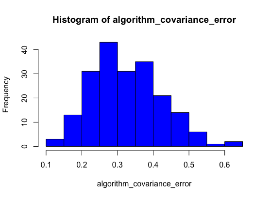
   Figure 1: Distribution of RelErr($S^{*}$, Frob).

   

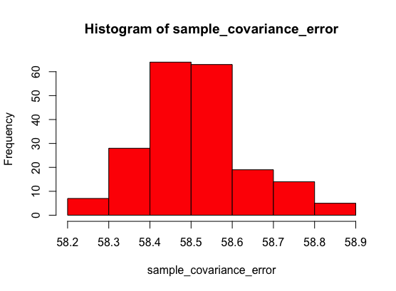
   Figure 2: Distribution of RelErr($\widetilde{\Sigma}_{s}$, Frob).

   The histograms show that $\widetilde{\Sigma}_{s}$ always produces a relative error in the Frobenius norm around $58.5$, while $S^{*}$ always produces a relative error in the Frobenius norm around $0.3$. The average and maximum (over 200 repetitions) relative errors of $S^{*}$ were $0.3246$ and $0.6144$ respectively, with the standard deviation of $0.0979$. The corresponding values for $\widetilde{\Sigma}_{s}$ were $58.5124$, $58.8629$ and $0.1227$. It is clear that in the considered scenario, estimator $S^{*}$ performed noticeably better than the sample covariance $\widetilde{\Sigma}_{s}$.
   In the meanwhile, the following histograms (Figure 4 and 4) show that $S^{*}$ produces smaller relative errors in the operator norm as well. The average and maximum relative errors of $S^{*}$ in the operator norm were $0.2700$ and $0.5324$ respectively, with the standard deviation of $0.0983$. The corresponding values for $\widetilde{\Sigma}_{s}$ were $58.8055$, $59.1579$ and $0.1233$.

   

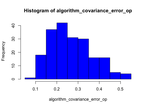
   Figure 3: Distribution of RelErr($S^{*}$, op).

   

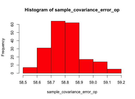
   Figure 4: Distribution of RelErr($\widetilde{\Sigma}_{s}$, op).

2. Spherical Gaussian outliers. Consider the case that the outliers $V_{j}$ are drawn independently from a spherical Gaussian distribution $\mathcal{N}(\mu_{V},\Sigma_{V})$, where $\mu_{V}=(0,\ldots,0)^{T}$, $\Sigma_{V}=\text{diag}(100,\ldots,100)$. In this case, the outliers affect $Z_{j}$ uniformly in all directions. We performed 200 repetitions of the experiment with $\lambda_{1}=3$, $\lambda_{2}=1$, and recorded $S^{*}$, $\widetilde{\Sigma}_{s}$ for each run. Histograms illustrating the distributions of relative errors are shown in Figure 6 and 6:

   

   Figure 5: Distribution of RelErr($S^{*}$, Frob).

   

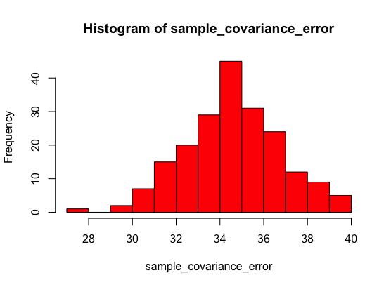
   Figure 6: Distribution of RelErr($\widetilde{\Sigma}_{s}$, Frob).

   The histograms show that $\widetilde{\Sigma}_{s}$ always produces a relative error in the Frobenius norm around $34$, while $S^{*}$ always produces a relative error in the Frobenius norm around $0.3$. The average and maximum (over 200 repetitions) relative errors of $S^{*}$ were $0.2842$ and $0.6346$ respectively, with the standard deviation of $0.1108$. The corresponding values for $\widetilde{\Sigma}_{s}$ were $34.5880$, $39.6758$ and $2.1501$. It is clear that in the considered scenario, estimator $S^{*}$ performed noticeably better than the sample covariance $\widetilde{\Sigma}_{s}$.
   In the meanwhile, the following histograms (Figure 8 and 8) show that $S^{*}$ produces smaller relative errors in the operator norm as well. The average and maximum relative errors of $S^{*}$ in the operator norm were $0.2676$ and $0.6290$ respectively, with the standard deviation of $0.1148$. The corresponding values for $\widetilde{\Sigma}_{s}$ were $22.9255$, $28.2328$ and $1.8791$.

   

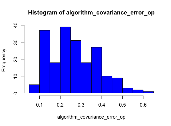
   Figure 7: Distribution of RelErr($S^{*}$, op).

   

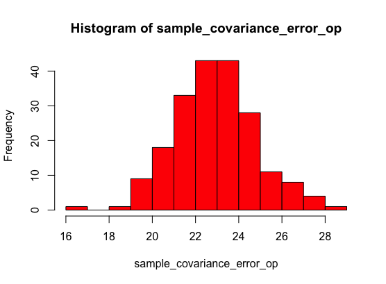
   Figure 8: Distribution of RelErr($\widetilde{\Sigma}_{s}$, op).

3. Outliers that “erase” some observations. Consider the case that the outliers are given as $V_{j}=\beta Z_{j}$ for $j\in J,\beta\in\mathbb{R}$. In this case, the outliers erase (when $\beta=-1$), amplify (when $\beta>0$) or negatively amplify (when $\beta<-1$) some sample points $Z_{j}$. We performed 200 repetitions of the experiment with $\lambda_{1}=\lambda_{2}=0.4$, $\beta=-50$ and recorded $S^{*}$, $\widetilde{\Sigma}_{s}$ for each run. Histograms illustrating the distributions of relative errors are shown in Figure 10 and 10:

   

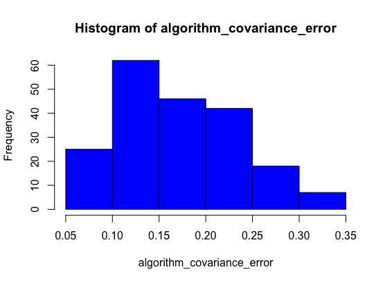
   Figure 9: Distribution of RelErr($S^{*}$, Frob).

   

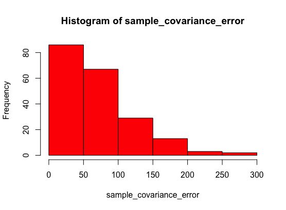
   Figure 10: Distribution of RelErr($\widetilde{\Sigma}_{s}$, Frob).

   The histograms show that $S^{*}$ always produces a relative error in the Frobenius norm around $0.15$, while $\widetilde{\Sigma}_{s}$ produces a relative error in the Frobenius norm around $50$. Note that unlike previous examples, the performance of $\widetilde{\Sigma}_{s}$ is unstable in the current settings, with relative errors raising to $300$ occasionally. The average and maximum (over 200 repetitions) relative errors of $S^{*}$ were $0.1716$ and $0.3383$ respectively, with the standard deviation of $0.0644$. The corresponding values for $\widetilde{\Sigma}_{s}$ were $72.9263$, $263.0925$ and $50.3815$. It is clear that in the considered scenario, estimator $S^{*}$ performed noticeably better than the sample covariance $\widetilde{\Sigma}_{s}$.
   In the meanwhile, the following histograms (Figure 12 and 12) show that $S^{*}$ produces smaller and more stable relative errors in the operator norm as well. The average and maximum relative errors of $S^{*}$ in the operator norm were $0.1652$ and $0.3393$ respectively, with the standard deviation of $0.0680$. The corresponding values for $\widetilde{\Sigma}_{s}$ were $72.7100$, $263.4040$ and $50.8983$.

   

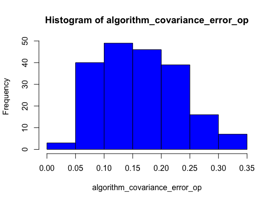
   Figure 11: Distribution of RelErr($S^{*}$, op).

   

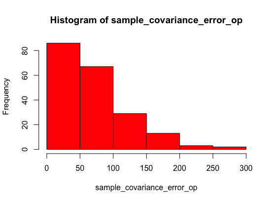
   Figure 12: Distribution of RelErr($\widetilde{\Sigma}_{s}$, op).

4. Outliers in a particular direction. Finally we consider the case that the outliers are all orthogonal (or parallel) to the subspace spanned by the first $M$ principal components of $Z$, where Z is an $n\times d$ matrix with $Z_{j}^{T}$ on each row. We performed 200 repetitions of the experiment with $\lambda_{1}=3$, $\lambda_{2}=1$, $M=1$ (orthogonal case) and recorded $S^{*}$, $\widetilde{\Sigma}_{s}$ for each run. Histograms illustrating the distributions of relative errors are shown in Figure 14 and 14:

   

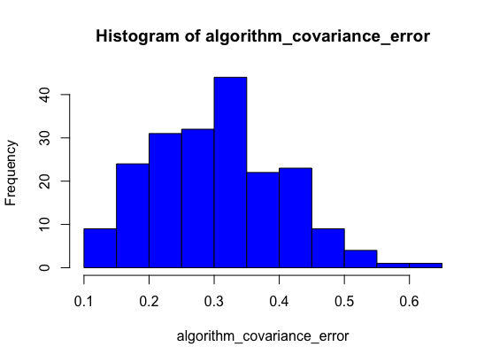
   Figure 13: Distribution of RelErr($S^{*}$, Frob).

   

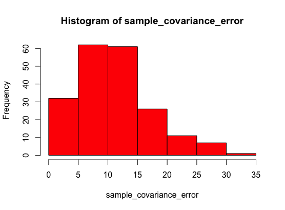
   Figure 14: Distribution of RelErr($\widetilde{\Sigma}_{s}$, Frob).

   The histograms show that $\widetilde{\Sigma}_{s}$ mainly produces a relative error in the Frobenius norm around $10$, while $S^{*}$ always produces a relative error in the Frobenius norm around $0.3$. The average and maximum (over 200 repetitions) relative errors of $S^{*}$ were $0.3038$ and $0.6296$ respectively, with the standard deviation of $0.1021$. The corresponding values for $\widetilde{\Sigma}_{s}$ were $11.1444$, $30.5072$ and $6.2206$. Note that the smallest error produced by $\widetilde{\Sigma}_{s}$ was $0.2930$, which is comparable to the error produced by $S^{*}$. However, the histograms show that the small error produced by $\widetilde{\Sigma}_{s}$ only occurs occasionally, while $S^{*}$ was producing small errors consistently. Therefore, in the considered scenario, we can still conclude that estimator $S^{*}$ performed better than the sample covariance $\widetilde{\Sigma}_{s}$.
   In the meanwhile, the following histograms (Figure 16 and 16) show that $S^{*}$ produces smaller relative errors in the operator norm as well. The average and maximum relative errors of $S^{*}$ in the operator norm were $0.2573$ and $0.5888$ respectively, with the standard deviation of $0.1038$. The corresponding values for $\widetilde{\Sigma}_{s}$ were $11.1985$, $30.6591$ and $6.2528$.

   

   Figure 15: Distribution of RelErr($S^{*}$, op).

   

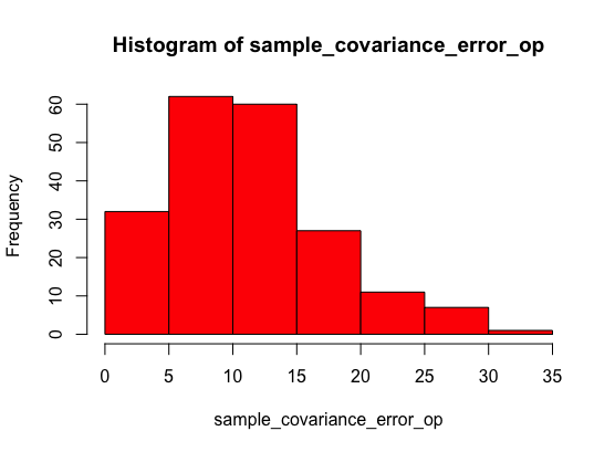
   Figure 16: Distribution of RelErr($\widetilde{\Sigma}_{s}$, op).

Appendix B Proofs ommited from the main exposition

In this section, we present the proofs that were omitted from the main exposition in Section 3.1. We start by introducing some technical tools that will be useful for the proof.

B.1 Technical tools

First, we have the following useful trace duality inequalities for the Frobenius inner product.

Proposition 3.

For any $A,B\in\mathbb{R}^{d_{1}\times d_{2}}$,

$$|\left\langle A,B\right\rangle| \leq \left\|A\right\|_{F}\left\|B\right\|_{F},$$

$$|\left\langle A,B\right\rangle| \leq \left\|A\right\|_{1}\left\|B\right\|.$$

Next, let $L$ be a linear subspace of $\mathbb{R}^{d}$ and $L^{\perp}$ be its orthogonal complement, namely, $L^{\perp}=\big{\{}v\in\mathbb{R}^{d}:\left\langle v,u\right\rangle=0,\forall\,u\in L\big{\}}$. In what follows, $P_{L}$ will stand for the orthogonal projection onto $L$, meaning that $P_{L}\in\mathbb{R}^{d\times d}$ is such that $P_{L}^{2}=P_{L}=P_{L}^{T}$ and $\mathrm{Im}(P_{L})\subseteq L$, where $\mathrm{Im}(P_{L})$ represents the image of $P_{L}$. Given the spectral decomposition of a real symmetric matrix, we have the following proposition:

Proposition 4.

Let $S\in S^{d}(\mathbb{R})$ be a real symmetric matrix with spectral decomposition $S=\sum_{j=1}^{d}\lambda_{j}u_{j}u_{j}^{T}$, where the eigenvalues satisfy $|\lambda_{1}|\geq\cdots\geq|\lambda_{d}|\geq 0$. Denote $L=\mathrm{Im}(S)=\mathrm{span}\left\{u_{j}:\lambda_{j}\neq 0\right\}$. Then $P_{L}=\sum_{j:\lambda_{j}\neq 0}u_{j}u_{j}^{T}$ and $P_{L^{\perp}}=\sum_{j:\lambda_{j}=0}u_{j}u_{j}^{T}$.

Moreover, we will be interested in a linear operator $\mathcal{P}_{L}:\mathbb{R}^{d\times d}\mapsto\mathbb{R}^{d\times d}$ defined as

$$\mathcal{P}_{L}(A):=A-P_{L^{\perp}}AP_{L^{\perp}}.$$ (B.31)

The following lemma provides some results on $\mathcal{P}_{L}(\cdot)$ that will be useful in our proof.

Lemma 3.

Let $L$ be a linear subspace of $\mathbb{R}^{d}$ and $A\in S^{d}(\mathbb{R})$ be an arbitrary real symmetric matrix, then

1. $\left\|\mathcal{P}_{L}(A)\right\|\leq\left\|A\right\|$.

2. $\mathrm{\,rank}(\mathcal{P}_{L}(A))\leq 2\dim(L)$.

Proof.

The proof of this lemma follows straightforward from the definition of $\mathcal{P}_{L}$ and hence omitted here. ∎

The following proposition characterizes the subdifferential of the convex function $A\mapsto\left\|A\right\|_{1}$.

Proposition 5 (Watson (1992)).

Let $A\in S^{d}(\mathbb{R})$ be a symmetric matrix and $A=\sum_{j=1}^{\mathrm{\,rank}(A)}\sigma_{j}u_{j}v_{j}^{T}$ be the singular value decomposition. Denote $L=\mathrm{span}\{u_{1},\ldots,u_{r}\}$, then

$$\partial\left\|A\right\|_{1}=\left\{\sum_{j:\sigma_{j}>0}u_{j}v_{j}^{T}+P_{L^{\perp}}WP_{L^{\perp}}:\left\|W\right\|\leq 1\right\},$$

where $P_{L^{\perp}}$ represents the orthogonal projection onto $L^{\perp}$.

Next, we state some results for the best rank-k approximation. We say that the function ${\left|\kern-1.07639pt\left|\kern-1.07639pt\left|\cdot\right|\kern-1.07639pt\right|\kern-1.07639pt\right|}:\mathbb{R}^{d_{1}\times d_{2}}\mapsto\mathbb{R}$ is a matrix norm if for any scalar $\alpha\in\mathbb{R}$ and any matrices $A,B\in\mathbb{R}^{d_{1}\times d_{2}}$, the following properties are satisfied:

• ${\left|\kern-1.07639pt\left|\kern-1.07639pt\left|\alpha A\right|\kern-1.07639pt\right|\kern-1.07639pt\right|}=|\alpha|{\left|\kern-1.07639pt\left|\kern-1.07639pt\left|A\right|\kern-1.07639pt\right|\kern-1.07639pt\right|}$;

• ${\left|\kern-1.07639pt\left|\kern-1.07639pt\left|A+B\right|\kern-1.07639pt\right|\kern-1.07639pt\right|}\leq{\left|\kern-1.07639pt\left|\kern-1.07639pt\left|A\right|\kern-1.07639pt\right|\kern-1.07639pt\right|}+{\left|\kern-1.07639pt\left|\kern-1.07639pt\left|B\right|\kern-1.07639pt\right|\kern-1.07639pt\right|}$;

• ${\left|\kern-1.07639pt\left|\kern-1.07639pt\left|A\right|\kern-1.07639pt\right|\kern-1.07639pt\right|}\geq 0$, and ${\left|\kern-1.07639pt\left|\kern-1.07639pt\left|A\right|\kern-1.07639pt\right|\kern-1.07639pt\right|}=0$ if and only if $A=0_{d_{1}\times d_{2}}$.

The operator norm $\left\|\cdot\right\|$, the Frobenius norm $\left\|\cdot\right\|_{F}$ and the nuclear norm$\left\|\cdot\right\|_{1}$ introduced in Definition 1 are concrete examples of matrix norms. Given a nonnegative definite matrix $\Sigma$, we say that $\Sigma(k)$ is the best rank-k approximation of $\Sigma$ with respect to the matrix norm ${\left|\kern-1.07639pt\left|\kern-1.07639pt\left|\cdot\right|\kern-1.07639pt\right|\kern-1.07639pt\right|}$, if

$$\Sigma(k)=\mathop{\mbox{argmin}}_{S:\mathrm{\,rank}(S)\leq k}{\left|\kern-1.07639pt\left|\kern-1.07639pt\left|S-\Sigma\right|\kern-1.07639pt\right|\kern-1.07639pt\right|}.$$

The following theorem characterized the best rank-k approximation.

Theorem 8 (Kishore Kumar and Schneider (2017)).

Let $\Sigma\in\mathbb{R}^{d\times d}$ be a nonnegative definite matrix with spectral decomposition $\Sigma=\sum_{j=1}^{d}\lambda_{j}u_{j}u_{j}^{T}$, where the eigenvalues satisfy $\lambda_{1}\geq\cdots\geq\lambda_{d}\geq 0$. Then the matrix $A:=\sum_{j=1}^{k}\lambda_{j}u_{j}u_{j}^{T}$ is the best rank-k approximation of $\Sigma$ in both Frobenius norm and operator norm. Consequently, we have that

$$\min_{S:\mathrm{\,rank}(S)\leq k}\left\|S-\Sigma\right\|=\lambda_{k+1}$$

and

$$\min_{S:\mathrm{\,rank}(S)\leq k}\left\|S-\Sigma\right\|_{F}=\sqrt{\sum_{j=k+1}^{d}\lambda_{j}^{2}}.$$

The following two corollaries will be used in our proof.

Corollary 3.

Let $\Sigma(k)$ be the best rank-k approximation of $\Sigma$ in the operator norm. Then $\left\|\Sigma(k)-\Sigma\right\|\leq\left\|\Sigma\right\|\left(({\mathrm{rk}(\Sigma)}/{k})\wedge\sqrt{{\mathrm{rk}(\Sigma)}/{k}}\right)$ and $\left\|\Sigma(k)-\Sigma\right\|_{F}\leq{\mbox{tr\,}(\Sigma)^{2}}/{k}$.

Proof.

Let $\lambda_{j}(A)$ be the j-th largest eigenvalue of a nonnegative definite matrix, then by Theorem 8,$\left\|\Sigma(k)-\Sigma\right\|\allowbreak=\lambda_{k+1}(\Sigma)$. Moreover, we have that

$$\lambda_{k+1}(\Sigma)\leq\frac{\sum_{j=1}^{k+1}\lambda_{j}(\Sigma)}{k+1}\leq\frac{\mbox{tr\,}(\Sigma)}{k+1}\leq\frac{\mbox{tr\,}(\Sigma)}{k}=\left\|\Sigma\right\|\frac{\mathrm{rk}(\Sigma)}{k}.$$ (B.32)

Note that $\lambda_{k+1}(\Sigma)\leq\sqrt{\left\|\Sigma\right\|}\sqrt{\lambda_{k+1}(\Sigma)}$. Combining this with the previous display, we get another inequality

$$\lambda_{k+1}(\Sigma)\leq\sqrt{\frac{\left\|\Sigma\right\|tr(\Sigma)}{k}}=\left\|\Sigma\right\|\sqrt{\frac{\mathrm{rk}(\Sigma)}{k}}.$$

So we have that $\left\|\Sigma(k)-\Sigma\right\|\leq\left\|\Sigma\right\|\left(({\mathrm{rk}(\Sigma)}/{k})\wedge\sqrt{{\mathrm{rk}(\Sigma)}/{k}}\right)$. To obtain the bound in the Frobenius norm, we note that

$$\left\|\Sigma(k)-\Sigma\right\|_{F}^{2}=\sum_{j\geq k+1}\lambda_{j}(\Sigma)^{2}\leq(\mbox{tr\,}(\Sigma))^{2}\sum_{j\geq k+1}j^{-2}\leq\frac{\mbox{tr\,}(\Sigma)^{2}}{k},$$

where the first inequality follows from (B.32) and the second inequality follows from $\sum_{j\geq k+1}j^{-2}=\sum_{j\geq k+1}j^{-1}(j+1)^{-1}\allowbreak=1/(k+1).$ ∎

Remark 6.

It is easy to see that ${\mathrm{rk}(\Sigma)}/{k}\leq\sqrt{{\mathrm{rk}(\Sigma)}/{k}}$ if and only if $\mathrm{rk}(\Sigma)\leq k$, so when $\Sigma$ has low effective rank, i.e. $\mathrm{rk}(\Sigma)\leq k$, the upper bound becomes

$$\left\|\Sigma(k)-\Sigma\right\|\leq\frac{\left\|\Sigma\right\|\mathrm{rk}(\Sigma)}{k}.$$

Corollary 4.

Let $\Sigma(k)$ be the best rank-k approximation of $\Sigma$ in the operator norm defined in Theorem 8, and $L(k):=\mathrm{Im}(\Sigma(k))$. Then $\mathcal{P}_{L(k)}(\Sigma)=\Sigma(k)$.

Proof.

By Theorem 8, $\Sigma(k)$ has spectral decomposition $\Sigma(k)=\sum_{j=1}^{d}\lambda_{j}u_{j}u_{j}^{T}$ with $\lambda_{k+1}=\cdots=\lambda_{d}=0$. Then Proposition 4 implies that $P_{L(k)^{\perp}}=\sum_{j=k+1}^{d}u_{j}u_{j}^{T}$. Therefore,

$$\mathcal{P}_{L(k)}(\Sigma)=\Sigma-P_{L(k)^{\perp}}\Sigma P_{L(k)^{\perp}}=\sum_{j=1}^{d}\lambda_{j}u_{j}u_{j}^{T}-\sum_{j=k+1}^{d}\lambda_{j}u_{j}u_{j}^{T}\\ =\sum_{j=1}^{k}\lambda_{j}u_{j}u_{j}^{T}=\Sigma(k).$$

∎

B.2 Proof of Theorem 1

To simplify the notations, we denote $N:=n(n-1)$. Let

$$F(S,\mathbf{U_{I_{n}^{2}}})=\frac{1}{N}\sum_{i\neq j}\left\|\widetilde{Y}_{i,j}\widetilde{Y}_{i,j}^{T}-S-\sqrt{N}U_{i,j}\right\|^{2}_{\mathrm{F}}\\ +\lambda_{1}\left\|S\right\|_{1}+\lambda_{2}\sum_{i\neq j}\left\|U_{i,j}\right\|_{1}.$$ (B.33)

The function $F$ is convex, and we have that

$$\partial F(S,\boldsymbol{U_{I_{n}^{2}}})=\begin{pmatrix}-\frac{2}{N}\sum_{i\neq j}(\widetilde{Y}_{i,j}\widetilde{Y}_{i,j}^{T}-S-\sqrt{N}U_{i,j})\\ -\frac{2}{N}\sqrt{N}(\widetilde{Y}_{1,2}\widetilde{Y}_{1,2}^{T}-S-\sqrt{N}U_{1,2})\\ \vdots\\ -\frac{2}{N}\sqrt{N}(\widetilde{Y}_{n,n-1}\widetilde{Y}_{n,n-1}^{T}-S-\sqrt{N}U_{n,n-1})\end{pmatrix}+\begin{pmatrix}\lambda_{1}\partial\left\|S\right\|_{1}\\ \lambda_{2}\partial\left\|U_{1,2}\right\|_{1}\\ \vdots\\ \lambda_{2}\partial\left\|U_{n,n-1}\right\|_{1}\end{pmatrix}$$ (B.34)

where $\partial\left\|A\right\|_{1}$ represents the subdifferential of $\left\|\cdot\right\|_{1}$ at $A$. Note that for any symmetric matrices $S,U_{1,2},\ldots,U_{n,n-1}$, the directional derivative of $F$ at the point $\big{(}\widehat{S}_{\lambda},\widehat{U}_{1,2},\ldots\allowbreak,\allowbreak\widehat{U}_{n,n-1}\big{)}$ in the direction $\big{(}S-\widehat{S}_{\lambda},U_{1,2}-\widehat{U}_{1,2},\ldots\allowbreak,\allowbreak U_{n,n-1}-\widehat{U}_{n,n-1}\big{)}$ is nonnegative. In particular, we consider an arbitrary S and $U_{1,2}:=\widetilde{U}_{1,2}^{*},\ldots,U_{n,n-1}:=\widetilde{U}_{n,n-1}^{*}$. By the necessary condition of the minima, there exist $\widehat{V}\in\partial\|\widehat{S}_{\lambda}\|_{1},\ \widehat{W}_{1,2}\in\partial\|\widehat{U}_{1,2}\|_{1},\ldots,\widehat{W}_{n,n-1}\in\partial\|\widehat{U}_{n,n-1}\|_{1}$ such that

$$\left\langle\partial F(\widehat{S},\mathbf{\widehat{U}_{I_{n}^{2}}}),(S-\widehat{S}_{\lambda};\mathbf{\widetilde{U}_{I_{n}^{2}}^{*}}-\mathbf{\widehat{U}_{I_{n}^{2}}})\right\rangle=\\ -\frac{2}{N}\sum_{i\neq j}\left\langle\widetilde{Y}_{i,j}\widetilde{Y}_{i,j}^{T}-\widehat{S}_{\lambda}-\sqrt{N}\widehat{U}_{i,j},S-\widehat{S}_{\lambda}+\sqrt{N}(\widetilde{U}_{i,j}^{*}-\widehat{U}_{i,j})\right\rangle\\ +\lambda_{1}\left\langle\widehat{V},S-\widehat{S}_{\lambda}\right\rangle+\lambda_{2}\sum_{i\neq j}\left\langle\widehat{W}_{i,j},\widetilde{U}_{i,j}^{*}-\widehat{U}_{i,j}\right\rangle\geq 0.$$

For any choice of $V\in\partial\left\|S\right\|_{1},\ W_{1,2}\in\partial\left\|\widetilde{U}_{1,2}^{*}\right\|_{1},\ldots\allowbreak,\allowbreak W_{n,n-1}\in\partial\left\|\widetilde{U}_{n,n-1}^{*}\right\|_{1}$, by the monotonicity of subgradients we deduce that

$$\left\langle V-\widehat{V},S-\widehat{S}_{\lambda}\right\rangle\geq 0,$$

$$\left\langle W_{i,j}-\widehat{W}_{i,j},\widetilde{U}_{i,j}^{*}-\widehat{U}_{i,j}\right\rangle\geq 0,\quad(i,j)\in I_{n}^{2}.$$

Hence the previous display implies that

$$\frac{2}{N}\sum_{i\neq j}\left\langle\widetilde{Y}_{i,j}\widetilde{Y}_{i,j}^{T}-\widehat{S}_{\lambda}-\sqrt{N}\widehat{U}_{i,j},S-\widehat{S}_{\lambda}+\sqrt{N}(\widetilde{U}_{i,j}^{*}-\widehat{U}_{i,j})\right\rangle\\ \leq\lambda_{1}\left\langle V,S-\widehat{S}_{\lambda}\right\rangle+\lambda_{2}\sum_{i\neq j}\left\langle W_{i,j},\widetilde{U}_{i,j}^{*}-\widehat{U}_{i,j}\right\rangle,$$

which is equivalent to

$$\frac{2}{N}\sum_{i\neq j}\left\langle\Sigma-\widehat{S}_{\lambda}+\sqrt{N}(\widetilde{U}_{i,j}^{*}-\widehat{U}_{i,j}),S-\widehat{S}_{\lambda}+\sqrt{N}(\widetilde{U}_{i,j}^{*}-\widehat{U}_{i,j})\right\rangle\\ \leq-\lambda_{1}\left\langle V,\widehat{S}_{\lambda}-S\right\rangle-\lambda_{2}\sum_{i\neq j}\left\langle W_{i,j},\widehat{U}_{i,j}-\widetilde{U}_{i,j}^{*}\right\rangle\\ -2\left\langle\frac{1}{N}\sum_{i\neq j}\widetilde{X}_{i,j}-\Sigma,S-\widehat{S}_{\lambda}\right\rangle-\frac{2}{\sqrt{N}}\sum_{i\neq j}\left\langle\widetilde{X}_{i,j}-\Sigma,\widetilde{U}_{i,j}^{*}-\widehat{U}_{i,j}\right\rangle,$$ (B.35)

where $\widetilde{X}_{i,j}=\widetilde{Z}_{i,j}\widetilde{Z}_{i,j}^{T}$. We will bound (B.35) in two cases.
Case 1: Assume that

$$\frac{2}{N}\sum_{i\neq j}\Big{\langle}{\Sigma-\widehat{S}_{\lambda}+\sqrt{N}(\widetilde{U}_{i,j}^{*}-\widehat{U}_{i,j})},{S-\widehat{S}_{\lambda}+\sqrt{N}(\widetilde{U}_{i,j}^{*}-\widehat{U}_{i,j})}\geq 0.$$

Applying the law of cosines, $2\left\langle A,B\right\rangle=\left\|A\right\|_{F}^{2}+\left\|B\right\|_{F}^{2}-\left\|A-B\right\|_{F}^{2}$, $\forall A,B\in\mathbb{R}^{d\times d}$, to the left hand side of (B.35), we get that

$$\frac{1}{N}\sum_{i\neq j}\left\|\Sigma-\widehat{S}_{\lambda}+\sqrt{N}(\widetilde{U}_{i,j}^{*}-\widehat{U}_{i,j})\right\|_{F}^{2}+\frac{1}{N}\sum_{i\neq j}\left\|S-\widehat{S}_{\lambda}+\sqrt{N}(\widetilde{U}_{i,j}^{*}-\widehat{U}_{i,j})\right\|_{F}^{2}\\ \leq\left\|\Sigma-S\right\|_{F}^{2}+2\left\langle\frac{1}{N}\sum_{i\neq j}\widetilde{X}_{i,j}-\Sigma,\widehat{S}_{\lambda}-S\right\rangle+\frac{2}{\sqrt{N}}\sum_{i\neq j}\left\langle\widetilde{X}_{i,j}-\Sigma,\widehat{U}_{i,j}-\widetilde{U}_{i,j}^{*}\right\rangle\\ -\lambda_{1}\left\langle V,\widehat{S}_{\lambda}-S\right\rangle-\lambda_{2}\sum_{i\neq j}\left\langle W_{i,j},\widehat{U}_{i,j}-\widetilde{U}_{i,j}^{*}\right\rangle.$$ (B.36)

We will now analyze the terms on the right-hand side of equation (B.36) one by one. First, let $S=\sum_{j=1}^{\mathrm{\,rank}(S)}\sigma_{j}(S)u_{j}v_{j}^{T}$ be the singular value decomposition of $S$, where $\sigma_{j}(S)$ is the j-th largest singular value of $S$. Then we can represent any $V\in\partial\left\|S\right\|_{1}$ by $V=\sum_{j=1}^{\mathrm{\,rank}(S)}u_{j}v_{j}^{T}+P_{L^{\perp}}WP_{L^{\perp}}$ for some $\left\|W\right\|\leq 1$, where $L=\text{span}\{u_{1},\ldots,u_{\mathrm{\,rank}(S)}\}$. From this representation, we have that $\mathcal{P}_{L}(V)=V-P_{L^{\perp}}VP_{L^{\perp}}=\sum_{j=1}^{\mathrm{\,rank}(S)}u_{j}v_{j}^{T}$, and

$$-\left\langle V,\widehat{S}_{\lambda}-S\right\rangle =-\left\langle\mathcal{P}_{L}(V),\widehat{S}_{\lambda}-S\right\rangle-\left\langle P_{L^{\perp}}VP_{L^{\perp}},\widehat{S}_{\lambda}-S\right\rangle$$

$$=-\left\langle\mathcal{P}_{L}(V),\widehat{S}_{\lambda}-S\right\rangle-\left\langle W,P_{L^{\perp}}\widehat{S}_{\lambda}P_{L^{\perp}}\right\rangle$$

$$\leq\left|\left\langle\mathcal{P}_{L}(V),\widehat{S}_{\lambda}-S\right\rangle\right|-\left\|P_{L^{\perp}}\widehat{S}_{\lambda}P_{L^{\perp}}\right\|_{1}$$

$$\leq\left\|\mathcal{P}_{L}(V)\right\|_{F}\left\|\widehat{S}_{\lambda}-S\right\|_{F}-\left\|P_{L^{\perp}}\widehat{S}_{\lambda}P_{L^{\perp}}\right\|_{1}$$

$$=\sqrt{\mathrm{\,rank}(S)}\left\|\widehat{S}_{\lambda}-S\right\|_{F}-\left\|P_{L^{\perp}}\widehat{S}_{\lambda}P_{L^{\perp}}\right\|_{1},$$ (B.37)

where we chose $W$ such that $\left\langle W,P_{L^{\perp}}\widehat{S}_{\lambda}P_{L^{\perp}}\right\rangle\allowbreak=\left\|P_{L^{\perp}}\widehat{S}_{\lambda}P_{L^{\perp}}\right\|_{1}$. Similarly, let $L_{i,j}$ be the image of $\widetilde{U}^{*}_{i,j}\allowbreak,\allowbreak(i,j)\in I_{n}^{2}$, then for properly chosen $W_{1,2}\in\partial\left\|\widetilde{U}^{*}_{1,2}\right\|_{1},\ldots\allowbreak,\allowbreak W_{n,n-1}\in\partial\left\|\widetilde{U}^{*}_{n,n-1}\right\|_{1}$, we have that

$$-\sum_{i\neq j}\left\langle W_{i,j},\widehat{U}_{i,j}-\widetilde{U}_{i,j}^{*}\right\rangle\\ \leq-\sum_{i\neq j}\left\|P_{L_{i,j}^{\perp}}\widehat{U}_{i,j}P_{L_{i,j}^{\perp}}\right\|_{1}+\sum_{i\neq j}\left|\left\langle\mathcal{P}_{L_{i,j}}(W_{i,j}),\widehat{U}_{i,j}-\widetilde{U}^{*}_{i,j}\right\rangle\right|\\ \leq\sum_{i\neq j}\sqrt{\mathrm{\,rank}(\widetilde{U}_{i,j}^{*})}\left\|\widehat{U}_{i,j}-\widetilde{U}^{*}_{i,j}\right\|_{F}-\sum_{i\neq j}\left\|P_{L_{i,j}^{\perp}}\widehat{U}_{i,j}P_{L_{i,j}^{\perp}}\right\|_{1}\\ \leq\sum_{(i,j)\in\widetilde{J}}\sqrt{2}\left\|\widehat{U}_{i,j}-\widetilde{U}^{*}_{i,j}\right\|_{F}-\sum_{i\neq j}\left\|P_{L_{i,j}^{\perp}}\widehat{U}_{i,j}P_{L_{i,j}^{\perp}}\right\|_{1},$$ (B.38)

where we used the fact that $\mathrm{\,rank}(\widetilde{U}^{*}_{i,j})\leq 2$, and $\widetilde{U}^{*}_{i,j}=0$, $L_{i,j}=\{0\}$ for $(i,j)\notin\widetilde{J}$. Next, we denote $\Delta:=\frac{1}{N}\sum_{i\neq j}\widetilde{X}_{i,j}-\Sigma$ and recall the linear operator defined in (B.31):

$$\mathcal{P}(A)=A-P_{L^{\perp}}AP_{L^{\perp}}.$$

It is easy to check that $\mathcal{P}_{L}(\Delta)=P_{L^{\perp}}\Delta P_{L}+P_{L}\Delta$, which implies $\mathrm{\,rank}(\mathcal{P}_{L}(\Delta))\leq 2\mathrm{\,rank}(S)$. Therefore,

$$\left\langle\Delta,\widehat{S}_{\lambda}-S\right\rangle=\left\langle\mathcal{P}_{L}(\Delta),\widehat{S}_{\lambda}-S\right\rangle+\left\langle P_{L^{\perp}}\Delta P_{L^{\perp}},\widehat{S}_{\lambda}-S\right\rangle\\ =\left\langle\mathcal{P}_{L}(\Delta),\widehat{S}_{\lambda}-S\right\rangle+\left\langle\Delta,P_{L^{\perp}}(\widehat{S}_{\lambda}-S)P_{L^{\perp}}\right\rangle\\ \leq\left\|\mathcal{P}_{L}(\Delta)\right\|_{F}\left\|\widehat{S}_{\lambda}-S\right\|_{F}+\left\|\Delta\right\|\left\|P_{L^{\perp}}\widehat{S}_{\lambda}P_{L^{\perp}}\right\|_{1}\\ \leq\sqrt{\mathrm{\,rank}(\mathcal{P}_{L}(\Delta))}\left\|\mathcal{P}_{L}(\Delta)\right\|\left\|\widehat{S}_{\lambda}-S\right\|_{F}+\left\|\Delta\right\|\left\|P_{L^{\perp}}\widehat{S}_{\lambda}P_{L^{\perp}}\right\|_{1}\\ \leq\sqrt{2\mathrm{\,rank}(S)}\left\|\Delta\right\|\left\|\widehat{S}_{\lambda}-S\right\|_{F}+\left\|\Delta\right\|\left\|P_{L^{\perp}}\widehat{S}_{\lambda}P_{L^{\perp}}\right\|_{1},$$ (B.39)

where the last inequality follows from the bound $\left\|\mathcal{P}_{L}(\Delta)\right\|\leq\left\|\Delta\right\|$. Finally, it is easy to see that

$$\sum_{i\neq j}\left\langle\widetilde{X}_{i,j}-\Sigma,\widehat{U}_{i,j}-\widetilde{U}^{*}_{i,j}\right\rangle=\sum_{i\neq j}\left\langle\mathcal{P}_{L_{i,j}}(\widetilde{X}_{i,j}-\Sigma),\widehat{U}_{i,j}-\widetilde{U}^{*}_{i,j}\right\rangle\\ +\sum_{i\neq j}\left\langle P_{L_{i,j}^{\perp}}(\widetilde{X}_{i,j}-\Sigma)P_{L_{i,j}^{\perp}},\widehat{U}_{i,j}-\widetilde{U}^{*}_{i,j}\right\rangle\\ \leq\sum_{i\neq j}\left\|\mathcal{P}_{L_{i,j}}(\widetilde{X}_{i,j}-\Sigma)\right\|_{F}\left\|\widehat{U}_{i,j}-\widetilde{U}^{*}_{i,j}\right\|_{F}+\sum_{i\neq j}\left\|\widetilde{X}_{i,j}-\Sigma\right\|\left\|P_{L_{i,j}^{\perp}}\widehat{U}_{i,j}P_{L_{i,j}^{\perp}}\right\|_{1}\\ \leq\sum_{(i,j)\in\widetilde{J}}\sqrt{2\mathrm{\,rank}(\widetilde{U}^{*}_{i,j})}\left\|\widetilde{X}_{i,j}-\Sigma\right\|\left\|\widehat{U}_{i,j}-\widetilde{U}^{*}_{i,j}\right\|_{F}+\sum_{i\neq j}\left\|\widetilde{X}_{i,j}-\Sigma\right\|\left\|P_{L_{i,j}^{\perp}}\widehat{U}_{i,j}P_{L_{i,j}^{\perp}}\right\|_{1}\\ \leq\sum_{(i,j)\in\widetilde{J}}\sqrt{4}\left\|\widetilde{X}_{i,j}-\Sigma\right\|\left\|\widehat{U}_{i,j}-\widetilde{U}^{*}_{i,j}\right\|_{F}+\sum_{i\neq j}\left\|\widetilde{X}_{i,j}-\Sigma\right\|\left\|P_{L_{i,j}^{\perp}}\widehat{U}_{i,j}P_{L_{i,j}^{\perp}}\right\|_{1}.$$ (B.40)

Combining inequalities (B.2, B.38, B.39, B.40) with (B.36), we deduce that

$$\frac{1}{N}\sum_{i\neq j}\left\|\Sigma-\widehat{S}_{\lambda}+\sqrt{N}(\widetilde{U}_{i,j}^{*}-\widehat{U}_{i,j})\right\|_{F}^{2}+\frac{1}{N}\sum_{i\neq j}\left\|S-\widehat{S}_{\lambda}+\sqrt{N}(\widetilde{U}_{i,j}^{*}-\widehat{U}_{i,j})\right\|_{F}^{2}\\ \leq\left\|\Sigma-S\right\|_{F}^{2}+2\left(\sqrt{2\mathrm{\,rank}(S)}\left\|\Delta\right\|\left\|\widehat{S}_{\lambda}-S\right\|_{F}+\left\|\Delta\right\|\left\|P_{L^{\perp}}\widehat{S}_{\lambda}P_{L^{\perp}}\right\|_{1}\right)\\ +\frac{2}{\sqrt{N}}\left(\sum_{(i,j)\in\widetilde{J}}\sqrt{4}\left\|\widetilde{X}_{i,j}-\Sigma\right\|\left\|\widehat{U}_{i,j}-\widetilde{U}^{*}_{i,j}\right\|_{F}+\sum_{i\neq j}\left\|\widetilde{X}_{i,j}-\Sigma\right\|\left\|P_{L_{i,j}^{\perp}}\widehat{U}_{i,j}P_{L_{i,j}^{\perp}}\right\|_{1}\right)\\ +\lambda_{1}\Big{(}\sqrt{\mathrm{\,rank}(S)}\left\|\widehat{S}_{\lambda}-S\right\|_{F}-\left\|P_{L^{\perp}}\widehat{S}_{\lambda}P_{L^{\perp}}\right\|_{1}\Big{)}\\ +\lambda_{2}\left(\sum_{(i,j)\in\widetilde{J}}\sqrt{2}\left\|\widehat{U}_{i,j}-\widetilde{U}^{*}_{i,j}\right\|_{F}-\sum_{i\neq j}\left\|P_{L_{i,j}^{\perp}}\widehat{U}_{i,j}P_{L_{i,j}^{\perp}}\right\|_{1}\right),$$

which is equivalent to

$$\frac{1}{N}\sum_{i\neq j}\left\|\Sigma-\widehat{S}_{\lambda}+\sqrt{N}(\widetilde{U}_{i,j}^{*}-\widehat{U}_{i,j})\right\|_{F}^{2}+\frac{1}{N}\sum_{i\neq j}\left\|S-\widehat{S}_{\lambda}+\sqrt{N}(\widetilde{U}_{i,j}^{*}-\widehat{U}_{i,j})\right\|_{F}^{2}\\ +\left(\lambda_{1}-2\left\|\Delta\right\|\right)\left\|P_{L^{\perp}}\widehat{S}_{\lambda}P_{L^{\perp}}\right\|_{1}+\left(\lambda_{2}-\frac{2}{\sqrt{N}}\max_{i\neq j}\left\|\widetilde{X}_{i,j}-\Sigma\right\|\right)\left\|P_{L_{i,j}^{\perp}}\widehat{U}_{i,j}P_{L_{i,j}^{\perp}}\right\|_{1}\\ \leq\left\|\Sigma-S\right\|_{F}^{2}+\left(2\sqrt{2\mathrm{\,rank}(S)}\left\|\Delta\right\|+\lambda_{1}\sqrt{\mathrm{\,rank}(S)}\right)\left\|\widehat{S}_{\lambda}-S\right\|_{F}\\ +\sum_{(i,j)\in\widetilde{J}}\left(\frac{4}{\sqrt{N}}\left\|\widetilde{X}_{i,j}-\Sigma\right\|+\lambda_{2}\sqrt{2}\right)\left\|\widehat{U}_{i,j}-\widetilde{U}^{*}_{i,j}\right\|_{F}.$$ (B.41)

Now consider the event

$$\mathcal{E}_{1}:=\left\{\lambda_{1}\geq 2\left\|\Delta\right\|,\lambda_{2}\geq\frac{3}{\sqrt{N}}\max_{i\neq j}\left\|\widetilde{X}_{i,j}-\Sigma\right\|\right\}.$$

We will derive a bound for $\left\|\widehat{S}_{\lambda}-\Sigma\right\|_{F}^{2}+\sum_{i\neq j}\left\|\widehat{U}_{i,j}-\widetilde{U}^{*}_{i,j}\right\|_{F}^{2}$ on $\mathcal{E}_{1}$. Applying the identity $\left\|A+B\right\|_{F}^{2}=\left\|A\right\|_{F}^{2}+\left\|B\right\|_{F}^{2}+2\left\langle A,B\right\rangle$ to the the left-hand side of (B.41), we get that on the event $\mathcal{E}_{1}$,

$$\left\|\Sigma-\widehat{S}_{\lambda}\right\|_{F}^{2}+\left\|S-\widehat{S}_{\lambda}\right\|_{F}^{2}+2\sum_{i\neq j}\left\|\widetilde{U}^{*}_{i,j}-\widehat{U}_{i,j}\right\|_{F}^{2}\\ \leq\left\|\Sigma-S\right\|_{F}^{2}+\left(2\sqrt{2\mathrm{\,rank}(S)}\left\|\Delta\right\|+\lambda_{1}\sqrt{\mathrm{\,rank}(S)}\right)\left\|\widehat{S}_{\lambda}-S\right\|_{F}\\ +\frac{2}{\sqrt{N}}\sum_{i\neq j}\left\langle\Sigma-\widehat{S}_{\lambda},\widetilde{U}^{*}_{i,j}-\widehat{U}_{i,j}\right\rangle+\frac{2}{\sqrt{N}}\sum_{i\neq j}\left\langle S-\widehat{S}_{\lambda},\widetilde{U}^{*}_{i,j}-\widehat{U}_{i,j}\right\rangle\\ +\sum_{(i,j)\in\widetilde{J}}\left(\frac{4}{\sqrt{N}}\left\|\widetilde{X}_{ij}-\Sigma\right\|+\lambda_{2}\sqrt{2}\right)\left\|\widehat{U}_{i,j}-\widetilde{U}^{*}_{i,j}\right\|_{F}.$$ (B.42)

We now bound the inner product terms on the right-hand side. First, combining inequalities (B.2, B.38, B.39, B.40) with (B.35), we deduce the following bound:

$$\frac{2}{N}\sum_{i\neq j}\left\langle\Sigma-\widehat{S}_{\lambda}+\sqrt{N}(\widetilde{U}_{i,j}^{*}-\widehat{U}_{i,j}),S-\widehat{S}_{\lambda}+\sqrt{N}(\widetilde{U}_{i,j}^{*}-\widehat{U}_{i,j})\right\rangle\\ +\left(\lambda_{1}-2\left\|\Delta\right\|\right)\left\|P_{L^{\perp}}\widehat{S}_{\lambda}P_{L^{\perp}}\right\|_{1}+\left(\lambda_{2}-\frac{2}{\sqrt{N}}\max_{i\neq j}\left\|\widetilde{X}_{i,j}-\Sigma\right\|\right)\left\|P_{L_{i,j}^{\perp}}\widehat{U}_{i,j}P_{L_{i,j}^{\perp}}\right\|_{1}\\ \leq\left(2\sqrt{2\mathrm{\,rank}(S)}\left\|\Delta\right\|+\lambda_{1}\sqrt{\mathrm{\,rank}(S)}\right)\left\|\widehat{S}_{\lambda}-S\right\|_{F}\\ +\sum_{(i,j)\in\widetilde{J}}\left(\frac{4}{\sqrt{N}}\left\|\widetilde{X}_{i,j}-\Sigma\right\|+\lambda_{2}\sqrt{2}\right)\left\|\widehat{U}_{i,j}-\widetilde{U}^{*}_{i,j}\right\|_{F}.$$ (B.43)

On the event $\mathcal{E}_{1}$ along with the assumption that

$$\frac{2}{N}\sum_{i\neq j}\Big{\langle}{\Sigma-\widehat{S}_{\lambda}+\sqrt{N}(\widetilde{U}_{i,j}^{*}-\widehat{U}_{i,j})},\\ {S-\widehat{S}_{\lambda}+\sqrt{N}(\widetilde{U}_{i,j}^{*}-\widehat{U}_{i,j})}\geq 0.$$

(B.43) implies that

$$\frac{1}{3}\lambda_{2}\left\|P_{L_{i,j}^{\perp}}\widehat{U}_{i,j}P_{L_{i,j}^{\perp}}\right\|_{1}\leq\left(2\sqrt{2\mathrm{\,rank}(S)}\left\|\Delta\right\|+\lambda_{1}\sqrt{\mathrm{\,rank}(S)}\right)\left\|\widehat{S}_{\lambda}-S\right\|_{F}\\ +\sum_{(i,j)\in\widetilde{J}}\left(\frac{4}{\sqrt{N}}\left\|\widetilde{X}_{i,j}-\Sigma\right\|+\lambda_{2}\sqrt{2}\right)\left\|\widehat{U}_{i,j}-\widetilde{U}^{*}_{i,j}\right\|_{F}.$$

Recall that $L_{i,j}=\{0\}$ for any $(i,j)\notin\widetilde{J}$, hence

$$\lambda_{2}\sum_{(i,j)\notin\widetilde{J}}\left\|P_{L_{i,j}^{\perp}}\widehat{U}_{i,j}P_{L_{i,j}^{\perp}}\right\|_{1}\\ =\lambda_{2}\sum_{(i,j)\notin\widetilde{J}}\left\|P_{L_{i,j}^{\perp}}\left(\widehat{U}_{i,j}-\widetilde{U}_{i,j}^{*}\right)P_{L_{i,j}^{\perp}}\right\|_{1}=\lambda_{2}\sum_{(i,j)\notin\widetilde{J}}\left\|\widehat{U}_{i,j}-\widetilde{U}^{*}_{i,j}\right\|_{1}\\ \leq 3\left(2\sqrt{2\mathrm{\,rank}(S)}\left\|\Delta\right\|+\lambda_{1}\sqrt{\mathrm{\,rank}(S)}\right)\left\|\widehat{S}_{\lambda}-S\right\|_{F}\\ +3\sum_{(i,j)\in\widetilde{J}}\left(\frac{4}{\sqrt{N}}\left\|\widetilde{X}_{i,j}-\Sigma\right\|+\lambda_{2}\sqrt{2}\right)\left\|\widehat{U}_{i,j}-\widetilde{U}^{*}_{i,j}\right\|_{F}.$$ (B.44)

Next, we can estimate $\sum_{(i,j)\notin\widetilde{J}}\left|\left\langle\widehat{S}_{\lambda}-S,\widehat{U}_{i,j}-\widetilde{U}^{*}_{i,j}\right\rangle\right|$ as follows:

$$\quad\sum_{(i,j)\notin\widetilde{J}}\left|\left\langle\widehat{S}_{\lambda}-S,\widehat{U}_{i,j}-\widetilde{U}^{*}_{i,j}\right\rangle\right|\leq\left\|\widehat{S}_{\lambda}-S\right\|\sum_{(i,j)\notin\widetilde{J}}\left\|\widehat{U}_{i,j}-\widetilde{U}^{*}_{i,j}\right\|_{1}$$

$$\leq\frac{3\left\|\widehat{S}_{\lambda}-S\right\|}{\lambda_{2}}\Bigg{[}\left(2\sqrt{2\mathrm{\,rank}(S)}\left\|\Delta\right\|+\lambda_{1}\sqrt{\mathrm{\,rank}(S)}\right)\left\|\widehat{S}_{\lambda}-S\right\|_{F}$$

$$\qquad\qquad\qquad+\sum_{(i,j)\in\widetilde{J}}\left(\frac{4}{\sqrt{N}}\left\|\widetilde{X}_{i,j}-\Sigma\right\|+\lambda_{2}\sqrt{2}\right)\left\|\widehat{U}_{i,j}-\widetilde{U}^{*}_{i,j}\right\|_{F}\Bigg{]}$$

$$\leq 3\left\|\widehat{S}_{\lambda}-S\right\|\left[(\sqrt{2}+1)\sqrt{\mathrm{\,rank}(S)}\frac{\lambda_{1}}{\lambda_{2}}\left\|\widehat{S}_{\lambda}-S\right\|_{F}+\Big{(}\frac{4}{3}+\sqrt{2}\Big{)}\sum_{(i,j)\in\widetilde{J}}\left\|\widehat{U}_{i,j}-\widetilde{U}^{*}_{i,j}\right\|_{F}\right],$$ (B.45)

where the last inequality holds on event $\mathcal{E}_{1}$. This implies that

$$\frac{2}{\sqrt{N}}\sum_{i\neq j}\left\langle S-\widehat{S}_{\lambda},\widetilde{U}^{*}_{i,j}-\widehat{U}_{i,j}\right\rangle\leq\frac{2}{\sqrt{N}}\sum_{(i,j)\in\widetilde{J}}\left\langle S-\widehat{S}_{\lambda},\widetilde{U}^{*}_{i,j}-\widehat{U}_{i,j}\right\rangle+\frac{6}{\sqrt{N}}\left\|\widehat{S}_{\lambda}-S\right\|\\ \times\Bigg{[}(\sqrt{2}+1)\sqrt{\mathrm{\,rank}(S)}\frac{\lambda_{1}}{\lambda_{2}}\left\|\widehat{S}_{\lambda}-S\right\|_{F}+\Big{(}\frac{4}{3}+\sqrt{2}\Big{)}\sum_{(i,j)\in\widetilde{J}}\left\|\widehat{U}_{i,j}-\widetilde{U}^{*}_{i,j}\right\|_{F}\Bigg{]}\\ \leq 2\cdot\frac{\left\|\widehat{S}_{\lambda}-S\right\|_{F}}{{2}}\cdot 2\frac{1}{\sqrt{N}}\sqrt{\left|\widetilde{J}\right|}\sqrt{\sum_{(i,j)\in\widetilde{J}}\left\|\widehat{U}_{i,j}-\widetilde{U}^{*}_{i,j}\right\|_{F}^{2}}+(6\sqrt{2}+6)\frac{\lambda_{1}}{\lambda_{2}}\sqrt{\frac{\mathrm{\,rank}(S)}{N}}\left\|\widehat{S}_{\lambda}-S\right\|_{F}^{2}\\ +2\cdot\frac{\left\|\widehat{S}_{\lambda}-S\right\|_{F}}{{2}}\cdot(8+6\sqrt{2})\frac{1}{\sqrt{N}}\sqrt{\left|\widetilde{J}\right|}\sqrt{\sum_{(i,j)\in\widetilde{J}}\left\|\widehat{U}_{i,j}-\widetilde{U}^{*}_{i,j}\right\|_{F}^{2}}\\ \leq\left[(6\sqrt{2}+6)\sqrt{\frac{\mathrm{\,rank}(S)}{N}}\frac{\lambda_{1}}{\lambda_{2}}+\frac{1}{2}\right]\left\|\widehat{S}_{\lambda}-S\right\|_{F}^{2}+\left[4+(6\sqrt{2}+8)^{2}\right]\frac{|\widetilde{J}|}{N}\sum_{(i,j)\in\widetilde{J}}\left\|\widehat{U}_{i,j}-\widetilde{U}^{*}_{i,j}\right\|_{F}^{2},$$ (B.46)

where the second inequality follows from the fact that $\left\|A\right\|\leq\left\|A\right\|_{F}$ for any symmetric matrix A, and the last inequality follows from the fact that $2ab\leq a^{2}+b^{2}$ for any real numbers $a,b$.
Similarly, we deduce that

$$\quad\frac{2}{\sqrt{N}}\sum_{i\neq j}\left\langle\Sigma-\widehat{S}_{\lambda},\widetilde{U}^{*}_{i,j}-\widehat{U}_{i,j}\right\rangle\leq(6\sqrt{2}+6)\sqrt{\frac{\mathrm{\,rank}(S)}{N}}\frac{\lambda_{1}}{\lambda_{2}}\left\|\widehat{S}_{\lambda}-S\right\|_{F}^{2}\\ +\left[(6\sqrt{2}+6)\sqrt{\frac{\mathrm{\,rank}(S)}{N}}\frac{\lambda_{1}}{\lambda_{2}}+\frac{1}{2}\right]\left\|\widehat{S}_{\lambda}-\Sigma\right\|_{F}^{2}\\ +\left[4+(6\sqrt{2}+8)^{2}\right]\frac{|\widetilde{J}|}{N}\sum_{(i,j)\in\widetilde{J}}\left\|\widehat{U}_{i,j}-\widetilde{U}^{*}_{i,j}\right\|_{F}^{2}.$$ (B.47)

Combining (B.46, B.47) with (B.42), one sees that on event $\mathcal{E}_{1}$,

$$\left\|\Sigma-\widehat{S}_{\lambda}\right\|_{F}^{2}+\left\|S-\widehat{S}_{\lambda}\right\|_{F}^{2}+2\sum_{i\neq j}\left\|\widetilde{U}^{*}_{i,j}-\widehat{U}_{i,j}\right\|_{F}^{2}\\ \leq\left\|\Sigma-S\right\|_{F}^{2}+\left(2\sqrt{2\mathrm{\,rank}(S)}\left\|\Delta\right\|+\lambda_{1}\sqrt{\mathrm{\,rank}(S)}\right)\left\|\widehat{S}_{\lambda}-S\right\|_{F}\\ +\sum_{(i,j)\in\widetilde{J}}\left(\frac{4}{\sqrt{N}}\left\|\widetilde{X}_{i,j}-\Sigma\right\|+\lambda_{2}\sqrt{2}\right)\left\|\widehat{U}_{i,j}-\widetilde{U}^{*}_{i,j}\right\|_{F}+2\left[4+(6\sqrt{2}+8)^{2}\right]\frac{|\widetilde{J}|}{N}\sum_{(i,j)\in\widetilde{J}}\left\|\widehat{U}_{i,j}-\widetilde{U}^{*}_{i,j}\right\|_{F}^{2}\\ +\left[2(6\sqrt{2}+6)\sqrt{\frac{\mathrm{\,rank}(S)}{N}}\frac{\lambda_{1}}{\lambda_{2}}+\frac{1}{2}\right]\left\|\widehat{S}_{\lambda}-S\right\|_{F}^{2}+\left[(6\sqrt{2}+6)\sqrt{\frac{\mathrm{\,rank}(S)}{N}}\frac{\lambda_{1}}{\lambda_{2}}+\frac{1}{2}\right]\left\|\widehat{S}_{\lambda}-\Sigma\right\|_{F}^{2}\\ \leq\left\|\Sigma-S\right\|_{F}^{2}+2\lambda_{1}\left(\sqrt{2}+1\right)\sqrt{\mathrm{\,rank}(S)}\cdot\frac{1}{2}\left\|\widehat{S}_{\lambda}-S\right\|_{F}\\ +2\frac{1}{\sqrt{2}}\lambda_{2}(\frac{4}{3}+\sqrt{2})\sqrt{|\widetilde{J}|}\cdot\frac{1}{\sqrt{2}}\sqrt{\sum_{(i,j)\in\widetilde{J}}\left\|\widehat{U}_{i,j}-\widetilde{U}^{*}_{i,j}\right\|_{F}^{2}}\\ +\left[2(6\sqrt{2}+6)\sqrt{\frac{\mathrm{\,rank}(S)}{N}}\frac{\lambda_{1}}{\lambda_{2}}+\frac{1}{2}\right]\left\|\widehat{S}_{\lambda}-S\right\|_{F}^{2}+\left[(6\sqrt{2}+6)\sqrt{\frac{\mathrm{\,rank}(S)}{N}}\frac{\lambda_{1}}{\lambda_{2}}+\frac{1}{2}\right]\left\|\widehat{S}_{\lambda}-\Sigma\right\|_{F}^{2}\\ +2\left[4+(6\sqrt{2}+8)^{2}\right]\frac{|\widetilde{J}|}{N}\sum_{(i,j)\in\widetilde{J}}\left\|\widehat{U}_{i,j}-\widetilde{U}^{*}_{i,j}\right\|_{F}^{2}\\ \leq\left\|\Sigma-S\right\|_{F}^{2}+\frac{1}{4}\left\|\widehat{S}_{\lambda}-S\right\|_{F}^{2}+\frac{1}{2}\sum_{i\neq j}\left\|\widetilde{U}^{*}_{i,j}-\widehat{U}_{i,j}\right\|_{F}^{2}+\lambda_{1}^{2}\left(\sqrt{2}+1\right)^{2}\mathrm{\,rank}(S)+\frac{1}{2}\lambda_{2}^{2}(\frac{4}{3}+\sqrt{2})^{2}|\widetilde{J}|\\ +\left[2(6\sqrt{2}+6)\sqrt{\frac{\mathrm{\,rank}(S)}{N}}\frac{\lambda_{1}}{\lambda_{2}}+\frac{1}{2}\right]\left\|\widehat{S}_{\lambda}-S\right\|_{F}^{2}+\left[(6\sqrt{2}+6)\sqrt{\frac{\mathrm{\,rank}(S)}{N}}\frac{\lambda_{1}}{\lambda_{2}}+\frac{1}{2}\right]\left\|\widehat{S}_{\lambda}-\Sigma\right\|_{F}^{2}\\ +2\left[4+(6\sqrt{2}+8)^{2}\right]\frac{|\widetilde{J}|}{N}\sum_{(i,j)\in\widetilde{J}}\left\|\widehat{U}_{i,j}-\widetilde{U}^{*}_{i,j}\right\|_{F}^{2}.$$ (B.48)

Assuming that $2(6+6\sqrt{2})\sqrt{\frac{\mathrm{\,rank}(S)}{N}}\frac{\lambda_{1}}{\lambda_{2}}\leq\frac{1}{8}$ and $2\left[4+(6\sqrt{2}+8)^{2}\right]\frac{|\widetilde{J}|}{N}\leq\frac{11}{8}$, we conclude that

$$\frac{1}{8}\left(\left\|\Sigma-\widehat{S}_{\lambda}\right\|_{F}^{2}+\sum_{i\neq j}\left\|\widetilde{U}^{*}_{i,j}-\widehat{U}_{i,j}\right\|_{F}^{2}\right)\\ \leq\left\|\Sigma-S\right\|_{F}^{2}+\mathrm{\,rank}(S)\lambda_{1}^{2}\left(\sqrt{2}+1\right)^{2}+\lambda_{2}^{2}\frac{(4/3+\sqrt{2})^{2}}{2}|\widetilde{J}|.$$ (B.49)

The assumptions above are valid provided $\mathrm{\,rank}(S)\leq\frac{1}{56000}\cdot\frac{n^{2}\lambda_{2}^{2}}{\lambda_{1}^{2}}$ and $|\widetilde{J}|\leq\frac{N}{402}$. Note that if we apply the inequality $2ab\leq a^{2}+b^{2}$ in the derivation above with different choices of constants, we can reduce the conditions on $\mathrm{\,rank}(S)$ and $|\widetilde{J}|$ to

$$\mathrm{\,rank}(S)\leq c_{1}\frac{n^{2}\lambda_{2}^{2}}{\lambda_{1}^{2}},\qquad\forall c_{1}\leq\frac{1}{5980}$$ (B.50)

and

$$|\widetilde{J}|\leq c_{2}N,\qquad\forall c_{2}\leq\frac{1}{295}.$$

Case 2: Assume that

$$\frac{2}{N}\sum_{i\neq j}\left\langle\Sigma-\widehat{S}_{\lambda}+\sqrt{N}(\widetilde{U}_{i,j}^{*}-\widehat{U}_{i,j}),S-\widehat{S}_{\lambda}+\sqrt{N}(\widetilde{U}_{i,j}^{*}-\widehat{U}_{i,j})\right\rangle\allowbreak<0.$$

We start with several lemmas.

Lemma 4.

On the event

$$\mathcal{E}_{2}:=\left\{\lambda_{1}\geq 4\left\|\frac{1}{N}\sum_{i\neq j}\widetilde{X}_{i,j}-\Sigma(k)\right\|,\lambda_{2}\geq\frac{4}{\sqrt{N}}\max_{i\neq j}\left\|\widetilde{X}_{i,j}-\Sigma(k)\right\|\right\},$$

the following inequality holds

$$\lambda_{1}\left\|P_{L(k)^{\perp}}\widehat{S}_{\lambda}P_{L(k)^{\perp}}\right\|_{1}+\lambda_{2}\sum_{i\neq j}\left\|P_{L_{i,j}^{\perp}}\widehat{U}_{i,j}P_{L_{i,j}^{\perp}}\right\|_{1}\\ \leq 3\left(\lambda_{1}\left\|\mathcal{P}_{L(k)}(\widehat{S}_{\lambda}-\Sigma(k))\right\|_{1}+\lambda_{2}\sum_{(i,j)\in\widetilde{J}}\left\|\mathcal{P}_{L_{i,j}}(\widehat{U}_{i,j}-\widetilde{U}_{i,j}^{*})\right\|_{1}\right),$$

where $L(k)=\mathrm{Im}\left(\Sigma(k)\right)$, $L_{i,j}=\mathrm{Im}\left(\widetilde{U}_{i,j}^{*}\right)$, and $P_{L(k)}$, $P_{L_{i,j}}$ are the orthogonal projections onto the corresponding subspaces.

Proof of Lemma 4.

Denote

$$Q(S,U_{1,2},\ldots,U_{n,n-1}):=\frac{1}{N}\sum_{i\neq j}\left\|\widetilde{Y}_{i,j}\widetilde{Y}_{i,j}^{T}-S-\sqrt{N}U_{i,j}\right\|_{F}^{2}.$$

By definition of $\widehat{S}_{\lambda}$,

$$\quad Q(\widehat{S}_{\lambda},\widehat{U}_{1,2},\ldots,\widehat{U}_{n,n-1})-Q(\Sigma(k),\widetilde{U}^{*}_{1,2},\ldots,\widetilde{U}^{*}_{n,n-1})$$

$$\leq\lambda_{1}\left(\left\|\Sigma(k)\right\|_{1}-\|\widehat{S}_{\lambda}\|_{1}\right)+\lambda_{2}\sum_{i\neq j}(\|\widetilde{U}^{*}_{i,j}\|_{1}-\|\widehat{U}_{i,j}\|_{1}).$$ (B.51)

By convexity of the $\left\|\cdot\right\|_{1}$ norm, for any $V\in\partial\left\|\Sigma(k)\right\|_{1}$, $\left\|\Sigma(k)\right\|_{1}-\|\widehat{S}_{\lambda}\|_{1}\leq\left\langle V,\Sigma(k)-\widehat{S}_{\lambda}\right\rangle$. Let $r=\mathrm{\,rank}\left(\Sigma(k)\right)\leq k$, we have the representation $V=\sum_{j=1}^{r}v_{j}v_{j}^{T}+P_{L(k)^{\perp}}WP_{L(k)^{\perp}}$, where $\left\|W\right\|\leq 1$. By duality between the spectral and nuclear norm (Proposition 3), we deduce that with an appropriate choice of W,

$$\left\|\Sigma(k)\right\|_{1}-\|\widehat{S}_{\lambda}\|_{1}\leq\left\langle V,\Sigma(k)-\widehat{S}_{\lambda}\right\rangle\\ =\left\langle\mathcal{P}_{L(k)}(V),\Sigma(k)-\widehat{S}_{\lambda}\right\rangle+\left\langle P_{L(k)^{\perp}}WP_{L(k)^{\perp}},\Sigma(k)-\widehat{S}_{\lambda}\right\rangle\\ \leq\left\|\mathcal{P}_{L(k)}(\Sigma(k)-\widehat{S}_{\lambda})\right\|_{1}-\left\|P_{L(k)^{\perp}}\widehat{S}_{\lambda}P_{L(k)^{\perp}}\right\|_{1}.$$ (B.52)

Similalry,

$$\sum_{i\neq j}(\|\widetilde{U}^{*}_{i,j}\|_{1}-\|\widehat{U}_{i,j}\|_{1})\leq\sum_{i\neq j}\left(\left\|\mathcal{P}_{L_{i,j}}(\widetilde{U}^{*}_{i,j}-\widehat{U}_{i,j})\right\|_{1}-\left\|P_{L_{i,j}^{\perp}}\widehat{U}_{i,j}P_{L_{i,j}^{\perp}}\right\|_{1}\right),$$ (B.53)

where $L_{i,j}$ is the image of $\widetilde{U}^{*}_{i,j}$, $\forall(i,j)\in I_{n}^{2}$.
On the other hand, recall that $\widetilde{Y}_{i,j}\widetilde{Y}_{i,j}^{T}=\widetilde{X}_{i,j}+\sqrt{N}\widetilde{U}^{*}_{i,j}$ and $\nabla Q$ is given by the first term in equation (B.34). Convexity of Q implies that

$$\quad Q(\widehat{S}_{\lambda},\widehat{U}_{1,2},\ldots,\widehat{U}_{n,n-1})-Q(\Sigma(k),\widetilde{U}^{*}_{1,2},\ldots,\widetilde{U}^{*}_{n,n-1})$$

$$\geq\left\langle\nabla Q\left(\Sigma(k),\widetilde{U}^{*}_{1,2},\ldots,\widetilde{U}^{*}_{n,n-1}\right),(\widehat{S}_{\lambda}-\Sigma(k),\widehat{U}_{1,2}-\widetilde{U}^{*}_{1,2},\ldots,\widehat{U}_{n,n-1}-\widetilde{U}^{*}_{n,n-1})\right\rangle$$

$$=-\frac{2}{N}\sum_{i\neq j}\left\langle\widetilde{X}_{i,j}-\Sigma(k),\widehat{S}_{\lambda}-\Sigma(k)\right\rangle-\frac{2}{\sqrt{N}}\sum_{i\neq j}\left\langle\widetilde{X}_{i,j}-\Sigma(k),\widehat{U}_{i,j}-\widetilde{U}^{*}_{i,j}\right\rangle$$

$$=2\left\langle\Sigma(k)-\frac{1}{N}\sum_{i\neq j}\widetilde{X}_{i,j},\widehat{S}_{\lambda}-\Sigma(k)\right\rangle+\frac{2}{\sqrt{N}}\sum_{i\neq j}\left\langle\Sigma(k)-\widetilde{X}_{i,j},\widehat{U}_{i,j}-\widetilde{U}^{*}_{i,j}\right\rangle$$

$$\geq-2\left\|\Sigma(k)-\frac{1}{N}\sum_{i\neq j}\widetilde{X}_{i,j}\right\|\left\|\widehat{S}_{\lambda}-\Sigma(k)\right\|_{1}-\frac{2}{\sqrt{N}}\max_{i\neq j}\left\|\Sigma(k)-\widetilde{X}_{i,j}\right\|\sum_{i\neq j}\left\|\widehat{U}_{i,j}-\widetilde{U}^{*}_{i,j}\right\|_{1}.$$ (B.54)

On the event

$$\mathcal{E}_{2}:=\left\{\lambda_{1}\geq 4\left\|\frac{1}{N}\sum_{i\neq j}\widetilde{X}_{i,j}-\Sigma(k)\right\|,\lambda_{2}\geq\frac{4}{\sqrt{N}}\max_{i\neq j}\left\|\widetilde{X}_{i,j}-\Sigma(k)\right\|\right\},$$

the inequality (B.2) implies that

$$\quad Q(\widehat{S}_{\lambda},\widehat{U}_{1,2},\ldots,\widehat{U}_{n,n-1})-Q(\Sigma(k),\widetilde{U}^{*}_{1,2},\ldots,\widetilde{U}^{*}_{n,n-1})\\ \geq-\frac{1}{2}\left(\lambda_{1}\left\|\widehat{S}_{\lambda}-\Sigma(k)\right\|_{1}+\lambda_{2}\sum_{i\neq j}\left\|\widehat{U}_{i,j}-\widetilde{U}^{*}_{i,j}\right\|_{1}\right).$$ (B.55)

Moreover, note that

$$\left\|\widehat{S}_{\lambda}-\Sigma(k)\right\|_{1}\leq\left\|\mathcal{P}_{L(k)}(\widehat{S}_{\lambda}-\Sigma(k))\right\|_{1}+\left\|P_{L(k)^{\perp}}\widehat{S}_{\lambda}P_{L(k)^{\perp}}\right\|_{1}$$

and

$$\left\|\widehat{U}_{i,j}-\widetilde{U}^{*}_{i,j}\right\|_{1}\leq\left\|\mathcal{P}_{L_{i,j}}(\widehat{U}_{i,j}-\widetilde{U}^{*}_{i,j})\right\|_{1}+\left\|P_{L_{i,j}^{\perp}}\widehat{U}_{i,j}P_{L_{i,j}^{\perp}}\right\|_{1}.$$

Combining these inequalities with (B.55), we get the lower bound

$$\quad Q(\widehat{S}_{\lambda},\widehat{U}_{1,2},\ldots,\widehat{U}_{n,n-1})-Q(\Sigma(k),\widetilde{U}^{*}_{1,2},\ldots,\widetilde{U}^{*}_{n,n-1})\\ \geq-\frac{1}{2}\Bigg{[}\lambda_{1}\left(\left\|\mathcal{P}_{L(k)}(\widehat{S}_{\lambda}-\Sigma(k))\right\|_{1}+\left\|P_{L(k)^{\perp}}\widehat{S}_{\lambda}P_{L(k)^{\perp}}\right\|_{1}\right)\\ +\lambda_{2}\left(\left\|\mathcal{P}_{L_{i,j}}(\widehat{U}_{i,j}-\widetilde{U}^{*}_{i,j})\right\|_{1}+\left\|P_{L_{i,j}^{\perp}}\widehat{U}_{i,j}P_{L_{i,j}^{\perp}}\right\|_{1}\right)\Bigg{]}.$$ (B.56)

Combining (B.2, B.52, B.53) with the lower bound (B.56), we deduce the “sparsity inequality”

$$\lambda_{1}\left\|P_{L(k)^{\perp}}\widehat{S}_{\lambda}P_{L(k)^{\perp}}\right\|_{1}+\lambda_{2}\sum_{i\neq j}\left\|P_{L_{i,j}^{\perp}}\widehat{U}_{i,j}P_{L_{i,j}^{\perp}}\right\|_{1}\\ \leq 3\left(\lambda_{1}\left\|\mathcal{P}_{L(k)}(\widehat{S}_{\lambda}-\Sigma(k))\right\|_{1}+\lambda_{2}\sum_{(i,j)\in\widetilde{J}}\left\|\mathcal{P}_{L_{i,j}}(\widehat{U}_{i,j}-\widetilde{U}_{i,j}^{*})\right\|_{1}\right).$$

∎

Lemma 5.

Assume that $\max\left\{6\sqrt{2}\cdot\frac{\lambda_{1}}{\lambda_{2}}\sqrt{\frac{k}{N}},7\sqrt{\frac{|\widetilde{J}|}{N}}\right\}\leq\frac{1}{4}$. Then on the event $\mathcal{E}_{2}$ of Lemma 4, the following inequality holds:

$$\left\|\widehat{S}_{\lambda}-\Sigma\right\|_{F}^{2}+\sum_{i\neq j}\left\|\widehat{U}_{i,j}-\widetilde{U}_{i,j}^{*}\right\|_{F}^{2}\leq\frac{2}{N}\sum_{i\neq j}\left\|\widehat{S}_{\lambda}-\Sigma+\sqrt{N}(\widehat{U}_{i,j}-\widetilde{U}_{i,j}^{*})\right\|_{F}^{2}.$$

Proof of Lemma 5.

First, we consider the decomposition

$$\frac{2}{\sqrt{N}}\sum_{i\neq j}\left\langle\widehat{S}_{\lambda}-\Sigma,\widehat{U}_{i,j}-\widetilde{U}_{i,j}^{*}\right\rangle\\ =\underbrace{\frac{2}{\sqrt{N}}\sum_{(i,j)\in\widetilde{J}}\left\langle\widehat{S}_{\lambda}-\Sigma,\widehat{U}_{i,j}-\widetilde{U}_{i,j}^{*}\right\rangle}_{\mathrm{I}}+\underbrace{\frac{2}{\sqrt{N}}\sum_{(i,j)\notin\widetilde{J}}\left\langle\widehat{S}_{\lambda}-\Sigma,\widehat{U}_{i,j}-\widetilde{U}_{i,j}^{*}\right\rangle}_{\mathrm{II}}.$$ (B.57)

For the term $\mathrm{I}$, we have that

$$\mathrm{I}\leq\frac{2\left\|\widehat{S}_{\lambda}-\Sigma\right\|_{F}}{\sqrt{N}}\sum_{(i,j)\in\widetilde{J}}\left\|\widehat{U}_{i,j}-\widetilde{U}_{i,j}^{*}\right\|_{F}\leq 2\left\|\widehat{S}_{\lambda}-\Sigma\right\|_{F}\sqrt{\frac{|\widetilde{J}|}{N}}\sqrt{\sum_{(i,j)\in\widetilde{J}}\left\|\widehat{U}_{i,j}-\widetilde{U}_{i,j}^{*}\right\|_{F}^{2}}.$$ (B.58)

To estimate the term $\mathrm{II}$, note that $\mathcal{P}_{L(k)}(\Sigma)=\Sigma(k)=\mathcal{P}_{L(k)}(\Sigma(k))$ as $L(k)=\mathrm{Im}(\Sigma(k))$. Moreover, $\sum_{(i,j)\notin\widetilde{J}}\left\|P_{L_{i,j}^{\perp}}\widehat{U}_{i,j}P_{L_{i,j}^{\perp}}\right\|_{1}=\sum_{(i,j)\notin\widetilde{J}}\left\|\widehat{U}_{i,j}-\widetilde{U}_{i,j}^{*}\right\|_{1}$, hence Lemma 4 yields that on the event $\mathcal{E}_{2}$,

$$\mathrm{II} \leq\frac{2\left\|\widehat{S}_{\lambda}-\Sigma\right\|}{\sqrt{N}}\sum_{(i,j)\notin\widetilde{J}}\left\|\widehat{U}_{i,j}-\widetilde{U}_{i,j}^{*}\right\|_{1}$$

$$\leq\frac{2\left\|\widehat{S}_{\lambda}-\Sigma\right\|}{\sqrt{N}}\cdot 3\left(\frac{\lambda_{1}}{\lambda_{2}}\left\|\mathcal{P}_{L(k)}(\widehat{S}_{\lambda}-\Sigma(k))\right\|_{1}+\sum_{(i,j)\in\widetilde{J}}\left\|\mathcal{P}_{L_{i,j}}(\widehat{U}_{i,j}-\widetilde{U}_{i,j}^{*})\right\|_{1}\right)$$

$$\leq\frac{6\left\|\widehat{S}_{\lambda}-\Sigma\right\|}{\sqrt{N}}\Bigg{(}\frac{\lambda_{1}}{\lambda_{2}}\sqrt{2\mathrm{\,rank}(\Sigma(k))}\left\|\mathcal{P}_{L(k)}(\widehat{S}_{\lambda}-\Sigma)\right\|_{F}$$

$$\hskip 85.35826pt+\sum_{(i,j)\in\widetilde{J}}\sqrt{2\mathrm{\,rank}(\widetilde{U}_{i,j}^{*})}\left\|\mathcal{P}_{L_{i,j}}(\widehat{U}_{i,j}-\widetilde{U}_{i,j}^{*})\right\|_{F}\Bigg{)}$$

$$\leq\frac{6\left\|\widehat{S}_{\lambda}-\Sigma\right\|}{\sqrt{N}}\left(\frac{\lambda_{1}}{\lambda_{2}}\sqrt{2k}\left\|\widehat{S}_{\lambda}-\Sigma\right\|_{F}+\sum_{(i,j)\in\widetilde{J}}\sqrt{4}\left\|\widehat{U}_{i,j}-\widetilde{U}_{i,j}^{*}\right\|_{F}\right)$$

$$\leq 6\left\|\widehat{S}_{\lambda}-\Sigma\right\|_{F}\left(\frac{\lambda_{1}}{\lambda_{2}}\sqrt{\frac{2k}{N}}\left\|\widehat{S}_{\lambda}-\Sigma\right\|_{F}+2\sqrt{\frac{|\widetilde{J}|}{N}}\sqrt{\sum_{(i,j)\in\widetilde{J}}\left\|\widehat{U}_{i,j}-\widetilde{U}_{i,j}^{*}\right\|_{F}^{2}}\right).$$ (B.59)

Therefore,

$$\quad\frac{2}{\sqrt{N}}\sum_{i\neq j}\left\langle\widehat{S}_{\lambda}-\Sigma,\widehat{U}_{i,j}-\widetilde{U}_{i,j}^{*}\right\rangle$$

$$\geq-6\left\|\widehat{S}_{\lambda}-\Sigma\right\|_{F}^{2}\frac{\lambda_{1}}{\lambda_{2}}\sqrt{\frac{2k}{N}}-\sqrt{\frac{|\widetilde{J}|}{N}}\cdot 2\cdot\left(\sqrt{7}\left\|\widehat{S}_{\lambda}-\Sigma\right\|_{F}\right)\cdot\left(\sqrt{7}\sqrt{\sum_{(i,j)\in\widetilde{J}}\left\|\widehat{U}_{i,j}-\widetilde{U}_{i,j}^{*}\right\|_{F}^{2}}\right)$$

$$\geq-6\left\|\widehat{S}_{\lambda}-\Sigma\right\|_{F}^{2}\frac{\lambda_{1}}{\lambda_{2}}\sqrt{\frac{2k}{N}}-\sqrt{\frac{|\widetilde{J}|}{N}}\left(7\left\|\widehat{S}_{\lambda}-\Sigma\right\|_{F}^{2}+7\sum_{(i,j)\in\widetilde{J}}\left\|\widehat{U}_{i,j}-\widetilde{U}_{i,j}^{*}\right\|_{F}^{2}\right)$$

$$\geq-\left(6\sqrt{2}\frac{\lambda_{1}}{\lambda_{2}}\sqrt{\frac{k}{N}}+7\sqrt{\frac{|\widetilde{J}|}{N}}\right)\left\|\widehat{S}_{\lambda}-\Sigma\right\|_{F}^{2}-7\sqrt{\frac{|\widetilde{J}|}{N}}\sum_{(i,j)\in\widetilde{J}}\left\|\widehat{U}_{i,j}-\widetilde{U}_{i,j}^{*}\right\|_{F}^{2},$$ (B.60)

where we used $2ab\leq a^{2}+b^{2}$ in the second inequality. Finally, given the assumption that

$$\max\Big{\{}6\sqrt{2}\cdot\frac{\lambda_{1}}{\lambda_{2}}\sqrt{\frac{k}{N}},7\sqrt{\frac{\widetilde{J}}{N}}\Big{\}}\leq\frac{1}{4},$$

on the event $\mathcal{E}_{2}$ we have that

$$\quad\frac{2}{N}\sum_{i\neq j}\left\|\widehat{S}_{\lambda}-\Sigma+\sqrt{N}(\widehat{U}_{i,j}-\widetilde{U}_{i,j}^{*})\right\|_{F}^{2}$$

$$=2\left(\left\|\widehat{S}_{\lambda}-\Sigma\right\|_{F}^{2}+\sum_{i\neq j}\left\|\widehat{U}_{i,j}-\widetilde{U}_{i,j}^{*}\right\|_{F}^{2}+\frac{2}{\sqrt{N}}\sum_{i\neq j}\left\langle\widehat{S}_{\lambda}-\Sigma,\widehat{U}_{i,j}-\widetilde{U}_{i,j}^{*}\right\rangle\right)$$

$$\geq 2\left(\left\|\widehat{S}_{\lambda}-\Sigma\right\|_{F}^{2}+\sum_{i\neq j}\left\|\widehat{U}_{i,j}-\widetilde{U}_{i,j}^{*}\right\|_{F}^{2}-\frac{1}{2}\left\|\widehat{S}_{\lambda}-\Sigma\right\|_{F}^{2}-\frac{1}{4}\sum_{i\neq j}\left\|\widehat{U}_{i,j}-\widetilde{U}_{i,j}^{*}\right\|_{F}^{2}\right)$$

$$\geq\left\|\widehat{S}_{\lambda}-\Sigma\right\|_{F}^{2}+\sum_{i\neq j}\left\|\widehat{U}_{i,j}-\widetilde{U}_{i,j}^{*}\right\|_{F}^{2}.$$ (B.61)

∎

Remark 7.

We now consider the intersection of events $\mathcal{E}_{1}$ and $\mathcal{E}_{2}$. Consider $k=\lfloor{\frac{N\lambda_{2}^{2}}{1200\lambda_{1}^{2}}}\rfloor$, $\big{|}\widetilde{J}\,\big{|}\leq\frac{N}{6400}$ (implying that $\big{|}\widetilde{J}\,\big{|}\leq\frac{N}{800}$). Corollary 3 guarantees that $\left\|\Sigma(k)-\Sigma\right\|\leq\left\|\Sigma\right\|\sqrt{\frac{\mathrm{rk}(\Sigma)}{k}}$, so

$$4\left\|\frac{1}{N}\sum_{i\neq j}\widetilde{X}_{i,j}-\Sigma(k)\right\|\leq 4\left(\left\|\frac{1}{N}\sum_{i\neq j}\widetilde{X}_{ij}-\Sigma\right\|+\left\|\Sigma-\Sigma(k)\right\|\right)\\ \leq 4\left\|\frac{1}{N}\sum_{i\neq j}\widetilde{X}_{i,j}-\Sigma\right\|+4\left\|\Sigma\right\|\sqrt{\frac{\mathrm{rk}(\Sigma)}{k}}\leq 4\left\|\frac{1}{N}\sum_{i\neq j}\widetilde{X}_{i,j}-\Sigma\right\|+140\left\|\Sigma\right\|\sqrt{\frac{\mathrm{rk}(\Sigma)}{N}}.$$

Similarly, for the second term we have that

$$\quad\frac{4}{\sqrt{N}}\max_{i\neq j}\left\|\widetilde{X}_{i,j}-\Sigma(k)\right\|\leq\frac{4}{\sqrt{N}}\max_{i\neq j}\left(\left\|\widetilde{X}_{i,j}-\Sigma\right\|+\left\|\Sigma(k)-\Sigma\right\|\right)\\ \leq\frac{4}{\sqrt{N}}\max_{i\neq j}\left\|\widetilde{X}_{i,j}-\Sigma\right\|+\frac{4}{\sqrt{N}}\left\|\Sigma(k)-\Sigma\right\|\\ \leq 4\frac{1}{\sqrt{N}}\max_{i\neq j}\left\|\widetilde{X}_{i,j}-\Sigma\right\|+\frac{4}{\sqrt{N}}\left\|\Sigma\right\|\sqrt{\frac{\mathrm{rk}(\Sigma)}{k}}\\ \leq 4\frac{1}{\sqrt{N}}\max_{i\neq j}\left\|\widetilde{X}_{i,j}-\Sigma\right\|+140\frac{\left\|\Sigma\right\|\sqrt{\mathrm{rk}(\Sigma)}}{N}.$$

Therefore, the event

$$\mathcal{E}:=\Bigg{\{} \lambda_{1}\geq\frac{140\left\|\Sigma\right\|}{\sqrt{N}}\sqrt{\mathrm{rk}(\Sigma)}+4\left\|\frac{1}{N}\sum_{i\neq j}\widetilde{X}_{i,j}-\Sigma\right\|,$$

$$\lambda_{2}\geq\frac{140\left\|\Sigma\right\|}{N}\sqrt{\mathrm{rk}(\Sigma)}+4\frac{1}{\sqrt{N}}\max_{i\neq j}\left\|\widetilde{X}_{i,j}-\Sigma\right\|\Bigg{\}}$$

is a subset of both event $\mathcal{E}_{1}$ and event $\mathcal{E}_{2}$, and all previous results hold on the event $\mathcal{E}$ naturally.

Now applying law of cosines to the left-hand side of

$$\frac{2}{N}\sum_{i\neq j}\left\langle\Sigma-\widehat{S}_{\lambda}+\sqrt{N}(\widetilde{U}_{i,j}^{*}-\widehat{U}_{i,j}),S-\widehat{S}_{\lambda}+\sqrt{N}(\widetilde{U}_{i,j}^{*}-\widehat{U}_{i,j})\right\rangle<0,$$

we get that

$$\frac{1}{N}\sum_{i\neq j}\left\|\Sigma-\widehat{S}_{\lambda}+\sqrt{N}(\widetilde{U}_{i,j}^{*}-\widehat{U}_{i,j})\right\|_{F}^{2}\\ +\frac{1}{N}\sum_{i\neq j}\left\|S-\widehat{S}_{\lambda}+\sqrt{N}(\widetilde{U}_{i,j}^{*}-\widehat{U}_{i,j})\right\|_{F}^{2}<\left\|\Sigma-S\right\|_{F}^{2}.$$

This implies the inequality

$$\frac{1}{N}\sum_{i\neq j}\left\|\Sigma-\widehat{S}_{\lambda}+\sqrt{N}(\widetilde{U}_{i,j}^{*}-\widehat{U}_{i,j})\right\|_{F}^{2}<\left\|\Sigma-S\right\|_{F}^{2}.$$ (B.62)

On the event $\mathcal{E}$ with $k=\lfloor{\frac{N\lambda_{2}^{2}}{1200\lambda_{1}^{2}}}\rfloor$, $\big{|}\widetilde{J}\,\big{|}\leq\frac{N}{800}$, we can combine the result of Lemma 5 with the equation (B.62) to get that

$$\frac{1}{2}\left(\left\|\widehat{S}_{\lambda}-\Sigma\right\|_{F}^{2}+\sum_{i\neq j}\left\|\widehat{U}_{i,j}-\widetilde{U}_{i,j}^{*}\right\|_{F}^{2}\right)\leq\left\|\Sigma-S\right\|_{F}^{2}.$$ (B.63)

This bound is consistent with (B.49), which provides upper bounds for both the estimation of $\Sigma$ and $\widetilde{U}_{i,j}^{*},(i,j)\in I_{n}^{2}$. To complete the proof, we repeat part of the previous argument to derive an improved bound for the estimation of $\Sigma$ only, while treating $\widetilde{U}_{i,j}^{*}$ as “nuisance parameters”. Let

$$G(S):=\frac{1}{N}\sum_{i\neq j}\left\|\widetilde{Y}_{i,j}\widetilde{Y}_{i,j}^{T}-S-\sqrt{N}\widehat{U}_{i,j}\right\|_{F}^{2}+\lambda_{1}\left\|S\right\|_{1}$$ (B.64)

as before, and we note that the directional derivative of G at the point $\widehat{S}_{\lambda}$ in the direction $S-\widehat{S}_{\lambda}$ is nonnegative for any symmetric matrix S, implying that there exists $\widehat{V}\in\partial\left\|\widehat{S}_{\lambda}\right\|_{1}$ such that

$$-\frac{2}{N}\sum_{i\neq j}\left\langle\widetilde{Y}_{i,j}\widetilde{Y}_{i,j}^{T}-\widehat{S}_{\lambda}-\sqrt{N}\widehat{U}_{i,j},S-\widehat{S}_{\lambda}\right\rangle+\lambda_{1}\left\langle\widehat{V},S-\widehat{S}_{\lambda}\right\rangle\geq 0.$$

Proceeding as before, we see that there exists $V\in\partial\left\|S\right\|_{1}$ such that

$$\frac{2}{N}\sum_{i\neq j}\left\langle\Sigma-\widehat{S}_{\lambda},S-\widehat{S}_{\lambda}\right\rangle\leq\lambda_{1}\left\langle V,S-\widehat{S}_{\lambda}\right\rangle+\frac{2}{N}\sum_{i\neq j}\left\langle\widetilde{X}_{i,j}-\Sigma,\widehat{S}_{\lambda}-S\right\rangle\\ +\frac{2}{\sqrt{N}}\sum_{i\neq j}\left\langle\widetilde{U}_{i,j}^{*}-\widehat{U}_{i,j},\widehat{S}_{\lambda}-S\right\rangle.$$

Combining (B.2, B.39) with the inequality above and applying the law of cosines, we deduce that

$$\quad\left\|\Sigma-\widehat{S}_{\lambda}\right\|_{F}^{2}+\left\|S-\widehat{S}_{\lambda}\right\|_{F}^{2}+(\lambda_{1}-2\left\|\Delta\right\|)\left\|P_{L^{\perp}}\widehat{S}_{\lambda}P_{L^{\perp}}\right\|_{1}\\ \leq\frac{2}{\sqrt{N}}\sum_{i\neq j}\left\langle\widetilde{U}_{i,j}^{*}-\widehat{U}_{i,j},\widehat{S}_{\lambda}-S\right\rangle+\left\|\Sigma-S\right\|_{F}^{2}\\ +\left(2\sqrt{2\mathrm{\,rank}(S)}\left\|\Delta\right\|+\lambda_{1}\sqrt{\mathrm{\,rank}(S)}\right)\left\|\widehat{S}_{\lambda}-S\right\|_{F},$$ (B.65)

where, as before, $\Delta=\frac{1}{N}\sum_{i\neq j}\widetilde{X}_{i,j}-\Sigma$. On the event $\mathcal{E}$, we have that $\lambda_{1}\geq 2\left\|\Delta\right\|$, so using the inequality $2ab\leq a^{2}+b^{2}$, we get that

$$\quad\left(2\sqrt{2\mathrm{\,rank}(S)}\left\|\Delta\right\|+\lambda_{1}\sqrt{\mathrm{\,rank}(S)}\right)\left\|\widehat{S}_{\lambda}-S\right\|_{F}$$

$$=2\sqrt{2}\left(2\sqrt{2\mathrm{\,rank}(S)}\left\|\Delta\right\|+\lambda_{1}\sqrt{\mathrm{\,rank}(S)}\right)\left(\frac{\left\|\widehat{S}_{\lambda}-S\right\|_{F}}{2\sqrt{2}}\right)$$

$$\leq\frac{1}{8}\left\|\widehat{S}_{\lambda}-S\right\|_{F}^{2}+2\lambda_{1}^{2}\mathrm{\,rank}(S)(\sqrt{2}+1)^{2}.$$ (B.66)

On the other hand, we can repeat the reasoning in (B.2) and apply Lemma 4 to deduce that

$$\quad\sum_{(i,j)\notin\widetilde{J}}\left\|\widehat{U}_{i,j}-\widetilde{U}_{i,j}^{*}\right\|_{1}=\sum_{\widetilde{J}}\left\|P_{L_{i,j}^{\perp}}\widehat{U}_{i,j}P_{L_{i,j}^{\perp}}\right\|_{1}$$

$$\leq 3\left(\frac{\lambda_{1}}{\lambda_{2}}\left\|\mathcal{P}_{L(k)}\left(\widehat{S}_{\lambda}-\Sigma(k)\right)\right\|_{1}+\sum_{\widetilde{J}}\left\|\mathcal{P}_{L_{i,j}}\left(\widehat{U}_{i,j}-\widetilde{U}_{i,j}^{*}\right)\right\|_{1}\right)$$

$$\leq 3\left(\frac{\lambda_{1}}{\lambda_{2}}\cdot\sqrt{2k}\left\|\widehat{S}_{\lambda}-\Sigma\right\|_{F}+2\sum_{\widetilde{J}}\left\|\widehat{U}_{i,j}-\widetilde{U}_{i,j}^{*}\right\|_{F}\right).$$

Therefore,

$$\quad\frac{2}{\sqrt{N}}\sum_{i\neq j}\left\langle\widetilde{U}_{i,j}^{*}-\widehat{U}_{i,j},\widehat{S}_{\lambda}-S\right\rangle$$

$$\leq\frac{2\left\|S-\widehat{S}_{\lambda}\right\|_{F}}{\sqrt{N}}\cdot\sum_{(i,j)\in\widetilde{J}}\left\|\widetilde{U}_{i,j}^{*}-\widehat{U}_{i,j}\right\|_{F}+\frac{2\left\|S-\widehat{S}_{\lambda}\right\|}{\sqrt{N}}\cdot\sum_{(i,j)\notin\widetilde{J}}\left\|\widetilde{U}_{i,j}^{*}-\widehat{U}_{i,j}\right\|_{1}$$

$$\leq\frac{2\left\|S-\widehat{S}_{\lambda}\right\|_{F}}{\sqrt{N}}\left(7\sum_{\widetilde{J}}\left\|\widetilde{U}_{i,j}^{*}-\widehat{U}_{i,j}\right\|_{F}+\frac{\lambda_{1}}{\lambda_{2}}\cdot 3\sqrt{2k}\left\|\widehat{S}_{\lambda}-\Sigma\right\|_{F}\right)$$

$$\leq\frac{\lambda_{1}}{\lambda_{2}}\cdot 3\sqrt{2}\sqrt{\frac{k}{N}}\left(\left\|S-\widehat{S}_{\lambda}\right\|_{F}^{2}+\left\|\widehat{S}_{\lambda}-\Sigma\right\|_{F}^{2}\right)+14\left\|S-\widehat{S}_{\lambda}\right\|_{F}\sqrt{\frac{|\widetilde{J}|}{N}}\sqrt{\sum_{\widetilde{J}}\left\|\widehat{U}_{i,j}-\widetilde{U}_{i,j}^{*}\right\|_{F}^{2}}.$$ (B.67)

To estimate $\sqrt{\sum_{\widetilde{J}}\left\|\widehat{U}_{i,j}-\widetilde{U}_{i,j}^{*}\right\|_{F}^{2}}$, we apply the inequality (B.49) which entails that

$$\sqrt{\sum_{\widetilde{J}}\left\|\widehat{U}_{i,j}-\widetilde{U}_{i,j}^{*}\right\|_{F}^{2}}\leq 2\sqrt{2}\Bigg{(}\left\|\Sigma-S\right\|_{F}+\sqrt{\mathrm{\,rank}(S)}\lambda_{1}(\sqrt{2}+1)+\lambda_{2}\frac{(4/3+\sqrt{2})}{\sqrt{2}}\sqrt{|\widetilde{J}|}\Bigg{)},$$

given that $k=\lfloor\frac{N\lambda_{2}^{2}}{1200\lambda_{1}^{2}}\rfloor$, $\mathrm{\,rank}(S)\leq\frac{1}{56000}\cdot\frac{n^{2}\lambda_{2}^{2}}{\lambda_{1}^{2}}$, $|\widetilde{J}|\leq\frac{N}{6400}$. Therefore, by applying the bound $2ab\leq a^{2}+b^{2}$ several times, we deduce that

$$\quad 14\left\|S-\widehat{S}_{\lambda}\right\|_{F}\sqrt{\frac{|\widetilde{J}|}{N}}\sqrt{\sum_{\widetilde{J}}\left\|\widehat{U}_{i,j}-\widetilde{U}_{i,j}^{*}\right\|_{F}^{2}}$$

$$\leq 2\cdot 14\sqrt{2}\sqrt{\frac{|\widetilde{J}|}{N}}\left\|S-\widehat{S}_{\lambda}\right\|_{F}\cdot\left\|\Sigma-S\right\|_{F}+2\cdot\frac{\left\|S-\widehat{S}_{\lambda}\right\|_{F}}{2}\cdot 28(4/3+\sqrt{2})\lambda_{2}\sqrt{\frac{|\widetilde{J}|^{2}}{N}}$$

$$\hskip 85.35826pt+2\cdot 2\sqrt{2}(\sqrt{2}+1)\sqrt{\frac{|\widetilde{J}|}{N}}\left\|S-\widehat{S}_{\lambda}\right\|_{F}\cdot 7\lambda_{1}\sqrt{\mathrm{\,rank}(S)}$$

$$\leq 14\sqrt{2}\sqrt{\frac{|\widetilde{J}|}{N}}\left(\left\|S-\widehat{S}_{\lambda}\right\|_{F}^{2}+\left\|\Sigma-S\right\|_{F}^{2}\right)+\left(8(\sqrt{2}+1)^{2}\frac{|\widetilde{J}|}{N}+\frac{1}{4}\right)\left\|S-\widehat{S}_{\lambda}\right\|_{F}^{2}$$

$$\hskip 85.35826pt+49\lambda_{1}^{2}\mathrm{\,rank}(S)+\left(28(4/3+\sqrt{2})\right)^{2}\frac{|\widetilde{J}|^{2}}{N}\lambda_{2}^{2}.$$

Combining this with (B.65,B.2,B.2), we obtain that

$$\left\|\Sigma-\widehat{S}_{\lambda}\right\|_{F}^{2}\leq\frac{11}{5}\left\|\Sigma-S\right\|_{F}^{2}+\frac{8}{5}\left(2(\sqrt{2}+1)^{2}+49\right)\lambda_{1}^{2}\mathrm{\,rank}(S)\\ +\frac{8}{5}\left(28(4/3+\sqrt{2})\right)^{2}\frac{|\widetilde{J}|^{2}}{N}\lambda_{2}^{2}$$ (B.68)

under the assumptions that $\mathrm{\,rank}(S)\leq\frac{1}{56000}\cdot\frac{n^{2}\lambda_{2}^{2}}{\lambda_{1}^{2}}$, $3\sqrt{2}\frac{\lambda_{1}}{\lambda_{2}}\sqrt{\frac{k}{N}}+14\sqrt{2}\sqrt{\frac{|\widetilde{J}|}{N}}\leq\frac{3}{8}$ and $8(\sqrt{2}+1)^{2}\frac{|\widetilde{J}|}{N}+\frac{1}{4}\leq\frac{1}{2}$. The assumptions hold for $\mathrm{\,rank}(S)\leq\frac{1}{56000}\cdot\frac{n^{2}\lambda_{2}^{2}}{\lambda_{1}^{2}}$, $k=\lfloor\frac{N\lambda_{2}^{2}}{1200\lambda_{1}^{2}}\rfloor$ and $|\widetilde{J}|\leq\frac{N}{6400}$. Note that the coefficient $\frac{11}{5}$ can be made smaller. Given $\delta\in(0,\frac{3}{8})$, we assume that $3\sqrt{2}\frac{\lambda_{1}}{\lambda_{2}}\sqrt{\frac{k}{N}}+14\sqrt{2}\sqrt{\frac{|\widetilde{J}|}{N}}\leq\delta$, which holds with the choices of $k\leq\frac{N\lambda_{2}^{2}}{72\lambda_{1}^{2}}\cdot\delta^{2}$ and $|\widetilde{J}|\leq\frac{N}{1568}\cdot\delta^{2}$ respectively. Also, we assume that $\mathrm{\,rank}(S)\leq c_{1}\frac{n^{2}\lambda_{2}^{2}}{\lambda_{1}^{2}}$ for some constant $c_{1}\leq\frac{1}{5980}$ according to (B.50). Then (B.68) becomes

$$\left\|\Sigma-\widehat{S}_{\lambda}\right\|_{F}^{2}\leq\frac{1+\delta}{1-\delta}\left\|\Sigma-S\right\|_{F}^{2}+\frac{1}{1-\delta}\left(2(\sqrt{2}+1)^{2}+49\right)\lambda_{1}^{2}\mathrm{\,rank}(S)\\ +\frac{1}{1-\delta}\left(28(4/3+\sqrt{2})\right)^{2}\frac{|\widetilde{J}|^{2}}{N}\lambda_{2}^{2},$$ (B.69)

where $\frac{1+\delta}{1-\delta}\in(1,\frac{11}{5}]$ is a number close to $1$. Finally, by (3.6), we see that $\frac{|\widetilde{J}|}{N}\leq 2\frac{|J|}{n}$, so we can write the last term of the inequality (B.69) as

$$\left(28(4/3+\sqrt{2})\right)^{2}\frac{|\widetilde{J}|^{2}}{N}\lambda_{2}^{2}=\left(28(4/3+\sqrt{2})\right)^{2}\lambda_{2}^{2}|J|^{2}\frac{(2n-|J|-1)^{2}}{n(n-1)}\\ \leq 4\left(28(4/3+\sqrt{2})\right)^{2}\lambda_{2}^{2}|J|^{2}$$

under the assumption that $|J|\leq\frac{n\delta^{2}}{3136}$. This completes the proof.

B.3 Proof of Theorem 2

In this section we prove Theorem 2, which provides the lower bound for the choice of $\lambda_{1}$. We start with a well-known theorem on the concentration of sample covariance matrix.

Theorem 9 (Koltchinskii and Lounici (2017, Theorem 9)).

Assume that $Z$ is L-sub-Gaussian with mean zero and sample covariance matrix $\Sigma$. Let $Z_{1},\ldots,Z_{n}$ be independent samples of $Z$, then there exists $c(L)>0$ depending only on L, such that

$$\left\|\frac{1}{n}\sum_{j=1}^{n}Z_{j}Z_{j}^{T}-\Sigma\right\|\leq c(L)\left\|\Sigma\right\|\left(\sqrt{\frac{\mathrm{rk}(\Sigma)}{n}}\vee\frac{\mathrm{rk}(\Sigma)}{n}\vee\sqrt{\frac{t}{n}}\vee\frac{t}{n}\right)$$

with probability at least $1-e^{-t}$.

Remark 8.

Assuming that $\mathrm{rk}(\Sigma)\leq n$ and $t\leq n$, the bound can be reduced to

$$c(L)\left\|\Sigma\right\|\left(\sqrt{\frac{\mathrm{rk}(\Sigma)}{n}}\vee\sqrt{\frac{t}{n}}\right).$$

Now we prove Theorem 2.

Proof of Theorem 2.

First, it is well-known that

$$\frac{1}{n(n-1)}\sum_{i\neq j}\frac{(Z_{i}-Z_{j})(Z_{i}-Z_{j})^{T}}{2}=\frac{1}{n-1}\sum_{i=1}^{n}(Z_{i}-\bar{Z})(Z_{i}-\bar{Z})^{T},$$ (B.70)

where $\bar{Z}:=\frac{1}{n}\sum_{i=1}^{n}Z_{i}$. Therefore,

$$\Delta:=\frac{1}{n(n-1)}\sum_{i\neq j}\widetilde{Z}_{ij}\widetilde{Z}_{ij}^{T}-\Sigma=\frac{1}{n(n-1)}\sum_{i\neq j}\frac{(Z_{i}-Z_{j})(Z_{i}-Z_{j})^{T}}{2}-\Sigma=\widetilde{\Sigma}_{s}-\Sigma.$$

Recall $\mathbb{E}{\left[Z_{j}\right]}=\mu,j=1,\ldots,n$, and note that

$$\widetilde{\Sigma}_{s}=\frac{1}{n-1}\left(\sum_{i=1}^{n}(Z_{i}-\mu)(Z_{i}-\mu)^{T}-n(\bar{Z}-\mu)(\bar{Z}-\mu)^{T}\right),$$

hence we have the decomposition

$$(n-1)\left\|\Delta\right\| =\left\|(n-1)\widetilde{\Sigma}_{s}-n\Sigma+\Sigma\right\|$$

$$\leq\left\|\sum_{i=1}^{n}(Z_{i}-\mu)(Z_{i}-\mu)^{T}-n\Sigma\right\|+\left\|\Sigma-n(\bar{Z}-\mu)(\bar{Z}-\mu)^{T}\right\|.$$ (B.71)

We will bound the two terms on the right-hand side of (B.3) one by one. First, note that $Z_{j}-\mu,j=1,\ldots,n$ are i.i.d L-sub-Gaussian random vectors with mean zero and covariance matrix $\Sigma$, hence Theorem 9 immediately gives that

$$\left\|\sum_{i=1}^{n}(Z_{i}-\mu)(Z_{i}-\mu)^{T}-n\Sigma\right\|\leq nc(L)\left\|\Sigma\right\|\left(\sqrt{\frac{\mathrm{rk}(\Sigma)}{n}}\vee\frac{\mathrm{rk}(\Sigma)}{n}\vee\sqrt{\frac{t}{n}}\vee\frac{t}{n}\right)$$ (B.72)

with probability at least $1-e^{-t}$. To bound the second term, consider the random variable $Y:=\sqrt{n}\left(\bar{Z}-\mu\right)=\frac{1}{\sqrt{n}}\sum_{i=1}^{n}(Z_{i}-\mu)$. Clearly, $\mathbb{E}{\left[Y\right]}=0$ and

$$\mathbb{E}{\left[YY^{T}\right]}=n\mathbb{E}{\left[(\bar{Z}-\mu)(\bar{Z}-\mu)^{T}\right]} =\frac{1}{n}\mathbb{E}{\left[\sum_{i=1}^{n}\sum_{j=1}^{n}(Z_{i}-\mu)(Z_{j}-\mu)^{T}\right]}$$

$$=\frac{1}{n}\mathbb{E}{\left[\sum_{i=1}^{n}(Z_{i}-\mu)(Z_{i}-\mu)^{T}\right]}=\Sigma,$$

where we used the independence of $Z_{i},i=1,\ldots,n$ in the third equality. Moreover, Corollary 1 guarantees that $Y$ is L-sub-Gaussian. Therefore, $Y$ satisfies the conditions in Theorem 9, and a direct application of the theorem implies that

$$\left\|\Sigma-n(\bar{Z}-\mu)(\bar{Z}-\mu)^{T}\right\|=\left\|YY^{T}-\Sigma\right\|\leq c(L)\left\|\Sigma\right\|\left(\mathrm{rk}(\Sigma)\vee t\right)$$ (B.73)

with probability at least $1-e^{-t}$, given that $t\geq 1$. Combining (B.3, B.72, B.73), we deduce that for any $t\geq 1$,

$$\left\|\Delta\right\|\leq c(L)\Bigg{[}\frac{n}{n-1}\left\|\Sigma\right\|\left(\sqrt{\frac{\mathrm{rk}(\Sigma)}{n}}\vee\frac{\mathrm{rk}(\Sigma)}{n}\vee\sqrt{\frac{t}{n}}\vee\frac{t}{n}\right)+\frac{1}{n-1}\left\|\Sigma\right\|\left(\mathrm{rk}(\Sigma)\vee t\right)\Bigg{]}\\ \leq c(L)\left\|\Sigma\right\|\Bigg{[}\sqrt{\frac{\mathrm{rk}(\Sigma)+t}{n}}+\frac{\mathrm{rk}(\Sigma)+t}{n}\Bigg{]}$$

with probability at least $1-2e^{-t}$, where $c(L)$ is an absolute constant that only depends on $L$ but could vary from step to step.

∎

B.4 Proof of Theorem 3

In this section we prove Theorem 3, which provides the lower bound for the choice of $\lambda_{2}$.

Proof of Theorem 3.

Fix $i\in\{1,\ldots,n\}$, we apply Theorem 9 to $Z_{i}$ and deduce that for any $u\geq 1$,

$$\left\|Z_{i}Z_{i}^{T}-\Sigma\right\| \leq c(L)\left\|\Sigma\right\|\left(\mathrm{rk}(\Sigma)+u\right)=c(L)\left(\mbox{tr\,}(\Sigma)+\left\|\Sigma\right\|u\right)$$

with probability at least $1-e^{-u}$.
Therefore, by union bound we have that for $t\geq 1$ and $n\geq 1$,

$$P\left(\max_{i}{\left\|Z_{i}Z_{i}^{T}-\Sigma\right\|}\geq c(L)\left[tr(\Sigma)+\log(n)\left\|\Sigma\right\|+\left\|\Sigma\right\|t\right]\right)$$

$$\leq\sum_{i=1}^{n}P\left(\left\|Z_{i}Z_{i}^{T}-\Sigma\right\|\geq c(L)\left[tr(\Sigma)+\log(n)\left\|\Sigma\right\|+\left\|\Sigma\right\|t\right]\right)$$

$$=nP\left(\left\|Z_{i}Z_{i}^{T}-\Sigma\right\|\geq c(L)\left[tr(\Sigma)+\left\|\Sigma\right\|(\log(n)+t)\right]\right)$$

$$\leq ne^{-log(n)-t}=e^{-t}.$$

In other words, for $t\geq 1$, we have that with probability at least $1-e^{-t}$,

$$\max_{i}{\left\|Z_{i}Z_{i}^{T}-\Sigma\right\|} \leq c(L)\left[\mbox{tr\,}(\Sigma)+\left\|\Sigma\right\|(\log(n)+t)\right]$$

$$=c(L)\left\|\Sigma\right\|\left(\mathrm{rk}(\Sigma)+\log(n)+t\right),$$

as desired. ∎

B.5 Proof of Lemma 1 and Theorem 4

In this subsection we present the proof of Lemma 1 and Theorem 4, which provide error bounds of the estimator in (4.15) in the operator norm. To simplify the expressions, we introduce the following notations, which are valid in this subsection only:

• Denote

  $$\rho(u):=\rho_{1}(u)=\left\{\begin{array}[]{ll}\frac{u^{2}}{2},\quad\left|u\right|\leq 1\\ \left|u\right|-\frac{1}{2},\quad\left|u\right|>1\end{array}\right.\quad\forall u\in\mathbb{R}.$$

• Denote $k_{0}=\lfloor n/2\rfloor$ and $N=n(n-1)$.

• Denote $\theta_{2}:=\frac{2}{\lambda_{2}\sqrt{n(n-1)}}$ and

  $$\theta_{\sigma}:=\frac{1}{\sigma}\sqrt{\frac{2t}{k_{0}}}$$

  where $\sigma>0$, $t>0$ are constants to be specified later.

It is easy to check that $\rho_{\lambda}(u)=\lambda^{2}\rho({u}/{\lambda})$ and $\rho_{\lambda}^{\prime}(u)=\lambda\rho({u}/{\lambda})$, so with the above notations, we can rewrite the loss function in (4.16) as

$$L(S)=\frac{1}{\theta_{2}^{2}}\frac{1}{N}\sum_{i\neq j}\rho\left(\theta_{2}(H_{i,j}-S)\right)+\frac{\lambda_{1}}{2}\left\|S\right\|_{1}.$$ (B.74)

The gradient of the loss function is

$$\nabla L(S)=-\frac{1}{N\theta_{2}}\sum_{i\neq j}\rho^{\prime}\left(\theta_{2}(H_{i,j}-S)\right)+\frac{\lambda_{1}}{2}\partial\left\|S\right\|_{1}.$$ (B.75)

Given $\alpha\in(0,1)$, one can easily verify that $\rho^{\prime}(\cdot)$ is Hölder continuous on $\mathbb{R}$, namely, $|\rho^{\prime}(x)-\rho^{\prime}(y)|\leq 2|x-y|^{\alpha},\forall x,y\in\mathbb{R}$. The following theorem shows that $\rho^{\prime}(\cdot)$ is Hölder continuous in the operator norm, which is crucial for the next part of the proof:

Theorem 10.

(Aleksandrov and Peller (2016, Theorem 1.7.2)) Assume that $f(x)$ is Hölder continuous on $\mathbb{R}$ with $\alpha\in(0,1)$, i.e. $|f(x)-f(y)|\leq C_{0}|x-y|^{\alpha}$, $\forall x,y\in\mathbb{R}$. Then there exists an absolute constant $c$ such that

$$\left\|f(A)-f(B)\right\|\leq c(1-\alpha)^{-1}C_{0}\left\|A-B\right\|^{\alpha}$$

for any symmetric matrices $A$ and $B$.

We now present the proofs of Lemma 1 and Theorem 4. It is worth noting that the proof follows the argument in Minsker and Wei (2020, Section 5).

Proof of Lemma 1.

Recall the loss function and its gradient:

$$L(S)=\frac{1}{\theta_{2}^{2}}\frac{1}{N}\sum_{i\neq j}\rho(\theta_{2}(H_{i,j}-S))+\frac{\lambda_{1}}{2}\left\|S\right\|_{1},$$

$$\nabla L(S)=-\frac{1}{N\theta_{2}}\sum_{i\neq j}\rho^{\prime}(\theta_{2}(H_{i,j}-S))+\frac{\lambda_{1}}{2}\partial\left\|S\right\|_{1},$$

where $H_{i,j}=\widetilde{Y}_{i,j}\widetilde{Y}_{i,j}^{T}$. Consider the choice $\lambda_{1}>({2\theta_{\sigma}})^{-1}$, where $\theta_{\sigma}:=\sigma^{-1}\sqrt{{2t}/{k_{0}}}$. We assume that the minimizer $\widetilde{S}=V\neq 0$. Since $L(S)$ is convex, we have

$$L(V)-L(0)\geq\left\langle\nabla L(0),V-0\right\rangle.$$

Plugging in the explicit form of $\nabla L(0)$, we get that for any $W\in\partial{\left\|S\right\|_{1}}_{|_{S=0}}$,

$$L(V)-L(0)\geq\left\langle-\frac{1}{N\theta_{2}}\sum_{i\neq j}\rho^{\prime}(\theta_{2}H_{i,j})+\frac{\lambda_{1}}{2}W,V\right\rangle,$$

hence

$$L(V)-L(0)\geq\sup_{W\in\partial\left\|S\right\|_{1}|_{S=0}}\left\langle-\frac{1}{N\theta_{2}}\sum_{i\neq j}\rho^{\prime}(\theta_{2}H_{i,j})+\frac{\lambda_{1}}{2}W,V\right\rangle.$$ (B.76)

Consider the random variable $\mathcal{X}_{i,j}:=\mathds{1}\{\left\|H_{i,j}-\Sigma\right\|\leq\frac{1}{a\theta_{\sigma}}\}$, $a\geq 2$, and set $\theta_{2}=\theta_{\sigma}$ in what follows. By Chebyshev’s inequality,

$$P(\mathcal{X}_{i,j}=0)\leq a^{2}\theta_{\sigma}^{2}\mbox{tr\,}\mathbb{E}{\left[(H_{i,j}-\Sigma)^{2}\right]}\leq a^{2}\frac{2t}{k_{0}}r_{H},$$

where $r_{H}=\mathrm{rk}(\mathbb{E}{\left[(H_{i,j}-\Sigma)^{2}\right]})$. Define the event

$$\mathcal{E}:=\Big{\{}\frac{1}{N}\sum_{i\neq j}(1-\mathcal{X}_{i,j})\leq r_{H}\frac{2a^{2}t}{k_{0}}(1+\sqrt{\frac{3}{2a^{2}r_{H}}})\Big{\}}$$

By the finite difference inequality (see for example, Minsker and Wei (2020, Fact 4-6)),

$$P\Big{(}\frac{1}{N}\sum_{i\neq j}(1-\mathcal{X}_{i,j})\geq r_{H}\frac{2a^{2}t}{k_{0}}(1+\tau)\Big{)}\leq e^{-\tau^{2}2a^{2}tr_{H}/3},\quad 0<\tau<1.$$

Setting $\tau=\sqrt{{3}/{(2a^{2}r_{H})}}$ we get $P(\mathcal{E})\geq 1-e^{-t}$. Therefore, for $k_{0}\geq 32a^{2}tr_{H}$, we have that

$$\frac{1}{N}\sum_{i\neq j}(1-\mathcal{X}_{i,j})\leq\frac{1}{8}$$

with probability $\geq 1-e^{-t}$. Note that on the event $\{\mathcal{X}_{i,j}=0\}$,

$$\left\|\rho^{\prime}(\theta_{\sigma}H_{i,j})\right\|\leq 1$$

since $|\rho^{\prime}(x)|\leq 1$ for any $x\in\mathbb{R}$. On the other hand, on the event $\{\mathcal{X}_{i,j}=1\}$, we have that $\left\|H_{i,j}-\Sigma\right\|\leq\frac{1}{a\theta_{\sigma}}$, hence

$$\left\|H_{i,j}\right\|\leq\frac{1}{a\theta_{\sigma}}+\left\|\Sigma\right\|\leq\frac{1}{a\theta_{\sigma}}+\frac{1}{b\theta_{\sigma}}$$

given that $k_{0}\geq{2b^{2}t^{2}\left\|\Sigma\right\|^{2}}/{\sigma^{2}}$. Therefore, by Theorem 10 we have that

$$\left\|\rho^{\prime}(\theta_{\sigma}H_{i,j})\right\|\leq 2c(1-\alpha)^{-1}\left\|\theta_{\sigma}H_{i,j}\right\|^{\alpha}\leq 2c(1-\alpha)^{-1}\left(\frac{1}{a}+\frac{1}{b}\right)^{\alpha}.$$

Setting $a,b$ large enough such that $2c(1-\alpha)^{-1}\left(\frac{1}{a}+\frac{1}{b}\right)^{\alpha}+\frac{1}{8}\leq\frac{1}{4}$, we have that

$$\left\|\frac{1}{\theta_{\sigma}N}\sum_{i\neq j}\rho^{\prime}(\theta_{\sigma}H_{i,j})\right\|\leq\left\|\frac{1}{\theta_{\sigma}N}\sum_{i\neq j}\rho^{\prime}(\theta_{\sigma}H_{i,j})\mathcal{X}_{i,j}\right\|+\left\|\frac{1}{\theta_{\sigma}N}\sum_{i\neq j}\rho^{\prime}(\theta_{\sigma}H_{i,j})(1-\mathcal{X}_{i,j})\right\|\\ \leq\frac{1}{\theta_{\sigma}}2c(1-\alpha)^{-1}(\frac{1}{a}+\frac{1}{b})^{\alpha}\frac{1}{N}\sum_{i\neq j}\mathcal{X}_{i,j}+\frac{1}{8\theta_{\sigma}}\leq\frac{1}{4}\frac{1}{\theta_{\sigma}}.$$

Therefore,

$$L(V)-L(0)\geq\sup_{W\in\partial\left\|S\right\|_{1}|_{S=0}}\left\langle-\frac{1}{N\theta_{2}}\sum_{i\neq j}\rho^{\prime}(\theta_{2}H_{i,j})+\frac{\lambda_{1}}{2}W,V\right\rangle\\ =\left\langle-\frac{1}{N\theta_{2}}\sum_{i\neq j}\rho^{\prime}(\theta_{2}H_{i,j}),V\right\rangle+\frac{\lambda_{1}}{2}\left\|V\right\|_{1}\geq-\frac{1}{4\theta_{\sigma}}\left\|V\right\|_{1}+\frac{\lambda_{1}}{2}\left\|V\right\|_{1}>0,$$

where we used the fact that $\partial\left\|S\right\||_{S=0}=\{W:\left\|W\right\|\leq 1\}$ and $\sup_{W:\left\|W\right\|\leq 1}\left\langle W,V\right\rangle=\left\|V\right\|_{1}$. This is a contradiction to the fact that $V$ is a minimizer of the loss function $L(S)$, and hence we conclude that $\mathop{\mbox{argmin}}_{S}L(S)=0$ with probability at least $1-e^{-t}$. ∎

We now present the proof of Theorem 4.

Proof of Theorem 4.

Recall the loss function

$$L(S)=\frac{1}{\theta_{2}^{2}}\frac{1}{N}\sum_{i\neq j}\rho\big{(}\theta_{2}(H_{i,j}-S)\big{)}+\frac{\lambda_{1}}{2}\left\|S\right\|_{1}$$

and its gradient

$$\nabla L(S)=-\frac{1}{N\theta_{2}}\sum_{i\neq j}\rho^{\prime}\big{(}\theta_{2}(H_{i,j}-S)\big{)}+\frac{\lambda_{1}}{2}\partial\left\|S\right\|_{1},$$

where $H_{i,j}=\widetilde{Y}_{i,j}\widetilde{Y}_{i,j}^{T}$, $\rho(\cdot)=\rho_{1}(\cdot)$ and $\theta_{2}={2}/{(\sqrt{N}\lambda_{2})}$. Consider the proximal gradient descent iteration:

1. $S^{0}:=\mathbb{E}{\left[H\right]}=\Sigma$.

2. For $t=1,2,\ldots$, do:

   • $T^{t+1}:=S^{t}+\frac{1}{N\theta_{2}}\sum_{i\neq j}\rho^{\prime}\left(\theta_{2}(H_{i,j}-S^{t})\right)$.

   • $S^{t+1}:=\mathop{\mbox{argmin}}_{S}\{\frac{1}{2}\left\|S-T^{t+1}\right\|_{F}^{2}+\frac{\lambda_{1}}{2}\left\|S\right\|_{1}\}$.

We will show that with an appropriate choice of $\theta_{2}$, $S^{t+1}$ does not escape a small neighborhood of $\Sigma$ with high probability, and the result will easily follow. First, the following lemma bounds $\left\|S^{t+1}-T^{t+1}\right\|$:

Lemma 6.

$$\left\|S^{t+1}-T^{t+1}\right\|\leq\frac{\lambda_{1}}{2}.$$

Proof.

Repeating the reasoning for equation (D.115) in section D.1 of the supplementary material, we can solve for $S^{t+1}$ explicitly:

$$S^{t+1}=\mathop{\mbox{argmin}}_{S}\left\{\frac{1}{2}\left\|S-T^{t+1}\right\|_{F}^{2}+\frac{\lambda_{1}}{2}\left\|S\right\|_{1}\right\}=\gamma_{\frac{\lambda_{1}}{2}}(T^{t+1}),$$

where $\gamma_{\lambda}(u)=\mathrm{sign}(u)(|u|-\lambda)_{+}$ is the function that shrinks eigenvalues to 0. A direct calculation gives that

$$\left\|S^{t+1}-T^{t+1}\right\|=\left\|S^{t+1}-T^{t+1}\right\|=\left\|\gamma_{\frac{\lambda_{1}}{2}}(T^{t+1})-T^{t+1}\right\|\leq\frac{\lambda_{1}}{2}.$$

∎

Applying Lemma 6 , we see that

$$\left\|S^{t+1}-\Sigma\right\|\leq\left\|S^{t+1}-T^{t+1}\right\|+\left\|T^{t+1}-\Sigma\right\|\leq\frac{\lambda_{1}}{2}+\left\|T^{t+1}-\Sigma\right\|.$$

It remains to bound $\left\|T^{t+1}-\Sigma\right\|$. Note that

$$\left\|T^{t+1}-\Sigma\right\|=\left\|S^{t}-\Sigma+\frac{1}{N\theta_{2}}\sum_{i\neq j}\rho^{\prime}\left(\theta_{2}(H_{i,j}-S^{t})\right)\right\|\\ \leq\underbrace{\left\|\frac{1}{N\theta_{2}}\sum_{i\neq j}\left[\rho^{\prime}\left(\theta_{2}(H_{i,j}-S^{t})\right)-\rho^{\prime}(\theta_{2}(H_{i,j}-\Sigma))\right]+S^{t}-\Sigma\right\|}_{:=\mathrm{I}}\\ +\underbrace{\left\|\frac{1}{N\theta_{2}}\sum_{i\neq j}\rho^{\prime}\left(\theta_{2}(H_{i,j}-\Sigma)\right)\right\|}_{:=\mathrm{II}}.$$ (B.77)

We will bound terms $\mathrm{I}$ and $\mathrm{II}$ separately. Set $k_{0}=\lfloor n/2\rfloor$ and define

$$Y_{i,j}(S;\theta):=\rho^{\prime}(\theta(H_{i,j}-S)),$$

$$W_{i_{1},\ldots,i_{n}}(S;\theta):=\frac{1}{k_{0}}\left[Y_{i_{1},i_{2}}(S;\theta)+\cdots+Y_{i_{2k_{0}-1},i_{2k_{0}}}(S;\theta)\right],$$

where $(i_{1},\ldots,i_{n})\in\pi_{n}$ is a permutation. Fact 6 in Minsker and Wei (2020) implies that

$$\mathrm{I}=\left\|\frac{1}{\theta_{2}n!}\sum_{\pi_{n}}\left(W_{i_{1},\ldots,i_{n}}(S^{t};\theta_{2})-W_{i_{1},\ldots,i_{n}}(\Sigma;\theta_{2})\right)+S^{t}-\Sigma\right\|,$$ (B.78)

$$\mathrm{II}=\left\|\frac{1}{\theta_{2}n!}\sum_{\pi_{n}}W_{i_{1},\ldots,i_{n}}(\Sigma;\theta_{2})\right\|.$$ (B.79)

For a given $\sigma^{2}\geq\left\|\mathbb{E}{\left[(H_{i,j}-\Sigma)^{2}\right]}\right\|$ and $\theta_{\sigma}:={\sigma}^{-1}\sqrt{{2t}/{k_{0}}}$, the following lemma provides a bound for the term $\mathrm{II}$:

Lemma 7.

Recall that $r_{H}=\mathrm{rk}(\mathbb{E}{\left[(H_{i,j}-\Sigma)^{2}\right]})$. Given $t\geq 1$, we have that

$$\left\|\frac{1}{\theta_{2}n!}\sum_{\pi_{n}}W_{i_{1},\ldots,i_{n}}(\Sigma;\theta_{2})\right\|\leq\theta_{2}\sigma^{2}+\frac{t}{\theta_{2}k_{0}}$$

with probability at least $1-\frac{8}{3}r_{H}e^{-t}$. When $\theta_{2}=\theta_{\sigma}$, the upper bound takes the form $3\sigma\sqrt{{t}/{(2k_{0})}}$.

Proof.

It is easy to verify that for any $x\in\mathbb{R}$,

$$-\log(1-x+x^{2})\leq\rho^{\prime}(x)\leq\log(1+x+x^{2}),$$

and the rest of the proof follows from the argument in Minsker and Wei (2020, Section 5.5). ∎

To estimate the term $\mathrm{I}$, consider the random variable

$$L_{n}(\delta):=\sup_{\left\|S-\Sigma\right\|\leq\delta}\left\|\frac{1}{\theta_{\sigma}n!}\sum_{\pi_{n}}\left(W_{i_{1},\ldots,i_{n}}(S;\theta_{\sigma})-W_{i_{1},\ldots,i_{n}}(\Sigma;\theta_{\sigma})\right)+S-\Sigma\right\|.$$

Lemma 8.

Given $\alpha\in(0,1)$, we have that for all $\delta\leq(2\theta_{\sigma})^{-1}$,

$$L_{n}(\delta)\leq r_{H}\frac{13t}{k_{0}}\delta\left(1+4c(1-\alpha)^{-1}\right)$$

with probability at least $1-e^{-t}$, where $c>0$ is an absolute constant specified in Theorem 10.

Proof.

Define $\mathcal{X}_{i,j}:=\mathds{1}\big{\{}\left\|H_{i,j}-\Sigma\right\|\leq{(2\theta_{\sigma})^{-1}}\big{\}}$ and consider the event $\mathcal{E}:=\big{\{}\sum_{i\neq j}(1-\mathcal{X}_{i,j})\leq{8t}Nr_{H}(1+\sqrt{\frac{3}{8r_{H}}})/k_{0}\big{\}}$. Minsker and Wei (2020) proves that $P(\mathcal{E})\geq 1-e^{-t}$. For $S$ with $\left\|S-\Sigma\right\|\leq\delta\leq{(2\theta_{\sigma})^{-1}}$, we have that

$$\frac{1}{\theta_{\sigma}n!}\sum_{\pi_{n}}\left(W_{i_{1},\ldots,i_{n}}(S;\theta_{\sigma})-W_{i_{1},\ldots,i_{n}}(\Sigma;\theta_{\sigma})\right)+S-\Sigma\\ =\frac{1}{N\theta_{\sigma}}\sum_{i\neq j}\left[\rho^{\prime}\left(\theta_{\sigma}(H_{i,j}-S)\right)-\rho^{\prime}(\theta_{\sigma}(H_{i,j}-\Sigma))\right]+S-\Sigma\\ =\Big{(}\frac{1}{N\theta_{\sigma}}\sum_{i\neq j}\left[\rho^{\prime}\left(\theta_{\sigma}(H_{i,j}-S)\right)-\rho^{\prime}(\theta_{\sigma}(H_{i,j}-\Sigma))\right]\mathcal{X}_{i,j}+S-\Sigma\Big{)}\\ +\Big{(}\frac{1}{N\theta_{\sigma}}\sum_{i\neq j}\left[\rho^{\prime}\left(\theta_{\sigma}(H_{i,j}-S)\right)-\rho^{\prime}(\theta_{\sigma}(H_{i,j}-\Sigma))\right](1-\mathcal{X}_{i,j})\Big{)}.$$

We will separately control the two terms on the right-hand side of the equality above. First, note that when $\mathcal{X}_{i,j}=1$, we have that $\left\|H_{i,j}-\Sigma\right\|\leq{(2\theta_{\sigma})^{-1}}\leq{(\theta_{\sigma})^{-1}}$, and $\left\|H_{i,j}-S\right\|\leq\left\|H_{i,j}-\Sigma\right\|+\left\|\Sigma-S\right\|\leq{(\theta_{\sigma})^{-1}}$. Therefore, on the event $\mathcal{E}$,

$$\left\|\frac{1}{N\theta_{\sigma}}\sum_{i\neq j}\left[\rho^{\prime}\left(\theta_{\sigma}(H_{i,j}-S)\right)-\rho^{\prime}(\theta_{\sigma}(H_{i,j}-\Sigma))\right]\mathcal{X}_{i,j}+S-\Sigma\right\|\\ =\left\|\frac{1}{N\theta_{\sigma}}\sum_{i\neq j}\left[\theta_{\sigma}(H_{i,j}-S)-\theta_{\sigma}(H_{i,j}-\Sigma)\right]\mathcal{X}_{i,j}+S-\Sigma\right\|\\ =\left\|\frac{1}{N}\sum_{i\neq j}(S-\Sigma)(1-\mathcal{X}_{i,j})\right\|\leq r_{H}\frac{8t}{k_{0}}(1+\sqrt{\frac{3}{8r_{H}}})\delta\leq r_{H}\frac{13t}{k_{0}}\delta.$$ (B.80)

Next, recall that for any $\alpha\in(0,1)$, $|\rho^{\prime}(x)-\rho^{\prime}(y)|\leq 2|x-y|^{\alpha}$ for any $x,y\in\mathbb{R}$, so by Theorem 10, there exists a constant $c>0$ such that

$$\left\|\rho^{\prime}(A)-\rho^{\prime}(B)\right\|\leq 2c(1-\alpha)^{-1}\left\|A-B\right\|^{\alpha}$$

for any symmetric matrices $A$ and $B$. Therefore, on the event $\mathcal{E}$,

$$\left\|\frac{1}{N\theta_{\sigma}}\sum_{i\neq j}\left[\rho^{\prime}\left(\theta_{\sigma}(H_{i,j}-S)\right)-\rho^{\prime}(\theta_{\sigma}(H_{i,j}-\Sigma))\right](1-\mathcal{X}_{i,j})\right\|\\ \leq 2c(1-\alpha)^{-1}\left\|\theta_{\sigma}(\Sigma-S)\right\|^{\alpha}\cdot\frac{1}{N\theta_{\sigma}}\sum_{i\neq j}(1-\mathcal{X}_{i,j})\\ \leq 2c(1-\alpha)^{-1}(\frac{1}{2})^{\alpha-1}\delta\cdot r_{H}\frac{13t}{k_{0}}\leq 4c(1-\alpha)^{-1}\cdot r_{H}\frac{13t}{k_{0}}\delta.$$ (B.81)

Combining (B.80), (B.81) and $P(\mathcal{E})\geq 1-e^{-t}$, we have that

$$L_{n}(\delta)\leq r_{H}\frac{13t}{k_{0}}\delta\left(1+4c(1-\alpha)^{-1}\right)$$

with probability at least $1-e^{-t}$. ∎

Now we can bound $\left\|S^{t+1}-\Sigma\right\|$ as follows:
For $t=0,1,\ldots$, define

$$\delta_{0}=0,$$

$$\delta_{t+1}=r_{H}\frac{13t}{k_{0}}\left(1+4c(1-\alpha)^{-1}\right)\delta_{t}+5.75\sigma\sqrt{\frac{t}{k_{0}}}+\frac{\lambda_{1}}{2}.$$

Choose $t,k$ such that $13r_{H}{t}\left(1+4c(1-\alpha)^{-1}\right)\leq{k_{0}}/{20}$ and $t\leq{k_{0}}/{520}$, we have that $5.75\sigma\sqrt{{t}/{k_{0}}}\leq{(40\theta_{\sigma})^{-1}}$, hence

$$\delta_{t+1}\leq\frac{1}{20}\delta_{t}+\frac{1}{40\theta_{\sigma}}+\frac{\lambda_{1}}{2}\leq\frac{1}{2\theta_{\sigma}}$$

given that $\delta_{t}\leq{(2\theta_{\sigma})^{-1}}$ and $\lambda_{1}\leq{(2\theta_{\sigma})^{-1}}$. Since $\left\|S^{0}-\Sigma\right\|=0\leq{(2\theta_{\sigma})^{-1}}$, we have that for $t=0,1,\ldots$,

$$\left\|S^{t+1}-\Sigma\right\|\leq\frac{\lambda_{1}}{2}+L_{n}(\delta_{t})+\frac{3}{\sqrt{2}}\sigma\sqrt{\frac{t}{k_{0}}}\\ \leq\frac{\lambda_{1}}{2}+r_{H}\frac{13t}{k_{0}}\left(1+4c(1-\alpha)^{-1}\right)\delta_{t}+\frac{3}{\sqrt{2}}\sigma\frac{t}{k_{0}}\leq\delta_{t+1}$$

with probability at least $1-(\frac{8}{3}r_{H}+1)e^{-t}$. Finally, for $\gamma:=13r_{H}t\left(1+4c(1-\alpha)^{-1}\right)\leq k_{0}/40$, it is easy to check that for $t=0,1,\ldots$,

$$\delta_{t+1}=\gamma^{t+1}\delta_{0}+\sum_{l=0}^{t}\gamma^{t}(\frac{\lambda_{1}}{2}+\frac{3}{\sqrt{2}}\sigma\sqrt{\frac{t}{k_{0}}})\\ \leq\sum_{l\geq 0}\frac{1}{40^{l}}(\frac{\lambda_{1}}{2}+\frac{3}{\sqrt{2}}\sigma\sqrt{\frac{t}{k_{0}}})=\frac{20}{39}\lambda_{1}+\frac{20\sqrt{2}}{13}\sigma\sqrt{\frac{t}{k_{0}}}.$$

By Theorem 6, $S^{t}\rightarrow\widehat{S}$ pointwise as $t\rightarrow\infty$, so the result follows.

To this end, we note that the proof above can be repeated with $\theta_{2}<\theta_{\sigma}:=\sigma^{-1}\sqrt{{2t}/{k_{0}}}$, in which case Lemma 1 will be valid for

$$k_{0}\geq\max\left\{44a^{2}tr_{H},\frac{2b^{2}t^{2}\left\|\Sigma\right\|^{2}}{\sigma^{2}}\right\}.$$

Moreover, the upper bounds in Lemma 7 and Lemma 8 will become

$$\sigma\sqrt{\frac{2t}{k_{0}}}+\frac{t}{\theta_{2}k_{0}}$$

and

$$8\theta_{2}^{2}\sigma^{2}r_{H}\left(1+4c(1-\alpha)^{-1}\right)\delta$$

respectively. Consequently, we can deduce that whenever

$$8\theta_{2}^{2}\sigma^{2}r_{H}\left(1+2c(1-\alpha)^{-1}\right)\leq\frac{1}{20},$$

which is valid as long as

$$r_{H}\frac{t}{k_{0}}\Big{(}1+2c(1-\alpha)^{-1}\Big{)}\leq\frac{1}{640},$$

the following inequality holds with probability at least $1-(\frac{8}{3}r_{H}+1)e^{-t}$:

$$\left\|\widehat{S}_{\lambda}-\Sigma\right\|\leq\frac{20}{39}\lambda_{1}+\frac{40}{39}\left[\sigma\sqrt{\frac{2t}{k_{0}}}+\lambda_{2}t\right].$$

This completes the proof.

∎

B.6 Proof of Lemma 2

In this section we prove that the fraction of outliers is small with high probability for heavy-tailed data. Denote $k_{0}=\lfloor n/2\rfloor$, $\Sigma=\Sigma_{Y}$ and $\chi_{i,j}=\mathds{1}\left\{\left\|\widetilde{Y}_{i,j}\right\|_{2}\leq R\right\}$, which are valid in this proof only. Then we have that $|\widetilde{J}|=\sum_{i\neq j}(1-\chi_{i,j})$, and by Markov’s inequality,

$$P(\chi_{i,j}=0)\leq\frac{\mathbb{E}{\left[\left\|\widetilde{Y}_{i,j}\right\|_{2}^{2}\right]}}{R^{2}}=\frac{\mbox{tr\,}(\Sigma)}{R^{2}}.$$ (B.82)

By the finite difference inequality, we have that for $0<\tau<1$,

$$P\left(\frac{1}{N}\sum_{i\neq j}(1-\chi_{i,j})\geq(1+\tau)\frac{\mbox{tr\,}(\Sigma)}{R^{2}}\right)\leq\exp\left\{\frac{-\tau^{2}k_{0}\mbox{tr\,}(\Sigma)}{3R^{2}}\right\}.$$

Setting $\tau=R(3t)^{1/2}\big{(}k_{0}\mbox{tr\,}(\Sigma)\big{)}^{-1/2}$ and assuming that $R(3t)^{1/2}\big{(}k_{0}\mbox{tr\,}(\Sigma)\big{)}^{-1/2}<1$, we see that

$$\epsilon=\frac{|\widetilde{J}|}{N}\leq\frac{\mbox{tr\,}(\Sigma)}{R^{2}}+\frac{\sqrt{\mbox{tr\,}(\Sigma)}}{R}\sqrt{\frac{3t}{k_{0}}}$$

with probability at least $1-e^{-t}$. Note that when R is chosen as

$$R=\left(\frac{\mbox{tr\,}(\Sigma)\left\|\Sigma\right\|n}{\log\big{(}n\cdot\mathrm{rk}(\Sigma)\big{)}}\right)^{\frac{1}{4}},$$

the assumption $R(3t)^{1/2}\big{(}k_{0}\mbox{tr\,}(\Sigma)\big{)}^{-1/2}<1$ is equivalent to

$$\frac{\mbox{tr\,}(\Sigma)\left\|\Sigma\right\|n}{\log\big{(}n\cdot\mathrm{rk}(\Sigma)\big{)}}<\left(\frac{k_{0}\mbox{tr\,}(\Sigma)}{3t}\right)^{2}\leq\left(\frac{n\mbox{tr\,}(\Sigma)}{3t}\right)^{2},$$

which is valid as long as $n\log(n)\geq{9t^{2}}$. With this choice of $R$, we have that

$$\epsilon\leq\frac{\mbox{tr\,}(\Sigma)}{R^{2}}\left(1+R\sqrt{\frac{3t}{k_{0}\mbox{tr\,}(\Sigma)}}\right)<\frac{2\mbox{tr\,}(\Sigma)}{R^{2}}=2\sqrt{\frac{\mathrm{rk}(\Sigma)\cdot\log\big{(}n\cdot\mathrm{rk}(\Sigma)\big{)}}{n}}$$ (B.83)

with probability at least $1-e^{-t}$.

Moreover, when $\widetilde{Y}_{i,j}$ satisfies $L_{4}-L_{2}$ norm equivalence with constant $K$, we can improve the bound in (B.82) to $K^{4}\mbox{tr\,}(\Sigma)^{2}/R^{4}$. By finite difference inequality again, we have that for $0<\tau<1$,

$$P\left(\frac{1}{N}\sum_{i\neq j}(1-\chi_{i,j})\geq(1+\tau)K^{4}\frac{\mbox{tr\,}(\Sigma)^{2}}{R^{4}}\right)\leq\exp\left\{\frac{-\tau^{2}k_{0}K^{4}\mbox{tr\,}(\Sigma)^{2}}{3R^{4}}\right\}.$$

Assuming that $R^{2}(3t)^{1/2}\big{(}k_{0}\mbox{tr\,}(\Sigma)^{2}K^{4}\big{)}^{-1/2}<1$, or equivalently

$$\frac{\mbox{tr\,}(\Sigma)\left\|\Sigma\right\|n}{\log\big{(}n\cdot\mathrm{rk}(\Sigma)\big{)}}<\frac{n\mbox{tr\,}(\Sigma)^{2}L^{4}}{3t},$$

we can set $\tau=R^{2}(3t)^{1/2}\big{(}k_{0}\mbox{tr\,}(\Sigma)^{2}K^{4}\big{)}^{-1/2}$ and derive the following improved bound:

$$\epsilon\leq 2K^{4}\frac{\mathrm{rk}(\Sigma)\cdot\log\big{(}n\cdot\mathrm{rk}(\Sigma)\big{)}}{n},$$ (B.84)

which holds with probability at least $1-e^{-t}$. Note that the assumption above is valid when $K^{4}\mathrm{rk}(\Sigma)\log\big{(}n\cdot\mathrm{rk}(\Sigma)\big{)}>3t$, which requires the order of $t$ to be at most $\log(n)$.

B.7 Proof of Theorem 5

In this section we present the proof of Theorem 5, which gives an improved error bound in the Frobenius norm for heavy-tailed data. The main idea making the improvement possible is the fact that for heavy-tailed data, the “outliers” $\widetilde{V}_{i,j}$ are nonzero if and only if the “well-behaved” term $\widetilde{Z}_{i,j}$ equals zero. We will repeat parts of the proof of Theorem 1 using this fact along with the inequality of Theorem 4 instead of the inequality $\left\|A\right\|\leq\left\|A\right\|_{F}$ to derive an improved bound.

We start with some notations, which are specific to this proof. Let $N=n(n-1)$, and $c(K)$ be a constant depending on $K$ only, which can vary from step to step. Consider the events

$$\mathcal{E}_{1}=\Big{\{}\epsilon\leq c(K){\frac{\mathrm{rk}(\Sigma_{Y})\log\big{(}n\cdot\mathrm{rk}(\Sigma_{Y})\big{)}}{n}}\Big{\}},$$

$$\mathcal{E}_{2}=\left\{\left\|\widehat{S}-\Sigma_{Y}\right\|\leq c(K)\left\|\Sigma_{Y}\right\|\sqrt{\frac{\mathrm{rk}(\Sigma_{Y})\log(n)^{3}}{n}}\right\},$$

and

$$\mathcal{E}=\Bigg{\{}\lambda_{1}\geq\frac{140\left\|\Sigma_{Z}\right\|}{\sqrt{n(n-1)}}\sqrt{\mathrm{rk}(\Sigma_{Z})}+4\left\|\frac{1}{n(n-1)}\sum_{i\neq j}\widetilde{Z}_{i,j}\widetilde{Z}_{i,j}^{T}-\Sigma_{Z}\right\|,\\ \lambda_{2}\geq\frac{140\left\|\Sigma_{Z}\right\|}{n(n-1)}\sqrt{\mathrm{rk}(\Sigma_{Z})}+4\frac{1}{\sqrt{n(n-1)}}\max_{i\neq j}\left\|\widetilde{Z}_{i,j}\widetilde{Z}_{i,j}^{T}-\Sigma_{Z}\right\|\Bigg{\}}.$$

We will need to condition on these three events throughout the proof, so we will first estimate their probabilities.

1. In the view of Lemma 2, we have that $P\left(\mathcal{E}_{1}\right)\geq 1-\frac{1}{n}$.

2. For $\mathcal{E}$, we need to choose $\lambda_{1}$ and $\lambda_{2}$ appropriately in order to guarantee that $\mathcal{E}$ happens with high probability. Since $\left\|\widetilde{Z}_{i,j}\right\|_{2}\leq R$ almost surely, we can invoke the following version of matrix Bernstein inequality, which is a corollary of Theorem 3.1 from Minsker (2017),

   Theorem 11.

   Let $Z_{1},\ldots,Z_{n}$ be i.i.d. random vectors with $\mathbb{E}{\left[Z_{1}\right]}=0$ and $\left\|Z_{1}\right\|_{2}\leq R$ almost surely. Denote $\Sigma_{Z}=\mathbb{E}{\left[Z_{1}Z_{1}^{T}\right]}$ and $B=\mathbb{E}{\left[(Z_{1}Z_{1}^{T})^{2}\right]}$, then for $t\geq\big{(}9n\left\|B\right\|\big{)}/\big{(}16R^{4}\big{)}$,

   $$\left\|\frac{1}{n}\sum_{i}Z_{i}Z_{i}^{T}-\Sigma_{Z}\right\|\leq C\left(\sqrt{\frac{\left\|B\right\|\left(\log(\mathrm{rk}(B))+t\right)}{n}}\vee\frac{R^{2}\left(\log(\mathrm{rk}(B))+t\right)}{n}\right)$$

   with probability at least $1-e^{-t}$.

   Following the same argument as in Section B.3, we can derive the following corollary for the transformed data:

   Corollary 5.

   Let $\widetilde{Z}_{i,j}$ be defined as in (4.17), namely, $\widehat{Z}=\mathds{1}\left\{\left\|\widetilde{Y}_{i,j}\right\|_{2}\leq R\right\}$. Then

   $$\left\|\frac{1}{N}\sum_{i\neq j}\widetilde{Z}_{i,j}\widetilde{Z}_{i,j}^{T}-\Sigma_{Z}\right\|\leq C\left(\sqrt{\frac{\left\|B\right\|\left(\log(\mathrm{rk}(B))+t\right)}{n}}\vee\frac{R^{2}\left(\log(\mathrm{rk}(B))+t\right)}{n}\right)$$ (B.85)

   with probability at least $1-2e^{-t}$, where $B=\mathbb{E}{\left[(\widetilde{Z}_{i,j}\widetilde{Z}_{i,j}^{T})^{2}\right]}$.

   It remains to estimate $\left\|B\right\|$ and $\mathrm{rk}(B)$. Mendelson and Zhivotovskiy (2020) showed that if $Y$ satisfies an $L_{4}-L_{2}$ norm equivalence with constant $K$, then

   $$c\left\|\Sigma_{Z}\right\|\mbox{tr\,}(\Sigma_{Z})\leq\left\|B\right\|\leq c(K)\left\|\Sigma_{Y}\right\|\mbox{tr\,}(\Sigma_{Y})$$

   and

   $$\mbox{tr\,}(B)\leq c(K)\mbox{tr\,}(\Sigma_{Y})^{2}.$$

   Combining these two bounds, we have that

   $$\mathrm{rk}(B)=\frac{\mbox{tr\,}(B)}{\left\|B\right\|}\leq c(K)\frac{\mbox{tr\,}(\Sigma_{Y})^{2}}{\left\|\Sigma_{Z}\right\|\mbox{tr\,}(\Sigma_{Z})}.$$ (B.86)

   On the other hand, we have the following lemma which guarantees that $\Sigma_{Z}$ is close to $\Sigma_{Y}$.

   Lemma 9.

   Let $Y\in\mathbb{R}^{d}$ be a mean zero random vector satisfying the $L_{4}-L_{2}$ norm equivalence with constant $K$. Then

   $$\left\|\Sigma_{Z}-\Sigma_{Y}\right\|\leq c(K)\frac{\left\|\Sigma_{Y}\right\|\mbox{tr\,}(\Sigma_{Y})}{R^{2}}=c(K)\frac{\left\|\Sigma_{Y}\right\|^{2}\mathrm{rk}(\Sigma_{Y})}{R^{2}},$$ (B.87)

   $$|\mbox{tr\,}(\Sigma_{Z})-\mbox{tr\,}(\Sigma_{Y})|\leq c(K)\frac{\mbox{tr\,}^{2}(\Sigma_{Y})}{R^{2}}=c(K)\frac{\left\|\Sigma_{Y}\right\|^{2}\mathrm{rk}(\Sigma_{Y})^{2}}{R^{2}},$$ (B.88)

   $$\left\|\Sigma_{Z}-\Sigma_{Y}\right\|_{F}\leq c(K)\frac{\left\|\Sigma_{Y}\right\|^{\frac{1}{2}}\mbox{tr\,}(\Sigma_{Y})^{\frac{3}{2}}}{R^{2}}=c(K)\frac{\left\|\Sigma_{Y}\right\|^{2}\mathrm{rk}(\Sigma_{Y})^{\frac{3}{2}}}{R^{2}},$$ (B.89)

   where $\Sigma_{Y}=\mathbb{E}{\left[YY^{T}\right]}$, $Z=Y\mathds{1}\{\left\|Y\right\|_{2}\leq R\}$, $\Sigma_{Z}=\mathbb{E}{\left[ZZ^{T}\right]}$, and $c(K)$ is a constant depending only on $K$.

   The proof of Lemma 9 is presented in section D.2 of the supplementary material. In particular, it implies that both $\left\|\Sigma_{Z}\right\|$ and $\mbox{tr\,}(\Sigma_{Z})$ are equivalent up to a multiplicative constant factor to $\left\|\Sigma_{Y}\right\|$ and $\mbox{tr\,}(\Sigma_{Y})$ respectively, as long as $R\geq c(K)\sqrt{\mbox{tr\,}(\Sigma_{Y})}$. The condition is valid given that $n\geq c(K)\mathrm{rk}(\Sigma_{Y})\Big{[}\log\big{(}\mathrm{rk}(\Sigma_{Y})\big{)}+\log(n)\Big{]}$, and hence by (B.86),

   $$\mathrm{rk}(B)\leq c(K)\mathrm{rk}(\Sigma_{Y}).$$

   Combining the bounds on $\left\|B\right\|$ and $\mathrm{rk}(B)$ with Corollary 5, the choice of $R$ as

   $$R=\left(\frac{\mbox{tr\,}(\Sigma_{Y})\left\|\Sigma_{Y}\right\|n}{\log\big{(}n\cdot\mathrm{rk}(\Sigma_{Y})\big{)}}\right)^{\frac{1}{4}},$$

   and the choice of $t=\log(n)$, we deduce that

   $$\left\|\frac{1}{n(n-1)}\sum_{i\neq j}\widetilde{Z}_{i,j}\widetilde{Z}_{i,j}^{T}-\Sigma_{Z}\right\|\leq c(K)\left\|\Sigma_{Y}\right\|\sqrt{\frac{\mathrm{rk}(\Sigma_{Y})\left[\log\big{(}n\cdot\mathrm{rk}(\Sigma_{Y}))\right]}{n}}$$ (B.90)

   with probability at least $1-\frac{2}{n}$. Similarly, applying Theorem 11 to each single point $\widetilde{Z}_{i,j}$ and proceeding in a similar way in Section B.4, we deduce that

   $$\max_{i\neq j}\left\|\widetilde{Z}_{i,j}\widetilde{Z}_{i,j}^{T}-\Sigma_{Z}\right\|\leq c(K)\left\|\Sigma_{Y}\right\|\sqrt{n\cdot\mathrm{rk}(\Sigma_{Y})\left[\log\big{(}n\cdot\mathrm{rk}(\Sigma_{Y})\big{)}\right]}$$ (B.91)

   with probability at least $1-\frac{1}{n}$. It follows that with the choices of

   $$\lambda_{1}\geq c(K)\left\|\Sigma_{Y}\right\|\sqrt{\frac{\mathrm{rk}(\Sigma_{Y})\left[\log\big{(}n\cdot\mathrm{rk}(\Sigma_{Y}))\right]}{n}}$$ (B.92)

   and

   $$\lambda_{2}\geq c(K)\left\|\Sigma_{Y}\right\|\sqrt{\frac{\mathrm{rk}(\Sigma_{Y})\left[\log\big{(}n\cdot\mathrm{rk}(\Sigma_{Y})\big{)}\right]}{n}},$$ (B.93)

   we have that $P(\mathcal{E})\geq 1-\frac{3}{n}$.

3. To estimate the probability of the event $\mathcal{E}_{2}$, we first state a modified version of Theorem 4.

   Remark 9.

   Following the same argument as in the proof of Theorem 4, we can show that for $A\geq 1$, with the choice of $\lambda_{1}\leq c(K)\left\|\Sigma_{Y}\right\|\sqrt{n\log(n)\mathrm{rk}(\Sigma_{Y})}$, $\lambda_{2}=c(K)\left\|\Sigma_{Y}\right\|\sqrt{\frac{\mathrm{rk}(\Sigma_{Y})\log(n)}{An}}$ and under the assumptions that

   $$r_{H}\frac{\log(n)}{n}\left(1+2c(1-\alpha)^{-1}\right)\leq\frac{1}{1280},$$

   the following inequality holds with probability at least $1-(\frac{8}{3}r_{H}+1)\frac{1}{n^{A}}$:

   $$\left\|\widehat{S}_{\lambda}-\Sigma_{Y}\right\|\leq\frac{20}{39}\lambda_{1}+\frac{40}{13}c(K)\left\|\Sigma_{Y}\right\|\sqrt{\frac{\mathrm{rk}(\Sigma_{Y})A\log(n)^{3}}{n}}.$$ (B.94)

   Applying Remark 9 with $\lambda_{1}=c(K)\left\|\Sigma_{Y}\right\|\sqrt{\frac{\mathrm{rk}(\Sigma_{Y})\left[\log\big{(}n\cdot\mathrm{rk}(\Sigma_{Y}))\right]}{n}}$, $\lambda_{2}=c(K)\left\|\Sigma_{Y}\right\|\sqrt{\frac{\mathrm{rk}(\Sigma_{Y})\log(n)}{An}}$ and the assumption $n\geq c(K)\mathrm{rk}(\Sigma_{Y})\big{[}\log\big{(}n\cdot\mathrm{rk}(\Sigma_{Y})\big{)}\big{]}$, we get that

   $$\left\|\widehat{S}-\Sigma_{Y}\right\|\leq c(K)\left\|\Sigma_{Y}\right\|\sqrt{\frac{\mathrm{rk}(\Sigma_{Y})A\log(n)^{3}}{n}}$$ (B.95)

   with probability at least $1-{(\frac{8}{3}r_{H}+1)}{n^{-A}}$. This confirms that $P(\mathcal{E}_{2})\geq 1-{(\frac{8}{3}r_{H}+1)}{n^{-A}}$. Note that the choices of $\lambda_{1}$ and $\lambda_{2}$ coincide with (B.92) and (B.93).

For what follows, we will condition on the events $\mathcal{E}$, $\mathcal{E}_{1}$ and $\mathcal{E}_{2}$. Repeating parts of the argument in Section B.2, we can arrive at the inequality

$$\left\|\Sigma_{Z}-\widehat{S}_{\lambda}\right\|_{F}^{2}+\left\|S-\widehat{S}_{\lambda}\right\|_{F}^{2}\leq\left\|\Sigma_{Z}-S\right\|_{F}^{2}+\frac{1}{8}\left\|\widehat{S}_{\lambda}-S\right\|_{F}^{2}+2\lambda_{1}^{2}\mathrm{\,rank}(S)(\sqrt{2}+1)^{2}\\ +\frac{2}{\sqrt{N}}\sum_{i\neq j}\left\langle\widetilde{U}_{i,j}^{*}-\widehat{U}_{i,j},\widehat{S}_{\lambda}-S\right\rangle.$$ (B.96)

By Lemma 9 and choosing $R$ as

$$R=\left(\frac{\mbox{tr\,}(\Sigma_{Y})\left\|\Sigma_{Y}\right\|n}{\log\big{(}n\cdot\mathrm{rk}(\Sigma_{Y})\big{)}}\right)^{\frac{1}{4}},$$ (B.97)

we have that

$$\left\|\Sigma_{Z}-\Sigma_{Y}\right\|_{F}\leq c(K)\left\|\Sigma_{Y}\right\|\frac{\mathrm{rk}(\Sigma_{Y})\sqrt{\log\big{(}\mathrm{rk}(\Sigma_{Y})\big{)}+\log(n)}}{\sqrt{n}}.$$

Therefore, we can deduce from (B.96) that

$$\left\|\Sigma_{Y}-\widehat{S}_{\lambda}\right\|_{F}^{2}+\left\|S-\widehat{S}_{\lambda}\right\|_{F}^{2}\leq\left\|\Sigma_{Z}-S\right\|_{F}^{2}+\frac{1}{8}\left\|\widehat{S}_{\lambda}-S\right\|_{F}^{2}+2\lambda_{1}^{2}\mathrm{\,rank}(S)(\sqrt{2}+1)^{2}\\ +\frac{2}{\sqrt{N}}\sum_{i\neq j}\left\langle\widetilde{U}_{i,j}^{*}-\widehat{U}_{i,j},\widehat{S}_{\lambda}-S\right\rangle+c(L)\left\|\Sigma_{Y}\right\|^{2}\frac{\mathrm{rk}(\Sigma_{Y})^{2}{\log\big{(}n\cdot\mathrm{rk}(\Sigma_{Y})\big{)}}}{{n}}.$$ (B.98)

It remains to bound the expression

$$\frac{2}{\sqrt{N}}\sum_{i\neq j}\left\langle\widetilde{U}_{i,j}^{*}-\widehat{U}_{i,j},\widehat{S}_{\lambda}-S\right\rangle.$$

First, note that

$$\sum_{(i,j)\notin\widetilde{J}}\left\|\widehat{U}_{i,j}-\widetilde{U}_{i,j}^{*}\right\|_{1}=\sum_{(i,j)\notin\widetilde{J}}\left\|P_{L_{i,j}^{\perp}}\widehat{U}_{i,j}P_{L_{i,j}^{\perp}}\right\|_{1}$$

and that

$$\sum_{(i,j)\in\widetilde{J}}\left\|\widehat{U}_{i,j}-\widetilde{U}_{i,j}^{*}\right\|_{1}\leq\sum_{(i,j)\in\widetilde{J}}\left\|\mathcal{P}_{L_{i,j}}(\widehat{U}_{i,j}-\widetilde{U}_{i,j}^{*})\right\|_{1}+\sum_{(i,j)\in\widetilde{J}}\left\|P_{L_{i,j}^{\perp}}\widehat{U}_{i,j}P_{L_{i,j}^{\perp}}\right\|_{1}.$$

By Lemma 4, we have that

$$\sum_{i\neq j}\left\|\widehat{U}_{i,j}-\widetilde{U}_{i,j}^{*}\right\|_{1}\leq\sum_{(i,j)\in\widetilde{J}}\left\|\mathcal{P}_{L_{i,j}}(\widehat{U}_{i,j}-\widetilde{U}_{i,j}^{*})\right\|_{1}+\sum_{i\neq j}\left\|P_{L_{i,j}^{\perp}}\widehat{U}_{i,j}P_{L_{i,j}^{\perp}}\right\|_{1}\\ \leq\sum_{(i,j)\in\widetilde{J}}\left\|\mathcal{P}_{L_{i,j}}(\widehat{U}_{i,j}-\widetilde{U}_{i,j}^{*})\right\|_{1}+3\left(\frac{\lambda_{1}}{\lambda_{2}}\left\|\mathcal{P}_{L(k)}(\widehat{S}-\Sigma(k))\right\|_{1}+\sum_{(i,j)\in\widetilde{J}}\left\|\mathcal{P}_{L_{i,j}}(\widehat{U}_{i,j}-\widetilde{U}_{i,j}^{*})\right\|_{1}\right)\\ \leq 4\sum_{(i,j)\in\widetilde{J}}\left\|\mathcal{P}_{L_{i,j}}(\widehat{U}_{i,j}-\widetilde{U}_{i,j}^{*})\right\|_{1}+3\frac{\lambda_{1}}{\lambda_{2}}\left\|\mathcal{P}_{L(k)}(\widehat{S}-\Sigma(k))\right\|_{1}$$

Repeating the argument behind (B.2), we have that

$$\frac{2}{\sqrt{N}}\sum_{i\neq j}\left\langle\widetilde{U}_{i,j}^{*}-\widehat{U}_{i,j},\widehat{S}-S\right\rangle\leq\frac{2\left\|\widehat{S}-S\right\|}{\sqrt{N}}\sum_{i\neq j}\left\|\widetilde{U}_{i,j}^{*}-\widehat{U}_{i,j}\right\|_{1}\\ \leq\frac{2\left\|\widehat{S}-S\right\|}{\sqrt{N}}\left(4\sum_{(i,j)\in\widetilde{J}}\left\|\mathcal{P}_{L_{i,j}}(\widehat{U}_{i,j}-\widetilde{U}_{i,j}^{*})\right\|_{1}+3\frac{\lambda_{1}}{\lambda_{2}}\left\|\mathcal{P}_{L(k)}(\widehat{S}-\Sigma(k))\right\|_{1}\right)\\ \leq\frac{2\left\|\widehat{S}-S\right\|}{\sqrt{N}}\left(3\sqrt{2k}\frac{\lambda_{1}}{\lambda_{2}}\left\|\widehat{S}-\Sigma_{Z}\right\|_{F}+8\sum_{(i,j)\in\widetilde{J}}\left\|\widehat{U}_{i,j}-\widetilde{U}_{i,j}\right\|_{F}\right)\\ \leq 6\left\|\widehat{S}-S\right\|\frac{\lambda_{1}}{\lambda_{2}}\sqrt{\frac{2k}{N}}\left\|\widehat{S}-\Sigma_{Z}\right\|_{F}+16\left\|\widehat{S}-S\right\|\sqrt{\frac{|\widetilde{J}|}{N}}\sqrt{\sum_{(i,j)\in\widehat{J}}\left\|\widehat{U}_{i,j}-\widehat{U}_{i,j}^{*}\right\|_{F}^{2}}.$$ (B.99)

We will estimate the two terms on the right-hand side of the above inequality one by one. Note that we did not apply the crude bound $\left\|\widehat{S}-S\right\|\leq\left\|\widehat{S}-S\right\|_{F}$ since $\left\|\widehat{S}-S\right\|$ is strictly smaller for the heavy tailed data due to the independence of the “outliers”. By triangle inequality, Lemma 9 and the choice of $R=\left({\mbox{tr\,}(\Sigma)\left\|\Sigma\right\|n}\right)^{1/4}\left({\log\big{(}n\cdot\mathrm{rk}(\Sigma)\big{)}}\right)^{-1/4},$ we have that on the event $\mathcal{E}_{2}$,

$$\left\|\widehat{S}_{\lambda}-S\right\|\leq\left\|\widehat{S}_{\lambda}-\Sigma_{Y}\right\|+\left\|\Sigma_{Y}-\Sigma_{Z}\right\|+\left\|\Sigma_{Z}-S\right\|\\ \leq c(L)\left(\left\|\Sigma_{Y}\right\|\sqrt{\frac{\mathrm{rk}(\Sigma_{Y})A\log(n)^{3}}{n}}+\frac{\left\|\Sigma_{Y}\right\|\mbox{tr\,}(\Sigma_{Y})}{R^{2}}\right)+\left\|\Sigma_{Z}-S\right\|\\ \leq\underbrace{c(L)\left\|\Sigma_{Y}\right\|\sqrt{\frac{\mathrm{rk}(\Sigma_{Y})A\log(n)^{3}}{n}}}_{:=\mathrm{I}}+\left\|\Sigma_{Z}-S\right\|.$$ (B.100)

Note that the term $\mathrm{I}$ is of the order $\sqrt{{\mathrm{rk}(\Sigma_{Y})}/{n}}$, up to the logarithmic factors. For what follows, we set $S=\Sigma_{Y}$, and (B.100) implies that $\left\|\widehat{S}_{\lambda}-S\right\|=\left\|\widehat{S}_{\lambda}-\Sigma_{Y}\right\|\leq\mathrm{I}.$ To estimate $\sqrt{\sum_{\widetilde{J}}\left\|\widehat{U}_{i,j}-\widetilde{U}_{i,j}^{*}\right\|_{F}^{2}}$, we can apply inequality (B.48) which entails that

$$\sqrt{\sum_{\widetilde{J}}\left\|\widehat{U}_{i,j}-\widetilde{U}_{i,j}^{*}\right\|_{F}^{2}}\leq 2\sqrt{2}\Bigg{(}\left\|\Sigma_{Z}-\Sigma_{Y}\right\|_{F}+\sqrt{\mathrm{\,rank}(S)}\lambda_{1}(\sqrt{2}+1)\\ +\lambda_{2}\frac{(4/3+\sqrt{2})}{\sqrt{2}}\sqrt{|\widetilde{J}|}+\sqrt{2(6\sqrt{2}+6)\frac{\lambda_{1}}{\lambda_{2}}}\left({\frac{\mathrm{\,rank}(\Sigma_{Y})}{N}}\right)^{\frac{1}{4}}\left\|\widehat{S}_{\lambda}-\Sigma_{Y}\right\|_{F}\Bigg{)},$$

given that $k=\lfloor\frac{N\lambda_{2}^{2}}{1200\lambda_{1}^{2}}\rfloor$ and $|\widetilde{J}|\leq{N}/{6400}$. For simplicity, we denote $B=\sqrt{2(6\sqrt{2}+6){\lambda_{1}}/{\lambda_{2}}}\left({{\mathrm{\,rank}(\Sigma_{Y})}/{N}}\right)^{{1}/1{4}}$. Now we will estimate the two terms in (B.99):

• First,

  $$6\left\|\widehat{S}_{\lambda}-\Sigma_{Y}\right\|\frac{\lambda_{1}}{\lambda_{2}}\sqrt{\frac{2k}{N}}\left\|\widehat{S}_{\lambda}-\Sigma_{Z}\right\|_{F}\\ \leq 6\cdot\mathrm{I}\cdot\frac{\lambda_{1}}{\lambda_{2}}\sqrt{\frac{2k}{N}}\left\|\widehat{S}_{\lambda}-\Sigma_{Z}\right\|_{F}.$$ (B.101)

  This term is independent of the outliers, and a direct application of the inequality $2ab\leq a^{2}+b^{2}$ gives that

  $$6\left\|\widehat{S}_{\lambda}-\Sigma_{Y}\right\|\frac{\lambda_{1}}{\lambda_{2}}\sqrt{\frac{2k}{N}}\left\|\widehat{S}_{\lambda}-\Sigma_{Z}\right\|_{F}\leq 3\cdot\frac{\lambda_{1}}{\lambda_{2}}\sqrt{\frac{2k}{N}}\left(\mathrm{I}^{2}+\left\|\widehat{S}_{\lambda}-\Sigma_{Z}\right\|_{F}^{2}\ \right).$$ (B.102)

• Second,

  $$16\left\|\widehat{S}_{\lambda}-\Sigma_{Y}\right\|\sqrt{\frac{|\widetilde{J}|}{N}}\sqrt{\sum_{(i,j)\in\widetilde{J}}\left\|\widehat{U}_{i,j}-\widetilde{U}_{i,j}^{*}\right\|_{F}^{2}}\\ \leq 16\left\|\widehat{S}_{\lambda}-\Sigma_{Y}\right\|\sqrt{\frac{|\widetilde{J}|}{N}}\cdot 2\sqrt{2}\Bigg{(}\left\|\Sigma_{Z}-\Sigma_{Y}\right\|_{F}+\sqrt{\mathrm{\,rank}(\Sigma_{Y})}\lambda_{1}(\sqrt{2}+1)\\ +\lambda_{2}\frac{(4/3+\sqrt{2})}{\sqrt{2}}\sqrt{|\widetilde{J}|}+B\left\|\widehat{S}_{\lambda}-\Sigma_{Y}\right\|_{F}\Bigg{)}\\ \leq 16\sqrt{2}\sqrt{\frac{|\widetilde{J}|}{N}}\left(\left\|\Sigma_{Y}-\widehat{S}_{\lambda}\right\|^{2}+\left\|\Sigma_{Z}-\Sigma_{Y}\right\|_{F}^{2}\right)+8(\sqrt{2}+1)^{2}\frac{|\widetilde{J}|}{N}\left\|\Sigma_{Y}-\widehat{S}_{\lambda}\right\|^{2}\\ +64\lambda_{1}^{2}\mathrm{\,rank}(\Sigma_{Y})+32(4/3+\sqrt{2})\cdot\mathrm{I}\cdot\lambda_{2}\sqrt{\frac{|\widetilde{J}|^{2}}{N}}\\ +16\sqrt{2}\left(\sqrt{n}\cdot\mathrm{I}^{2}\cdot B^{2}+\frac{|\widetilde{J}|}{N}\cdot\frac{1}{\sqrt{n}}\left\|\widehat{S}_{\lambda}-\Sigma_{Y}\right\|_{F}^{2}\right).$$ (B.103)

Combining (B.98, B.99, B.102, B.103), and assuming that $6\cdot\frac{\lambda_{1}}{\lambda_{2}}\sqrt{\frac{2k}{N}}+96\sqrt{2}\sqrt{\frac{|\widetilde{J}|}{N}}\leq\delta\leq\frac{3}{8}$ and $B^{2}\leq(\delta\sqrt{A})/(16\sqrt{2n})$, we deduce that

$$(1-\delta)\left\|\Sigma_{Y}-\widehat{S}_{\lambda}\right\|_{F}^{2}\leq c(\delta)76\lambda_{1}^{2}\mathrm{\,rank}(\Sigma_{Y})+\delta\cdot\mathrm{I}^{2}+32(4/3+\sqrt{2})\cdot\mathrm{I}\cdot\lambda_{2}\epsilon n\\ +c(L,\delta)\left\|\Sigma_{Y}\right\|^{2}\frac{\mathrm{rk}(\Sigma_{Y})^{2}{\log\big{(}n\cdot\mathrm{rk}(\Sigma_{Y})\big{)}}}{{n}},$$ (B.104)

where $\epsilon={|\widetilde{J}|}/{N}$ is the proportion of outliers. Finally, we recall that the choices of $\lambda_{1}$ and $\lambda_{2}$ are

$$\lambda_{1}=c(K)\left\|\Sigma_{Y}\right\|\sqrt{\frac{\mathrm{rk}(\Sigma_{Y})\left[\log\big{(}n\cdot\mathrm{rk}(\Sigma_{Y}))\right]}{n}}$$ (B.105)

and

$$\lambda_{2}=c(K)\left\|\Sigma_{Y}\right\|\sqrt{\frac{\mathrm{rk}(\Sigma_{Y})\log(n)}{An}}.$$ (B.106)

Also, recall the definition of $\mathrm{I}$ in (B.100):

$$\mathrm{I}=c(K)\left\|\Sigma_{Y}\right\|\sqrt{\frac{\mathrm{rk}(\Sigma_{Y})A\log(n)^{3}}{n}}.$$ (B.107)

Combining the equations (B.105, B.105, B.107) with (B.104), we derive that

$$\left\|\Sigma_{Y}-\widehat{S}_{\lambda}\right\|_{F}^{2}\\ \leq c(K,\delta)\left\|\Sigma_{Y}\right\|^{2}\frac{\mathrm{rk}(\Sigma_{Y})\log\big{(}n\cdot\mathrm{rk}(\Sigma_{Y})\big{)}}{n}\mathrm{\,rank}(\Sigma_{Y})+c(K,\delta)\left\|\Sigma_{Y}\right\|^{2}{\frac{\mathrm{rk}(\Sigma_{Y})A\log(n)^{3}}{n}}\\ +c(K,\delta)\epsilon\cdot n\cdot\left\|\Sigma_{Y}\right\|^{2}\frac{\mathrm{rk}(\Sigma_{Y})\log(n)^{2}}{n}+c(K,\delta)\left\|\Sigma_{Y}\right\|^{2}{\frac{\mathrm{rk}(\Sigma_{Y})^{2}\log\big{(}n\cdot\mathrm{rk}(\Sigma_{Y})\big{)}}{n}}\\ \leq c(K,\delta)\left\|\Sigma_{Y}\right\|^{2}\frac{\mathrm{rk}(\Sigma_{Y})\log\big{(}n\cdot\mathrm{rk}(\Sigma_{Y})\big{)}}{n}\mathrm{\,rank}(\Sigma_{Y})+c(K,\delta)\left\|\Sigma_{Y}\right\|^{2}\frac{\mathrm{rk}(\Sigma_{Y})^{2}A\log(n)^{3}}{n}$$ (B.108)

under the assumptions that $B^{2}\leq(\delta\sqrt{A})/(16\sqrt{2n})$ and $n\geq c(K)\mathrm{rk}(\Sigma_{Y})\big{[}\log\big{(}n\cdot\mathrm{rk}(\Sigma_{Y})\big{)}\big{]}$, where the last step in (B.108) follows from Lemma 2. Note that the assumption $B^{2}\leq(\delta\sqrt{A})/(16\sqrt{2n})$ is valid as long as $\mathrm{\,rank}(\Sigma_{Y})\leq c_{1}\delta^{2}\cdot n{A\lambda_{2}^{2}}{\lambda_{1}^{-2}}$ for any constant $c_{1}\leq{\left(4(6\sqrt{2}+6)^{2}\right)^{-1}}$. Finally, by the union bound over the events $\mathcal{E}$, $\mathcal{E}_{1}$ and $\mathcal{E}_{2}$, inequality (B.108) will hold with probability at least $1-{\left(\frac{8}{3}r_{H}+1\right)}{n^{-A}}-\frac{4}{n}$. To this end, note that the condition $\mathrm{\,rank}(\Sigma_{Y})\leq c_{1}\delta^{2}\cdot n{A\lambda_{2}^{2}}{\lambda_{1}^{-2}}$ is equivalent to

$$\mathrm{\,rank}(\Sigma_{Y})\leq c(K)\cdot{n}\cdot\frac{\log(n)}{\log\big{(}n\cdot\mathrm{rk}(\Sigma_{Y})\big{)}}$$

when $\lambda_{1}$, $\lambda_{2}$ are chosen as (B.105) and (B.106) respectively. The upper bound on $\mathrm{\,rank}(\Sigma_{Y})$ is in the order of $n$ up to logarithmic factors.

Appendix C Proofs ommitted from numerical experiments

C.1 Convergence analysis of the proximal gradient method (Theorem 6)

In this section we present the convergence analysis of the proximal gradient method (with matrix variables). It is worth noting that our analysis follows the argument in Beck (2017, Chapter 10). Recall that our loss function can be written in the form $L(S)=g(S)+h(S)$, where $h$ is convex, and $g$ is the average of N functions $g_{i,j}(S)=\mbox{tr\,}\left(\rho_{\frac{\sqrt{N}\lambda_{2}}{2}}(\widetilde{Y}_{i,j}\widetilde{Y}_{i,j}^{T}-S)\right)$. Note that $\nabla g_{i,j}(S)=-\rho^{\prime}_{\frac{\sqrt{N}\lambda_{2}}{2}}(\widetilde{Y}_{i,j}\widetilde{Y}_{i,j}^{T}-S)$, and using the fact from Bhatia (2013, Lemma VII.5.5) we have that $\nabla g_{i,j}(S)$ is Lipschitz in Frobenius norm with $L=1$, i.e.

$$\left\|\nabla g_{i,j}(U)-\nabla g_{i,j}(V)\right\|_{F}\leq L\left\|U-V\right\|_{F},$$

hence $g(S)$ is also Lipschitz in Frobenius norm with $L=1$. We have the following matrix form of the descent lemma:

Lemma 10.

Assume that $g(S)$ is Lipschitz in Frobenius norm with constant $L>0$. Then

$$g(S_{2})\leq g(S_{1})+\left\langle\nabla g(S_{1}),S_{2}-S_{1}\right\rangle+\frac{L}{2}\left\|S_{2}-S_{1}\right\|_{F}^{2}.$$

Proof.

First, denote $U_{t}=S_{1}+t(S_{2}-S_{1})$, we have that

$$g(S_{2})=g(S_{1})+\int_{0}^{1}\left\langle\nabla g(U_{t}),S_{2}-S_{1}\right\rangle dt,$$

hence

$$\big{|}g(S_{2})-g(S_{1})-\left\langle\nabla g(S_{1}),S_{2}-S_{1}\right\rangle\big{|}=\big{|}\int_{0}^{1}\left\langle\nabla g(U_{t})-\nabla g(S_{1}),S_{2}-S_{1}\right\rangle dt\big{|}\\ \leq\int_{0}^{1}\left\|\nabla g(U_{t})-\nabla g(S_{1})\right\|_{F}\left\|S_{2}-S_{1}\right\|_{F}dt\leq\frac{L}{2}\left\|S_{2}-S_{1}\right\|_{F}^{2}.$$

∎

Now recall that the proximal gradient descent algorithm update is

$$S^{t+1}=\mathrm{prox}_{\alpha_{t},h}(S^{t}-\alpha_{t}\nabla g(S^{t})).$$

Set $G_{\alpha}(S)=\big{[}S-\mathrm{prox}_{\alpha,h}(S-\alpha\nabla g(S))\big{]}/\alpha$, then $S^{t+1}=S^{t}-\alpha_{t}G_{\alpha_{t}}(S^{t})$. The following lemma guarantees that the PGD makes progress at each step.

Lemma 11.

Assume that $0\leq\alpha_{t}\leq L$ for all $t=1,2,\ldots$, then for any symmetric matrix $U$,

$$L(S^{t+1})\leq L(U)+\left\langle G_{\alpha_{t}}(S^{t}),S^{t}-U\right\rangle-\frac{\alpha_{t}}{2}\left\|G_{\alpha_{t}}(S^{t})\right\|_{F}^{2}.$$

Proof.

Since $g(\cdot)$ is convex, we have that for any symmetric matrix $U$,

$$g(U)\geq g(S^{t})+\left\langle\nabla g(S^{t}),U-S^{t}\right\rangle.$$

Combining this with Lemma 10, we have that

$$g(S^{t+1})\leq g(S^{t})+\left\langle\nabla g(S^{t}),S^{t+1}-S^{t}\right\rangle+\frac{\alpha_{t}}{2}\left\|G_{\alpha_{t}}(S^{t})\right\|_{F}^{2}\\ \leq g(U)-\left\langle\nabla g(S^{t}),U-S^{t}\right\rangle+\left\langle\nabla g(S^{t}),S^{t+1}-S^{t}\right\rangle+\frac{\alpha_{t}}{2}\left\|G_{\alpha_{t}}(S^{t})\right\|_{F}^{2}\\ =g(U)+\left\langle\nabla g(S^{t}),S^{t+1}-U\right\rangle+\frac{\alpha_{t}}{2}\left\|G_{\alpha_{t}}(S^{t})\right\|_{F}^{2}.$$

Since $h(\cdot)$ is convex, for any $V\in\partial h(S^{t+1})$,

$$h(U)\geq h(S^{t+1})+\left\langle V,U-S^{t+1}\right\rangle.$$

Recall that

$$S^{t+1}=\mathop{\mbox{argmin}}_{S}\Big{\{}h(S)+\frac{1}{2\alpha_{t}}\left\|S-(S^{t}-\alpha_{t}\nabla g(S^{t}))\right\|_{F}^{2}\Big{\}}.$$

By the optimality conditions,

$$0\in\partial h(S^{t+1})+\frac{1}{\alpha_{t}}(S^{t+1}-S^{t}+\alpha_{t}\nabla g(S^{t})).$$

Therefore,

$$G_{\alpha_{t}}(S^{t})-\nabla g(S^{t})\in\partial h(S^{t+1}),$$

and

$$L(S^{t+1})\leq g(U)+h(U)+\left\langle\nabla g(S^{t}),S^{t+1}-U\right\rangle+\frac{\alpha_{t}}{2}\left\|G_{\alpha_{t}}(S^{t})\right\|_{F}^{2}\\ +\left\langle G_{\alpha_{t}}(S^{t})-\nabla g(S^{t}),S^{t+1}-U\right\rangle\\ =L(U)+\left\langle G_{\alpha_{t}}(S^{t}),S^{t+1}-U\right\rangle+\frac{\alpha_{t}}{2}\left\|G_{\alpha_{t}}(S^{t})\right\|_{F}^{2}\\ \leq L(U)+\left\langle G_{\alpha_{t}}(S^{t}),S^{t}-U\right\rangle-\frac{\alpha_{t}}{2}\left\|G_{\alpha_{t}}(S^{t})\right\|_{F}^{2},$$

where in the last step we used the fact that $S^{t+1}=S^{t}-\alpha_{t}G_{\alpha_{t}}(S^{t})$. ∎

Taking $U=S^{t}$ in Lemma 11, we have that

$$L(S^{t+1})\leq L(S^{t})-\frac{\alpha_{t}}{2}\left\|G_{\alpha_{t}}(S^{t})\right\|_{F}^{2},$$

i.e. the PGD method is making progress at each iteration. Taking $U=S^{*}$ in Lemma 11, where $S^{*}$ is the true minimizer of $L(S)$, we have that

$$L(S^{t+1})-L(S^{*})\leq\left\langle G_{\alpha_{t}}(S^{t}),S^{t}-S^{*}\right\rangle-\frac{\alpha_{t}}{2}\left\|G_{\alpha_{t}}(S^{t})\right\|_{F}^{2}\\ =\frac{1}{2\alpha_{t}}\Big{(}\left\langle 2\alpha_{t}G_{\alpha_{t}}(S^{t}),S^{t}-S^{*}\right\rangle-\left\|\alpha_{t}G_{\alpha_{t}}(S^{t})\right\|_{F}^{2}\Big{)}\\ =\frac{1}{2\alpha_{t}}\Big{(}\left\|S^{t}-S^{*}\right\|_{F}^{2}-\left\|\alpha_{t}G_{\alpha_{t}}-S^{t}+S^{*}\right\|_{F}^{2}\Big{)}\\ =\frac{1}{2\alpha_{t}}\Big{(}\left\|S^{t}-S^{*}\right\|_{F}^{2}-\left\|S^{t+1}-S^{*}\right\|_{F}^{2}\Big{)}.$$

Assuming that the step size is fixed (i.e. $\alpha_{t}=\alpha$) or diminishing (i.e. $\alpha_{t}\geq\alpha_{T+1}=\alpha)$, summing up both sides of the above inequality for $t=0,1,\ldots,T$, and recalling that $L(S^{t+1})\leq L(S^{t})$, we have that

$$(T+1)(L(S^{t+1}-L(S^{*}))\leq\frac{1}{2\alpha}\Big{(}\left\|S^{0}-S^{*}\right\|_{F}^{2}-\left\|S^{t+1}-S^{*}\right\|_{F}^{2}\Big{)},$$

hence

$$L(S^{t+1})-L^{*}\leq\frac{\left\|S^{0}-S^{*}\right\|_{F}^{2}}{2\alpha(T+1)},$$

as desired. Note that the convergence rate can be improved to $\mathcal{O}({1}/{T^{2}})$, see Nesterov (1983, 2003), Tseng (2008) for details.

C.2 Numerical method of updating eigenvalues (solving equation (5.27))

In this section, we present the numerical method introduced by Bunch et al. (1978) which computes the roots of $\omega_{i}(\mu)=0$ for $i=1,\ldots,k\leq d$, where $\omega_{i}(\mu)$ is defined as

$$\omega_{i}(\mu)=1+\sum_{j=1}^{k}\frac{\zeta_{j}^{2}}{\delta_{j}-\mu}$$

and $\delta_{j}=(d_{j}-d_{i})/\rho$. Recall that the eigenvalues of $C=D+\rho zz^{T}$, denoted as $\widetilde{d}_{1},\ldots,\widetilde{d}_{k}$, and the eigenvalues of $D$, denoted as $d_{1},\ldots,d_{k}$, satisfy the identity $\widetilde{d}_{i}=d_{i}+\rho\mu_{i}$ with $\omega_{i}(\mu_{i})=0$. Therefore, it remains to solve equations $\omega_{i}(\mu)=0$, $i=1,\ldots,k$. Fix $i\in\{1,\ldots,k\}$, and define

$$\psi_{i}(t)=\sum_{j=1}^{i}\frac{\zeta_{j}^{2}}{\delta_{j}-t},\quad i=1,\ldots,k,$$

and

$$\phi_{i}(t)=\left\{\begin{array}[]{ll}0,\quad i=k,\\ \sum_{j=i+1}^{k}\frac{\zeta_{j}^{2}}{\delta_{j}-t},\quad 1\leq i<k.\end{array}\right.$$

It is clear that $\omega_{i}(t)=1+\psi_{i}(t)+\phi_{i}(t)$. Without loss of generality, we shall assume that $\rho>0$; otherwise, we can replace $d_{i}$ by $-d_{k-i+1}$ and $\rho$ by $-\rho$. Also, we assume that $k>1$; otherwise, we have the trivial case $\mu_{1}=\zeta_{1}^{2}$. We will deal with the case $i<k$ and $i=k$ separately.

1. Assume that $i\in\{1,\ldots,k-1\}$ is fixed. We are seeking $\mu_{i}$ such that $0<\mu_{i}<\min\{1-\sum_{j=1}^{i-1},\delta_{i+1}\}$ (by Theorem 7) and

   $$-\psi_{i}(\mu_{i})=\phi_{i}(\mu_{i})+1.$$

   Assume that we have an approximation $t_{1}$ to the root $\mu_{i}$ with $0<t_{1}<\mu_{i}$, and we want to get an updated approximation $t_{2}$. As suggested by Bunch et al. (1978), we shall consider the local approximation to the rational functions $\phi_{i}$ and $\psi_{i}$ at $t_{1}$, namely,

   $$\frac{p_{1}}{q_{1}-t_{1}}=\psi_{i}(t_{1}),\quad\qquad\frac{p_{1}}{(q_{1}-t_{1})^{2}}=\psi_{i}^{\prime}(t_{1}),$$ (C.109)

   $$r_{1}+\frac{s_{1}}{\delta-t_{1}}=\phi_{i}(t_{1}),\quad\frac{s_{1}}{(\delta-t_{1})^{2}}=\phi_{i}^{\prime}(t_{1}).$$ (C.110)

   where $\delta=\delta_{i+1}$. It can be easily verified that $p_{1},q_{1},r_{1},s_{1}$ satisfies

   $$p_{1}=\psi_{i}(t_{1})^{2}/\psi_{i}^{\prime}(t_{1}),\quad q_{1}=t_{1}+\psi_{i}(t_{1})/\psi_{i}^{\prime}(t_{1}),$$ (C.111)

   $$r_{1}=\phi_{i}(t_{1})-(\delta-t_{1})\phi_{i}^{\prime}(t_{1}),\quad s=(\delta-t_{1})^{2}\phi_{i}^{\prime}(t_{1}).$$ (C.112)

   The updated approximation $t_{2}$ is then obtained by solving the following equation:

   $$-\frac{p_{1}}{q_{1}-t_{2}}=1+r_{1}+\frac{s_{1}}{\delta-t_{2}}.$$ (C.113)

   Direct computation shows that

   $$t_{2}=t_{1}+2b/(a+\sqrt{a^{2}-4b}),$$

   where

   $$a=\frac{(\delta-t_{1})(1+\phi_{i}(t_{1}))+\psi_{i}(t_{1})^{2}/\psi_{i}^{\prime}(t_{1})}{c}+\psi_{i}(t_{1})/\psi_{i}^{\prime}(t_{1}),$$

   $$b=\frac{(\delta-t_{1})w\psi_{i}(t_{1})}{\psi_{i}^{\prime}(t_{1})c},$$

   $$c=1+\phi_{i}(t_{1})-(\delta-t_{1})\phi_{i}^{\prime}(t_{1}),$$

   $$w=1+\phi_{i}(t_{1})+\psi_{i}(t_{1}).$$

   The following theorem shows that the update (C.113) is guaranteed to converge to $\mu_{i}$:

   Theorem 12 (Bunch et al. (1978)).

   Let $t_{0}\in(0,\mu_{i})$ and $t_{j+1}$ be the solution of $-\frac{p_{j}}{q_{j}-t}=1+r_{j}+\frac{s_{j}}{\delta-t}$, $j\geq 0$, where $p_{j},q_{j},r_{j},s_{j}$ are defined by (C.111). Then we have that $t_{j}<t_{j+1}<\mu_{i}$ and $\lim_{j\to\infty}=\mu_{i}$. Moreover, the rate of convergence is quadratic, meaning that for any $j$ sufficiently large, $|t_{j+1}-\mu_{i}|\leq C|t_{j}-\mu_{i}|^{2}$, where $C$ is an absolute constant independent of iteration.

   It remains to determine an initial guess $t_{0}$ such that $t_{0}\in(0,\mu_{i})$. Recall that $\omega_{i}(\mu_{i})=0$, which is equivalent to

   $$1+\sum_{j=1,j\neq i,i+1}^{k}\frac{\zeta_{j}^{2}}{\delta_{j}-\mu_{i}}+\frac{\zeta_{i+1}^{2}}{\delta_{i+1}-\mu_{i}}=\frac{\zeta_{i}^{2}}{\mu_{i}}.$$

   Since $\mu_{i}<\delta_{i+1}$, we can define $t_{0}$ to be the positive solution of the equation

   $$1+\sum_{j=1,j\neq i,i+1}^{k}\frac{\zeta_{j}^{2}}{\delta_{j}-\delta_{i+1}}+\frac{\zeta_{i+1}^{2}}{\delta_{i+1}-t_{0}}=\frac{\zeta_{i}^{2}}{t_{0}}.$$

   By monotonicity, we have that $t_{0}\in(0,\mu_{i})$, as desired.

2. Now we assume that $i=k$. In this case, $\phi_{k}(t)=0$ and we want to solve the equation $-\psi_{k}(t)=1$. Theorem 12 is still valid, and the update (C.113) can be simplified as

   $$t_{j+1}=t_{j}+\left(\frac{1+\psi_{k}(t_{j})}{\psi_{k}^{\prime}(t_{j})}\right)\psi_{k}(t_{j}).$$ (C.114)

   To choose $t_{0}\in(0,\mu_{k})$, we again recall that $\omega_{k}(\mu_{k})=0$, which is equivalent to

   $$1-\frac{\zeta_{k}^{2}}{\mu_{k}}+\sum_{j=1}^{k-1}\frac{\zeta_{j}^{2}}{\delta_{j}-\mu_{k}}=0.$$

   Since $\mu_{k}<1$, we define $t_{0}$ to be the solution of

   $$1-\frac{\zeta_{k}^{2}}{t_{0}}+\sum_{j=1}^{k-1}\frac{\zeta_{j}^{2}}{\delta_{j}-1}=0.$$

   By monotonicity, we have that $t_{0}<\mu_{k}$. Moreover, note that $\sum_{j=1}^{k-1}\zeta_{j}^{2}\leq\left\|z\right\|_{2}=1$ and $\delta_{j}<0$, $\forall j=1,\ldots,k-1$, so $1+\sum_{j=1}^{k-1}\frac{\zeta_{j}^{2}}{\delta_{j}-1}>0$. Therefore, $t_{0}\in(0,\mu_{k})$, as desired.

Appendix D Auxiliary technical results

D.1 Detailed derivation of the claim of Remark 1

In this section we present the detailed derivation of Remark 1. First, consider the function as follows

$$F(S,U_{1},\cdots,U_{n}):=\frac{1}{2}\sum_{i=1}^{n}\left\|Y_{i}Y_{i}^{T}-S-U_{i}\right\|_{F}^{2}+\lambda_{1}\left\|S\right\|_{1}+\lambda_{2}\sum_{i=1}^{n}\left\|U_{i}\right\|_{1}.$$

For a fixed matrix $S$, the matrix $Y_{i}Y_{i}^{T}-S$ has a spectral decomposition

$$Y_{i}Y_{i}^{T}-S=\sum_{j=1}^{d}\lambda_{j}^{(i)}v_{j}^{(i)}v_{j}^{(i)T},\text{ for all }i=1,\ldots,n,$$

where $\lambda_{j}^{(i)}$ is the $j$-th eigenvalue of $Y_{i}Y_{i}^{T}-S$ and $v_{j}^{(i)}$ is the corresponding eigenvector. We claim that $F(S,\cdot)$ can be minimized by choosing

$$\widetilde{U}_{i}=\sum_{j=1}^{d}\mathrm{sign}(\lambda_{j}^{(i)})\left(|\lambda_{j}^{(i)}|-\lambda_{2}\right)_{+}v_{j}^{(i)}v_{j}^{(i)T}=\gamma_{\lambda_{2}}(Y_{i}Y_{i}^{T}-S),$$ (D.115)

where $\gamma_{\lambda}(u):=\mathrm{sign}(u)\left(|u|-\lambda\right)_{+},\ \forall u\in\mathbb{R},\lambda\in\mathbb{R}^{+}$, and $(x)_{+}:=\max(x,0)$. Indeed, note that $(U_{1},\ldots,U_{n})\mapsto G_{S}(U_{1},\ldots,U_{n}):=F(S,U_{1},\ldots,U_{n})$ is strictly convex, so a sufficient and necessary condition for $(\widetilde{U}_{1},\ldots,\widetilde{U}_{n})$ to be a point of minimum is

$$\textbf{0}\in\partial G_{S}(\widetilde{U}_{1},\ldots,\widetilde{U}_{n})=\Bigg{(}-\left(Y_{1}Y_{1}^{T}-S-U_{1}\right)+\lambda_{2}\widetilde{V}_{1},\ldots,-\left(Y_{n}Y_{n}^{T}-S-U_{n}\right)+\lambda_{2}\widetilde{V}_{n}\Bigg{)},$$

where $\widetilde{V}_{i}\in\partial\left\|\widetilde{U}_{i}\right\|,i=1,\ldots,n$. By choosing $\widetilde{V}_{i}:=\sum_{j:|\lambda_{j}^{(i)}|>\lambda_{2}}\mathrm{sign}(\lambda_{j}^{(i)})v_{j}^{(i)}v_{j}^{(i)T}+\sum_{j:|\lambda|_{j}^{(i)}\leq\lambda_{2}}\frac{\lambda_{j}^{(i)}}{\lambda_{2}}v_{j}^{(i)}v_{j}^{(i)T}\in\partial\left\|\widetilde{U}_{i}\right\|_{1}$, it is easy to verify that $\partial G_{S}(\widetilde{U}_{1},\ldots,\widetilde{U}_{n})=\textbf{0}$, hence $(\widetilde{U}_{1},\ldots,\widetilde{U}_{n})$ is the minimizer. Plugging in to $F(S,U_{1},\ldots,U_{n})$, we get that

$$F(S,\widetilde{U}_{1},\cdots,\widetilde{U}_{n})=\frac{1}{2}\sum_{i=1}^{n}\left\|Y_{i}Y_{i}^{T}-S-\widetilde{U}_{i}\right\|_{F}^{2}+\lambda_{1}\left\|S\right\|_{1}+\lambda_{2}\sum_{i=1}^{n}\left\|\widetilde{U}_{i}\right\|_{1}\\ =\frac{1}{2}\sum_{i=1}^{n}\left\|\sum_{j=1}^{d}\left[\lambda_{j}^{(i)}-\gamma_{\lambda_{2}}(\lambda_{j}^{(i)})\right]v_{j}^{(i)}v_{j}^{(i)T}\right\|_{F}^{2}+\lambda_{2}\sum_{i=1}^{n}\sum_{j=1}^{d}\gamma_{\lambda_{2}}(\lambda_{j}^{(i)})+\lambda_{1}\left\|S\right\|_{1}\\ =\sum_{i=1}^{n}\left(\sum_{j:|\lambda_{j}^{(i)}|>\lambda_{2}}(\lambda_{2}|\lambda_{j}^{(i)}|-\frac{\lambda_{2}^{2}}{2})+\sum_{j:|\lambda_{j}^{(i)}|\leq\lambda_{2}}\frac{\lambda_{j}^{(i)2}}{2}\right)+\lambda_{1}\left\|S\right\|_{1}\\ =\mbox{tr\,}\left(\sum_{i=1}^{n}\rho_{\lambda_{2}}(Y_{i}Y_{i}^{T}-S)\right)+\lambda_{1}\left\|S\right\|_{1},$$ (D.116)

where

$$\rho_{\lambda}(u)=\left\{\begin{array}[]{ll}\frac{u^{2}}{2},\quad\left|u\right|\leq\lambda\\ \lambda\left|u\right|-\frac{\lambda^{2}}{2},\quad\left|u\right|>\lambda\end{array}\right.$$

is the Huber’s loss function. Note that our loss function $L(S,\boldsymbol{U_{I_{n}^{2}}})$ can be expressed as

$$L(S,\boldsymbol{U_{I_{n}^{2}}})=\frac{1}{N}\sum_{i\neq j}\left\|\widetilde{Y}_{i,j}\widetilde{Y}_{i,j}^{T}-S-\sqrt{N}U_{i,j}\right\|_{F}^{2}+\lambda_{1}\left\|S\right\|_{1}+\lambda_{2}\sum_{i\neq j}\left\|U_{i,j}\right\|_{1}\\ =\frac{2}{N}\Bigg{[}\frac{1}{2}\sum_{i\neq j}\left\|\widetilde{Y}_{i,j}\widetilde{Y}_{i,j}^{T}-S-\sqrt{N}U_{i,j}\right\|^{2}_{\mathrm{F}}+\frac{\sqrt{N}\lambda_{2}}{2}\sum_{i\neq j}\left\|\sqrt{N}U_{i,j}\right\|_{1}\Bigg{]}+\lambda_{1}\left\|S\right\|_{1}.$$

Therefore, (D.116) implies that

$$\min_{S,\boldsymbol{U_{I_{n}^{2}}}}L(S,\boldsymbol{U_{I_{n}^{2}}})=\min_{S}\min_{\boldsymbol{U_{I_{n}^{2}}}}L(S,\boldsymbol{U_{I_{n}^{2}}})=\min_{S}L(S,\boldsymbol{\widetilde{U}_{I_{n}^{2}}})\\ =\min_{S}\left\{\frac{2}{N}\mbox{tr\,}\left(\sum_{i\neq j}\rho_{\frac{\sqrt{N}\lambda_{2}}{2}}(\widetilde{Y}_{i,j}\widetilde{Y}_{i,j}^{T}-S)\right)+\lambda_{1}\left\|S\right\|_{1}\right\},$$

where

$$\widetilde{U}_{i,j}=\frac{1}{\sqrt{N}}\sum_{k=1}^{d}\mathrm{sign}(\lambda_{k}^{(i,j)})\left(|\lambda_{k}^{(i,j)}|-\frac{\sqrt{N}\lambda_{2}}{2}\right)_{+}v_{k}^{(i,j)}v_{k}^{(i,j)T}\\ =\gamma_{\frac{\sqrt{N}\lambda_{2}}{2}}(\widetilde{Y}_{i,j}\widetilde{Y}_{i,j}^{T}-S)$$

with $\widetilde{Y}_{i,j}\widetilde{Y}_{i,j}^{T}-S=\sum_{k=1}^{d}\lambda_{k}^{(i,j)}v_{k}^{(i,j)}v_{k}^{(i,j)T},\text{ for all }i=1,\ldots,n$.

D.2 Proof of Lemma 9

We denote $\Sigma_{Y}=\Sigma$, which is valid throughout this proof only. The proof of relations (B.87, B.88) was presented in Mendelson and Zhivotovskiy (2020, Lemma 2.1) with constants $c(K)=K^{3}$ and $c(K)=K^{4}$ respectively. For (B.89), assume that $\Sigma_{Z}-\Sigma$ has eigenvalues $\lambda_{1}\leq\cdots\leq\lambda_{d}$ with corresponding orthonormal eigenvector set $\{u_{1},\ldots,u_{d}\}$. Define $T_{1}=0$ and $T_{j}=\sum_{l=1}^{j-1}\lambda_{l},j=2,\ldots,d+1$. Then $\lambda_{j}=T_{j+1}-T_{j}$, and we have that

$$\left\|\Sigma_{Z}-\Sigma\right\|_{F}^{2}=\sum_{j=1}^{d}\lambda_{j}^{2}=\sum_{j=1}^{d}\lambda_{j}(T_{j+1}-T_{j}).$$

Summation by parts implies that

$$\sum_{j=1}^{d}\lambda_{j}(T_{j+1}-T_{j})=(\lambda_{d}T_{d+1}-\lambda_{1}T_{1})-\sum_{j=2}^{d}T_{j}(\lambda_{j}-\lambda_{j-1})\\ =\lambda_{d}T_{d+1}-\sum_{j=2}^{d}T_{j}(\lambda_{j}-\lambda_{j-1})\leq|\lambda_{d}||T_{d+1}|+\left|\sum_{j=2}^{d}T_{j}(\lambda_{j}-\lambda_{j-1})\right|.$$

Since $\lambda_{j}-\lambda_{j-1}\geq 0$, we have that

$$\left|\sum_{j=2}^{d}T_{j}(\lambda_{j}-\lambda_{j-1})\right|\leq\max_{2\leq j\leq d}|T_{j}|\sum_{j=2}^{d}(\lambda_{j}-\lambda_{j-1})=(\lambda_{d}-\lambda_{1})\max_{2\leq j\leq d}|T_{j}|,$$

hence

$$\left\|\Sigma_{Z}-\Sigma\right\|_{F}^{2}\leq|\lambda_{d}||T_{d+1}|+(\lambda_{d}-\lambda_{1})\max_{2\leq j\leq d}|T_{j}|\leq 2\left\|\Sigma_{Z}-\Sigma\right\|\max_{2\leq j\leq d+1}|T_{j}|.$$ (D.117)

It remains to bound $\max_{2\leq j\leq d+1}|T_{j}|$. Note that for $j=2,\ldots,d+1$,

$$|T_{j}|=\left|\sum_{l=1}^{j-1}\lambda_{l}\right|=\left|\sum_{l=1}^{j-1}\left\langle(\Sigma_{Z}-\Sigma)u_{l},u_{l}\right\rangle\right|=\left|\sum_{l=1}^{j-1}\left\langle\Sigma_{Z}u_{l},u_{l}\right\rangle-\left\langle\Sigma u_{l},u_{l}\right\rangle\right|\\ =\left|\sum_{l=1}^{j-1}\mathbb{E}{\left[\left\langle Y,u_{l}\right\rangle^{2}\mathds{1}\{\left\|Y\right\|_{2}\leq R\}\right]}-\mathbb{E}{\left[\left\langle Y,u_{l}\right\rangle^{2}\right]}\right|=\left|\sum_{l=1}^{j-1}\mathbb{E}{\left[\left\langle Y,u_{l}\right\rangle^{2}\mathds{1}\{\left\|Y\right\|_{2}>R\}\right]}\right|.$$

Applying Cauchy-Schwartz inequality and $L_{4}-L_{2}$ norm equivalence, we deduce that

$$|T_{j}|\leq\sum_{l=1}^{j-1}\mathbb{E}{\left[\left\langle Y,u_{l}\right\rangle^{4}\right]}^{\frac{1}{2}}P(\left\|Y\right\|_{2}>R)^{\frac{1}{2}}\leq\sum_{l=1}^{j-1}K^{2}\mathbb{E}{\left[\left\langle Y,u_{l}\right\rangle^{2}\right]}P(\left\|Y\right\|_{2}>R)^{\frac{1}{2}}\\ \leq K^{2}P(\left\|Y\right\|_{2}>R)^{\frac{1}{2}}\sum_{l=1}^{d}\mathbb{E}{\left[\left\langle Y,u_{l}\right\rangle^{2}\right]}.$$ (D.118)

Observe that $\{u_{1},\ldots,u_{d}\}$ is an orthonormal set on $\mathbb{R}^{d}$, so Parseval’s identity implies that

$$\sum_{l=1}^{d}\mathbb{E}{\left[\left\langle Y,u_{l}\right\rangle^{2}\right]}=\mathbb{E}{\left[\left\|Y\right\|_{2}^{2}\right]}=\mbox{tr\,}(\mathbb{E}{\left[Y^{T}Y\right]})=\mathbb{E}{\left[\mbox{tr\,}(YY^{T})\right]}=\mbox{tr\,}(\mathbb{E}{\left[YY^{T}\right]})=\mbox{tr\,}(\Sigma).$$ (D.119)

On the other hand, applying Cauchy-Schwartz inequality and $L_{4}-L_{2}$ norm equivalence again, we have that

$$\mathbb{E}{\left[\left\|Y\right\|_{2}^{4}\right]}=\mathbb{E}{\left[\Big{(}\sum_{j=1}^{d}\left\langle Y,e_{j}\right\rangle^{2}\Big{)}^{2}\right]}=\mathbb{E}{\left[\sum_{i,j}\left\langle Y,e_{i}\right\rangle^{2}\left\langle Y,e_{j}\right\rangle^{2}\right]}\\ \leq\sum_{i,j}\mathbb{E}{\left[\left\langle Y,e_{i}\right\rangle^{4}\right]}^{\frac{1}{2}}\mathbb{E}{\left[\left\langle Y,e_{j}\right\rangle^{4}\right]}^{\frac{1}{2}}\leq K^{4}\sum_{i,j}\mathbb{E}{\left[\left\langle Y,e_{i}\right\rangle^{2}\right]}\mathbb{E}{\left[\left\langle Y,e_{j}\right\rangle^{2}\right]}=K^{4}\sum_{i,j}\Sigma_{i,i}\Sigma_{j,j}=K^{4}\mbox{tr\,}(\Sigma)^{2}.$$

Markov’s inequality implies that

$$P(\left\|Y\right\|_{2}>R)^{\frac{1}{2}}\leq\left(\frac{\mathbb{E}{\left[\left\|Y\right\|_{2}^{4}\right]}}{R^{4}}\right)^{\frac{1}{2}}\leq K^{2}\frac{\mbox{tr\,}(\Sigma)}{R^{2}}.$$ (D.120)

Combining (D.118, D.119, D.120) together, we have that

$$|T_{j}|\leq K^{2}\cdot K^{2}\frac{\mbox{tr\,}(\Sigma)}{R^{2}}\cdot\mbox{tr\,}(\Sigma)=K^{4}\frac{\mbox{tr\,}(\Sigma)^{2}}{R^{2}}$$

for $j=2,\ldots,d+1$. Therefore,

$$\left\|\Sigma_{Z}-\Sigma\right\|_{F}^{2}\leq 2\left\|\Sigma_{Z}-\Sigma\right\|\max_{2\leq j\leq d+1}|T_{j}|\leq 2\cdot K^{3}\frac{\left\|\Sigma\right\|\mbox{tr\,}(\Sigma)}{R^{2}}\cdot K^{4}\frac{\mbox{tr\,}(\Sigma)^{2}}{R^{2}}=2K^{7}\frac{\left\|\Sigma\right\|\mbox{tr\,}(\Sigma)^{3}}{R^{4}},$$

hence

$$\left\|\Sigma_{Z}-\Sigma\right\|_{F}\leq\sqrt{2}K^{\frac{7}{2}}\frac{\left\|\Sigma\right\|^{\frac{1}{2}}\mbox{tr\,}(\Sigma)^{\frac{3}{2}}}{R^{2}}=c(K)\frac{\left\|\Sigma\right\|^{2}\mathrm{rk}(\Sigma)^{\frac{3}{2}}}{R^{2}},$$

as desired.