Tunable Majorana corner modes by orbital-dependent exchange interaction in a two-dimensional topological superconductor

Abstract

We theoretically study the effect of orbital-dependent exchange field in the formation of second order topological superconductors. We demonstrate that changing the orbital difference can induce topological transition and the Majorana corner modes therein can be manipulated. We further propose to detect the corner modes via a normal probe terminal. The conductance quantization is found to be robust to changes of the relevant system parameters.

Introduction.— The topological insulator (TI) is a new phase of matter featuring non-trivial gapped band structure in the bulk and metallic states on the boundary [1, 2]. It is known that TI can be characterized by topological invariants [3, 4] instead of an order parameter. Meanwhile, introducing symmetry-breaking order to TI systems may provide new routes to more exotic quantum states. For instance, by doping magnetic impurities in TI, the exchange interaction breaks time-reversal symmetry and an energy gap can be opened at the Dirac point of surface states, allowing the formation of quantum anomalous Hall insulators [5, 6, 7, 8]. Furthermore, by proximity effect to a superconductor where pair potential is induced, the magnetic TI may become a topological superconductor [9, 10, 11] with midgap states at the boundary. These predicted midgap states behave like Majorana fermions and owing to their non-Abelian statistics, they are promising building-blocks for fault-tolerant quantum computations [12, 13, 14].

Very recently, a new class of topological superconductors coined ”second-order topological superconductors” (SOTS) [15, 16, 17, 18, 19, 20, 21, 22, 23, 24, 25, 26, 27, 28, 29, 30, 31, 32, 33, 34, 35, 36, 37, 38, 39] is proposed and attracts much attention. SOTS is a $2$-dimensional superconducting system with topologically nontrivial $0$-dimensional Majorana corner modes (MCMs). Such corner states emerge at domain walls due to the induced superconducting or magnetic gap along adjacent boundaries and have been actively sought after in proximity-modified 2D TI systems, e.g., a 2D TI in proximity to high temperature superconductors [19, 20, 21] or to $s$-wave superconductors under an in-plane magnetic field [33].

It is noted that there are some subtle issues in TI-based SOTS by either magnetic field or magnetic doping. In previous studies [33], the exchange coupling to the magnetization is assumed to be uniform while it may have different weight for orbitals in actual TI materials. The orbital-dependent exchange interactions can result in a drastic change of edge states and therefore it is worth investigating and clarifying its effect. Indeed, attention has been paid to the higher-order TI  [40]. However, as far as we know, there is no parallel study in the superconducting phase. Another issue is how to detect MCMs in SOTS. Besides theoretical prediction, MCMs have not been observed in experiments and a feasible probe design is still needed.

In this context, we study the effect of orbital-dependent exchange field in a magnetic TI coupled to superconductors. It is found that the different weight of exchange field can drive the topological phase transition from SOTSs to topological trivial superconductors. Moreover, we propose to use a metallic tip brought in contact with the corner of TI to measure the tunneling spectroscopy. A robust quantized conductance is found and can be served as a way to identify MCMs.

Model.— We consider second order topological superconductors in a 2D magnetic TI by introducing superconductivity via proximity effect. The Hamiltonian of the system is $H=\frac{1}{2}\sum_{\mathbf{k}}\Psi_{\mathbf{k}}^{{\dagger}}H_{\mathbf{k}}\Psi_{\mathbf{k}}$ with $H_{\mathbf{k}}=H_{\mathbf{k,}0}+H_{\mathbf{k,}s\left(d\right)}+H_{\mathbf{k,}M}$, $\Psi_{\mathbf{k}}=(\psi_{a,\mathbf{k}\uparrow},\psi_{b,\mathbf{k}\uparrow},\psi_{a,\mathbf{k}\downarrow},\psi_{b,\mathbf{k}\downarrow},\psi_{a,-\mathbf{k}\uparrow}^{{\dagger}},\psi_{b,-\mathbf{k}\uparrow}^{{\dagger}},\psi_{a,-\mathbf{k}\downarrow}^{{\dagger}},\psi_{b,-\mathbf{k}\downarrow}^{{\dagger}})^{T}$ and $\psi_{\sigma,s}$ the field operators of $\sigma$-orbital and $s$-spin. $H_{0}$ describes the normal 2D TI or quantum spin Hall insulator

$$H_{\mathbf{k,}0}=\left(m+\frac{t}{2}k_{x}^{2}+\frac{t}{2}k_{y}^{2}\right)\hat{\sigma}_{z}\hat{\tau}_{z}+\lambda\left[k_{x}\hat{\sigma}_{x}\hat{s}_{z}+k_{y}\hat{\sigma}_{y}\hat{\tau}_{z}\right],$$ (1)

where $\hat{\sigma}$, $\hat{s}$ and $\hat{\tau}$ are Pauli matrices in the orbital, spin and Numbu space, respectively. $H_{\mathbf{k,}s\left(d\right)}$ describes the induced superconducting pairing on TI. We assume $m=m_{0}-2t<0$ for topological insulator state. Here, we consider conventional $s$-wave and unconventional $d$-wave pairings as follows:

$$H_{\mathbf{k,}s} = -\Delta_{s}\hat{s}_{y}\hat{\tau}_{y},$$ (2)

$$H_{\mathbf{k,}d} = -\frac{\Delta_{d}}{2}\left(k_{x}^{2}-k_{y}^{2}\right)\hat{s}_{y}\hat{\tau}_{y},$$ (3)

with $\Delta_{s}$ and $\Delta_{d}$ being the amplitude of $s$-wave and $d$-wave pairing potential in the bulk, respectively. $H_{\mathbf{k,}M}$ is the exchange interaction from either the doped magnetic impurities or external in-plane magnetic field:

$$H_{\mathbf{k,}M} = \left(1-\alpha\right)m_{x}\hat{s}_{x}\hat{\tau}_{z}+\left(1-\alpha\right)m_{y}\hat{s}_{y}$$ (4)

$$+\alpha m_{x}\hat{\sigma}_{z}\hat{s}_{x}\hat{\tau}_{z}+\alpha m_{y}\hat{\sigma}_{z}\hat{s}_{y}.$$

where $\alpha$ describes the difference between exchange fields of the two orbitals. For $\alpha=0$, the exchange fields of two orbitals has the same weight while $\alpha=1$ means that the anti-ferromagnetic order emerges. The value of $\alpha$ runs from $0$ to $1$. $\left(m_{x},m_{y}\right)=M_{0}(\cos\theta,\sin\theta)$ describe the in-plane magnetic field with $M_{0}$ and $\theta$ being the magnitude and direction, respectively. Unlike in-plane field, the out–of-plane magnetic field does not break the mirror symmetry and thus is irrelevant of producing mass term [21].

The effective Hamiltonian $\tilde{H}=\tilde{H}_{0}+\tilde{H}_{s\left(d\right)}+\tilde{H}_{M}$ on edge $l\in\left(\text{I,II,III,IV}\right)$ can be obtained in the standard way [41], and they are

$$\tilde{H}_{0,l}=i\lambda\partial_{l}\hat{s}_{z},$$ (5)

$$\tilde{H}_{s,l}=-\tilde{\Delta}_{s}\hat{s}_{y}\hat{\tau}_{y},$$ (6)

$$\tilde{H}_{d,l}=\left(-1\right)^{l-1}\tilde{\Delta}_{d}\hat{s}_{y}\hat{\tau}_{y},$$ (7)

$$\tilde{H}_{M,l} = \alpha m_{x}\xi_{l}\hat{s}_{x}\hat{\tau}_{z}+\alpha m_{y}\xi_{l}\hat{s}_{y}$$ (8)

$$+\left(1-\alpha\right)\zeta_{l}m_{x}\hat{s}_{x}\hat{\tau}_{z}+\left(1-\alpha\right)\zeta_{l}m_{y}\hat{s}_{y},$$

with $\xi_{l}=\left(1,0,1,0\right)$, $\zeta_{l}=\left(0,1,0,1\right)$, and $\partial_{l}=\left(\partial_{y},-\partial_{x},-\partial_{y},\partial_{x}\right)$ for I,II,III and IV edges, respectively. $\tilde{\Delta}_{s}$ ($\tilde{\Delta}_{d}$) is the effective edge pair potential for $s$-wave ($d$-wave) pairing and is given by $\tilde{\Delta}_{s}=\Delta_{s}$ ($\tilde{\Delta}_{d}=m\Delta_{d}/t$). It can be seen that apart from $\alpha=0$ and $1$, all edges have non-zero magnetic mass term. To study the MCMs in real space, we can transform the Hamiltonian $H$ under Fourier transformation $\Psi_{\mathbf{k}}=N^{-1/2}\sum\nolimits_{{}_{\left(i,j\right)}}e^{i\mathbf{k}x_{\left(i,j\right)}}\Psi_{i,j}$ and obtain the $H=\frac{1}{2}(\hat{H}_{0}+\hat{H}_{s\left(d\right)}+\hat{H}_{M})$ in the real space as follows

$$\hat{H}_{0} = \sum_{i,j}\left(m+2t\right)\Psi_{i,j}^{{\dagger}}\hat{\sigma}_{z}\hat{\tau}_{z}\Psi_{i,j}$$ (9)

$$+\sum_{i,j}\Psi_{i,j}^{{\dagger}}\left[-\frac{t}{2}\hat{\sigma}_{z}\hat{\tau}_{z}-\frac{\lambda}{2i}\hat{\sigma}_{x}\hat{s}_{z}\right]\Psi_{i+1,j}+H.c.$$

$$+\sum_{i,j}\Psi_{i,j}^{{\dagger}}\left[-\frac{t}{2}\hat{\sigma}_{z}\hat{\tau}_{z}-\frac{\lambda}{2i}\hat{\sigma}_{y}\hat{\tau}_{z}\right]\Psi_{i,j+1}+H.c.,$$

$$\hat{H}_{s}=-\sum_{i,j}\Delta_{s}\Psi_{i,j}^{{\dagger}}\hat{s}_{y}\hat{\tau}_{y}\Psi_{i,j},$$ (10)

$$\hat{H}_{d} = -\sum_{i,j}\frac{\Delta_{d}}{2}[\Psi_{i+1,j}^{{\dagger}}\hat{s}_{y}\hat{\tau}_{y}\Psi_{i,j}+\Psi_{i,j}^{{\dagger}}\hat{s}_{y}\hat{\tau}_{y}\Psi_{i+1,j}$$ (11)

$$-\Psi_{i,j+1}^{{\dagger}}\hat{s}_{y}\hat{\tau}_{y}\Psi_{i,j}-\Psi_{i,j}^{{\dagger}}\hat{s}_{y}\hat{\tau}_{y}\Psi_{i,j+1}],$$

$$\hat{H}_{M} = \sum_{i,j}\left(1-\alpha\right)\Psi_{i,j}^{{\dagger}}\left[m_{x}\hat{s}_{x}\hat{\tau}_{z}+m_{y}\hat{s}_{y}\right]\Psi_{i,j}$$ (12)

$$+\sum_{i,j}\alpha\Psi_{i,j}^{{\dagger}}\left[m_{x}\hat{\sigma}_{z}\hat{s}_{x}\hat{\tau}_{z}+\alpha m_{y}\hat{\sigma}_{z}\hat{s}_{y}\right]\Psi_{i,j}.$$

We define $\hat{H}$ as $H=\frac{1}{2}\sum_{\mathbf{i,j}}\Psi_{\mathbf{i}}^{{\dagger}}\hat{H}_{\mathbf{i},\mathbf{j}}\Psi_{\mathbf{j}}$ where $\mathbf{i=}\left(i,j\right)$ denotes the lattice site. The Green’s function can be obtained as

$$\hat{g}^{r}\left(\varepsilon\right)=\frac{1}{\varepsilon+i0^{+}-\hat{H}}.$$ (13)

The local density of states (LDOS) at energy $\varepsilon$ on site $\mathbf{i}$ can be solved from $\hat{g}^{r}\left(\varepsilon\right)$:

$$\rho_{\mathbf{i}}\left(\varepsilon\right)=-\frac{1}{\pi}\text{Im }\text{Tr}[\hat{g}_{\mathbf{i,i}}^{r}\left(\varepsilon\right)_{11}+\hat{g}_{\mathbf{i,i}}^{r}\left(\varepsilon\right)_{22}].$$ (14)

For comparison, we can define the normalized LDOS $\tilde{\rho}_{\mathbf{i}}\left(\varepsilon\right)=\rho_{\mathbf{i}}\left(\varepsilon\right)/\left[\sum_{\mathbf{i}}\rho_{\mathbf{i}}\left(\varepsilon\right)\right]$. We choose a square 2D TI denoted by $N\times N$, where $N$ count the equal atom numbers along $x$ and $y$ directions.

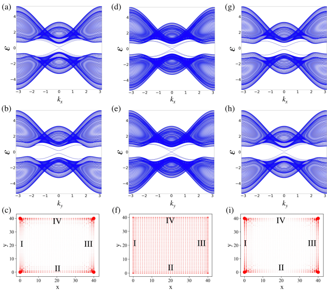
Figure 1: Band structure of a ribbon geometry along (a) $x$-direction and (b) $y$-direction with $s$-wave pairings and $\alpha=0$. 60 lattices is chosen along the direction with open boundary condition. (c) The normalized local density of states at $\varepsilon=0$ for the same sample with lattices $N\times N=41\times 41$ and open boundary condition. In (d)-(f) $\alpha=0.5$ and in (g)-(i) $\alpha=1.$ Other parameters are the same for all panels: $m_{0}=1$, $t=2$, $\lambda=1$, $\Delta_{s}=0.2$, $m_{x}=0.3$ and $m_{y}=0$.

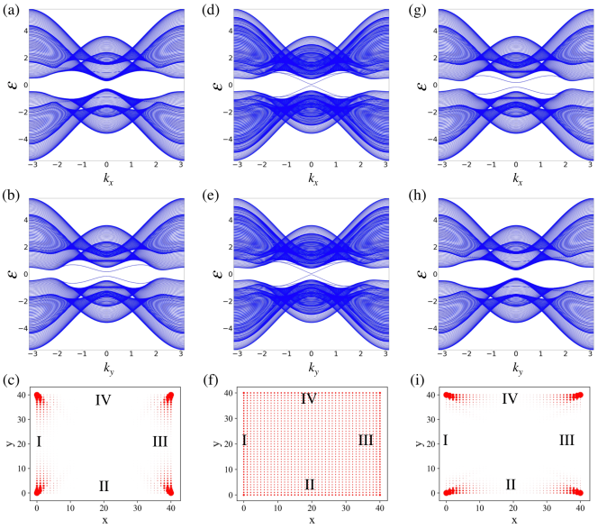
Figure 2: Band structure and normalized local density of states at $\varepsilon=0$ for $d$-wave pairings. $\alpha=0$ for left panels, $\alpha=0.5$ for middle panels, and $\alpha=1$ for right panels. Other parameters are the same as Fig. 1 except for $\Delta_{d}=0.2$ and $m_{x}=0.6$.

Majorana corner modes.— We first show the energy spectrum of 2D magnetic TI in proximity to a superconductor. The aim for the band calculation is to testify the gap opening by Dirac mass in Eqs. 6-7. We use a ribbon geometry with open boundary conditions along the $x$ direction or $y$ direction and generate the band structure of $\hat{H}_{\mathbf{i},\mathbf{j}}$ using exact diagonalization. The lattices of the ribbon width is fixed at $N=60$. To obtain the LDOSs, we use a sample with lattices $N\times N=41\times 41$ and open boundary condition.

Figure 1 plots band structure and local density of states in the $s$-wave pairing state. The degenerate energy bands split due to non-zero in-plane magnetic field. When $\alpha=0$, two orbitals experience the same exchange interaction, and we recover the known results of MCMs  [33] in Fig. 1(c). However, we find no MCMs for $\alpha=0.5$ with same band parameters as shown in Fig. 1(f). When $\alpha=1$, the MCMs reappear at four corners (see Fig. 1 (i)) though the two orbitals now have opposite exchange splittings. This indicates that the orbital difference $\alpha$ is a critical parameter which can induce the topological phase transition in SOTS. Then we calculate the same sample by replacing $s$-wave paring state by $d$-wave one as shown in Fig. 2. We observe the topological phase transition by $\alpha$ and for large $m_{x}$. It is necessary to point out that by measuring the local density of states alone can not identify the number of MCMs located at the four corners of the sample.

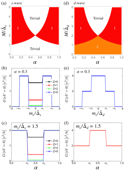
Figure 3: (a)(d) Phase diagram of superconductivity in the $\alpha$-$M/\tilde{\Delta}_{s\left(d\right)}$ plane. The white region is topologically trivial. The region 1 (red) indicates the phase with a single MCM at each corner. The region 2 (orange) indicates the phase with a pair of MCMs at each corner. (b)(c) are the zero bias conductance for $s$-wave pairing state while (e) and (f) for $d$-wave case.

Topological analysis.— Let us investigate the condition for MCMs based on effective Hamiltonian on edges. We choose two specific adjacent edges: I and IV. Making a unitary transformation

$$U=\frac{1}{\sqrt{2}}\left[\begin{array}[]{cccc}1&0&e^{-i\theta}&0\\ 0&1&0&-e^{i\theta}\\ 0&e^{-i\theta}&0&1\\ e^{i\theta}&0&-1&0\end{array}\right],$$ (15)

we find that the I edge can be described by the following Hamiltonian $\breve{H}_{\text{I}}=U\tilde{H}_{\text{I}}U^{{\dagger}}=h_{\text{I},1}\oplus h_{\text{I},2}$, with

$$h_{\text{I},1}=\left[\begin{array}[]{cc}i\lambda\partial_{y}&e^{-i\theta}\left[\alpha M\mp\tilde{\Delta}_{s\left(d\right)}\right]\\ e^{i\theta}\left[\alpha M\mp\tilde{\Delta}_{s\left(d\right)}\right]&-i\lambda\partial_{y}\end{array}\right],$$ (16)

$$h_{\text{I},2}=\left[\begin{array}[]{cc}-i\lambda\partial_{y}&e^{-i\theta}\left[\alpha M\pm\tilde{\Delta}_{s\left(d\right)}\right]\\ e^{i\theta}\left[\alpha M\pm\tilde{\Delta}_{s\left(d\right)}\right]&i\lambda\partial_{y}\end{array}\right].$$ (17)

and the IV edge is transformed into $\breve{H}_{\text{IV}}=U\tilde{H}_{\text{IV}}U^{{\dagger}}=h_{\text{IV},1}\oplus h_{\text{IV},2}$, with

$$h_{\text{IV},1} = \left[\begin{array}[]{cc}i\lambda\partial_{x}&e^{-i\theta}\Lambda_{1}\\ e^{i\theta}\Lambda_{1}&-i\lambda\partial_{x}\end{array}\right],$$ (20)

$$h_{\text{IV},2} = \left[\begin{array}[]{cc}-i\lambda\partial_{x}&e^{-i\theta}\Lambda_{2}\\ e^{i\theta}\Lambda_{2}&i\lambda\partial_{x}\end{array}\right],$$ (23)

$$\Lambda_{1} = \left(1-\alpha\right)M-\tilde{\Delta}_{s\left(d\right)},$$ (24)

$$\Lambda_{2} = \left(1-\alpha\right)M+\tilde{\Delta}_{s\left(d\right)}.$$ (25)

According to the Jackiw-Rebbi theory [42], the existence of MCMs for $s$-wave pair potential requires that

$$\left(\alpha M/\tilde{\Delta}_{s}-1\right)\left[\left(1-\alpha\right)M/\tilde{\Delta}_{s}-1\right]<0.$$ (26)

It is noted that angle $\theta$ does not plays a role in Eq. 26, thus the topological condition only depends on the magnitude of magnetization $M$ and effective pair potential $\tilde{\Delta}_{s}$. The phase diagram is shown in Fig. 3(a) where the shaded region indicates the SOTS. Such diagram agrees well with the numerical result in Fig. 1. It can be seen that under the condition $M>\tilde{\Delta}_{s}$, the system undergoes topological phase transition by increasing $\alpha$ from $0$ to $1$. Moreover, the system stays in the trivial states for an intermediate value of $\alpha=0.5$ regardless of $M$.

For $d$-wave pair potential, it can be verified that pairs of MCMs can be found under the condition $d_{1}<0$ and $d_{2}<0$ where $d_{1}$ and $d_{2}$ are given by

$$d_{1} = \left(\alpha M/\tilde{\Delta}_{d}+1\right)\left[\left(1-\alpha\right)M/\tilde{\Delta}_{d}-1\right],$$ (27)

$$d_{2} = \left(\alpha M/\tilde{\Delta}_{d}-1\right)\left[\left(1-\alpha\right)M/\tilde{\Delta}_{d}+1\right].$$ (28)

When $d_{1}$ and $d_{2}$ satisfy $d_{1}d_{2}<0$, a single MCM exists. For $d$-wave pairings, the pair potential undergoes a sign change for adjacent edges, which provides additional sign change of the mass term leading to pairs of MCMs. It is also interesting to note that the phase diagram of $d$-wave pairing (see Fig. 3(d)) resembles the phase diagram of $s$-wave case. However, pairs of MCMs form for $M<$ $\tilde{\Delta}_{d}$ regardless of $\alpha$ due to the unconventional $d$-wave pairing.

Experimental signatures.— To explore the experimental signatures of the MCMs, we propose to use a normal probe terminal, such as an STM tip, coupled to the corner of the SOTS. Specifically, the semi-infinite normal probe on the $x$-axis is placed at the corner between I and IV edges. We set the origin at the corner and the Hamiltonian $H_{N}$ of the probe is

$$H_{N}=\left[-\frac{\partial_{x}^{2}}{2\tilde{m}}-\mu_{N}+U\delta\left(x+0^{+}\right)\right]\hat{\tau}_{z},$$ (29)

where $\tilde{m}$, $\mu_{N}$ and $U$ are the effective mass, chemical potential and the barrier parameter between the probe and the 2D TI, respectively. For simplicity, we only consider $x$-axis magnetization. Using the similar method [43, 44, 45], one can obtain the boundary condition which connects the wave functions $\Psi_{N}$ of the normal probe, $\Psi_{\text{I}}$ and $\Psi_{\text{IV}}$ of the edge I and IV at the corner as follows

$$\Psi_{N} = \chi\left(\Psi_{\text{I}}+\Psi_{\text{IV}}\right),$$ (30)

$$\chi\left(\partial_{x}\Psi_{N}+Zk\Psi_{N}\right) = i\lambda\tilde{m}\hat{s}_{z}\hat{\tau}_{z}\left(\Psi_{\text{I}}-\Psi_{\text{IV}}\right).$$ (31)

The parameter $Z=2\tilde{m}U/k$ ($k$: the Fermi wave vector) describes the barrier strength, while the real and dimensionless number $\chi$ represents the different microscopic details between the probe and 2D TI, such as the hopping integrals in the underlying lattice model. The scattering wave function for the normal probe is solved as

$$\Psi_{N\sigma}={} \Phi_{\sigma}+b_{\uparrow\sigma}\hat{B}_{\uparrow}e^{-ikx}+b_{\downarrow\sigma}\hat{B}_{\downarrow}e^{-ikx}$$

$$+a_{\uparrow\sigma}\hat{A}_{\uparrow}e^{ikx}+a_{\downarrow\sigma}\hat{A}_{\downarrow}e^{ikx},$$ (32)

for an incident electron with spin $\sigma=\uparrow(\downarrow)$ and wave function $\Phi_{\uparrow}=(1,0,0,0)^{T}e^{iqx}$ [$\Phi_{\downarrow}=(0,1,0,0)^{T}e^{iqx}$]. Under the wide band approximation, the wave vector is $k=\sqrt{2m_{N}\mu_{N}}$ and the spinors are $\hat{B}_{\uparrow}=(1,0,0,0)^{T}$, $\hat{B}_{\downarrow}=(0,1,0,0)^{T}$, $\hat{A}_{\uparrow}=(0,0,1,0)^{T}$, and $\hat{A}_{\downarrow}=(0,0,0,1)^{T}$. The normal (Andreev) reflection amplitudes are $b_{\sigma^{\prime}\sigma}$ ($a_{\sigma^{\prime}\sigma}$) for an incoming electron of spin $\sigma$ scattered as an electron (hole) of spin $\sigma^{\prime}$. We focus on zero energy solution and thus the wave functions of edge I and IV are

$$\Psi_{\text{IV,}\sigma} = c_{1\sigma}\Phi_{1}\left(p_{1}\right)e^{-\left|p_{1}\right|x}+c_{2\sigma}\Phi_{2}\left(p_{2}\right)e^{-\left|p_{2}\right|x},$$ (33)

$$\Psi_{\text{I,}\sigma} = d_{1\sigma}\Phi_{3}\left(p_{3}\right)e^{\left|p_{3}\right|y}+d_{2\sigma}\Phi_{4}\left(p_{4}\right)e^{\left|p_{4}\right|y}.$$ (34)

with $\Phi_{1\left(2\right)}\left(\kappa\right)=(\pm\nu,\mp 1,\nu,1)^{T}$, $\Phi_{3\left(4\right)}\left(\kappa\right)=(\nu,1,\mp\nu,\pm 1)^{T}$ and $\nu=i\kappa/\left|\kappa\right|$. For $s$-wave pair potential, we have $\lambda p_{1\left(2\right)}=m_{x}-\alpha m_{x}\mp\tilde{\Delta}_{s}$, $\lambda p_{3\left(4\right)}=\alpha m_{x}\pm\tilde{\Delta}_{s}$ and they are $\lambda p_{1\left(2\right)}=m_{x}-\alpha m_{x}\mp\tilde{\Delta}_{d}$, $\lambda p_{3\left(4\right)}=\alpha m_{x}\mp\tilde{\Delta}_{d}$ for $d$-wave case. The differential conductance $G$ at zero temperature is calculated using the formula [46]

$$G=\frac{e^{2}}{h}\sum\nolimits_{\sigma\sigma^{\prime}}\left[\delta_{\sigma\sigma^{\prime}}+\left|a_{\sigma\sigma^{\prime}}\right|^{2}-\left|b_{\sigma\sigma^{\prime}}\right|^{2}\right].$$ (35)

Here, $a_{\sigma\sigma^{\prime}}$ and $b_{\sigma\sigma^{\prime}}$ are reflection amplitudes at zero bias. For the numerical calculations we choose $k_{N}/\tilde{m}\approx 1.57\times 10^{6}$ m/s, $\mu_{N}\approx 7.0$ eV corresponding to copper, $\left|\lambda\right|\approx 5.5\times 10^{5}$ m/s and $\chi=1$. We note that the feature of zero-bias conductance is not material dependent.

First, we display the result of zero bias conductance for $s$-wave pairing state. For a fixed $\alpha$, the phase boundary clearly appears in the conductance dependence on the magnetization $m_{x}$ in Fig. 3(b). It can be seen that the zero-bias conductance clearly showcases the celebrated Majorana zero bias peak with quantized height $2e^{2}/h$ [47, 48, 49, 50, 51] for $m_{1}<\left|m_{x}\right|<m_{2}$. And as the quantized conductance appears, it remains a plateau by altering the barrier $Z$. For $\left|m_{x}\right|<m_{1}$, the system enters into non-topological phase and the conductance can be greatly affected by $Z$. Moreover, the conductance becomes almost $0$ for $\left|m_{x}\right|>m_{2}$ as the system is no longer topological. This suppressed conductance can be explained by a large opening gap due to magnetization where all waves on edges become evanescent. In Fig. 3(c) , we show how a quantum plateau of the zero-biased conductance can be tuned out for a given $m_{x}$, by altering band difference $\alpha$. The conductance becomes sensitive to the barrier $Z$ for $\alpha_{1}<\alpha<\alpha_{2}$ which reflects no MCM. The result of conductance agrees well with the phase diagram as shown in Fig. 3(a) and provides a support for experimental detection of MCMs by tunneling spectroscopy.

We now turn to the $d$-wave case. At zero magnetization, it has been known that there are pairs of MCMs. Our conductance result shows a $4e^{2}/h$ conductance peak as the presence of pairs of MCMs even in a weak exchange field $\left|m_{x}\right|<m_{1}$ in Fig. 3(e). We do note specify the used value of $Z$ since this conductance is immune to its variation. For $m_{1}<\left|m_{x}\right|<m_{2}$, we obtain a $2e^{2}/h$ conductance plateau similar to the $s$-wave case, indicating a single MCM at each corner. And as $\left|m_{x}\right|$ is greater than $m_{2}$, the system become topological trivial and gives rises to suppressed conductance due to the magnetic gap. It shows that the conductance quantization is robust in each topological phase as $\alpha$ changes for a given $m_{x}$, as shown in Fig. 3(f). These results are consistent with the phase diagram in Fig. 3(d). We can see that the tunneling spectroscopy is a useful way of not only providing the information of the presence of MCMs, but also the number of them.

Conclusions.— We have studied the orbital-dependent exchange field effect on the formation of second order topological superconductors based on two-dimensional topological insulators. We have considered both $s$-wave and $d$-wave pairing states. The Majorana corner modes are shown to be dependent on the orbital difference. For experimental realizations, we expect 2D topological insulator materials such as HgTe quantum wells. When proximate to superconductors, a proximity-induced superconducting gap can be induced [52]. And when doping with Mn, the magnetization of HgTe shows orbital difference under an in-plane magnetic field [53]. And an in-plane magnetic field has been successfully coulped to HgTe quantum wells in recent experiments [54]. We finally propose an experiment to demonstrate that the quantized zero-biased conductance indeed arises due to the Majorana corner modes.

Acknowledgments.— We acknowledge support from the National Natural Science Foundation of China (project 11904257) and the Natural Science Foundation of Tianjin (project 20JCQNJC01310).

References

- Hasan and Kane [2010] M. Z. Hasan and C. L. Kane, Colloquium: Topological insulators, Rev. Mod. Phys. 82, 3045 (2010).
- Qi and Zhang [2011] X.-L. Qi and S.-C. Zhang, Topological insulators and superconductors, Rev. Mod. Phys. 83, 1057 (2011).
- Fu et al. [2007] L. Fu, C. L. Kane, and E. J. Mele, Topological insulators in three dimensions, Phys. Rev. Lett. 98, 106803 (2007).
- Fu and Kane [2007] L. Fu and C. L. Kane, Topological insulators with inversion symmetry, Phys. Rev. B 76, 045302 (2007).
- Kou et al. [2015] X. Kou, Y. Fan, M. Lang, P. Upadhyaya, and K. L. Wang, Magnetic topological insulators and quantum anomalous hall effect, Solid State Communications 215-216, 34 (2015).
- Chang and Li [2016] C.-Z. Chang and M. Li, Quantum anomalous hall effect in time-reversal-symmetry breaking topological insulators, Journal of Physics: Condensed Matter 28, 123002 (2016).
- He et al. [2018] K. He, Y. Wang, and Q.-K. Xue, Topological materials: Quantum anomalous hall system, Annual Review of Condensed Matter Physics 9, 329 (2018).
- Tokura et al. [2019] Y. Tokura, K. Yasuda, and A. Tsukazaki, Magnetic topological insulators, Nature Reviews Physics 1, 126 (2019).
- Alicea [2012] J. Alicea, New directions in the pursuit of majorana fermions in solid state systems, Reports on Progress in Physics 75, 076501 (2012).
- Beenakker [2013] C. Beenakker, Search for majorana fermions in superconductors, Annual Review of Condensed Matter Physics 4, 113 (2013).
- Sato and Fujimoto [2016] M. Sato and S. Fujimoto, Majorana fermions and topology in superconductors, Journal of the Physical Society of Japan 85, 072001 (2016).
- Kitaev [2001] A. Kitaev, Unpaired majorana fermions in quantum wires, Physics-Uspekhi 44, 131 (2001).
- Kitaev [2003] A. Kitaev, Fault-tolerant quantum computation by anyons, Annals of Physics 303, 2 (2003).
- Nayak et al. [2008] C. Nayak, S. H. Simon, A. Stern, M. Freedman, and S. Das Sarma, Non-abelian anyons and topological quantum computation, Rev. Mod. Phys. 80, 1083 (2008).
- Langbehn et al. [2017] J. Langbehn, Y. Peng, L. Trifunovic, F. von Oppen, and P. W. Brouwer, Reflection-symmetric second-order topological insulators and superconductors, Phys. Rev. Lett. 119, 246401 (2017).
- Zhu [2018] X. Zhu, Tunable majorana corner states in a two-dimensional second-order topological superconductor induced by magnetic fields, Phys. Rev. B 97, 205134 (2018).
- Khalaf [2018] E. Khalaf, Higher-order topological insulators and superconductors protected by inversion symmetry, Phys. Rev. B 97, 205136 (2018).
- Wang et al. [2018a] Y. Wang, M. Lin, and T. L. Hughes, Weak-pairing higher order topological superconductors, Phys. Rev. B 98, 165144 (2018a).
- Yan et al. [2018] Z. Yan, F. Song, and Z. Wang, Majorana corner modes in a high-temperature platform, Phys. Rev. Lett. 121, 096803 (2018).
- Wang et al. [2018b] Q. Wang, C.-C. Liu, Y.-M. Lu, and F. Zhang, High-temperature majorana corner states, Phys. Rev. Lett. 121, 186801 (2018b).
- Liu et al. [2018] T. Liu, J. J. He, and F. Nori, Majorana corner states in a two-dimensional magnetic topological insulator on a high-temperature superconductor, Phys. Rev. B 98, 245413 (2018).
- Pan et al. [2019] X.-H. Pan, K.-J. Yang, L. Chen, G. Xu, C.-X. Liu, and X. Liu, Lattice-symmetry-assisted second-order topological superconductors and majorana patterns, Phys. Rev. Lett. 123, 156801 (2019).
- Hsu et al. [2018] C.-H. Hsu, P. Stano, J. Klinovaja, and D. Loss, Majorana kramers pairs in higher-order topological insulators, Phys. Rev. Lett. 121, 196801 (2018).
- Volpez et al. [2019] Y. Volpez, D. Loss, and J. Klinovaja, Second-order topological superconductivity in -junction rashba layers, Phys. Rev. Lett. 122, 126402 (2019).
- Zhu [2019] X. Zhu, Second-order topological superconductors with mixed pairing, Phys. Rev. Lett. 122, 236401 (2019).
- Franca et al. [2019] S. Franca, D. V. Efremov, and I. C. Fulga, Phase-tunable second-order topological superconductor, Phys. Rev. B 100, 075415 (2019).
- Ghorashi et al. [2019] S. A. A. Ghorashi, X. Hu, T. L. Hughes, and E. Rossi, Second-order dirac superconductors and magnetic field induced majorana hinge modes, Phys. Rev. B 100, 020509 (2019).
- Zeng et al. [2019] C. Zeng, T. D. Stanescu, C. Zhang, V. W. Scarola, and S. Tewari, Majorana corner modes with solitons in an attractive hubbard-hofstadter model of cold atom optical lattices, Phys. Rev. Lett. 123, 060402 (2019).
- Laubscher et al. [2019] K. Laubscher, D. Loss, and J. Klinovaja, Fractional topological superconductivity and parafermion corner states, Phys. Rev. Research 1, 032017 (2019).
- Roy [2019] B. Roy, Antiunitary symmetry protected higher-order topological phases, Phys. Rev. Research 1, 032048 (2019).
- Zhang and Trauzettel [2020] S.-B. Zhang and B. Trauzettel, Detection of second-order topological superconductors by josephson junctions, Phys. Rev. Research 2, 012018 (2020).
- Roy [2020] B. Roy, Higher-order topological superconductors in -, -odd quadrupolar dirac materials, Phys. Rev. B 101, 220506 (2020).
- Wu et al. [2020] Y.-J. Wu, J. Hou, Y.-M. Li, X.-W. Luo, X. Shi, and C. Zhang, In-plane zeeman-field-induced majorana corner and hinge modes in an -wave superconductor heterostructure, Phys. Rev. Lett. 124, 227001 (2020).
- Kheirkhah et al. [2020] M. Kheirkhah, Z. Yan, Y. Nagai, and F. Marsiglio, First- and second-order topological superconductivity and temperature-driven topological phase transitions in the extended hubbard model with spin-orbit coupling, Phys. Rev. Lett. 125, 017001 (2020).
- Zhang et al. [2020a] S.-B. Zhang, A. Calzona, and B. Trauzettel, All-electrically tunable networks of majorana bound states, Phys. Rev. B 102, 100503 (2020a).
- Zhang et al. [2020b] S.-B. Zhang, W. B. Rui, A. Calzona, S.-J. Choi, A. P. Schnyder, and B. Trauzettel, Topological and holonomic quantum computation based on second-order topological superconductors, Phys. Rev. Research 2, 043025 (2020b).
- Li and Zhou [2021] Y.-X. Li and T. Zhou, Rotational symmetry breaking and partial majorana corner states in a heterostructure based on high- superconductors, Phys. Rev. B 103, 024517 (2021).
- Kheirkhah et al. [2021] M. Kheirkhah, Z. Yan, and F. Marsiglio, Vortex-line topology in iron-based superconductors with and without second-order topology, Phys. Rev. B 103, L140502 (2021).
- Luo et al. [2021] X.-J. Luo, X.-H. Pan, and X. Liu, Higher-order topological superconductors based on weak topological insulators, Phys. Rev. B 104, 104510 (2021).
- Ren et al. [2020] Y. Ren, Z. Qiao, and Q. Niu, Engineering corner states from two-dimensional topological insulators, Phys. Rev. Lett. 124, 166804 (2020).
- Shen [2017] S.-Q. Shen, Topological insulators: Dirac equation in condensed matter, 2nd ed., (Springer, Singapore) (2017).
- Jackiw and Rebbi [1976] R. Jackiw and C. Rebbi, Solitons with fermion number ½, Phys. Rev. D 13, 3398 (1976).
- Modak et al. [2012] S. Modak, K. Sengupta, and D. Sen, Spin injection into a metal from a topological insulator, Phys. Rev. B 86, 205114 (2012).
- Soori et al. [2013] A. Soori, O. Deb, K. Sengupta, and D. Sen, Transport across a junction of topological insulators and a superconductor, Phys. Rev. B 87, 245435 (2013).
- Soori [2020] A. Soori, Scattering in quantum wires and junctions of quantum wires with edge states of quantum spin hall insulators (2020), arXiv:2005.11557 [cond-mat.mes-hall] .
- Blonder et al. [1982] G. E. Blonder, M. Tinkham, and T. M. Klapwijk, Transition from metallic to tunneling regimes in superconducting microconstrictions: Excess current, charge imbalance, and supercurrent conversion, Phys. Rev. B 25, 4515 (1982).
- Sengupta et al. [2001] K. Sengupta, I. Žutić, H.-J. Kwon, V. M. Yakovenko, and S. Das Sarma, Midgap edge states and pairing symmetry of quasi-one-dimensional organic superconductors, Phys. Rev. B 63, 144531 (2001).
- Bolech and Demler [2007] C. J. Bolech and E. Demler, Observing majorana bound states in -wave superconductors using noise measurements in tunneling experiments, Phys. Rev. Lett. 98, 237002 (2007).
- Akhmerov et al. [2009] A. R. Akhmerov, J. Nilsson, and C. W. J. Beenakker, Electrically detected interferometry of majorana fermions in a topological insulator, Phys. Rev. Lett. 102, 216404 (2009).
- Tanaka et al. [2009] Y. Tanaka, T. Yokoyama, and N. Nagaosa, Manipulation of the majorana fermion, andreev reflection, and josephson current on topological insulators, Phys. Rev. Lett. 103, 107002 (2009).
- Law et al. [2009] K. T. Law, P. A. Lee, and T. K. Ng, Majorana fermion induced resonant andreev reflection, Phys. Rev. Lett. 103, 237001 (2009).
- Bocquillon et al. [2017] E. Bocquillon, R. S. Deacon, J. Wiedenmann, P. Leubner, T. M. Klapwijk, C. Brüne, K. Ishibashi, H. Buhmann, and L. W. Molenkamp, Gapless Andreev bound states in the quantum spin Hall insulator HgTe, Nature Nanotechnology 12, 137 (2017).
- Liu et al. [2013] X. Liu, H.-C. Hsu, and C.-X. Liu, In-plane magnetization-induced quantum anomalous hall effect, Phys. Rev. Lett. 111, 086802 (2013).
- Ren et al. [2019] H. Ren, F. Pientka, S. Hart, A. T. Pierce, M. Kosowsky, L. Lunczer, R. Schlereth, B. Scharf, E. M. Hankiewicz, L. W. Molenkamp, B. I. Halperin, and A. Yacoby, Topological superconductivity in a phase-controlled josephson junction, Nature 569, 93 (2019).