Quasi-normal modes of dyonic black holes and magneto-hydrodynamics

Abstract

We revisit the magneto-hydrodynamics in (2+1) dimensions and confirm that it is consistent with the quasi-normal modes of the (3+1) dimensional dyonic black holes in the most general set-up with finite density, magnetic field and wave vector. We investigate all possible modes (sound, shear, diffusion, cyclotron etc.) and their interplay. For the magneto-hydrodynamics we perform a complete and detailed analysis correcting some prefactors in the literature, which is important for the comparison with quasi-normal modes. For the quasi-normal mode computations in holography we identify the independent fluctuation variables of the dyonic black holes, which is nontrivial at finite density and magnetic field. As an application of the quasi-normal modes of the dyonic black holes we investigate a transport property, the diffusion constant. We find that the diffusion constant at finite density and magnetic field saturates the lower bound at low temperature. We show that this bound can be understood from the pole-skipping point.

1 Introduction

Holography (gauge/gravity duality) has provided useful methods to study properties of strongly coupled systems Hartnoll:2016apf ; Zaanen:2015oix ; Ammon:2015wua ; Baggioli:2019rrs . In particular, the holographic descriptions of the strongly correlated (2+1) dimensional collective dynamics have been implemented to shed light on long-standing condensed matter problems such as the quantum phase transition Hartnoll:2007ih , superfluidity Basu:2008st ; Herzog:2008he , high-temperature superconductivity Hartnoll:2008vx ; Hartnoll:2008kx .

One of the milestones for the strongly coupled (2+1) dimensional field theories in holography is that the quasi-normal modes of the (3+1) dimensional AdS black holes are consistent with the predictions of (2+1) dimensional hydrodynamics, for instance, the holographic model with the explicitly (or spontaneously) broken translational symmetry Davison:2014lua ; Amoretti:2017frz ; Andrade:2017cnc ; Amoretti:2018tzw ; Ammon:2019wci ; Amoretti:2019cef ; Amoretti:2019kuf ; Baggioli:2021xuv ; Jeong:2021zhz and the superfluid where the U(1) symmetry is broken spontaneously Amado:2009ts ; Herzog:2009md ; Yarom:2009uq ; Herzog:2011ec ; Amado:2013xya ; Amado:2013aea ; Esposito:2016ria ; Arean:2021tks or pseudo-spontaneously Ammon:2021slb .

Comparing the quasi-normal modes with hydrodynamic predictions will be an important and interesting research direction because it may not only provide more supporting (indirect) evidence of holographic duality, but also gives us novel analysis for the transport properties of strongly correlated systems. Note that hydrodynamics can tell which transport coefficients appear in the theory and holography reveals the details of the transport properties of such coefficients.

In this paper, we study the (3+1) dimensional AdS black hole in the presence of external magnetic fields at finite density, dyonic black holes (Einstein-Maxwell model), which is dual to the (2+1) dimensional quantum field theory in external magnetic fields. In particular, we aim to compute the quasi-normal modes of dyonic black holes and compare them with the viscous magneto-hydrodynamics proposed by Hartnoll-Kovtun-Müller-Sachdev (HKMS) Hartnoll:2007ih . Thus, this paper is along the line of the developments of “the comparison between the quasi-normal modes in (3+1) dimensions and the hydrodynamics in (2+1) dimensions” in holography Davison:2014lua ; Amoretti:2017frz ; Andrade:2017cnc ; Amoretti:2018tzw ; Ammon:2019wci ; Amoretti:2019cef ; Amoretti:2019kuf ; Baggioli:2021xuv ; Jeong:2021zhz ; Amado:2009ts ; Herzog:2009md ; Yarom:2009uq ; Herzog:2011ec ; Amado:2013xya ; Amado:2013aea ; Esposito:2016ria ; Arean:2021tks ; Ammon:2021slb .

The dyonic black holes in (3+1) dimensions is one of well-studied black hole models in holography from the thermodynamic properties Hartnoll:2007ih ; Hartnoll:2007ip ; Hartnoll:2007ai ; Herzog:2007ij ; Denef:2009yy to the transport properties OBannon:2007in ; Buchbinder:2008dc ; Buchbinder:2009aa ; Buchbinder:2009mk ; Bergman:2012na ; Gubankova:2013lca ; Dutta:2013dca ; Kim:2015wba ; Amoretti:2015gna ; Blake:2015ina ; Lucas:2015pxa ; Zhou:2015dha ; Davison:2015bea ; Blake:2015hxa ; Donos:2015bxe ; Seo:2015pug ; Ahn:2015shg ; Amoretti:2016cad ; Kim:2016hzi ; Ge:2016sel ; Khimphun:2017mqb ; Blake:2017qgd ; Cremonini:2017qwq ; Seo:2017yux ; Chen:2017gsl ; Blauvelt:2017koq ; Angelinos:2018qlc ; Pal:2019bfw ; Kim:2019lxb ; Hoyos:2019pyz ; Song:2019rnf ; Amoretti:2019buu ; Baggioli:2020edn ; An:2020tkn ; Kim:2020ozm22 ; Amoretti:2020mkp ; Amoretti:2021lll ; Amoretti:2021fch ; Jokela:2021uws ; Priyadarshinee:2021rch such as the Hall conductivity, Nernst Effect, diverse magneto-transport and magnetic phase transition. However, surprisingly enough, a complete study of the quasi-normal mode excitations in dyonic black holes has been still lacking up to date.

In Jeong:2021zhz , quasi-normal modes of magnetically charged black holes (i.e., zero density) have been compared with the hydrodynamic theory only for the sound channel. As we will describe in the main context, at zero density, there will be two decoupled channels: the sound channel and the shear channel. In this paper, we fill the gap for the complete study of quasi-normal modes of (3+1) dimensional dyonic black holes. In other words, we compute the quasi-normal modes from all the channels (sound channel, shear channel) at zero density as well as the case at finite density in which the sound channel is coupled with the shear channel and compare all quasi-normal modes with the HKMS magneto-hydrodynamics Hartnoll:2007ih .

In addition to checking quasi-normal modes of dyonic black holes with the HKMS magneto-hydrodynamics, we also study the transport property that appeared at finite wave vector: the diffusion constant. In particular, we focus on the bound of the diffusion constant of dyonic black holes and study its relation with the pole-skipping argument Blake:2018leo ; Jeong:2021zhz .

This paper is organized as follows. In section 2, we revisit the HKMS magneto-hydrodynamics in (2+1) dimensions in details. In section 3, we introduce (3+1) dimensional dyonic black holes as well as the method for quasi-normal modes computation: the determinant method. Then, implementing the determinant method, we compute the quasi-normal modes of dyonic black holes and compare them with the hydrodynamic predictions given in section 2. Also we study the bound of the diffusion constant and the pole-skipping. Section 4 is devoted to conclusions.

2 Magneto-hydrodynamics revisited

In this section, we revisit the viscous magneto-hydrodynamics in (2+1) dimensions in the presence of the density ($\rho$) and the magnetic field ($H$), which is proposed by Hartnoll-Kovtun-Müller-Sachdev (HKMS) Hartnoll:2007ih .

It will be instructive to note that the main interest in Hartnoll:2007ih is the transport properties at zero wave vector such as conductivities OBannon:2007in ; Buchbinder:2008dc ; Buchbinder:2009aa ; Buchbinder:2009mk ; Bergman:2012na ; Kim:2015wba ; Amoretti:2015gna ; Lucas:2015pxa ; Zhou:2015dha ; Davison:2015bea ; Blake:2015hxa ; Donos:2015bxe ; Seo:2015pug ; Ahn:2015shg ; Amoretti:2016cad ; Kim:2016hzi ; Ge:2016sel ; Khimphun:2017mqb ; Blake:2017qgd ; Cremonini:2017qwq ; Seo:2017yux ; Chen:2017gsl ; Blauvelt:2017koq ; Angelinos:2018qlc ; Pal:2019bfw ; Kim:2019lxb ; Hoyos:2019pyz ; Song:2019rnf ; Amoretti:2019buu ; Baggioli:2020edn ; An:2020tkn ; Kim:2020ozm22 ; Amoretti:2020mkp ; Amoretti:2021lll ; Amoretti:2021fch ; Priyadarshinee:2021rch . In this paper, we study the properties of HKMS magneto-hydrodynamics at finite wave vector. Thus we aim to study the complete analysis of the HKMS magneto-hydrodynamics. In particular, we focus on the dispersion relations as well as the transport properties that appeared at finite wave vector such as the diffusion constant. Note that, in the main context below, we will revise two things about the dispersion relations given in the appendix of Hartnoll:2007ih : one is a sign typo and the other is the prefactor in the gapless hydrodynamic mode, which is important to be consistent with quasi-normal modes from holography.

2.1 Equations of motion

The equations of motion for hydrodynamics are the conservation laws:

$$\begin{split}\partial^{\nu}T_{\mu\nu}=F_{\mu\nu}J^{\nu}\,,\qquad\partial_{\mu}J^{\mu}=0,\end{split}$$ (1)

where $F_{\mu\nu}$ is the field strength of the electromagnetic field, $T_{\mu\nu}$ is the stress tenser, and $J^{\mu}$ is the current. In the case under consideration, we take $F_{\mu\nu}$ to be magnetic as

$$\begin{split}F_{tx}=0\,,\quad F_{ty}=0\,,\quad F_{ij}=\epsilon_{ij}H\,,\end{split}$$ (2)

where $i,j=(x,y)$. One can find the stress tensor $T_{\mu\nu}$ at first order in derivatives as

$$\begin{split}T^{\mu\nu}\,=\,\epsilon u^{\mu}u^{\nu}+P\Delta^{\mu\nu}+\Pi^{\mu\nu}\,,\end{split}$$ (3)

where $\epsilon$ is the energy density, $P$ is the pressure, and $\Delta^{\mu\nu}=\eta^{\mu\nu}+u^{\mu}u^{\nu}$ with the fluid velocity $u^{\mu}$. $\Pi^{\mu\nu}$ is the dissipative term given by

$$\begin{split}\Pi^{\mu\nu}\,=\,-\eta\left[\Delta^{\mu\alpha}\Delta^{\nu\beta}(\partial_{\alpha}u_{\beta}+\partial_{\beta}u_{\alpha})-\Delta^{\mu\nu}\partial_{\gamma}u^{\gamma}\right]\,,\end{split}$$ (4)

where $\eta$ is the shear viscosity. Note that $\Pi^{\mu\nu}$ is vanishing at local equilibrium by definition.

Similarly, the current $J^{\mu}$ can also be expressed at first order as

$$\begin{split}J^{\mu}=\rho u^{\mu}+\nu^{\mu}\,,\end{split}$$ (5)

where $\rho$ is the charge density and $\nu^{\mu}$ is the dissipative part given by

$$\begin{split}\nu^{\mu}=\sigma\Delta^{\mu\nu}\left(-\partial_{\nu}\mu+F_{\nu\alpha}u^{\alpha}+\frac{\mu}{T}\partial_{\nu}T\right)\,,\end{split}$$ (6)

where $\sigma$ is the conductivity, $\mu$ is the chemical potential, and $T$ is the temperature.

Choosing four independent variables $(\delta u_{i\,=\,x,y},\,\delta T,\,\delta\mu)$, we study the fluctuations around the equilibrium in which

$$\begin{split}u^{\mu}=(1,0,0)\,,\qquad T=\text{constant}\,,\qquad\mu=\text{constant}\,.\end{split}$$ (7)

Based on (7), one can find that the relevant fluctuations for (3) and (5) are

$$\begin{split}\delta T^{tt}&=\left(\frac{\partial\epsilon}{\partial\mu}\right)_{T}\delta\mu+\left(\frac{\partial\epsilon}{\partial T}\right)_{\mu}\delta T\,,\qquad\qquad\qquad\qquad\qquad\delta T^{ti}=\left(\epsilon+P\right)\delta u_{i}\,,\\ \delta T^{ii}&=\left(\frac{\partial P}{\partial\mu}\right)_{T}\delta\mu+\left(\frac{\partial P}{\partial T}\right)_{\mu}\delta T-\eta(2\partial_{i}\delta u_{i}-\partial_{\gamma}\delta u_{\gamma})\,,\,\,\,\,\delta T^{ij}=-\eta(\partial_{j}\delta u_{i}+\partial_{i}\delta u_{j})\,,\\ \delta J^{t}&=\left(\frac{\partial\rho}{\partial\mu}\right)_{T}\delta\mu+\left(\frac{\partial\rho}{\partial T}\right)_{\mu}\delta T\,,\\ \delta J^{i}&=\rho\delta u_{i}+\sigma\left(-\partial_{i}\delta\mu+\frac{\mu}{T}\partial_{i}\delta T+H\varepsilon_{ij}\delta u_{j}\right)\,,\end{split}$$ (8)

where $\varepsilon_{ij}$ is the Levi-Civita symbol. Plugging (8) into the equations of motion (1) and also performing a Fourier transformation with the plane wave form $e^{-i\omega t+ikx}$, we obtain the four coupled equations:

$$\begin{split}0&=\omega\left[{\left(\frac{\partial{\epsilon}}{\partial{\mu}}\right)_{T}}\delta\mu+{\left(\frac{\partial{\epsilon}}{\partial{T}}\right)_{\mu}}\delta T\right]-k(\epsilon+P)\delta u_{x}\,,\\ 0&=\omega(\epsilon+P)\delta u_{x}-k\left[{\left(\frac{\partial{P}}{\partial{\mu}}\right)_{T}}\delta\mu+{\left(\frac{\partial{P}}{\partial{T}}\right)_{\mu}}\delta T\right]+ik^{2}\eta\,\delta u_{x}+i\sigma H^{2}\delta u_{x}-iH\rho\delta u_{y}\,,\\ 0&=\omega(\epsilon+P)\delta u_{y}+kH\sigma\left(\delta\mu-\frac{\mu}{T}\delta T\right)+iH\rho\delta u_{x}+i\sigma H^{2}\delta u_{y}+ik^{2}\eta\delta u_{y}\,,\\ 0&=\omega\left[{\left(\frac{\partial{\rho}}{\partial{\mu}}\right)_{T}}\delta\mu+{\left(\frac{\partial{\rho}}{\partial{T}}\right)_{\mu}}\delta T\right]-k\rho\delta u_{x}-k\sigma H\delta u_{y}+ik^{2}\sigma\left(\delta\mu-\frac{\mu}{T}\delta T\right)\,,\end{split}$$ (9)

which are consistent with equations in Hartnoll:2007ih where the thermodynamic relation $\epsilon+P=sT+\mu\rho$ holds. The equations of motion (9) can also be expressed as the matrix form, $\mathcal{M}\cdot\mathcal{V}=0$, with

$$\mathcal{M}:=\begin{pmatrix}-k(\epsilon+P)&\omega{\left(\frac{\partial{\epsilon}}{\partial{T}}\right)_{\mu}}&0&\omega{\left(\frac{\partial{\epsilon}}{\partial{\mu}}\right)_{T}}\\ \omega(\epsilon+P)+ik^{2}\eta+i\sigma H^{2}&-k{\left(\frac{\partial{P}}{\partial{T}}\right)_{\mu}}&-iH\rho&-k{\left(\frac{\partial{P}}{\partial{\mu}}\right)_{T}}\\ iH\rho&-\frac{kH\sigma\mu}{T}&\omega(\epsilon+P)+ik^{2}\eta+i\sigma H^{2}&kH\sigma\\ -k\rho&\omega{\left(\frac{\partial{\rho}}{\partial{T}}\right)_{\mu}}-\frac{ik^{2}\sigma\mu}{T}&-k\sigma H&\omega{\left(\frac{\partial{\rho}}{\partial{\mu}}\right)_{T}}+ik^{2}\sigma\end{pmatrix}$$ (10)

and the vector $\mathcal{V}:=(\delta u_{x},\,\delta T,\,\delta u_{y},\,\delta\mu)$. Then one can obtain the dispersion relations, $\omega=\omega(k)$, by the determinant of (10):

$$\begin{split}0\,=\,\text{det}\,\mathcal{M}\,:=\,\mathcal{M}_{1}+\mathcal{M}_{2}+\mathcal{M}_{3}\,,\end{split}$$ (11)

where

$$\begin{split}\mathcal{M}_{1}&=\omega\rho H^{2}\left[ik^{2}\sigma(\epsilon+P)\left(\mu{\left(\frac{\partial{\rho}}{\partial{\mu}}\right)_{T}}+T{\left(\frac{\partial{\rho}}{\partial{T}}\right)_{\mu}}\right)+\omega\rho T\left({\left(\frac{\partial{\epsilon}}{\partial{T}}\right)_{\mu}}{\left(\frac{\partial{\rho}}{\partial{\mu}}\right)_{T}}-{\left(\frac{\partial{\epsilon}}{\partial{\mu}}\right)_{T}}{\left(\frac{\partial{\rho}}{\partial{T}}\right)_{\mu}}\right)\right]\,,\\ \mathcal{M}_{2}&=ik^{2}T\sigma X(Z-iH^{2}\sigma)+\omega TZ\left(X{\left(\frac{\partial{\rho}}{\partial{\mu}}\right)_{T}}-Y{\left(\frac{\partial{\rho}}{\partial{T}}\right)_{\mu}}\right)+i\frac{Z}{H^{2}\sigma}\mathcal{M}_{3}\,,\\ \mathcal{M}_{3}&=k^{2}H^{2}\sigma\left[\mu\sigma Y-i\omega\rho T\left({\left(\frac{\partial{\epsilon}}{\partial{T}}\right)_{\mu}}{\left(\frac{\partial{P}}{\partial{\mu}}\right)_{T}}-{\left(\frac{\partial{\epsilon}}{\partial{\mu}}\right)_{T}}{\left(\frac{\partial{P}}{\partial{T}}\right)_{\mu}}\right)\right]\,,\end{split}$$ (12)

with

$$\begin{split}X&=k^{2}\left(\epsilon+P\right){\left(\frac{\partial{P}}{\partial{T}}\right)_{\mu}}-\omega\,Z\,{\left(\frac{\partial{\epsilon}}{\partial{T}}\right)_{\mu}}\,,\qquad Y=k^{2}\left(\epsilon+P\right){\left(\frac{\partial{P}}{\partial{\mu}}\right)_{T}}-\omega\,Z\,{\left(\frac{\partial{\epsilon}}{\partial{\mu}}\right)_{T}}\,,\\ Z&=\omega\left(\epsilon+P\right)+ik^{2}\eta+i\sigma H^{2}\,.\end{split}$$ (13)

In the following sections, we study the dispersion relations by (11)-(13) at zero density in Section 2.2 and at finite density in Section 2.3, respectively.

Note that the highest order of $\omega$ in (12) is $\mathcal{O}\left(\omega^{4}\right)$ from $\mathcal{M}_{2}$ so that one can solve (11) to obtain $\omega(k)$ explicitly. However, the analytic expression of $\omega(k)$ is not so illuminating and complicated so we do not show it here. Instead, we will display its plots when we compare with quasi-normal modes from holography in the next section: see solid lines in Fig. 1 and Fig. 2. Furthermore, for the analysis of hydrodynamic modes of $\omega(k)$, we will show the analytic expression of the dispersion relation at the small $k$ regime in the following subsections.

2.2 Zero density

Let us first consider the hydrodynamics with no density ($\rho=0$). Moreover, motivated by $M2$-brane magneto-hydrodynamics Buchbinder:2008dc , we may set

$$\begin{split}{\left(\frac{\partial{\rho}}{\partial{T}}\right)_{\mu}}={\left(\frac{\partial{\epsilon}}{\partial{\mu}}\right)_{T}}={\left(\frac{\partial{P}}{\partial{\mu}}\right)_{T}}=0\,,\end{split}$$ (14)

which will be verified by holography in the next section.

For the case of zero density with (14), one can check that $\mathcal{M}_{1}=\mathcal{M}_{3}=0$ in (12) so that (11) becomes

$$\begin{split}\quad 0\,=\,\mathcal{M}_{2}=X\left[Z\left(ik^{2}\sigma+\omega{\left(\frac{\partial{\rho}}{\partial{\mu}}\right)_{T}}\right)+k^{2}H^{2}\sigma^{2}\right]\,,\end{split}$$ (15)

where $X$ and $Z$ are given in (13). Note that $\mathcal{M}_{2}$ in (15) is decoupled into two parts: one from $X$ and its rest. This reflects the fact that the coupled equations in (9) can be decoupled into two decoupled pairs at zero density Buchbinder:2008dc ; Buchbinder:2009aa ; Buchbinder:2009mk : i) ($\delta u_{x},\,\delta T$) sector in (9), called the sound channel; ii) ($\delta u_{y},\,\delta\mu$) sector in (9), called the shear channel. In particular, the sound channel corresponds to $X$ in (15) and the shear channel comes in its rest.

Sound channel:

In the sound channel, depending on $H$, one can have the following $\omega(k)$ in the small wave vector regime:

$$(H=0) :\quad\omega=\pm\sqrt{\frac{\partial P}{\partial\epsilon}}k\,-\,i\frac{\eta}{2(\epsilon+P)}\,k^{2}\,,$$ (16)

$$(H\neq 0) :\quad\omega=-i\frac{\partial P}{\partial\epsilon}\frac{\epsilon+P}{\sigma H^{2}}\,k^{2}\,,\qquad\quad\omega=-i\frac{\sigma H^{2}}{\epsilon+P}\,.$$ (17)

Thus, the sound mode (16) at $H=0$ shows a drastic change into (17) at finite $H$: the former is the energy diffusion mode and the later gapped mode is a damping frequency of the cyclotron mode Hartnoll:2007ih ; Hartnoll:2007ip . Note that it was shown Jeong:2021zhz ; Jeong:2021zsv that dispersions (16)-(17) are matched with the quasi-normal modes in holography and the lower/upper bound of the energy diffusion constant is investigated. See Jeong:2021zhz to verify that the diffusion mode in (17) corresponds to the energy diffusion.

Shear channel:

Within the shear channel, similar to the sound channel, dispersions also depend on $H$ as follows:

$$(H=0) :\quad\omega=-i\frac{\sigma}{\left(\frac{\partial\rho}{\partial\mu}\right)_{T}}\,k^{2}\,,\qquad\quad\,\,\,\omega=-i\frac{\eta}{\epsilon+P}k^{2}\,,$$ (18)

$$(H\neq 0) :\quad\omega=-i\frac{\eta}{H^{2}\left(\frac{\partial\rho}{\partial\mu}\right)_{T}}\,k^{4}\,,\qquad\omega=-i\frac{\sigma H^{2}}{\epsilon+P}\,.$$ (19)

At $H=0$, there are two gapless mode in (18): the former is the charge diffusion mode and the other the shear diffusion mode. Furthermore, as in the sound channel, the shear channel has a gapless mode as well as the cyclotron mode at $H\neq 0$ in (19): the gapless mode is called the sub-diffusion mode. We will show dispersions (18)-(19) are consistent with quasi-normal modes in holography in the next section.

For a summary of the dispersion relations from hydrodynamics at zero density, (16)-(19), see Table. 1.

	$H=0$	$H\neq 0$
	Sound mode (16),	Energy diffusion (17),
Gappless mode	Charge diffusion mode (18),	Sub-diffusion mode (19).
	Shear diffusion mode (18).
Gapped mode	None	Cyclotron mode (17), (19).

Table 1: Summary of the dispersion relations from hydrodynamics at zero density.

2.3 Finite density

Next, let us study the dispersion relations at finite density ($\rho\neq 0$) in which (14) no longer holds. One can notice that $\mathcal{M}_{i}$ in (12) are all non-zero at finite density in general. In other words, the sound channel (16)-(17) are coupled with the shear channel (18)-(19) at finite density.

The aim of this subsection is to study how the dispersion, (16)-(19), are changed in the presence of a finite density. For this purpose, we analyze two cases, ($H=0$) and ($H\neq 0$), separately at finite density, i.e., we may follow a parallel analysis as in the zero density case (16)-(19). Furthermore, for the case of $H=0$, one can find the simplified $\mathcal{M}_{i}$ even at finite density ($\mathcal{M}_{1}=\mathcal{M}_{3}=0$).

Zero magnetic field ($H=0$):

For the case of $H=0$ at finite density, (11) becomes

$$\begin{split}0\,=\,\mathcal{M}_{2}=Z\Bigg{[}&X\left(ik^{2}\sigma+\omega{\left(\frac{\partial{\rho}}{\partial{\mu}}\right)_{T}}\right)+\omega k^{2}\rho\left({\left(\frac{\partial{P}}{\partial{\mu}}\right)_{T}}{\left(\frac{\partial{\epsilon}}{\partial{T}}\right)_{\mu}}-{\left(\frac{\partial{P}}{\partial{T}}\right)_{\mu}}{\left(\frac{\partial{\epsilon}}{\partial{\mu}}\right)_{T}}\right)\\ &-\omega Y{\left(\frac{\partial{\rho}}{\partial{T}}\right)_{\mu}}-i\frac{\mu}{T}\left(\omega k^{2}\sigma\left(Z-iH^{2}\sigma\right){\left(\frac{\partial{\epsilon}}{\partial{\mu}}\right)_{T}}-k^{4}\sigma(\epsilon+P){\left(\frac{\partial{P}}{\partial{\mu}}\right)_{T}}\right)\Bigg{]}\,,\end{split}$$ (20)

where $X$, $Y$, and $Z$ are given in (13). One can notice that (20) becomes (15) together with (14) at $\rho=H=0$. Similar to (15), (20) is also decoupled into two parts, one from $Z$ and its rest, which reflects that the coupled equations (9) are decoupled into two sectors at $H=0$: i) ($\delta u_{x},\,\delta T,\,\delta\mu$) sector; ii) ($\delta u_{y}$) sector.

From (20), one can find the dispersions at leading order in small wave vector as

$$\omega =\pm\sqrt{\frac{-{\left(\frac{\partial{P}}{\partial{T}}\right)_{\mu}}{\left(\frac{\partial{\rho}}{\partial{\mu}}\right)_{T}}(\epsilon+P)+\rho\left({\left(\frac{\partial{P}}{\partial{T}}\right)_{\mu}}{\left(\frac{\partial{\epsilon}}{\partial{\mu}}\right)_{T}}+{\left(\frac{\partial{\rho}}{\partial{T}}\right)_{\mu}}(\epsilon+P)\right)-\rho^{2}{\left(\frac{\partial{\epsilon}}{\partial{T}}\right)_{\mu}}}{\left({\left(\frac{\partial{\epsilon}}{\partial{\mu}}\right)_{T}}{\left(\frac{\partial{\rho}}{\partial{T}}\right)_{\mu}}-{\left(\frac{\partial{\epsilon}}{\partial{T}}\right)_{\mu}}{\left(\frac{\partial{\rho}}{\partial{\mu}}\right)_{T}}\right)(\epsilon+P)}}\quad k\,,$$ (21)

$$\omega =\frac{-i\,(\epsilon+P)\left(T{\left(\frac{\partial{P}}{\partial{T}}\right)_{\mu}}+\mu{\left(\frac{\partial{P}}{\partial{\mu}}\right)_{T}}\right)\sigma}{(\epsilon+P)\,T\,{\left(\frac{\partial{P}}{\partial{T}}\right)_{\mu}}{\left(\frac{\partial{\rho}}{\partial{\mu}}\right)_{T}}-T{\left(\frac{\partial{P}}{\partial{\mu}}\right)_{T}}\left((\epsilon+P){\left(\frac{\partial{\rho}}{\partial{T}}\right)_{\mu}}+{\left(\frac{\partial{P}}{\partial{T}}\right)_{\mu}}{\left(\frac{\partial{\epsilon}}{\partial{\mu}}\right)_{T}}-{\left(\frac{\partial{P}}{\partial{\mu}}\right)_{T}}{\left(\frac{\partial{\epsilon}}{\partial{T}}\right)_{\mu}}\right)}\,k^{2}\,,$$ (22)

$$\omega =-i\frac{\eta}{\epsilon+P}k^{2}\,,$$ (23)

in which $Z$ in (20) produces the shear diffusion mode (23). At zero density with (14), one can check that (21) reduces to (16) and (22)-(23) become (18).

Finite magnetic field ($H\neq 0$):

When the system has both a density and a magnetic field, we cannot find a simple equation for (11), such as (15) or (20), because all the equations are coupled, i.e., (11) consists of all non-zero $\mathcal{M}_{i}$ given in (12). For such a case, the corresponding dispersions at small wave vector are

$$\omega =i\,\frac{\,{\left(\frac{\partial{\rho}}{\partial{\mu}}\right)_{T}}(\epsilon+P)^{2}\,\,\sigma}{T\left[{\left(\frac{\partial{\epsilon}}{\partial{\mu}}\right)_{T}}{\left(\frac{\partial{\rho}}{\partial{T}}\right)_{\mu}}-{\left(\frac{\partial{\epsilon}}{\partial{T}}\right)_{\mu}}{\left(\frac{\partial{\rho}}{\partial{\mu}}\right)_{T}}\right]\left(\rho^{2}+H^{2}\sigma^{2}\right)}\,\,k^{2}\,,$$ (24)

$$\omega =-i\frac{\eta}{H^{2}\left(\frac{\partial\rho}{\partial\mu}\right)_{T}}\,k^{4}\,,\qquad\qquad\omega=\pm\frac{H\rho}{\epsilon+P}-i\frac{\sigma H^{2}}{\epsilon+P}\,.$$ (25)

Note that we find the prefactor ${\left(\frac{\partial{\rho}}{\partial{\mu}}\right)_{T}}$ of the diffusion mode (24) in its numerator, which was not shown in Hartnoll:2007ih . We will show that this prefactor will be important to match with quasi-normal modes of dyonic black holes in the next section. Furthermore, note also that (24) becomes the energy diffusion mode (17) at zero density together with (14) only when this prefactor is considered.

For a summary of the dispersion relations from hydrodynamics at finite density, (21)-(25), see Table. 2.

	$H=0$	$H\neq 0$
	Sound mode (21),	Diffusion mode (24),
Gappless mode	Diffusion mode (22),	Sub-diffusion mode (25).
	Shear diffusion mode (23).
Gapped mode	None	Cyclotron mode (25).

Table 2: Summary of the dispersion relations from hydrodynamics at finite density.

Comparing Table. 2 with Table. 1, one can notice three things about the finite density effect in dispersion relations.

First, the density does not generate new modes. In other words, the density only comes in the coefficients of dispersions such as the sound velocity of (21), diffusion constants of (22) and (24). Second, the density does not change the functional form of the shear modes: i) shear diffusion (18), (23); ii) sub-diffusion mode (19), (25), i.e., the shear modes are intrinsic function for a density. Third, the cyclotron mode (25) gets its real part $\frac{H\rho}{\epsilon+P}$ due to the finite density, called the cyclotron frequency, which is consistent with the zero wave vector analysis Hartnoll:2007ih ; Hartnoll:2007ip .

3 Quasi-normal modes in dyonic black holes

3.1 Holographic setup

We consider the dyonic black holes in (3+1) dimensions as

$$\begin{split}S=\int\mathrm{d}^{4}x\sqrt{-g}\,\left(R\,+\,6\,-\,\frac{1}{4}F^{2}\right)\,,\end{split}$$ (26)

where $F=\mathrm{d}A$ is the field strength of the gauge field $A$ and we set units such that the gravitational constant $16\pi G=1$ and the AdS radius $L=1$.

Within (26), we consider the following ansatz for the background

$$\begin{split}\mathrm{d}s^{2}=-f(r)\,\mathrm{d}t^{2}+\frac{1}{f(r)}\,\mathrm{d}r^{2}+r^{2}(\mathrm{d}x^{2}+\mathrm{d}y^{2})\,,\quad A=A_{t}(r)\,\mathrm{d}t-\frac{H}{2}y\,\mathrm{d}x\,+\,\frac{H}{2}x\,\mathrm{d}y\,,\end{split}$$ (27)

where $H$ is the magnetic field. The blackening factor $f(r)$ and the temporal component of the gauge field $A_{t}(r)$ are

$$\begin{split}f(r)&\,=r^{2}-\frac{m_{0}}{r}\,+\,\frac{\mu^{2}r_{h}^{2}+H^{2}}{4\,r^{2}}\,,\quad m_{0}=r_{h}^{3}\left(1+\frac{\mu^{2}r_{h}^{2}+H^{2}}{4\,r_{h}^{4}}\right)\,,\\ A_{t}(r)&\,=\mu\left(1-\frac{r_{h}}{r}\right)\,,\end{split}$$ (28)

where $\mu$ is the chemical potential, $r_{h}$ is the horizon radius. $m_{0}$ is determined by $f(r_{h})=0$.

Thermodynamic quantities Hartnoll:2007ih ; Hartnoll:2007ip ; Kim:2015wba ; Blake:2015hxa including the temperature $T$ with the density $\rho$ read

$$\begin{split}T&\,=\,\frac{1}{4\pi}\left(3\,r_{h}\,-\,\frac{\mu^{2}r_{h}^{2}+H^{2}}{4\,r_{h}^{3}}\right)\,,\quad\rho\,=\,\mu\,r_{h}\,,\quad s\,=\,4\pi\,r_{h}^{2}\,,\\ \epsilon&\,=\,2r_{h}^{3}+\frac{\mu^{2}r_{h}}{2}+\frac{H^{2}}{2r_{h}}\,,\qquad\qquad P\,=\,r_{h}^{3}+\frac{\mu^{2}r_{h}}{4}-\frac{3H^{2}}{4r_{h}}\,,\end{split}$$ (29)

where $(s,\epsilon,P)$ are the entropy, energy and pressure density, respectively. Note that (29) satisfies the thermodynamic relation

$$\epsilon+P\,=\,s\,T+\mu\,\rho\,,$$ (30)

Furthermore, using (29), one can also find other thermodynamic quantities

$$\begin{split}{\left(\frac{\partial{\rho}}{\partial{\mu}}\right)_{T}}\,,\,\,{\left(\frac{\partial{\rho}}{\partial{T}}\right)_{\mu}}\,,\,\,{\left(\frac{\partial{\epsilon}}{\partial{\mu}}\right)_{T}}\,,\,\,{\left(\frac{\partial{\epsilon}}{\partial{T}}\right)_{\mu}}\,,\,\,{\left(\frac{\partial{P}}{\partial{\mu}}\right)_{T}}\,,\,\,{\left(\frac{\partial{P}}{\partial{T}}\right)_{\mu}}\,,\end{split}$$ (31)

which are non-vanishing functions in terms of ($T,\,\mu,\,H$) in general. However, one can easily check that some of them, (14), could be zero at $\rho=\mu=0$.

3.2 Fluctuations and the determinant method

In order to study quasi-normal modes of dyonic black holes (26), we consider the fluctuations $\delta g_{\mu\nu}$ and $\delta A_{\mu}$

$$\begin{split}g_{\mu\nu}\,\rightarrow\,g_{\mu\nu}+\delta g_{\mu\nu}\,,\quad A_{\mu}\,\rightarrow\,A_{\mu}+\delta A_{\mu}\,,\end{split}$$ (32)

where $g_{\mu\nu}$ and $A_{\mu}$ are the background fields (27). To proceed, it is convenient to consider the radial gauge

$$\begin{split}\delta g_{tr}=\delta g_{rr}=\delta g_{xr}=\delta g_{yr}=0\,,\quad\delta A_{r}=0\,.\end{split}$$ (33)

In order to be consistent with the hydrodynamics given in previous section, we also consider all fluctuations to be functions of $(t,r,x)$, i.e.,

$$\begin{split}\delta g_{\mu\nu}&=h_{\mu\nu}(r)\,e^{-i\,\omega\,t+i\,k\,x}\,,\,\quad\delta A_{\mu}=a_{\mu}(r)\,e^{-i\,\omega\,t+i\,k\,x}\,.\end{split}$$ (34)

Equations of motion for quasi-normal modes:

Using (34), at the linearized fluctuation level of the Einstein equations and Maxwell equations, one can find nine second-order equations and five first-order constraints. This implies that there are four independent fluctuations associated with the diffeomorphism invariance together with the gauge invariance Kovtun:2005ev . We find them to be

$$\begin{split}Z_{H_{1}}&\,:=\,k\,h_{t}^{y}\,+\,\omega\,h_{x}^{y}\,,\\ Z_{A_{1}}&\,:=\,k\,a_{t}\,+\,\omega\,a_{x}\,-\,\frac{iH\,\omega}{k}h_{x}^{y}\,-\,\frac{k\,r}{2}\,A_{t}^{\prime}\,h_{y}^{y}\,,\\ Z_{H_{2}}&\,:=\,\frac{4k}{\omega}\,h_{t}^{x}\,+\,2h_{x}^{x}-\left(2-\frac{k^{2}}{\omega^{2}}\frac{f^{\prime}(r)}{r}\right)h_{y}^{y}+\frac{2k^{2}}{\omega^{2}}\frac{f(r)}{r^{2}}h_{t}^{t}\,,\\ Z_{A_{2}}&\,:=\,a_{y}\,+\,\frac{iH}{2k}\left(h_{x}^{x}-h_{y}^{y}\right)\,,\end{split}$$ (35)

in which the index of the metric fluctuation is raised with (27). Note that (35) is consistent with Herzog:2002fn ; Edalati:2010pn ; Edalati:2010hk ; Davison:2011uk ; Davison:2013bxa ; Davison:2013jba at $(H=0,\,A_{t}\neq 0)$, and Buchbinder:2008dc ; Buchbinder:2009aa ; Buchbinder:2009mk ; Jeong:2021zhz ; Jeong:2021zsv at $(H\neq 0,\,A_{t}=0)$. To our knowledge, the independent fluctuation variables (35) in the presence of both $H$ and $A_{t}$ (or $\mu$) was not shown in previous literature. Also note that, at zero density ($A_{t}=0$), the fluctuation variables (35) can be decomposed into two sectors: i) $(Z_{H_{1}},\,Z_{A_{1}})$;   ii) $(Z_{H_{2}},\,Z_{A_{2}})$. In the field theory language given in section 2.2, the former one corresponds the shear channel and the other is the sound channel.

Then, one can obtain four second-order equations for (35) in the following form:

$$\begin{split}&0\,=\,Z_{H_{1}}^{\prime\prime}\,+\,\sum a_{i}^{A}\,Z_{A_{i}}^{\prime}\,+\,\sum a_{i}^{H}\,Z_{H_{i}}^{\prime}\,+\,\sum\tilde{a}_{i}^{A}\,Z_{A_{i}}\,+\,\sum\tilde{a}_{i}^{H}\,Z_{H_{i}}\,,\\ &0\,=\,Z_{A_{1}}^{\prime\prime}\,\,+\,\sum b_{i}^{A}\,Z_{A_{i}}^{\prime}\,+\,\sum b_{i}^{H}\,Z_{H_{i}}^{\prime}\,\,+\,\sum\tilde{b}_{i}^{A}\,Z_{A_{i}}\,+\,\sum\tilde{b}_{i}^{H}\,Z_{H_{i}}\,,\\ &0\,=\,Z_{H_{2}}^{\prime\prime}\,\,+\,\sum c_{i}^{A}\,Z_{A_{i}}^{\prime}\,+\,\sum c_{i}^{H}\,Z_{H_{i}}^{\prime}\,\,+\,\sum\tilde{c}_{i}^{A}\,Z_{A_{i}}\,+\,\sum\tilde{c}_{i}^{H}\,Z_{H_{i}}\,,\\ &0\,=\,Z_{A_{2}}^{\prime\prime}\,\,+\,\sum d_{i}^{A}\,Z_{A_{i}}^{\prime}\,+\,\sum d_{i}^{H}\,Z_{H_{i}}^{\prime}\,+\,\sum\tilde{d}_{i}^{A}\,Z_{A_{i}}\,+\,\sum\tilde{d}_{i}^{H}\,Z_{H_{i}}\,.\end{split}$$ (36)

Since the coefficients of (36), $\left(a_{i}^{A,H},\,\tilde{a}_{i}^{A,H},\,b_{i}^{A,H},\,\tilde{b}_{i}^{A,H},\,c_{i}^{A,H},\,\tilde{c}_{i}^{A,H},\,d_{i}^{A,H},\,\tilde{d}_{i}^{A,H}\right)$, are lengthy and not illuminating we will not write them in the paper.

Determinant method:

Next, we solve the equations (36) with the boundary conditions: one from the horizon and the other at the AdS boundary. Near the horizon ($r\rightarrow r_{h}$), the variables (35) behave as

$$\begin{split}Z_{H_{i}}=(r-r_{h})^{\nu_{\pm}}\left(Z_{H_{i}}^{(0)}\,+\,Z_{H_{i}}^{(1)}(r-r_{h})\,+\,\dots\right)\,,\\ Z_{A_{i}}=(r-r_{h})^{\nu_{\pm}}\left(Z_{A_{i}}^{(0)}\,+\,Z_{A_{i}}^{(1)}(r-r_{h})\,+\,\dots\right)\,,\end{split}$$ (37)

where $\nu_{\pm}:=\pm i\omega/4\pi T$ and we choose $\nu_{-}$ which satisfies the incoming boundary condition at the horizon. Plugging (37) into equations (36), one can check that higher-order horizon coefficients are determined by four independent horizon variables: $\left(Z_{H_{i}}^{(0)},\,Z_{A_{i}}^{(0)}\right)$.

Near the AdS boundary ($r\rightarrow\infty$), the variables (35) are expanded as

$$\begin{split}&Z_{H_{i}}=Z_{H_{i}}^{(S)}\,r^{0}\,(1\,+\,\dots)\,+\,Z_{H_{i}}^{(R)}\,r^{-3}\,(1\,+\,\dots)\,,\\ &Z_{A_{i}}=Z_{A_{i}}^{(S)}\,r^{0}\,(1\,+\,\dots)\,+\,Z_{A_{i}}^{(R)}\,r^{-1}\,(1\,+\,\dots)\,,\end{split}$$ (38)

where the superscripts denote that $(S)$ is the source and $(R)$ is the response term according to the holographic dictionary.

Then, employing the determinant method Kaminski:2009dh , we can compute the quasi-normal modes. In particular, solving equations (36) together with boundary conditions (37)-(38), one can construct the matrix of the sources, $S$-matrix, as follows:

$$\begin{split}S=\left(\begin{array}[]{cccc}Z_{H_{1}}^{(S)(I)}&Z_{H_{1}}^{(S)(II)}&Z_{H_{1}}^{(S)(III)}&Z_{H_{1}}^{(S)(IV)}\\[6.0pt] Z_{A_{1}}^{(S)(I)}&Z_{A_{1}}^{(S)(II)}&Z_{A_{1}}^{(S)(III)}&Z_{A_{1}}^{(S)(IV)}\\[6.0pt] Z_{H_{2}}^{(S)(I)}&Z_{H_{2}}^{(S)(II)}&Z_{H_{2}}^{(S)(III)}&Z_{H_{2}}^{(S)(IV)}\\[6.0pt] Z_{A_{2}}^{(S)(I)}&Z_{A_{2}}^{(S)(II)}&Z_{A_{2}}^{(S)(III)}&Z_{A_{2}}^{(S)(IV)}\end{array}\right)\,.\end{split}$$ (39)

Note that the $S$-matrix is a $4\times 4$ matrix composed of four independent shooting variables at the horizon (37). Note also that $I(II,\,III,\,IV)$ in (39) means that the source terms are evaluated by the $I(II,\,III,\,IV)$-th shooting. Finally, the dispersion relations, $\omega(k)$, of the dyonic black holes (26) can be obtained by the value of ($\omega,k$) at which the determinant of the $S$-matrix (39) vanishes Kaminski:2009dh .

3.3 Quasi-normal modes and hydrodynamics

Transport coefficients in holography:

In order to compare quasi-normal modes with the dispersion relations from hydrodynamics in the previous section, we need to identity the transport coefficients ($\sigma\,,\eta$) in addition to thermodynamic quantities (29), which read

$$\begin{split}\sigma=\left(\frac{sT}{\epsilon+P}\right)^{2}\,,\quad\eta=\frac{s}{4\pi}\,,\end{split}$$ (40)

where the conductivity $\sigma$ is given in Hartnoll:2007ih ; Hartnoll:2007ip ; Kim:2015wba ; Blake:2015hxa . The shear viscosity $\eta$ in (40) implies that the KSS bound Kovtun:2004de ; Kovtun:2003wp is not violated in the presence of both a density and a magnetic field.

The shear viscosity can be evaluated holographically from the low frequency behavior of the shear correlator in the standard way Davison:2015taa ; Lucas:2015vna ; Hartnoll:2016tri where the shear correlator can be computed from the shear equation at zero wave vector. One can easily check that the shear equation of the dyonic black hole (26) with the background (27) is

$$\begin{split}\left[r^{2}f(r)h_{x}^{y}{{}^{\prime}}(r)\right]^{{}^{\prime}}+\omega^{2}\frac{r^{2}}{f(r)}h_{x}^{y}(r)-M^{2}(r)h_{x}^{y}=0\,,\quad M^{2}(r)=0\,,\end{split}$$ (41)

where $M^{2}$ is the effective graviton mass. The vanishing graviton mass in (41) implies that the KSS bound is not violated Kovtun:2003wp ; Iqbal:2008by ; Hartnoll:2016tri so that $\eta$ is (40).

Quasi-normal modes at zero density:

Then, using the determinant method, the thermodynamic quantities (29), and the transport coefficients (40), one can compute the quasi-normal modes of the dyonic black holes and compare them with dispersion relations from hydrodynamics.

In Fig. 1, we first display the quasi-normal modes at zero density ($\mu/T=0$) together with the dispersion relations from hydrodynamics: see also Table. 1.

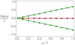
(a) Re($\omega$) at $H/T^{2}=0$

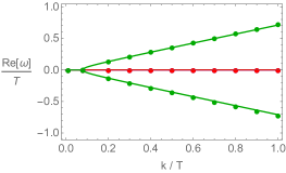
(b) Re($\omega$) at $H/T^{2}=5$

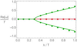
(c) Re($\omega$) at $H/T^{2}=10$

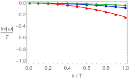
(d) Im($\omega$) at $H/T^{2}=0$

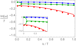
(e) Im($\omega$) at $H/T^{2}=5$

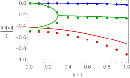
(f) Im($\omega$) at $H/T^{2}=10$

Figure 1: Quasi-normal modes vs dispersion relations from hydrodynamics at zero density ($\mu/T=0$). Left: (a) and (d) at $H/T^{2}=0$. Center: (b) and (e) at $H/T^{2}=5$. Right: (c) and (f) at $H/T^{2}=10$. All figures: colored dots are numerically computed quasi-normal modes and solid lines are dispersion relations from hydrodynamics by (11).

For the $H=0$ case, (a) and (d), the green data corresponds to the sound mode (16), the red data is the charge diffusion mode (18), and the blue data is the shear diffusion mode (18).

For the finite $H$ case, (b) and (e) (or (c) and (f)), the green data consists two dispersions (17): the energy diffusion mode (gapless mode), the cyclotron mode (gapped mode). The red data is another cyclotron mode (19) and the blue data is the sub-diffusion mode (19).

Note that quasi-normal modes have the deviation from dispersion relations of hydrodynamics as the magnetic field increases, e.g., see the cyclotron mode (green or red) in (f). This implies that dispersion relations of hydrodynamics is supposed to be valid in the coherent regime in which the momentum dissipation rate $\Gamma$ (the damping frequency in cyclotron mode (19)) is small as $\Gamma/T\ll 1$ (or $H/T\ll 1$) Hartnoll:2007ih ; Hartnoll:2007ip ; Kim:2015wba ; Blake:2015hxa : the same argument also applies to the case where the energy diffusion mode appears due to the scalar (axion) field Davison:2014lua , i.e., $m/T\ll 1$, $m$ is the coefficient from the scalar field. Note also that the red and green data in Fig. 1 are the reproduction of Jeong:2021zhz .

Quasi-normal modes at finite density:

Next, let us discuss the case at finite density. We display the representative quasi-normal mode data at $\mu/T=5$ at Fig. 2 and compare them with dispersion relations from hydrodynamics: see also Table. 2.

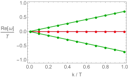
(a) Re($\omega$) at $H/T^{2}=0$

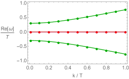
(b) Re($\omega$) at $H/T^{2}=5$

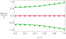
(c) Re($\omega$) at $H/T^{2}=10$

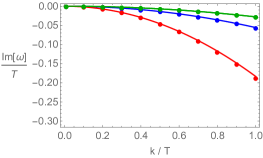
(d) Im($\omega$) at $H/T^{2}=0$

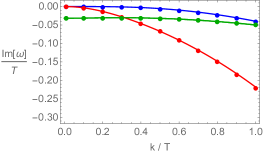
(e) Im($\omega$) at $H/T^{2}=5$

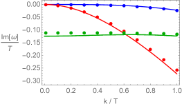
(f) Im($\omega$) at $H/T^{2}=10$

Figure 2: Quasi-normal modes vs dispersion relations from hydrodynamics at finite density ($\mu/T=5$). Left: (a) and (d) at $H/T^{2}=0$. Center: (b) and (e) at $H/T^{2}=5$. Right: (c) and (f) at $H/T^{2}=10$. All figures: colored dots are numerically computed quasi-normal modes and solid lines are dispersion relations from hydrodynamics by (11).

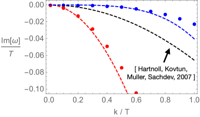
Figure 3: Gapless modes at $\mu/T=5$, $H/T^{2}=10$: Fig. 2(f). All dots are quasi-normal modes. Red dashed line is the diffusion mode (24) and the blue dashed line is sub-diffusion mode (25). Black dashed line is the diffusion mode given in Hartnoll:2007ih .

For $H=0$, (a) and (d), the green and red data correspond to (21) and (22), respectively. The blue data is the shear diffusion mode (23). For $H\neq 0$, (b) and (e), (or (c) and (f)) have the diffusion mode (24) (red data), the sub-diffusion mode (25) (blue data), and the cyclotron mode (25) (green data). Note that, as in the zero density case, quasi-normal modes are well approximated with hydrodynamics at small magnetic fields. Note also that the cyclotron mode at finite density has a real gap as well as an imaginary gap.

As we demonstrated in the section 2, the prefactor ${\left(\frac{\partial{\rho}}{\partial{\mu}}\right)_{T}}$ of the diffusion mode (24) in its numerator was not shown in Hartnoll:2007ih . Thus, it will be instructive to compare (24) with the one given in Hartnoll:2007ih . See Fig. 3. One can find that the prefactor is important to match quasi-normal modes with hydrodynamics.

3.4 Diffusion bounds at finite density

We close this section with the investigation of the transport properties of the gapless modes: the diffusion constant from the diffusion mode (24) and the sub-diffusion constant from the sub-diffusion mode (25). In particular, we focus on the bound of the diffusion constants. It was proposed Blake:2016wvh ; Blake:2016sud that the diffusion constant $D$ may have the lower bound as

$$\begin{split}D\geq v_{B}^{2}/\lambda_{L}\,,\end{split}$$ (42)

which is associated with the properties from quantum chaos Shenker:2013pqa ; Blake:2016wvh ; Roberts:2014isa ; Roberts:2016wdl :

$$\begin{split}v_{B}^{2}=\frac{\pi T}{r_{h}}\,,\quad\lambda_{L}=2\pi T\,,\end{split}$$ (43)

where $v_{B}$ is the butterfly velocity and $\lambda_{L}$ is the Lyapunov exponent. The proposal (42) has been checked in many models Lucas:2018wsc ; Davison:2018ofp ; Gu:2017njx ; Ling:2017jik ; Gu:2017ohj ; Baggioli:2016pia ; Blake:2016jnn ; Blake:2017qgd ; Wu:2017mdl ; Li:2019bgc ; Ge:2017fix ; Li:2017nxh ; Ahn:2017kvc ; Baggioli:2017ojd ; Kim:2017dgz ; Baggioli:2020ljz ; Jeong:2021zhz .

In Fig. 4, we found that the diffusion constant from (24) can respect the lower bound (42) in the presence of both a density and a magnetic field, while the sub-diffusion constant $D_{\text{shear}}:=\frac{\eta}{H^{2}\left(\frac{\partial\rho}{\partial\mu}\right)_{T}}$ in (25) may not.

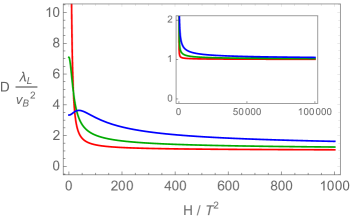
(a) $D$ is from (24)

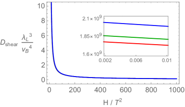
(b) $D_{\text{shear}}$ is from (25)

Figure 4: Diffusion bounds at $\mu/T=(0,3,5)$ (red, green, blue). The diffusion constant $D$ can have the lower bound (42) at $H/T^{2}\gg 1$, while the sub-diffusion constant $D_{\text{shear}}$ does not.

Note that the neutral case (red data) in Fig. 4(a), is the reproduction for the result in Jeong:2021zhz .

Further comments on the diffusion constant:

We make two further comments on the diffusion constant $D$ in (24). First, it is instructive to check if $D$ is related to the energy diffusion constant $D_{E}$ at finite density, since $D$ at zero density was found to be the same as $D_{E}$ Jeong:2021zhz . The energy diffusion constant for the dyonic black hole was given Blake:2017qgd ; Blake:2015hxa as follows

$$\begin{split}D_{E}=\frac{\kappa}{c_{\rho}}\,,\quad\kappa=\frac{s^{2}TH^{2}}{H^{4}+\rho^{2}H^{2}}\,,\quad c_{\rho}=T\left(\frac{\partial s}{\partial T}\right)_{\rho}\,,\end{split}$$ (44)

where thermodynamic quantities are (29).

In Fig. 5, we display both the diffusion constant in (24) and the energy diffusion constant (44) at finite density.

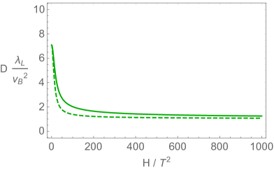
Figure 5: Diffusion bounds at $\mu/T=3$. Solid line is from (24) and dashed line is from (44).

One can see that the diffusion (a solid line), (24), is different from the energy diffusion (a dashed line), (44), in general at finite density.

Note that $D_{E}$ could be finite even at vanishing magnetic field (i.e., translational invariance is not broken) when the system has a density, since $\kappa$ in (44) at $H\rightarrow 0$ is finite if $\rho\neq 0$. Note also that $D\sim D_{E}$ at $H/T^{2}\gg 1$ may be consistent with Blake:2017qgd stating that the diffusion process is governed by the energy diffusion in the low temperature limit of finite density fixed points.

Second, from the recent development of quantum chaos, it was also suggested Blake:2018leo that the lower bound of the diffusion constant, (42), may be associated with the phenomena from the ill-defined Green’s function, called pole-skipping Grozdanov:2017ajz ; Blake:2017ris ; Blake:2018leo . In particular, pole-skipping states that there is a special point in the momentum space as

$$\begin{split}\omega=\omega_{*}\,,\quad k=k_{*}\,,\end{split}$$ (45)

in which the Green’s function $G(\omega_{*},k_{*})\sim\frac{0}{0}$, i.e., ill-defined or not uniquely determined.

In Jeong:2021zhz , it has been found that the leading pole-skipping point (45) of the gravitational sound channel for the generic holographic model including the dyonic black holes (26) is

$$\begin{split}\omega_{*}=i\,\lambda_{L}\,,\quad k_{*}=i\,\frac{\lambda_{L}}{v_{B}}\,,\end{split}$$ (46)

where the quantum choas properties are (43). With (46), the lower bound of the diffusion constant (42) was realized by that the hydrodynamic diffusion mode, $\omega=-iDk^{2}$, e.g. (24), is passing through the pole-skipping point (46) at low temperature as

$$\begin{split}\omega_{*}=-i\,D\,k_{*}^{2}\quad\rightarrow\quad D=v_{B}^{2}/\lambda_{L}\,.\end{split}$$ (47)

To the best of our knowledge, the pole-skipping argument (47) for the lower bound of the diffusion constant only has been confirmed at zero density cases in literature: the energy diffusion with the axion model Blake:2018leo or with a magnetic field Jeong:2021zhz , the crystal diffusion Jeong:2021zhz .

Thus, in order to develop the proposal (47) further, it will be important to check if such an argument holds even at finite density. For this purpose, we investigate if the lower bound of the diffusion constant found in Fig. 4 can be related to the pole-skipping (46).

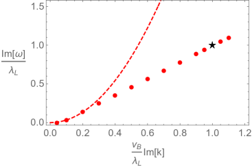
(a) $H/T^{2}=10$

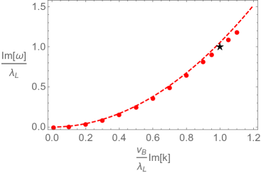
(b) $H/T^{2}=10000$

Figure 6: Pole-skipping and diffusive mode at $\mu/T=5$. All dots are quasi-normal mode, a dashed line is (24), and the star is the pole-skipping point (46).

In Fig. 6, we find that the pole-skipping argument (47) holds even at finite density: as $H/T^{2}\gg 1$ (low temperature limit) from Fig. 6(a) to Fig. 6(b), the pole-skipping point (46) is passing through the diffusive mode (24). One may consider Fig. 6 to be a direct generalization of Jeong:2021zhz to the case of a finite density.

4 Conclusion

We have studied the quasi-normal modes of the dyonic black holes in (3+1) dimensions. In particular, we also revisited the Hartnoll-Kovtun-Müller-Sachdev (HKMS) magneto-hydrodynamics in (2+1) dimensions Hartnoll:2007ih and checked that the quasi-normal modes of dyonic black holes are consistent with the dispersion relations from HKMS magneto-hydrodynamics.

Furthermore, from the detailed analysis of the HKMS magneto-hydrodynamics we slightly corrected the dispersion relation given in previous literature Hartnoll:2007ih , which is important for the matching with quasi-normal modes. Within the quasi-normal mode computations in holography, we also found the relevant independent fluctuation variables (35) of the dyonic black holes, which was not present in previous literature. For the summary of the dispersions of dyonic black holes, see Table. 1 (the neutral case) and Table. 2 (finite density case).

Our work not only provides another successful example showing the consistency between quasi-normal modes in (3+1) dimensions and the hydrodynamic predictions in (2+1) dimensions along the line of Davison:2014lua ; Amoretti:2017frz ; Andrade:2017cnc ; Amoretti:2018tzw ; Ammon:2019wci ; Amoretti:2019cef ; Amoretti:2019kuf ; Baggioli:2021xuv ; Jeong:2021zhz ; Amado:2009ts ; Herzog:2009md ; Yarom:2009uq ; Herzog:2011ec ; Amado:2013xya ; Amado:2013aea ; Esposito:2016ria ; Arean:2021tks ; Ammon:2021slb in holography, but also is useful for the complete understanding of the dyonic black holes in that our work extends the previous works, the thermodynamic properties or the transport properties at zero wave vector, of the dyonic black holes Hartnoll:2007ih ; Hartnoll:2007ip ; Hartnoll:2007ai ; Herzog:2007ij ; Denef:2009yy ; OBannon:2007in ; Buchbinder:2008dc ; Buchbinder:2009aa ; Buchbinder:2009mk ; Bergman:2012na ; Gubankova:2013lca ; Dutta:2013dca ; Kim:2015wba ; Amoretti:2015gna ; Blake:2015ina ; Lucas:2015pxa ; Zhou:2015dha ; Davison:2015bea ; Blake:2015hxa ; Donos:2015bxe ; Seo:2015pug ; Ahn:2015shg ; Amoretti:2016cad ; Kim:2016hzi ; Ge:2016sel ; Khimphun:2017mqb ; Blake:2017qgd ; Cremonini:2017qwq ; Seo:2017yux ; Chen:2017gsl ; Blauvelt:2017koq ; Angelinos:2018qlc ; Pal:2019bfw ; Kim:2019lxb ; Hoyos:2019pyz ; Song:2019rnf ; Amoretti:2019buu ; Baggioli:2020edn ; An:2020tkn ; Kim:2020ozm22 ; Amoretti:2020mkp ; Amoretti:2021lll ; Amoretti:2021fch ; Jokela:2021uws ; Priyadarshinee:2021rch for the case at finite wave vector.

In addition to matching quasi-normal modes with the hydrodynamic theory, we also investigated the transport property at finite wave vector: the diffusion constant. We found that the diffusion constant from the dyonic black hole can have a lower bound at low temperature and show that such a lower bound can also be understood as the pole-skipping. In particular, our work confirmed the relation between the diffusion bound and pole-skipping at a finite density for the first time.

One of the interesting future directions from this paper will be to investigate the dynamical gauge fields of dyonic black holes. In particular, following Hernandez:2017mch considering the (3+1) dimensional hydrodynamics of the dynamical gauge fields, one can also study the (2+1) dimensional hydrodynamics together with the dynamical gauge field and compare it with the quasi-normal modes of dyonic black holes wipYW3 .

It may also be interesting to study the quasi-normal modes of the dyonic black holes in the presence of the explicitly broken translational invariance. For instance, the dyonic black holes with the axion model Kim:2015wba produce the DC conductivities (i.e., zero wave vector property)

$$\begin{split}(m=0):\quad&\sigma^{xx}_{DC}=\sigma^{yy}_{DC}=0\,,\qquad\qquad\,\,\,\,\sigma^{xy}_{DC}=-\sigma^{yx}_{DC}=\frac{\rho}{H}\,,\\ (H=0):\quad&\sigma^{xx}_{DC}=\sigma^{yy}_{DC}=1+\frac{\mu^{2}}{m^{2}}\,,\qquad\sigma^{xy}_{DC}=-\sigma^{yx}_{DC}=0\,,\\ \end{split}$$ (48)

where $m$ is the strength of the translational symmetry breaking, $H$ is the magnetic field. One can see that the two limits given in (48) do not commute. This implies that magneto-hydrodynamics with the broken translational symmetry may also give different dispersion relations (i.e., the finite wave vector property) depending on whether we take $m=0$ first or $H=0$ first. Thus, the interplay between HKMS magneto-hydrodynamics, the first line in (48), and hydrodynamics with broken translational invariance, the second line in (48), may not be a trivial subject. Note that one can also study similar topics with spontaneously broken symmetry Baggioli:2020edn . We leave these subject as future work and hope to address it in the near future.

- (1) S. A. Hartnoll, A. Lucas and S. Sachdev, Holographic quantum matter, 1612.07324.
- (2) J. Zaanen, Y.-W. Sun, Y. Liu and K. Schalm, Holographic Duality in Condensed Matter Physics. Cambridge Univ. Press, 2015.
- (3) M. Ammon and J. Erdmenger, Gauge/gravity duality. Cambridge Univ. Pr., Cambridge, UK, 2015.
- (4) M. Baggioli, Applied Holography: A Practical Mini-Course. SpringerBriefs in Physics. Springer, 2019, 10.1007/978-3-030-35184-7.
- (5) S. A. Hartnoll, P. K. Kovtun, M. Muller and S. Sachdev, Theory of the Nernst effect near quantum phase transitions in condensed matter, and in dyonic black holes, Phys.Rev. B76 (2007) 144502, [0706.3215].
- (6) P. Basu, A. Mukherjee and H.-H. Shieh, Supercurrent: Vector Hair for an AdS Black Hole, Phys. Rev. D 79 (2009) 045010, [0809.4494].
- (7) C. P. Herzog, P. K. Kovtun and D. T. Son, Holographic model of superfluidity, Phys. Rev. D 79 (2009) 066002, [0809.4870].
- (8) S. A. Hartnoll, C. P. Herzog and G. T. Horowitz, Building a Holographic Superconductor, Phys.Rev.Lett. 101 (2008) 031601, [0803.3295].
- (9) S. A. Hartnoll, C. P. Herzog and G. T. Horowitz, Holographic Superconductors, JHEP 0812 (2008) 015, [0810.1563].
- (10) H.-S. Jeong and K.-Y. Kim, Homes’ law in holographic superconductor with linear- resistivity, 2112.01153.
- (11) M. Baggioli and G. Frangi, Holographic Supersolids, 2202.03745.
- (12) R. A. Davison and B. Goutéraux, Momentum dissipation and effective theories of coherent and incoherent transport, JHEP 01 (2015) 039, [1411.1062].
- (13) A. Amoretti, D. Areán, B. Goutéraux and D. Musso, Effective holographic theory of charge density waves, Phys. Rev. D97 (2018) 086017, [1711.06610].
- (14) T. Andrade, M. Baggioli, A. Krikun and N. Poovuttikul, Pinning of longitudinal phonons in holographic spontaneous helices, JHEP 02 (2018) 085, [1708.08306].
- (15) A. Amoretti, D. Areán, B. Goutéraux and D. Musso, Universal relaxation in a holographic metallic density wave phase, Phys. Rev. Lett. 123 (2019) 211602, [1812.08118].
- (16) M. Ammon, M. Baggioli and A. Jiménez-Alba, A Unified Description of Translational Symmetry Breaking in Holography, JHEP 09 (2019) 124, [1904.05785].
- (17) A. Amoretti, D. Areán, B. Goutéraux and D. Musso, Diffusion and universal relaxation of holographic phonons, JHEP 10 (2019) 068, [1904.11445].
- (18) A. Amoretti, D. Areán, B. Goutéraux and D. Musso, Gapless and gapped holographic phonons, JHEP 01 (2020) 058, [1910.11330].
- (19) M. Baggioli, K.-Y. Kim, L. Li and W.-J. Li, Holographic Axion Model: a simple gravitational tool for quantum matter, Sci. China Phys. Mech. Astron. 64 (2021) 270001, [2101.01892].
- (20) H.-S. Jeong, K.-Y. Kim and Y.-W. Sun, Bound of diffusion constants from pole-skipping points: spontaneous symmetry breaking and magnetic field, JHEP 07 (2021) 105, [2104.13084].
- (21) I. Amado, M. Kaminski and K. Landsteiner, Hydrodynamics of Holographic Superconductors, JHEP 0905 (2009) 021, [0903.2209].
- (22) C. P. Herzog and A. Yarom, Sound modes in holographic superfluids, Phys. Rev. D 80 (2009) 106002, [0906.4810].
- (23) A. Yarom, Fourth sound of holographic superfluids, JHEP 07 (2009) 070, [0903.1353].
- (24) C. P. Herzog, N. Lisker, P. Surowka and A. Yarom, Transport in holographic superfluids, JHEP 08 (2011) 052, [1101.3330].
- (25) I. Amado, D. Arean, A. Jimenez-Alba, K. Landsteiner, L. Melgar and I. S. Landea, Holographic Type II Goldstone bosons, JHEP 07 (2013) 108, [1302.5641].
- (26) I. Amado, D. Areán, A. Jiménez-Alba, K. Landsteiner, L. Melgar and I. Salazar Landea, Holographic Superfluids and the Landau Criterion, JHEP 02 (2014) 063, [1307.8100].
- (27) A. Esposito, S. Garcia-Saenz and R. Penco, First sound in holographic superfluids at zero temperature, JHEP 12 (2016) 136, [1606.03104].
- (28) D. Arean, M. Baggioli, S. Grieninger and K. Landsteiner, A holographic superfluid symphony, JHEP 11 (2021) 206, [2107.08802].
- (29) M. Ammon, D. Arean, M. Baggioli, S. Gray and S. Grieninger, Pseudo-spontaneous Symmetry Breaking in Hydrodynamics and Holography, 2111.10305.
- (30) M. Blake, R. A. Davison, S. Grozdanov and H. Liu, Many-body chaos and energy dynamics in holography, JHEP 10 (2018) 035, [1809.01169].
- (31) D. Arean, R. A. Davison, B. Goutéraux and K. Suzuki, Hydrodynamic diffusion and its breakdown near AdS2 fixed points, 2011.12301.
- (32) N. Wu, M. Baggioli and W.-J. Li, On the universality of AdS2 diffusion bounds and the breakdown of linearized hydrodynamics, JHEP 05 (2021) 014, [2102.05810].
- (33) H.-S. Jeong, K.-Y. Kim and Y.-W. Sun, The breakdown of magneto-hydrodynamics near AdS2 fixed point and energy diffusion bound, JHEP 02 (2022) 006, [2105.03882].
- (34) K.-B. Huh, H.-S. Jeong, K.-Y. Kim and Y.-W. Sun, Upper bound of the charge diffusion constant in holography, 2111.07515.
- (35) Y. Liu and X.-M. Wu, Breakdown of hydrodynamics from holographic pole collision, JHEP 01 (2022) 155, [2111.07770].
- (36) S. A. Hartnoll and C. P. Herzog, Ohm’s Law at strong coupling: S duality and the cyclotron resonance, Phys.Rev. D76 (2007) 106012, [0706.3228].
- (37) S. A. Hartnoll and P. Kovtun, Hall conductivity from dyonic black holes, Phys.Rev. D76 (2007) 066001, [0704.1160].
- (38) C. P. Herzog, P. Kovtun, S. Sachdev and D. T. Son, Quantum critical transport, duality, and M-theory, Phys.Rev. D75 (2007) 085020, [hep-th/0701036].
- (39) F. Denef, S. A. Hartnoll and S. Sachdev, Quantum oscillations and black hole ringing, Phys. Rev. D80 (2009) 126016, [0908.1788].
- (40) A. O’Bannon, Hall Conductivity of Flavor Fields from AdS/CFT, Phys. Rev. D76 (2007) 086007, [0708.1994].
- (41) E. I. Buchbinder, S. E. Vazquez and A. Buchel, Sound Waves in (2+1) Dimensional Holographic Magnetic Fluids, JHEP 12 (2008) 090, [0810.4094].
- (42) E. I. Buchbinder, Fate of sound and diffusion in a holographic magnetic field, Physical Review D 79 (2009) .
- (43) E. I. Buchbinder and A. Buchel, Relativistic Conformal Magneto-Hydrodynamics from Holography, Phys. Lett. B 678 (2009) 135–138, [0902.3170].
- (44) O. Bergman, J. Erdmenger and G. Lifschytz, A Review of Magnetic Phenomena in Probe-Brane Holographic Matter, Lect. Notes Phys. 871 (2013) 591–624, [1207.5953].
- (45) E. Gubankova, J. Brill, M. Cubrovic, K. Schalm, P. Schijven and J. Zaanen, Holographic description of strongly correlated electrons in external magnetic fields, Lect. Notes Phys. 871 (2013) 555–589, [1304.3835].
- (46) S. Dutta, A. Jain and R. Soni, Dyonic Black Hole and Holography, JHEP 12 (2013) 060, [1310.1748].
- (47) K.-Y. Kim, K. K. Kim, Y. Seo and S.-J. Sin, Thermoelectric Conductivities at Finite Magnetic Field and the Nernst Effect, JHEP 07 (2015) 027, [1502.05386].
- (48) A. Amoretti and D. Musso, Magneto-transport from momentum dissipating holography, JHEP 09 (2015) 094, [1502.02631].
- (49) M. Blake, A. Donos and N. Lohitsiri, Magnetothermoelectric Response from Holography, JHEP 08 (2015) 124, [1502.03789].
- (50) A. Lucas and S. Sachdev, Memory matrix theory of magnetotransport in strange metals, Phys. Rev. B 91 (2015) 195122, [1502.04704].
- (51) Z. Zhou, J.-P. Wu and Y. Ling, DC and Hall conductivity in holographic massive Einstein-Maxwell-Dilaton gravity, JHEP 08 (2015) 067, [1504.00535].
- (52) R. A. Davison and B. Goutéraux, Dissecting holographic conductivities, JHEP 09 (2015) 090, [1505.05092].
- (53) M. Blake, Magnetotransport from the fluid/gravity correspondence, JHEP 10 (2015) 078, [1507.04870].
- (54) A. Donos, J. P. Gauntlett, T. Griffin and L. Melgar, DC Conductivity of Magnetised Holographic Matter, JHEP 01 (2016) 113, [1511.00713].
- (55) Y. Seo, K.-Y. Kim, K. K. Kim and S.-J. Sin, Character of matter in holography: Spin–orbit interaction, Phys. Lett. B 759 (2016) 104–109, [1512.08916].
- (56) B. Ahn, S. Hyun, K. K. Kim, S.-A. Park and S.-H. Yi, Holography without counter terms, Phys. Rev. D 94 (2016) 024043, [1512.09319].
- (57) A. Amoretti, M. Baggioli, N. Magnoli and D. Musso, Chasing the cuprates with dilatonic dyons, JHEP 06 (2016) 113, [1603.03029].
- (58) K. K. Kim, M. Park and K.-Y. Kim, Ward identity and Homes’ law in a holographic superconductor with momentum relaxation, JHEP 10 (2016) 041, [1604.06205].
- (59) X.-H. Ge, Y. Tian, S.-Y. Wu and S.-F. Wu, Hyperscaling violating black hole solutions and Magneto-thermoelectric DC conductivities in holography, Phys. Rev. D96 (2017) 046015, [1606.05959].
- (60) S. Khimphun, B.-H. Lee, C. Park and Y.-L. Zhang, Anisotropic dyonic black brane and its effects on holographic conductivity, JHEP 10 (2017) 064, [1705.00862].
- (61) M. Blake, R. A. Davison and S. Sachdev, Thermal diffusivity and chaos in metals without quasiparticles, Phys. Rev. D 96 (2017) 106008, [1705.07896].
- (62) S. Cremonini, A. Hoover and L. Li, Backreacted DBI Magnetotransport with Momentum Dissipation, JHEP 10 (2017) 133, [1707.01505].
- (63) Y. Seo, G. Song, C. Park and S.-J. Sin, Small Fermi Surfaces and Strong Correlation Effects in Dirac Materials with Holography, JHEP 10 (2017) 204, [1708.02257].
- (64) Z.-N. Chen, X.-H. Ge, S.-Y. Wu, G.-H. Yang and H.-S. Zhang, Magnetothermoelectric DC conductivities from holography models with hyperscaling factor in Lifshitz spacetime, Nucl. Phys. B924 (2017) 387–405, [1709.08428].
- (65) E. Blauvelt, S. Cremonini, A. Hoover, L. Li and S. Waskie, Holographic model for the anomalous scalings of the cuprates, Phys. Rev. D97 (2018) 061901, [1710.01326].
- (66) N. Angelinos, Criticality and Transport in Magnetized Holographic Systems, other thesis, 2018, 12, 2018.
- (67) S. S. Pal, Thermal and thermoelectric conductivity of Einstein-DBI system, Eur. Phys. J. C 80 (2020) 225, [1901.07175].
- (68) K. K. Kim, K.-Y. Kim, Y. Seo and S.-J. Sin, Building magnetic hysteresis in holography, JHEP 07 (2019) 158, [1902.10929].
- (69) C. Hoyos, F. Peña Benitez and P. Witkowski, Hall Viscosity in a Strongly Coupled Magnetized Plasma, JHEP 08 (2019) 146, [1906.04752].
- (70) G. Song, Y. Seo, K.-Y. Kim and S.-J. Sin, Interaction induced quasi-particle spectrum in holography, JHEP 11 (2019) 103, [1907.06188].
- (71) A. Amoretti, M. Meinero, D. K. Brattan, F. Caglieris, E. Giannini, M. Affronte et al., Hydrodynamical description for magneto-transport in the strange metal phase of Bi-2201, Phys. Rev. Res. 2 (2020) 023387, [1909.07991].
- (72) M. Baggioli, S. Grieninger and L. Li, Magnetophonons & type-B Goldstones from Hydrodynamics to Holography, JHEP 09 (2020) 037, [2005.01725].
- (73) Y.-S. An, T. Ji and L. Li, Magnetotransport and Complexity of Holographic Metal-Insulator Transitions, JHEP 10 (2020) 023, [2007.13918].
- (74) K. K. Kim, K.-Y. Kim, S.-J. Sin and Y. Seo, Impurity effect on hysteric magnetoconductance: holographic approach, JHEP 11 (2021) 046, [2008.13147].
- (75) A. Amoretti, D. K. Brattan, N. Magnoli and M. Scanavino, Magneto-thermal transport implies an incoherent Hall conductivity, JHEP 08 (2020) 097, [2005.09662].
- (76) A. Amoretti, D. Arean, D. K. Brattan and L. Martinoia, Hydrodynamic magneto-transport in holographic charge density wave states, JHEP 11 (2021) 011, [2107.00519].
- (77) A. Amoretti, D. Arean, D. K. Brattan and N. Magnoli, Hydrodynamic magneto-transport in charge density wave states, 2101.05343.
- (78) N. Jokela, M. Järvinen and M. Lippert, Novel semi-circle law and Hall sliding in a strongly interacting electron liquid, 2111.14885.
- (79) S. Priyadarshinee, S. Mahapatra and I. Banerjee, Analytic topological hairy dyonic black holes and thermodynamics, Phys. Rev. D 104 (2021) 084023, [2108.02514].
- (80) M. Edalati, J. I. Jottar and R. G. Leigh, Holography and the sound of criticality, JHEP 10 (2010) 058, [1005.4075].
- (81) R. A. Davison and N. K. Kaplis, Bosonic excitations of the Reissner-Nordstrom black hole, JHEP 12 (2011) 037, [1111.0660].
- (82) N. I. Gushterov, A. O’Bannon and R. Rodgers, Holographic Zero Sound from Spacetime-Filling Branes, JHEP 10 (2018) 076, [1807.11327].
- (83) M. Baggioli, U. Gran and M. Tornsö, Collective modes of polarizable holographic media in magnetic fields, JHEP 06 (2021) 014, [2102.09969].
- (84) A. Donos, C. Pantelidou and V. Ziogas, Incoherent hydrodynamics of density waves in magnetic fields, JHEP 05 (2021) 270, [2101.06230].
- (85) L. V. Delacrétaz, B. Goutéraux, S. A. Hartnoll and A. Karlsson, Theory of collective magnetophonon resonance and melting of a field-induced Wigner solid, Phys. Rev. B 100 (2019) 085140, [1904.04872].
- (86) D. K. Brattan, R. A. Davison, S. A. Gentle and A. O’Bannon, Collective Excitations of Holographic Quantum Liquids in a Magnetic Field, JHEP 11 (2012) 084, [1209.0009].
- (87) S. Janiszewski and M. Kaminski, Quasinormal modes of magnetic and electric black branes versus far from equilibrium anisotropic fluids, Phys. Rev. D93 (2016) 025006, [1508.06993].
- (88) M. Ammon, S. Grieninger, A. Jimenez-Alba, R. P. Macedo and L. Melgar, Holographic quenches and anomalous transport, JHEP 09 (2016) 131, [1607.06817].
- (89) M. Ammon, M. Kaminski, R. Koirala, J. Leiber and J. Wu, Quasinormal modes of charged magnetic black branes & chiral magnetic transport, JHEP 04 (2017) 067, [1701.05565].
- (90) M. Ammon, S. Grieninger, J. Hernandez, M. Kaminski, R. Koirala, J. Leiber et al., Chiral hydrodynamics in strong external magnetic fields, JHEP 04 (2021) 078, [2012.09183].
- (91) A. Gromov, A. Lucas and R. M. Nandkishore, Fracton hydrodynamics, Phys. Rev. Res. 2 (2020) 033124, [2003.09429].
- (92) P. K. Kovtun and A. O. Starinets, Quasinormal modes and holography, Phys. Rev. D72 (2005) 086009, [hep-th/0506184].
- (93) C. P. Herzog, The Hydrodynamics of M theory, JHEP 12 (2002) 026, [hep-th/0210126].
- (94) M. Edalati, J. I. Jottar and R. G. Leigh, Shear Modes, Criticality and Extremal Black Holes, JHEP 04 (2010) 075, [1001.0779].
- (95) R. A. Davison and A. Parnachev, Hydrodynamics of cold holographic matter, JHEP 06 (2013) 100, [1303.6334].
- (96) R. A. Davison, Momentum relaxation in holographic massive gravity, Phys.Rev. D88 (2013) 086003, [1306.5792].
- (97) M. Kaminski, K. Landsteiner, J. Mas, J. P. Shock and J. Tarrio, Holographic Operator Mixing and Quasinormal Modes on the Brane, JHEP 1002 (2010) 021, [0911.3610].
- (98) P. Kovtun, D. T. Son and A. O. Starinets, Viscosity in strongly interacting quantum field theories from black hole physics, Phys. Rev. Lett. 94 (2005) 111601, [hep-th/0405231].
- (99) P. Kovtun, D. T. Son and A. O. Starinets, Holography and hydrodynamics: Diffusion on stretched horizons, JHEP 0310 (2003) 064, [hep-th/0309213].
- (100) R. A. Davison, B. Goutéraux and S. A. Hartnoll, Incoherent transport in clean quantum critical metals, JHEP 10 (2015) 112, [1507.07137].
- (101) A. Lucas, Conductivity of a strange metal: from holography to memory functions, JHEP 03 (2015) 071, [1501.05656].
- (102) S. A. Hartnoll, D. M. Ramirez and J. E. Santos, Entropy production, viscosity bounds and bumpy black holes, JHEP 03 (2016) 170, [1601.02757].
- (103) L. Alberte, M. Ammon, A. Jiménez-Alba, M. Baggioli and O. Pujolàs, Holographic Phonons, Phys. Rev. Lett. 120 (2018) 171602, [1711.03100].
- (104) L. Alberte, M. Ammon, M. Baggioli, A. Jimnez and O. Pujol s, Black hole elasticity and gapped transverse phonons in holography, JHEP 01 (2018) 129, [1708.08477].
- (105) M. Baggioli and A. Buchel, Holographic Viscoelastic Hydrodynamics, JHEP 03 (2019) 146, [1805.06756].
- (106) L. Alberte, M. Baggioli, A. Khmelnitsky and O. Pujolas, Solid Holography and Massive Gravity, JHEP 02 (2016) 114, [1510.09089].
- (107) L. Alberte, M. Baggioli and O. Pujolas, Viscosity bound violation in holographic solids and the viscoelastic response, JHEP 07 (2016) 074, [1601.03384].
- (108) P. Burikham and N. Poovuttikul, Shear viscosity in holography and effective theory of transport without translational symmetry, Phys. Rev. D94 (2016) 106001, [1601.04624].
- (109) T. Ciobanu and D. M. Ramirez, Shear hydrodynamics, momentum relaxation, and the KSS bound, 1708.04997.
- (110) N. Iqbal and H. Liu, Universality of the hydrodynamic limit in AdS/CFT and the membrane paradigm, Phys. Rev. D79 (2009) 025023, [0809.3808].
- (111) S. Jain, R. Samanta and S. P. Trivedi, The Shear Viscosity in Anisotropic Phases, JHEP 10 (2015) 028, [1506.01899].
- (112) S. I. Finazzo, R. Critelli, R. Rougemont and J. Noronha, Momentum transport in strongly coupled anisotropic plasmas in the presence of strong magnetic fields, Phys. Rev. D 94 (2016) 054020, [1605.06061].
- (113) A. Rebhan and D. Steineder, Violation of the Holographic Viscosity Bound in a Strongly Coupled Anisotropic Plasma, Phys. Rev. Lett. 108 (2012) 021601, [1110.6825].
- (114) D. Giataganas, Observables in Strongly Coupled Anisotropic Theories, PoS Corfu2012 (2013) 122, [1306.1404].
- (115) M. Blake, Universal Charge Diffusion and the Butterfly Effect in Holographic Theories, Phys. Rev. Lett. 117 (2016) 091601, [1603.08510].
- (116) M. Blake, Universal Diffusion in Incoherent Black Holes, Phys. Rev. D94 (2016) 086014, [1604.01754].
- (117) S. H. Shenker and D. Stanford, Black holes and the butterfly effect, JHEP 03 (2014) 067, [1306.0622].
- (118) D. A. Roberts, D. Stanford and L. Susskind, Localized shocks, JHEP 03 (2015) 051, [1409.8180].
- (119) D. A. Roberts and B. Swingle, Lieb-Robinson Bound and the Butterfly Effect in Quantum Field Theories, Phys. Rev. Lett. 117 (2016) 091602, [1603.09298].
- (120) A. Lucas, Operator size at finite temperature and Planckian bounds on quantum dynamics, Phys. Rev. Lett. 122 (2019) 216601, [1809.07769].
- (121) R. A. Davison, S. A. Gentle and B. Goutéraux, Slow relaxation and diffusion in holographic quantum critical phases, Phys. Rev. Lett. 123 (2019) 141601, [1808.05659].
- (122) Y. Gu, A. Lucas and X.-L. Qi, Spread of entanglement in a Sachdev-Ye-Kitaev chain, JHEP 09 (2017) 120, [1708.00871].
- (123) Y. Ling and Z.-Y. Xian, Holographic Butterfly Effect and Diffusion in Quantum Critical Region, JHEP 09 (2017) 003, [1707.02843].
- (124) Y. Gu, A. Lucas and X.-L. Qi, Energy diffusion and the butterfly effect in inhomogeneous Sachdev-Ye-Kitaev chains, 1702.08462.
- (125) M. Baggioli, B. Goutéraux, E. Kiritsis and W.-J. Li, Higher derivative corrections to incoherent metallic transport in holography, JHEP 03 (2017) 170, [1612.05500].
- (126) M. Blake and A. Donos, Diffusion and Chaos from near AdS2 horizons, JHEP 02 (2017) 013, [1611.09380].
- (127) S.-F. Wu, B. Wang, X.-H. Ge and Y. Tian, Universal diffusion in strange-metal transport, 1702.08803.
- (128) W. Li, S. Lin and J. Mei, Thermal diffusion and quantum chaos in neutral magnetized plasma, Phys. Rev. D 100 (2019) 046012, [1905.07684].
- (129) X.-H. Ge, S.-J. Sin, Y. Tian, S.-F. Wu and S.-Y. Wu, Charged BTZ-like black hole solutions and the diffusivity-butterfly velocity relation, JHEP 01 (2018) 068, [1712.00705].
- (130) W.-J. Li, P. Liu and J.-P. Wu, Weyl corrections to diffusion and chaos in holography, JHEP 04 (2018) 115, [1710.07896].
- (131) H.-S. Jeong, Y. Ahn, D. Ahn, C. Niu, W.-J. Li and K.-Y. Kim, Thermal diffusivity and butterfly velocity in anisotropic Q-Lattice models, JHEP 01 (2018) 140, [1708.08822].
- (132) M. Baggioli and W.-J. Li, Diffusivities bounds and chaos in holographic Horndeski theories, JHEP 07 (2017) 055, [1705.01766].
- (133) K.-Y. Kim and C. Niu, Diffusion and Butterfly Velocity at Finite Density, JHEP 06 (2017) 030, [1704.00947].
- (134) M. Baggioli and W.-J. Li, Universal Bounds on Transport in Holographic Systems with Broken Translations, SciPost Phys. 9 (2020) 007, [2005.06482].
- (135) S. Grozdanov, K. Schalm and V. Scopelliti, Black hole scrambling from hydrodynamics, Phys. Rev. Lett. 120 (2018) 231601, [1710.00921].
- (136) M. Blake, H. Lee and H. Liu, A quantum hydrodynamical description for scrambling and many-body chaos, JHEP 10 (2018) 127, [1801.00010].
- (137) M. Blake, R. A. Davison and D. Vegh, Horizon constraints on holographic Green’s functions, JHEP 01 (2020) 077, [1904.12883].
- (138) S. Grozdanov, P. K. Kovtun, A. O. Starinets and P. Tadić, The complex life of hydrodynamic modes, JHEP 11 (2019) 097, [1904.12862].
- (139) N. Ceplak, K. Ramdial and D. Vegh, Fermionic pole-skipping in holography, JHEP 07 (2020) 203, [1910.02975].
- (140) N. Ceplak and D. Vegh, Pole-skipping and Rarita-Schwinger fields, 2101.01490.
- (141) M. Natsuume and T. Okamura, Holographic chaos, pole-skipping, and regularity, PTEP 2020 (2020) 013B07, [1905.12014].
- (142) M. Natsuume and T. Okamura, Nonuniqueness of Green’s functions at special points, JHEP 12 (2019) 139, [1905.12015].
- (143) M. Natsuume and T. Okamura, Pole-skipping with finite-coupling corrections, Phys. Rev. D 100 (2019) 126012, [1909.09168].
- (144) S. Grozdanov, On the connection between hydrodynamics and quantum chaos in holographic theories with stringy corrections, JHEP 01 (2019) 048, [1811.09641].
- (145) S. Grozdanov, Bounds on transport from univalence and pole-skipping, Phys. Rev. Lett. 126 (2021) 051601, [2008.00888].
- (146) Y. Liu and A. Raju, Quantum Chaos in Topologically Massive Gravity, JHEP 12 (2020) 027, [2005.08508].
- (147) N. Abbasi and S. Tahery, Complexified quasinormal modes and the pole-skipping in a holographic system at finite chemical potential, JHEP 10 (2020) 076, [2007.10024].
- (148) A. Jansen and C. Pantelidou, Quasinormal modes in charged fluids at complex momentum, JHEP 10 (2020) 121, [2007.14418].
- (149) X. Wu, Higher curvature corrections to pole-skipping, JHEP 12 (2019) 140, [1909.10223].
- (150) N. Abbasi and J. Tabatabaei, Quantum chaos, pole-skipping and hydrodynamics in a holographic system with chiral anomaly, JHEP 03 (2020) 050, [1910.13696].
- (151) F. M. Haehl and M. Rozali, Effective Field Theory for Chaotic CFTs, JHEP 10 (2018) 118, [1808.02898].
- (152) S. Das, B. Ezhuthachan and A. Kundu, Real time dynamics from low point correlators in 2d BCFT, JHEP 12 (2019) 141, [1907.08763].
- (153) D. M. Ramirez, Chaos and pole skipping in CFT2, 2009.00500.
- (154) Y. Ahn, V. Jahnke, H.-S. Jeong and K.-Y. Kim, Scrambling in Hyperbolic Black Holes: shock waves and pole-skipping, JHEP 10 (2019) 257, [1907.08030].
- (155) Y. Ahn, V. Jahnke, H.-S. Jeong, K.-Y. Kim, K.-S. Lee and M. Nishida, Pole-skipping of scalar and vector fields in hyperbolic space: conformal blocks and holography, JHEP 09 (2020) 111, [2006.00974].
- (156) Y. Ahn, V. Jahnke, H.-S. Jeong, K.-S. Lee, M. Nishida and K.-Y. Kim, Classifying pole-skipping points, JHEP 03 (2021) 175, [2010.16166].
- (157) C. Choi, M. Mezei and G. Sárosi, Pole skipping away from maximal chaos, 2010.08558.
- (158) K.-Y. Kim, K.-S. Lee and M. Nishida, Holographic scalar and vector exchange in OTOCs and pole-skipping phenomena, JHEP 04 (2021) 092, [2011.13716].
- (159) K. Sil, Pole skipping and chaos in anisotropic plasma: a holographic study, JHEP 03 (2021) 232, [2012.07710].
- (160) N. Abbasi and M. Kaminski, Constraints on quasinormal modes and bounds for critical points from pole-skipping, JHEP 03 (2021) 265, [2012.15820].
- (161) K.-Y. Kim, K.-S. Lee and M. Nishida, Regge conformal blocks from the Rindler-AdS black hole and the pole-skipping phenomena, JHEP 11 (2021) 020, [2105.07778].
- (162) K.-Y. Kim, K.-S. Lee and M. Nishida, Construction of bulk solutions for towers of pole-skipping points, 2112.11662.
- (163) M. Blake and R. A. Davison, Chaos and pole-skipping in rotating black holes, JHEP 01 (2022) 013, [2111.11093].
- (164) S. Mahish and K. Sil, Quantum information scrambling and quantum chaos in little string theory, 2202.05865.
- (165) J. Hernandez and P. Kovtun, Relativistic magnetohydrodynamics, JHEP 05 (2017) 001, [1703.08757].
- (166) Y. Ahn, M. Baggioli, K.-B. Huh, H.-S. Jeong, K.-Y. Kim and Y.-W. Sun, Dynamical gauge fields in holography and hydrodynamics, working in progress (appear soon) .