Why Constant-Composition Codes
Reduce Nonlinear Interference Noise

Abstract

A time-domain perturbation model of the nonlinear Schrödinger equation is used to study wave-length-division multiplexed communication over a single polarization. The model explains (a) why constant-composition codes offer an improvement in signal to noise ratio compared with independent and uniform selection of constellation points and (b) why similar gains are obtained using carrier recovery algorithms even without using constant-composition codes.

I Introduction

Interchannel interference induced by the effects of Kerr nonlinearity is a major factor limiting the information-carrying capacity of wave-length-division-multiplexed (WDM) optical transport networks. At transmission power levels beyond a certain optimum, the harmful effects of nonlinear signal–signal interactions resulting in cross-phase modulation (XPM) outweigh the benefits of transmitting a stronger signal [1, 2]. Designing communication schemes that can tolerate or compensate XPM is under active research [3].

Recent studies on probabilistic shaping for fiber optic systems have reported that a considerable gain in signal-to-noise ratio (SNR) can be achieved in the presence of Kerr nonlinearity using distribution matchers of short blocklength, but that the gain reduces (or is absent) at longer blocklength. In [4], it is shown that finite blocklength enumerative sphere shaping and constant-composition (CC) distribution matching achieve higher effective SNRs than their infinite blocklength counterparts. The same observation is made in [5]. In [6], the effect of a CC distribution matcher on the induced nonlinear interference is attributed to a limited concentration of identical symbols. The effect of blocklength of a distribution matcher on the nonlinear interference noise is further studied in [7]. In [8], the temporal energy behavior of symbol sequences is studied and a new metric, called energy dispersion index, is proposed to predict the impact of blocklength of the distribution matcher on the effective SNR for systems that use a CC distribution matcher for probabilistic shaping. Similar observations, but in a different context, have been reported as early as the work in [9], where it is shown that to estimate the nonlinear interference accurately, longer bit sequences should be simulated, since simulations with shorter bit sequences induce higher SNRs.

While probabilistic shaping with finite-length CC codebooks provides demonstrable improvements in effective SNR in the absence of phase-tracking algorithms at the receiver, the authors of [10] show that, in the nonlinear regime of operation, the gain in generalized mutual information obtained by probabilistic amplitude shaping via enumerative sphere shaping is the same as the gain of typical carrier phase recovery algorithms. In particular, no additional shaping gain is observed when a carrier phase recovery module is in place, which is the case in all practical systems. This observation raises the question of whether or not the SNR gain of short-length distribution matchers is of practical importance.

In this paper, we provide a theoretical justification for the superior performance (in terms of SNR) of short CC codes. Our work is based on the the first order perturbation model of [2]. We determine computationally feasible expressions for the perturbation coefficients of the most dominant XPM terms, and we verify that the dominant XPM coefficients are slowly varying functions of the time-separation of symbols in neighboring channels. Our results show that a more general class of codes, namely spherical codes, have the potential to offer the same gain in SNR as long as their blocklength is not too long. We also explain why carrier phase recovery algorithms can provide similar gains.

The rest of the paper is organized as follows. In Section II, the theory of the first order perturbation method of [2] is reviewed. This section includes a new and efficient method to accurately calculate the most dominant perturbation coefficients. Section III reviews the main properties of CC codes. In Section IV, we use the perturbation model to explain why CC codes offer an SNR gain, and why carrier phase recovery can provide similar gains. Section V concludes the paper.

II A Mathematical Model for Nonlinear Signal–Signal Interactions

In this section, we re-derive the time domain perturbation model of [2]. This model will prove useful in the following sections to investigate the nonlinear interference noise of CC codes.

II-A Channel Model

Propagation of a narrow-band optical signal over a single mode fiber without attenuation is described by the nonlinear Schrödinger (NLS) equation [11]

$$\frac{\partial Q(\tau,l)}{\partial l}=-i\frac{\beta_{2}}{2}\frac{\partial^{2}Q(\tau,l)}{\partial\tau^{2}}+i\gamma\left|Q(\tau,l)\right|^{2}Q(\tau,l).$$

In this equation, the constant $\beta_{2}$ is the chromatic dispersion coefficient and $\gamma$ is the nonlinearity coefficient. We assume $\beta_{2}<0$ which corresponds to the anomalous-dispersion regime. The assumption of having no attenuation is merely to be able to isolate the effect of XPM in the following sections. A more realistic loss profile or lumped amplification, along with higher order dispersive effects can also be considered.

We work with a normalized NLS equation by considering the following change of variables:

$$q(z,t)=\frac{Q(l,\tau)}{\sqrt{P_{0}}},\qquad z=-\frac{l}{L_{0}},\qquad t=\frac{\tau}{T_{0}}$$ (1)

where $L_{0}$ is a free parameter, $T_{0}=\sqrt{\left|\beta_{2}\right|L_{0}/2}$, and $P_{0}=\frac{2}{\gamma L_{0}}$. Using (1), the NLS equation becomes

$$\mathcal{D}_{z}q=-i\mathcal{D}_{t}^{2}q-2i\left|q\right|^{2}q$$ (2)

in which $\mathcal{D}_{z}$ and $\mathcal{D}_{t}$ are the spatial and temporal differentiation operators with respect to the normalized spatial variable $z$ and the normalized temporal variable $t$, respectively.

We start by considering the dispersive equation

$$\mathcal{D}_{z}q=-i\mathcal{D}_{t}^{2}q$$

and consider it as our unperturbed equation. We perturb this equation by coupling the cubic nonlinearity as

$$\mathcal{D}_{z}q=-i\mathcal{D}_{t}^{2}q-2i\epsilon\lvert q\rvert^{2}q.$$ (3)

The solution to this equation, which is a function of the parameter $\epsilon$, may be written as $q(z,t;\epsilon)$. We assume this solution admits a power series representation in the coupling parameter $\epsilon$

$$q(z,t;\epsilon)=\sum_{m=0}^{\infty}\epsilon^{m}q_{m}(z,t).$$ (4)

Later on, we set $\epsilon=1$ to recover (2).

We substitute (4) into (3) to obtain the dynamics of each $q_{m}$:

$$\sum_{m=0}^{\infty}\epsilon^{m}\mathcal{D}_{z}q_{m}= -i\sum_{m=0}^{\infty}\epsilon^{m}\mathcal{D}_{t}^{2}q_{m}$$

$$-2i\sum_{m=0}^{\infty}\sum_{l=0}^{m}\sum_{k=0}^{m-l}\epsilon^{m+1}q_{l}q_{k}^{*}q_{m-l-k}.$$

By equating the coefficients of the corresponding powers of $\epsilon$ on both sides, we get

$$\mathcal{D}_{z}q_{0}=-i\mathcal{D}_{t}^{2}q_{0}$$ (5)

and

$$\mathcal{D}_{z}q_{m}=-i\mathcal{D}_{t}^{2}q_{m}-2i\sum_{l=0}^{m-1}\left(\sum_{k=0}^{m-l-1}q_{l}q_{k}^{*}q_{m-l-k-1}\right)$$ (6)

for $m=1,2,\ldots$. In the special case of $m=1$, we get

$$\mathcal{D}_{z}q_{1}=-i\mathcal{D}_{t}^{2}q_{1}-2i\lvert q_{0}\rvert^{2}q_{0}.$$ (7)

We consider the channel model obtained by keeping terms in (4) up to the first order in $\epsilon$.

To summarize, the channel model is given by one algebraic equation and two partial differential equations, namely

$$q =q_{0}+\epsilon q_{1},$$

$$\mathcal{D}_{z}q_{0} =-i\mathcal{D}_{t}^{2}q_{0},$$ (8)

$$\mathcal{D}_{z}q_{1} =-i\mathcal{D}_{t}^{2}q_{1}-2i\lvert q_{0}\rvert^{2}q_{0},$$ (9)

together with the boundary conditions

$$q_{0}(0,t) =q(0,t),$$

$$q_{1}(0,t) =0.$$ (10)

Recall that we eventually let $\epsilon=1$ so that we recover (2).

To study this channel model—and in general to study equations of the form given in (6)—the following lemma is useful.

Lemma 1

Let $f(z,t)$ be a sufficiently smooth function that satisfies the partial differential equation

$$\mathcal{D}_{z}f(z,t)=k\mathcal{D}_{t}^{2}f(z,t)+g(z,t),$$ (11)

together with the boundary condition

$$f(0,t)=\phi(t).$$ (12)

Then

$$f(z,t)=\mathcal{D}\left[\phi(t);z,k\right]+\int_{0}^{z}\mathcal{D}\left[g(z^{\prime},t);z-z^{\prime},k\right]\,\mathit{dz^{\prime}}$$ (13)

with

$$\mathcal{D}[\cdot;z,k]\vcentcolon=\mathcal{F}^{-1}\left[e^{-k(2\pi f)^{2}z}\mathcal{F}\left[\cdot\right]\right]$$ (14)

in which $\mathcal{F}[\cdot]$ is the Fourier transform operator.

In our case of interest, we fix $k=-i$ in Lemma 1 and drop the $k$-dependence of the dispersion operator $\mathcal{D}$. We summarize some properties of the dispersion operator in Lemmas 2–4.

Lemma 2

The impulse response of the dispersion operator is

$$\mathcal{D}\left[\delta(t);z\right]=\frac{1}{\sqrt{4\pi z}}e^{-i\left(\frac{t^{2}}{4z}-\frac{\pi}{4}\right)}.$$

When $z<0$, the square root should be interpreted as

$$\sqrt{z}=i\sqrt{\lvert z\rvert}.$$ (15)

Lemma 3

If

$$\mathcal{D}\left[s(t);z\right]=S(z,t)$$

then

$$\mathcal{D}\left[s(t-t_{0})e^{i2\pi f_{0}t};z\right]=S(z,t-t_{0}+4\pi f_{0}z)e^{i2\pi f_{0}\left(t+2\pi f_{0}z\right)}.$$

Lemma 4

The dispersion operator is unitary, that is,

$$\int_{-\infty}^{\infty}\mathcal{D}\left[s_{1}(t);z\right]\mathcal{D}^{*}\left[s_{2}(t);z\right]\,\mathit{dt}=\int_{-\infty}^{\infty}s_{1}(t)s_{2}^{*}(t)\,\mathit{dt}.$$

Applying Lemma 1 to (8), we get

$$q_{0}(z,t)=\mathcal{D}\left[q(0,t);z\right].$$ (16)

Considering the boundary condition (10), if we apply Lemma 1 to (9) we get

$$q_{1}(z,t)=-2i\int_{0}^{z}\mathcal{D}\left[\lvert q_{0}(z^{\prime},t)\rvert^{2}q_{0}(z^{\prime},t);z-z^{\prime}\right]\,\mathit{dz^{\prime}}.$$ (17)

Notice that (16) and (17) give an alternative description of the channel law. For convenience, we write this alternative description here again:

$$q(z,t) =q_{0}(z,t)+\epsilon q_{1}(z,t),$$

$$q_{0}(z,t) =\mathcal{D}\left[q(0,t);z\right],$$ (18)

$$q_{1}(z,t) =-2i\!\int_{0}^{z}\!\mathcal{D}\left[\lvert\mathcal{D}\left[q(0,t);z^{\prime}\right]\rvert^{2}\mathcal{D}\left[q(0,t);z^{\prime}\right];z\!-\!z^{\prime}\right]\mathit{dz^{\prime}}.$$

II-B Model of Nonlinear Interference

Consider a WDM system with $2M+1$ channels using unit-energy $\operatorname{sinc}(\cdot)$ for pulse shaping for all channels. Assume also that all channels co-propagate. The signal constellation used by channel $k$ is $A_{k}\subset\mathbb{C}$. The $j$th time symbol sent over channel $k$ is denoted as $a_{k,j}\in A_{k}$. The launched signal, therefore, is

$$q(0,t)=\frac{1}{\sqrt{T}}\sum_{k=-M}^{M}\sum_{j=-\infty}^{\infty}a_{k,j}\operatorname{sinc}\left(\frac{t-jT}{T}\right)e^{i2\pi kBt},$$

where $T^{-1}$ is the baud rate and $B=T^{-1}$ is the channel spacing. By properly choosing the free parameter $L_{0}$, we may assume $T=1$ which simplifies the launched signal to

$$q(0,t)=\sum_{k=-M}^{M}\sum_{j=-\infty}^{\infty}a_{k,j}\operatorname{sinc}\left({t-j}\right)e^{i2\pi kt}.$$

A constant phase shift and time-center drift can be introduced for each channel. Variations of pulse shape or channel spacing are also possible. We assume no such shifts, drifts or variations for brevity.

The channel of interest for us is the middle channel indexed by $k=0$ and the symbol of interest is the one indexed by $j=0$, that is, $a_{0,0}$. Signal detection for the channel of interest is done by using a matched filter, i.e., a $\operatorname{sinc}$ function dispersively propagated to distance $z$. Thus, for a fixed $z$, the matched-filter impulse response $h(t)$ is described by

$$h^{*}(t)=\mathcal{D}\left[\operatorname{sinc}\left(t\right);z\right].$$

Therefore, to detect $a_{0,0}$ at distance $z$, we look at

$$\hat{a}_{0,0} =\int_{-\infty}^{\infty}q(z,t)h(t)\,\mathit{dt}$$

$$=\int_{-\infty}^{\infty}q_{0}(z,t)h(t)\,\mathit{dt}+\epsilon\int_{-\infty}^{\infty}q_{1}(z,t)h(t)\,\mathit{dt}.$$ (19)

Using Lemma 4, the first term in (19) becomes $a_{0,0}$. The second term in (19) is responsible for nonlinear signal–signal interactions. As is shown in [1], near the “peak” of the achievable information rate curve, the signal–signal interchannel nonlinearities are responsible for limiting the capacity in the WDM systems considered. To simplify the expressions that follow, we introduce the shortened notation

$$D(k,j,z,t)\vcentcolon=\mathcal{D}\left[\operatorname{sinc}\left({t-j}\right)e^{i2\pi kt};z\right].$$ (20)

Lemma 3 may be used when computing (20). We also define

$$c(k_{1},k_{2},k_{3},j_{1},j_{2},j_{3},z,t)\vcentcolon=$$ (21)

$$D(k_{1},j_{1},z,t)D^{*}(k_{2},j_{2},z,t)D(k_{3},j_{3},z,t)D^{*}(0,0,z,t)$$

and

$$C(k_{1},j_{1},k_{2},j_{2},k_{3},j_{3},z)\vcentcolon=$$

$$-2i\int_{0}^{z}\int_{-\infty}^{\infty}c(k_{1},k_{2},k_{3},j_{1},j_{2},j_{3},z^{\prime},t)\,\mathit{dt}\mathit{dz^{\prime}}$$ (22)

to study the second term in (19) when the channel is described by (18). Denoting the integral in the second term of (19) as $\Delta$, by using Lemma 4,

$$\Delta\vcentcolon= \int_{-\infty}^{\infty}q_{1}(z,t)h(t)\,\mathit{dt}$$ (23)

$$= \sum_{k_{1},k_{2},k_{3}}\sum_{j_{1},j_{2},j_{3}}\!\!\!a_{k_{1},j_{1}}a_{k_{2},j_{2}}^{*}a_{k_{3},j_{3}}C(k_{1},j_{1},k_{2},j_{2},k_{3},j_{3},z).$$

Multiplication by $D^{*}(0,0,z^{\prime},t)$ in (21) and (II-B) can be seen as low-pass filtering. Accordingly, one can show that if

$$\lvert k_{1}-k_{2}+k_{3}\rvert>1$$

then

$$C(k_{1},j_{1},k_{2},j_{2},k_{3},j_{3},z)=0.$$

As a result, for $2M+1$ WDM channels, there are exactly

$$9M^{2}+9M+1$$

nonzero $C(\cdot,j_{1},\cdot,j_{2},\cdot,j_{3},z)$ terms. For example, with 5 channels, we have $M=2$ and the number of such nonzero terms is 55. One should note the extra symmetry

$$C(k_{1},j_{1},k_{2},j_{2},k_{3},j_{3},z)=C(k_{3},j_{3},k_{2},j_{2},k_{1},j_{1},z)$$

to reduce the complexity of computing these nonzero terms.

The dominant terms in (23) are those with

$$k_{1}=k_{2}=k_{3}=0,$$

which correspond to self-phase modulation (SPM), and those with

$$k_{1}=k_{2},k_{3}=0,$$

$$k_{1}=0,k_{2}=k_{3},$$

which represent XPM. Hence,

$$\Delta\approx\Delta_{\text{SPM}}+\Delta_{\text{XPM}}$$

where

$$\Delta_{\text{SPM}}=\sum_{j_{1},j_{2},j_{3}}a_{0,j_{1}}a_{0,j_{2}}^{*}a_{0,j_{3}}C(0,j_{1},0,j_{2},0,j_{3},z)$$

and

$$\Delta_{\text{XPM}}=2\sum_{k_{1}\neq 0}\sum_{j_{1},j_{2},j_{3}}\!\!\!a_{k_{1},j_{1}}a_{k_{1},j_{2}}^{*}a_{0,j_{3}}C(k_{1},j_{1},k_{1},j_{1},0,j_{3},z).$$ (24)

Of the terms in (24), the most dominant ones are those with

$$j_{1}=j_{2},j_{3}=0.$$

We define the new notation $\chi_{k,j}(z)$ to describe such terms:

$$\chi_{k,j}(z)\coloneqq C(k,j,k,j,0,0,z).$$

Consequently, we approximate XPM by

$$\Delta_{\text{XPM}}\approx 2a_{0,0}\sum_{k\neq 0}\sum_{j}\lvert a_{k,j}\rvert^{2}\chi_{k,j}(z).$$ (25)

Naturally, calculation of the coefficients $\chi_{k,j}(z)$ becomes important. From Lemma 2, the impulse response of the dispersion operator is an even function of time. One implication of this is that $D(0,0,z,t)$ is always an even function of time. Using this observation and Lemma 3, one can show that

$$\chi_{k,j}(z)=\chi_{-k,-j}(z).$$

This extra symmetry will be helpful when calculating the perturbation coefficients.

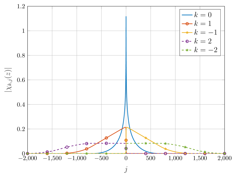
Figure 1: The perturbation coefficients for a fiber of length $2000$ km with $B=50$ GHz.

Using Rayleigh’s energy theorem and (II-B), we get the following lemma.

Lemma 5

The coefficient $\chi_{k,j}(z)$ can be found by evaluating the following integral

$$-2i\int_{k-1}^{k+1}\left(1-\lvert f-k\rvert\right)^{2}s(j,k,z,f)\,\mathit{df}$$

where

$$s(j,k,z,f)=\int_{0}^{z}\operatorname{sinc}^{2}\left((j-4\pi fz^{\prime})(1-\lvert f-k\rvert)\right)\,\mathit{dz^{\prime}}.$$ (26)

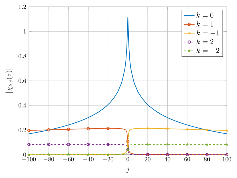
Figure 2: The perturbation coefficients for a fiber of length $2000$ km with $B=50$ GHz.

The spatial integral (26) in Lemma 5 is related to the sine integral $\operatorname{Si}(x)$ defined as

$$\operatorname{Si}(x)=\int_{0}^{x}\frac{\sin t}{t}\,\mathit{dt},$$

which can be efficiently calculated using a Padé approximation [12] or other rational approximations [13]. Using the definition of the sine integral, one can easily verify that

$$\int\operatorname{sinc}^{2}(x)\,\mathit{dx}=\frac{\operatorname{Si}(2\pi x)}{\pi}-x\operatorname{sinc}^{2}(x).$$ (27)

As a result, we have

$$\int\operatorname{sinc}^{2}(ax+b)\,\mathit{dx}= \frac{\operatorname{Si}(2\pi(ax+b))}{a\pi}$$

$$-\frac{(ax+b)}{a}\operatorname{sinc}^{2}(ax+b).$$

By choosing

$$a=-4\pi f(1-\lvert f-k\rvert),\quad b=j(1-\lvert f-k\rvert),\quad x=z^{\prime},$$

we find the antiderivative needed to evaluate the spatial integral of Lemma 5. The absolute value of $\chi_{k,j}(z)$ for a fiber of length $2000$ km is shown in Fig. 1 and Fig. 2. The channel spacing is $B=50$ GHz. In particular, Fig. 2 verifies that, as long as $j$ is not close to zero, the XPM coefficients are indeed slowly varying functions of $j$.

III Constant-Composition Codes

For any positive integer $n$, the set of all possible $n$-tuples drawn from any nonempty $m$-ary alphabet $A=\{a_{1},a_{2},\dots,a_{m}\}$ is denoted as $A^{n}$. An $n$-permutation is any invertible function mapping $\{1,\ldots,n\}$ to itself. The set of all $n$-permutations forms a group under composition called the symmetric group $S_{n}$. The $n$-permutations act on $n$-tuples over $A$ by a permutation of coordinates, so that for any $p\in S_{n}$ and any $u=(u_{1},\ldots,u_{n})\in A^{n}$, $p\cdot u=(u_{p(1)},\ldots,u_{p(n)})$.

A code $C$ of length $n$ over $A$ is any nonempty subset of $A^{n}$. The elements of $C$ are called codewords. The rate, $R$, of a code $C$ is defined as

$$R\coloneqq\frac{\log_{2}\lvert C\rvert}{n}\quad\left[\frac{\text{bit}}{\text{symbol}}\right].$$

A code $C$ is called a constant-composition code if every codeword in $C$ is a permutation of some fixed word $u\in A^{n}$. More precisely, we have the following definition.

Definition 1

A constant-composition code $C$ of length $n$ over an alphabet $A$ is a nonempty subset of $A^{n}$ such that for some $u\in A^{n}$ and for some $P\subset S_{n}$,

$$C=\{p\cdot u:p\in P\}.$$

Such a code is denoted as a $(u,P)$ CC code.

In this paper we consider only the special case where $P=S_{n}$. Associated with each $n$-tuple $v=(v_{1},v_{2},\dots,v_{n})\in A^{n}$ over the $m$-ary alphabet $A$ is an $m$-tuple called a type which counts the number of times each element of $A$ occurs as a coordinate of $v$. In particular

$$\mathrm{type}(v)=\left(w_{1}(v),w_{2}(v),\dots,w_{m}(v)\right),$$

where

$$w_{k}(v)=\sum_{j=1}^{n}\mathbbm{1}\left\{v_{j}=a_{k}\right\},\quad k=1,2,\dots,m.$$

The rate of the $(v,S_{n})$ CC code as defined in Definition 1 is then

$$R=\frac{1}{n}\log_{2}\frac{n!}{w_{1}(v)!w_{2}(v)!\cdots w_{m}(v)!},$$

where the argument of the logarithm is the multinomial coefficient that gives the number of distinct permutations of $v$. In the rest of this paper, we focus on CC codes with

$$w_{1}=w_{2}=\dots=w_{m}=1$$

so that $m=n$ and

$$R=\frac{1}{m}\log_{2}m!\approx\log_{2}\frac{m}{e}.$$

The alphabet $A$ that we consider is a subset of the complex numbers $\mathbb{C}$. We will compare performance of such CC codes with a transmission scheme where the symbols are selected independently and uniformly at random from a quadrature amplitude modulation (QAM) constellation. If the size of the constellation is $m$, the transmission rate for an independent and uniformly distributed (IUD) selection of points is

$$R=\log_{2}m\quad\left[\frac{\text{bit}}{\text{symbol}}\right].$$

The rate of a CC code of length $m$ is compared with the transmission rate of an IUD transmission scheme with a constellation of size $m$ in Fig. 3. Notice that the gap between the two curves converges to

$$\log_{2}e\approx 1.44.$$

Example 1

When transmitting IUD from a QAM constellation, an alphabet of size $64$ gives a transmission rate of $6$ bits per symbol, while to get the same transmission rate using a CC code, an alphabet size of $171$ is needed.

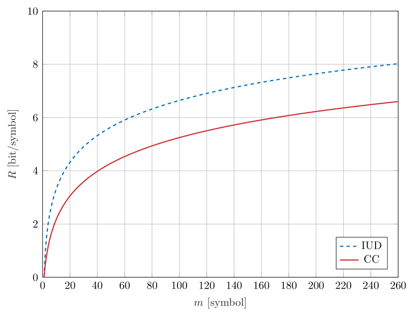
Figure 3: Transmission rate of CC codes and IUD transmission.

IV Cross-Phase Modulation Induced by Constant-Composition Codes

In this section, we consider a WDM system in which all channels use a CC code of length $m$. We assume that the symbols of each codeword are transmitted consecutively. If the $l^{\text{th}}$ codeword for transmission over channel $k$ is

$$(a_{k,lm},a_{k,lm+1},a_{k,lm+2},\dots,a_{k,lm+m-1}),$$

the symbols that we send on channel $k$ from time $j=lm$ to time $j=lm+m-1$ are

$$a_{k,lm},a_{k,lm+1},a_{k,lm+2},\dots,a_{k,lm+m-1}.$$

As shown in Section II-B, the coefficients $\chi_{k,j}(z)$ are slowly varying with $j$. For example, for the parameters used in Fig. 1 we have $\chi_{k,j}\approx\chi_{k,h}$ if

$$\lvert j\rvert>10,\quad\lvert h\rvert>10$$

and

$$\lvert j-h\rvert$$

is not too large. As long as the blocklength $m$ of the CC code used by all channels is small enough so that the above approximation is justified, the XPM term in (25) can be written as

$$\Delta_{\text{XPM}}\approx 2a_{0,0}\sum_{k\neq 0}\sum_{j=-m}^{m-1}\lvert a_{k,j}\rvert^{2}\chi_{k,j}(z)$$ (28)

$$+2a_{0,0}\sum_{k\neq 0}\sum_{l=1}^{\infty}\chi_{k,lm}(z)\sum_{j=0}^{m-1}\lvert a_{k,lm+j}\rvert^{2}$$

$$+2a_{0,0}\sum_{k\neq 0}\sum_{l=-\infty}^{-2}\chi_{k,lm}(z)\sum_{j=0}^{m-1}\lvert a_{k,lm+j}\rvert^{2}.$$

If we denote the energy of each of the codewords in the CC code used by $E$, the XPM term becomes

$$\Delta_{\text{XPM}}\approx 2a_{0,0}\sum_{k\neq 0}\sum_{j=-m}^{m-1}\lvert a_{k,j}\rvert^{2}\chi_{k,j}(z)$$ (29)

$$+2a_{0,0}E\sum_{k\neq 0}\sum_{l=1}^{\infty}\chi_{k,lm}(z)$$

$$+2a_{0,0}E\sum_{k\neq 0}\sum_{l=-\infty}^{-2}\chi_{k,lm}(z).$$

Notice that the second and the third summations in (29) are deterministic. In other words, the most important XPM terms are those that capture the nonlinear interaction of the symbol of interest with the symbols in the neighboring channels that are closest in time to the symbol of interest at the beginning of the fiber. This observation tells us that, as long as the blocklength of the CC code is not too large, the effect of most of the XPM terms in (25) is deterministic. The XPM uncertainty, therefore, will be limited to the collision of the symbols that are transmitted almost concurrently. Because of this limited XPM uncertainty, the overall observed SNR will be higher than the case of IUD symbol selection.

Remark 1

In the above explanation, the only property of the CC codes that we have used is the fact that CC codes are constant energy codes, i.e., all codewords of a CC code have the same energy. As a result, we would expect the same kind of SNR gains from more general constant energy codes. Constant energy codes are usually known as spherical codes. While we do not intend to study the performance of spherical codes in this paper, it would be interesting to see if such codes can provide performance gains. This is especially important as spherical codes can provide the same rates as CC codes with shorter blocklengths.

While CC codes are expected to reduce the uncertainty of XPM, we may at the same time observe from our model that in general the XPM term induced in detection of $a_{0,j}$ and $a_{0,h}$ is almost the same, provided that $\lvert j-h\rvert$ is not too large. In other words, we expect the effect of XPM on nearby symbols to be nearly the same. This observation, together with the fact that XPM mostly affects the phase of the detected symbols, suggest that most of the XPM induced nonlinear interference may be undone by use of phase-tracking algorithms as used in carrier recovery. Furthermore, this should be true even if IUD selection of symbols is being used.

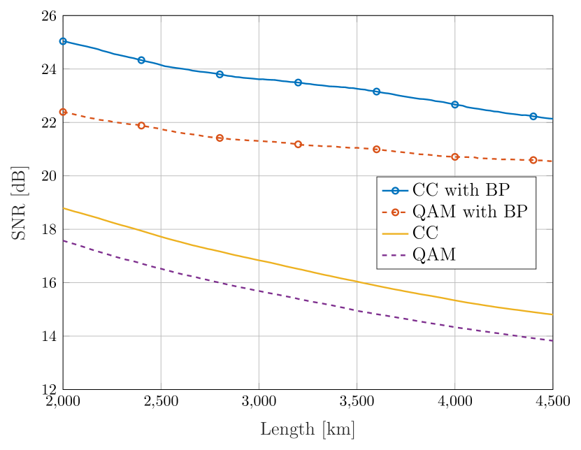
Figure 4: SNR for a CC code of blocklength $171$ and IUD transmission using $64$-QAM versus fiber length, in an idealized scenario where there is no attenuation and no amplification noise, so that the nonlinear interference noise is the only source of distortion. Two different detection schemes are considered: back-propagation (BP) followed by matched-filtering and matched-filtering without back-propagation.

In the rest of this section, we verify these two observations by trying to isolate the XPM noise in simulating data transmission using the split-step Fourier method in two scenarios: with and without carrier recovery.

IV-A Experiments without Carrier Recovery

To isolate the nonlinear interference, we consider simulating a WDM system using the split-step Fourier method with adaptive step sizes [14] in an idealized setting. The fiber is assumed to be lossless and there is no amplification noise, thus allowing us to isolate and measure interference noise. Pulses are ideal $\operatorname{sinc}(\cdot)$ functions. We assume that five WDM channels travel along the fiber without any adds and drops. The channel spacing is $50$ GHz. No guard band is assumed.

Two types of detection are considered. The first one consists of detection using a matched filter as explained in Section II-B. In the second detection method, the channel of interest is fully back-propagated after being selection by a low-pass filter at the receiver. This is then followed by matched filtering and sampling. Phase compensation is done by a common phase rotation applied to all symbols chosen so that the average residual phase of the whole sequence of symbols is $0$.

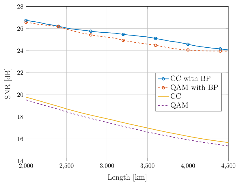
Figure 5: SNR for a CC code of blocklength $171$ and IUD transmission using $64$-QAM versus fiber length, in an idealized scenario where there is no attenuation and no amplification noise, so that the nonlinear interference noise is the only source of distortion. Two different detection schemes are considered: back-propagation (BP) followed by matched-filtering and matched-filtering without back-propagation. The samples of the matched filter are back-rotated by using a genie-aided blind phase search algorithm.

The resulting channel is modelled as an additive noise channel

$$Y=X+N$$

where $X$ is the input random variable, $Y$ is the output random variable, and $N$ is the additive noise (caused by interference) for which, SNR is defined by

$$\text{SNR }=\frac{\mathbb{E}[\lvert X\rvert^{2}]}{\mathbb{E}[\lvert N\rvert^{2}]}$$

and is approximated by numerical averaging in place of statistical expectations. The transmission length has been varied from $2000$ km to $4500$ km in steps of $20$ km. An IUD transmission with a square $64$-QAM, as well as a CC code of blocklength $171$ are considered. The alphabet used for the CC code is not optimized in any sense and is selected simply by picking $171$ points of a $256$-QAM constellation having the least energy.

The results are shown in Fig. 4. The results show that CC codes provide a gain of about $1$ dB over IUD QAM without back-propagation, and they provide a gain of about $2$ dB with back-propagation at the receiver. Thus CC codes are indeed effective in reducing the uncertainty due to XPM in the received signal.

IV-B Experiments with Carrier Recovery

Under the same setup, a different decoder that incorporates a blind phase search (BPS) algorithm [15] at the very last step to minimize the phase error is considered. The decoder used is a genie-aided one as it uses the transmitted symbols to perform the best phase compensation that one might expect from the blind phase search algorithm. When detecting the symbol of interest $X_{0}=a_{0,0}$, the BPS is done by solving the following minimization problem:

$$\phi_{0}=\operatorname*{arg\,min}_{\theta}\sum_{j=-N}^{N}\lvert X_{j}-Y_{j}e^{i\theta}\rvert^{2},$$ (30)

in which $X_{j}$ is the $j^{\text{th}}$ transmitted symbol and $Y_{j}$ is the corresponding output of the matched filter. The output of the matched filter is rotated by $\phi_{0}$ and the output of the BPS block is $Y_{0}e^{i\phi_{0}}$. The window size of the BPS block is set to $2N+1=21$.

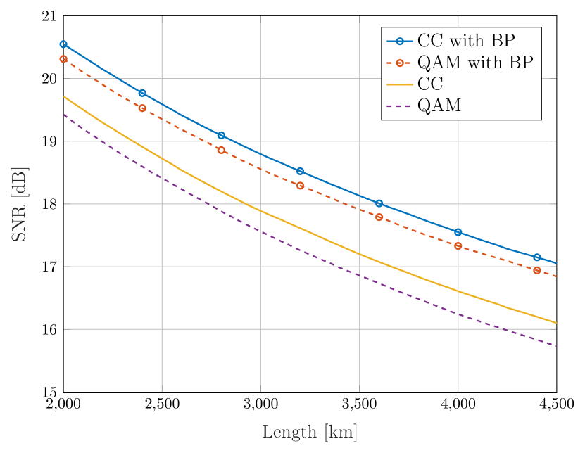
Figure 6: SNR for a CC code of blocklength $171$ and IUD transmission using $64$-QAM versus fiber length. Two different detection schemes are considered: back-propagation (BP) followed by matched-filtering and matched-filtering without back-propagation.

The SNRs are shown in Fig. 5. As expected, the SNR gain of the CC code is considerably smaller when using BPS. The SNR gain without back-propagation is reduced to $0.2$ to $0.5$ dB, while the SNR gain with back-propagation is between $0$ to $0.5$ dB, depending on the length.

IV-C More Realistic Experiments

To properly simulate single-polarized data transmission over the optical fiber, we take into account the attenuation of the fiber. It is assumed that an erbium-doped fiber amplifier (EDFA) is located at the end of each span of length $50$ km. Pulse shaping is done by using a root-raised cosine pulse with a roll-off factor of about $6$%. The channel spacing is $50$ GHz including about $6$% guard band. Among the five WDM channels considered, the channel of interest, as before, is the middle one. The SNRs obtained for the CC code of blocklength $171$ as well as the IUD transmission from a $64$-QAM constellation are shown in Fig. 6 when no carrier recovery is in place. The results of detection with BPS are shown in Fig. 7. The SNR gain of CC codes in the absence of BPS is about $0.3$ dB without back-propagation and about $0.2$ dB with back-propagation. With BPS, however, the SNR gain of CC codes is negligible (about $0.05$ dB).

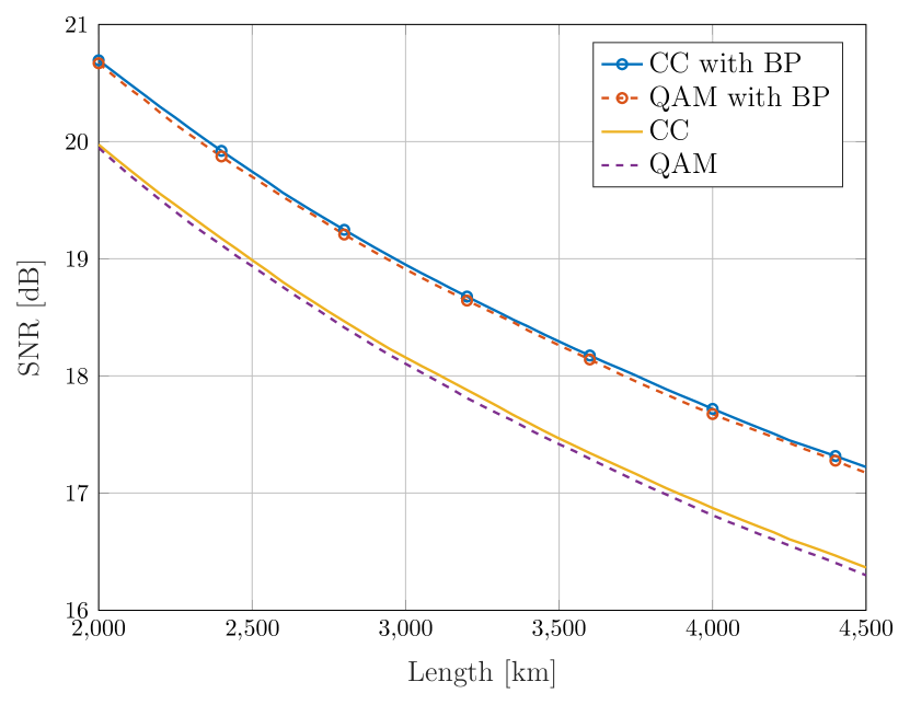
Figure 7: SNR for a CC code of blocklength $171$ and IUD transmission using $64$-QAM versus fiber. Two different detection schemes are considered: back-propagation (BP) followed by matched-filtering and matched-filtering without back-propagation. The samples of the matched filter are back-rotated by using a genie-aided blind phase search algorithm.

V Conclusions

Using a first order perturbation model derived from the nonlinear Schrödinger equation, we have shown why short constant-composition codes reduce nonlinear interference noise in a WDM system. We have also shown that phase tracking can be used to achieve the same reduction in nonlinear interference noise even without using constant-composition codes.

Our analysis shows that the more general class of spherical codes, which encompass constant-composition codes, have the potential to reduce cross-phase modulation, as long as their blocklength is not too long. We leave the investigation of the potential gains provided by spherical codes as future work.

References

- [1] R.-J. Essiambre, G. Kramer, P. J. Winzer, G. J. Foschini, and B. Goebel, “Capacity limits of optical fiber networks,” J. Lightw. Techn., vol. 28, no. 4, pp. 662–701, Feb. 2010.
- [2] A. Mecozzi and R.-J. Essiambre, “Nonlinear Shannon limit in pseudolinear coherent systems,” J. Lightw. Techn., vol. 30, no. 12, pp. 2011–2024, Jun. 2012.
- [3] R. Dar and P. J. Winzer, “Nonlinear interference mitigation: Methods and potential gain,” J. Lightw. Techn., vol. 35, no. 4, pp. 903–930, Feb. 2017.
- [4] A. Amari, S. Goossens, Y. C. Gültekin, O. Vassilieva, I. Kim, T. Ikeuchi, C. M. Okonkwo, F. M. J. Willems, and A. Alvarado, “Introducing enumerative sphere shaping for optical communication systems with short blocklengths,” J. Lightw. Techn., vol. 37, no. 23, pp. 5926–5936, Dec. 2019.
- [5] T. Fehenberger, H. Griesser, and J.-P. Elbers, “Mitigating fiber nonlinearities by short-length probabilistic shaping,” in Optical Fiber Commun. Conf. OSA, 2020, p. Th1I.2.
- [6] T. Fehenberger, D. S. Millar, T. Koike-Akino, K. Kojima, K. Parsons, and H. Griesser, “Analysis of nonlinear fiber interactions for finite-length constant-composition sequences,” J. Lightw. Techn., vol. 38, no. 2, pp. 457–465, Jan. 2020.
- [7] W.-R. Peng, A. Li, Q. Guo, Y. Cui, and Y. Bai, “Baud rate and shaping blocklength effects on the nonlinear performance of super-symbol transmission,” Optics Exp., vol. 29, no. 2, pp. 1977–1990, Jan. 2021.
- [8] K. Wu, G. Liga, A. Sheikh, F. M. J. Willems, and A. Alvarado, “Temporal energy analysis of symbol sequences for fiber nonlinear interference modelling via energy dispersion index,” J. Lightw. Techn., vol. 39, no. 18, pp. 5766–5782, Sep. 2021.
- [9] L. K. Wickham, R.-J. Essiambre, A. H. Gnauck, P. J. Winzer, and A. R. Chraplyvy, “Bit pattern length dependence of intrachannel nonlinearities in pseudolinear transmission,” IEEE Photonics Techn. Lett., vol. 16, no. 6, pp. 1591–1593, Jun. 2004.
- [10] S. Civelli, E. Forestieri, and M. Secondini, “Interplay of probabilistic shaping and carrier phase recovery for nonlinearity mitigation,” in Europ. Conf. Opt. Comm. IEEE, 2020, pp. 1–4.
- [11] G. Agrawal, Nonlinear Fiber Optics, 5th ed. Elsevier Academic Press, 2017.
- [12] B. T. Rowe, M. Jarvis, R. Mandelbaum, G. M. Bernstein, J. Bosch, M. Simet, J. E. Meyers, T. Kacprzak, R. Nakajima, J. Zuntz et al., “GALSIM: The modular galaxy image simulation toolkit,” Astronomy and Computing, vol. 10, pp. 121–150, Apr. 2015.
- [13] A. J. MacLeod, “Rational approximations, software and test methods for sine and cosine integrals,” Numerical Algorithms, vol. 12, no. 2, pp. 259–272, Sep. 1996.
- [14] O. V. Sinkin, R. Holzlohner, J. Zweck, and C. R. Menyuk, “Optimization of the split-step Fourier method in modeling optical-fiber communications systems,” J. Lightw. Techn., vol. 21, no. 1, pp. 61–68, 2003.
- [15] T. Pfau, S. Hoffmann, and R. Noé, “Hardware-efficient coherent digital receiver concept with feedforward carrier recovery for -QAM constellations,” J. Lightw. Techn., vol. 27, no. 8, pp. 989–999, 2009.