Machine Learning Simulates Agent-Based Model Towards Policy

Abstract

Public Policies are not intrinsically positive or negative. Rather, policies provide varying levels of effects across different recipients. Methodologically, computational modeling enables the application of multiple influences on empirical data, thus allowing for heterogeneous response to policies. We use a random forest machine learning algorithm to emulate an agent-based model (ABM) and evaluate competing policies across 46 Metropolitan Regions (MRs) in Brazil. In doing so, we use input parameters and output indicators of 11,076 actual simulation runs and one million emulated runs. As a result, we obtain the optimal (and non-optimal) performance of each region over the policies. Optimum is defined as a combination of GDP production and the Gini coefficient inequality indicator for the full ensemble of Metropolitan Regions. Results suggest that MRs already have embedded structures that favor optimal or non-optimal results, but they also illustrate which policy is more beneficial to each place. In addition to providing MR-specific policies’ results, the use of machine learning to simulate an ABM reduces the computational burden, whereas allowing for a much larger variation among model parameters. The coherence of results within the context of larger uncertainty–vis-à-vis those of the original ABM–reinforces robustness of the model. At the same time the exercise indicates which parameters should policymakers intervene on, in order to work towards precise policy optimal instruments.

JEL Classification]C63, H71, R38

1 Computational Models for Policy

Policymakers know that policies, as broad as they may be, lead to different results in different contexts stone_understanding_2017 ; Mitchell.Woodman2010Regulationandsustainableenergysystems ; Gawel.etal2016Supportpoliciesforrenewablesinstrumentchoiceandinstrumentchangefromapublicchoiceperspective . Why certain policies impact different regions differently, however, is difficult to pinpoint cravo_economic_2013 ; Boschma2013ConstructingRegionalAdvantageandSmartSpecializationComparisonofTwoEuropeanPolicyConcepts ; Lundvall2007NationalInnovationSystemsAnalyticalConceptandDevelopmentTool . Interest groups, institutions and context may be relevant factors for how policies are elaborated, implemented, revised and assessed mueller_why_2020 ; Nelson1994Thecoevolutionoftechnologyindustrialstructureandsupportinginstitutions ; Hochstetler.Kostka2015WindandSolarPowerinBrazilandChinaInterestsStateBusinessRelationsandPolicyOutcomes . In that sense, existing structural factors, such as households attributes, income and location, along with characteristics of businesses and government might play a role Faber.etal2010ExploringdomesticmicrocogenerationintheNetherlandsAnagentbaseddemandmodelfortechnologydiffusion .

Computational models may act as a coherent set of sequential rules and procedures that help understand, explore, and learn about effects and impacts of policies Tesfatsion2011AgentbasedModelingandInstitutionalDesign . Models allow for the anticipation of possible results doi:10.1098/rsos.172096 ; deMarchi.Page2014AgentBasedModels ; Faber.etal2010ExploringdomesticmicrocogenerationintheNetherlandsAnagentbaseddemandmodelfortechnologydiffusion . Additionally, computational models make counterfactual tests not only feasible, but a must when making decisions on policies Lamperti.etal2018FarawaySoCloseCoupledClimateandEconomicDynamicsinanAgentbasedIntegratedAssessmentModel ; Lespagnol.Rouchier2018TradingVolumeandPriceDistortionAnAgentBasedModelwithHeterogenousKnowledgeofFundamentals ; Huang.etal2010Financialcrisesandinteractingheterogeneousagents . Policymakers facing complex scenarios would be in a better position to make decisions when they have subsidies from an array of factual and counterfactual indicatorsBrenner.Werker2009Policyadvicederivedfromsimulationmodels ; Schmidt.etal2016DodeploymentpoliciespicktechnologiesbynotpickingapplicationsAsimulationofinvestmentdecisionsintechnologieswithmultipleapplications .

Agent-based models (ABMs) fit a class of computational models in which the emphasis lies on the agents of a system, the minimum decision-making units, and their interactions Tesfatsion2003Agentbasedcomputationaleconomicsmodelingeconomiesascomplexadaptivesystems ; Arthur2006OutofEquilibriumEconomicsandAgentBasedModeling . It is a bottom-up approach in which agents follow deterministic rules and interact to reproduce known patterns Axelrod1997Thecomplexityofcooperationagentbasedmodelsofcompetitionandcollaboration ; Janssen.Ostrom2006Empiricallybasedagentbasedmodels . Moreover, ABMs are discrete, dynamic systems in which agents of various kind and their environment co-evolve following algorithmic steps epstein_growing_1996 ; Vazquez.Hallack2018TheroleofregulatorylearninginenergytransitionThecaseofsolarPVinBrazil . ABMs are tools that social scientists, in particular, may use to systematically codify tacit knowledge and behaviors and ”animate” trajectories in order to experiment galan_errors_2009 ; Chen.etal2001Testingfornonlinearstructureinanartificialfinancialmarket ; Ehrentreich2008TheOriginalSantaFeInstituteArtificialStockMarket .

Specifically, PolicySpace2 (PS2) is an spatial-economic agent-based model that uses census and geographical data for households, businesses and municipalities within Metropolitan Regions (MRs) to simulate interactions in the housing, labor, goods and services markets. The empirical, intraurban model runs from 2010 to 2020 and is used to simulate three policy tests. Validation is made to Brasilia, the capital of Brazil, and additional results are also presented to four other MRs alves_furtado2022 .

We use PolicySpace2 (PS2) open source as our simulation baseline model for this paper. However, whereas PS2 ran manual–hundreds–combinations of parameters for its sensitivity analysis, we design a surrogate model that expands the analyses to one million possible combinations.

A surrogate model is a computational artifice that simultaneously mimics the procedures of a model using its inputs and outputs, whereas saving time and maximizing outputs. ”An emulator is thus a model of a model: a statistical model of the simulator, which is itself a mechanistic model of the world” (paleyes_emulation_2019, , p.2). Surrogate models provide a simple and cheap option to emulate the original run of a model to a higher order of magnitude vanderHoog2019SurrogateModellinginandofAgentBasedModelsAProspectus ; tenBroeke.etal2021TheUseofSurrogateModelstoAnalyseAgentBasedModels .

Given this context, our research question is twofold. First, we want to learn whether different policies generate optimal results in different Metropolitan Regions? Or do they always influence the same? In other words, we would like to know whether each policy affects the different MRs heterogeneously or if there is one-size-fits-all policy for all places. Secondly, we wonder whether there are model parameters and rules that would have higher (or lower) values associated to optimal scenarios. Thus, which parameters and rules would demand (if possible) policymakers intervention in order to nudge their MRs towards optimal scenarios?

In order to answer these questions we applied Machine Learning (ML) procedures to create a surrogate model that emulated an Agent-Based Model, PolicySpace2, and explored results of three alternative policies against the no-policy baseline for an array of 46 Brazilian MRs. As such, we anticipated empirical scenarios for each policy and each MR and contrasted these results with the absence of policy. Results expanded the test originally made by the ABM–which implied a quasi-manual test of 11 thousand runs on mostly five MRs–and amplified the combination of parameters values to one million runs.

We chose a relational, comparative optimum ex-post target for our policy analysis. Basically, the optimal status results simultaneously imply that the Metropolitan Region has achieved the highest quartile of GDP and the lowest quartile of Gini coefficient. This choice was made to train the ML and execute the expansion of runs into a larger scope that included all parameters and MRs. Hence, optimal in this case refers to GDP and Gini coefficient indicators comparatively to all other MRs.

The contribution of the paper is to expand the empirical results of a policy-test ABM while bringing more uncertainty and more robustness to the simulation process. More uncertainty as we emulated the ABM with a much larger set of combinations among parameters that enter the model, compared to the original ABM run. More robustness as we explored results over one million outputs instead of the original 11,076 simulation runs.

Additionally, we produced a rank of Metropolitan Regions intrinsic attributes that measures their response to an specific pair of optimal policy indicator targets and policy proposal. The response also illuminated the best policy for each individual MR. Finally, we presented a surrogate model that qualify as a valid approach for spatial ABM generalization.

2 Literature background

In this section we discuss the pertinent literature background. First we briefly review the literature on ABM and their use for policy analysis. Then we review the literature on ML and then intersection with ABM: surrogate models.

ABMs are simulation models that highlight interactions between decision-making units, the agents, and their local environment. ABMs basically consist of a discrete system in which the states of the agents and the environment are updated according to explicit rules epstein_growing_1996 .

Policy analysis specifically seem to be a perfect use of ABMs. First, public policies constitute complex systems with a number of ever-changing agents (citizens, politicians, businessmen, scientists, institutions) acting and reacting in time and space, with limited information, and unaware of others rationality furtado_modeling_2015 ; geyer_handbook_2015 ; arthur_inductive_1994 .

Secondly, ABMs do not need to work with a single–likely to fail mueller_why_2020 –policy goal. Quite on the contrary, ABMs are fit to work as a communication tool gilbert_computational_2018 that makes the analysis systemic and visual, enabling parties from different backgrounds, experiences and disciplines to converse and exchange, whilst producing probabilistic scenarios.

Thirdly, computational modeling in general and ABMs in particular are suitable for experimenting. Counterfactuals and what-if questions are formulated and tested within a safe environment, with costs restricted to the computational burden, and the time-consumed from modelers, programmers and policymakers.

There has been a plethora of models using ABMs in a variety of disciplines, methods and applications edmonds_simulating_2017 ; lee_complexities_2015 ; heppenstall_agent-based_2012 ; dawid_agent-based_2018 ; adepetu_agent-based_2016 ; scott_simdrink:_2016 ; ingham-dempster_tim_agent-based_2017 ; van_der_veen_exploring_2017 . However, a much smaller number has been actually applied and used to aid and change real policy carley_biowar_2006 ; kerr_covasim_2021 ; gilbert_computational_2018 . Mainly, the difficulty comes from the hurdle of bridging ”the gap between policy practice, often expressed in qualitative and narrative terms, and the scientific realm of formal models” (ahrweiler_modelling_2015, , p.1). Nevertheless, ABMs have proved to be valuable policy tools gilbert_computational_2018 , when observing its limitations aodha_pitfalls_2017 .

In this paper, we focus mainly on the expansion of the original model’s capacity to anticipate policy trajectories and thus enable policy decision-making. Hence, the analysis supports comparison and evaluation of alternative policies, or rather, alternative decisions on public money investing, before actually spending taxpayers’ money.

2.1 Machine learning and surrogate models

ML consists of a series of computer methods in different areas within mathematics and statistics that attempt to automate the processes of finding, sorting and weighting different patterns in data sets. Moreover, ML aims at finding ”hidden rules” in order to predict and analyze data Breiman2001Randomforests . This is a relevant characteristic that differentiates ML from statistics or econometrics: organizing data from various sources with an emphasis on predicting and forecasting.

ML is typically divided between supervised and unsupervised learning. Supervised learning has an optimal, target or desired output for its models. Unsupervised learning has no target and identifying patterns or clustering is the main goal. In this paper, we apply a supervised learning process in which the target is an inter-city comparative optimal duet of indicators (see subsection Methods: Procedures).

Machine Learning also include semi-supervised and reinforcement learning. In semi-supervised ML, some data contain labels–whereas the complementing data do not–, and it is mostly used for classification. In fact, information on the labeled data may be used to inform the unlabeled ones van_engelen_survey_2020 . Reinforcement learning focuses on a reward function that guides the learning process of agents.

Random forest is a common method within supervised ML. A random forest consists of a selection of subsets that branch randomly into different trees. Those subsets are independent and non-identical decision trees defined by independent random vector parameters and input data. With a large number of trees, the algorithm then searches for the most popular class through equal-weight voting Breiman2001Randomforests ; Ren.etal2017Researchonmachinelearningframeworkbasedonrandomforestalgorithm ; Mishina.etal2015BoostedRandomForest .

In this paper we tested different ML methods and chose a random forest surrogate model that emulates the original simulation model, PS2 alves_furtado2022 . ”A surrogate model is an approximation method that mimics the behavior of an expensive computation or process. (…) [a surrogate model] can be trained to represent the system, learning a mapping from simulator inputs to outputs” (lavin_simulation_2021, , p.11). Moreover, surrogates are essentially emulators that substitute an actual simulation model for a simpler method in order to produce results through less demanding means, both in relation to time and to processing power. Through the use of ML, it reiterates over the ABM using pre-processed input and output information.

A surrogate model has advantages that seem to be adequate for our proposed exercise:

1. Generalization. A surrogate enables many more combinations of input parameters. In practice, the surrogate model works as if we had run the original simulation model a much higher number of times, whilst testing a (much) wider range of possible parameters.

2. Practicality and speed. Running a surrogate 1,000,000 times is way faster (and actually feasible) than running 1,000 regular simulations. It is a different order of magnitude concept. The simulations are emulated, rather than actually run. This is especially valid for models with geographical information and a large number of agents.

3. Statistical extrapolation. Surrogate models’ larger number of runs bring statistical relevance for the results and provides robustness for the extrapolation.

The aim of our surrogate is to extract the most information of the model with as little computational time as possible, choosing an optimal target while doing so. We revise surrogate models in relation to the three main steps in producing a surrogate.

In the ML surrogate proposed by Lamperti.etal2018Agentbasedmodelcalibrationusingmachinelearningsurrogates , the authors explore the parameter space through the use of a non-parametric ML surrogate without prior knowledge of the spatial distribution of data. Starting with a sample of initial conditions values (through Sobol sampling), random subsets are drawn, ran through the ABM and then evaluated by user-defined criterion of positive or negative. Then the surrogate is learned through a ML algorithm using a variation of random forest. By repeating the steps, the surrogate predicts the probability of false negatives (non-optimal results that are actually optimal) and is developed focusing on producing less false negatives. In a nutshell, the ABM is ran each time, it processes the data, labels and evaluates the results.

The surrogate of Lamperti.etal2018Agentbasedmodelcalibrationusingmachinelearningsurrogates is directly comparable to the surrogate models that use Bayesian emulation or kriging, such as the model of tenBroeke.etal2021TheUseofSurrogateModelstoAnalyseAgentBasedModels . According to the authors, their kriging surrogate is built through: model specification through a prior-distribution of hyper-parameters, then the ABM is ran and results are gathered by the use of an integration function of the generalized least squares estimator of positive-definite symmetric matrices. The modeler then must choose a simulator: a multi-output (MO) emulator or a many to single-output. The authors choose the multi-output (MO) emulator due to convenience and least computational time tenBroeke.etal2021TheUseofSurrogateModelstoAnalyseAgentBasedModels . By using the MO emulator, one may use the produced surrogate to make model predictions. Their surrogate is quite similar to that of Conti.OHagan2010Bayesianemulationofcomplexmultioutputanddynamiccomputermodels , especially in relation to the discussion of multi-output emulators versus other options. Essentially, their surrogate separates data into training and testing classifications, expanding the training data until sufficient performance (decided ad hoc by the modeler) is reached.

The surrogate of Hayashi.etal2016ImprovingBehaviorPredictionAccuracybyUsingMachineLearningforAgentBasedSimulation focuses on the parameter space of the simulation. The authors use four ML methods, with neural networks and random forests being part of those tested. The authors analyze many inputs to one output, again separating between ”positive” and ”negative” outcomes. ML feeds back the ABM by revising the inner workings of agents with each round of the simulation restarting with initial conditions given by the ML process. Their models connects the ABM and ML portions by comparing their results, attempting to minimize the error between the outputs of the ABM and the ML surrogate.

The surrogate of Edali.Yucel2019Exploringthebehaviorspaceofagentbasedsimulationmodelsusingrandomforestmetamodelsandsequentialsampling relies heavily on random forest and focuses on output predictions. For the training and fitting of the surrogate, they use the latin hypercube sampling and then sequential sampling. It combines random forests with uncertainty sampling in order to train the surrogate model.

The surrogates we reviewed interact with an ABM model or the modeler itself to increase the quality of the prediction or the performance of the original model. Our proposal is somewhat independent of the original ABM. Our surrogate uses input and output from the original ABM to learn the inner mechanisms–the mapping–that transforms inputs into outputs. Once trained, a new analysis that takes advantage of a much larger parameter space (unfeasible for the case of the original ABM) is applied with a clear target of policy optimality. The results are then compared providing a counterfactual panorama for policymakers.

In the next section, we describe first the basics of the original PS2 model, then the data generated by PS2 and used as input to our surrogate model. After that, we detail the procedures and steps that we use in running the emulator.

3 Methods

3.1 Baseline Agent-Based Model: PolicySpace2 (PS2)

PolicySpace2 (PS2) is an open source, readily available ABM that focuses on three alternative policy-schemes for the case of Brazilian MRs. According to the authors, PS2 is defined ”as a primarily endogenous computational agent-based model (ABM) that includes mortgage loans, housing construction, taxes collection and investments, with firms and households interacting in real estate, goods and services, and labor markets” (alves_furtado2022, , par.1.5). The default run of PS2 is for the MR of Brasília from 2010 to 2020, using census and business data, along with detailed geographical intraurban (census tract equivalent) boundaries.

The main goal of PS2 is to contrast and compare three competing policy investments alternatives for the case of Brasília. Given low-income households, municipalities may either (a) acquire houses to transfer (Property acquisition); (b) provide rental vouchers (Rent vouchers); or (c) make monetary transfers (Monetary aid). These policies are tested against a no-policy baseline and results are compared using macroeconomic indicators and their trajectories.

The results of PS2 consistently show that Rent vouchers (b) and Monetary aid (c) seem to be the most beneficial policy choice producing higher GDP with a lower Gini coefficient. These two options also reduced the percentage of households defaulting on rent and going any month without goods and services consumption. The policy choice of Property acquisition seems to perform worse in comparison to the two alternatives and the no-policy baseline across most of the indicators alves_furtado2022 .

PS2, however, is developed and evaluated for the case of Brasília Metropolitan Region alone. Although the authors also run the model and present comparisons to four other MRs, results were not exhaustively run for all of the 46 available MRs. This is exactly how the surrogate model we present contribute to the analysis. We use the bulk of runs of the sensitivity analysis to expand the results to all 46 MRs, while also expanding the variability contained in the data–better exploring the parameter space–,and steering results towards optimal policies.

3.2 Data

In order to emulate the original PS2 ABM, we started out with two sets of data produced in the 11,076 runs the authors of PS2 executed alves_furtado2022 . The data provided by the authors included 32 sets of sensitivity analysis on different parameters (typically with 7 interval values and 20 runs each), runs for all MRs, runs for specific MRs, and sets of 20 runs for each one of the four alternative policy instrument. For all runs, we accessed the parameters’ configuration for each one, as well as the the outputs–in terms of indicators produced by the model–associated with each configuration of parameters (see the left ABM portion of figure 1).

The configuration of parameters and rules includes information such as which Metropolitan Region is being simulated; the percentage of the total population used for a given run; the choice of wage-decision the firms used; or which policy is tested, if any. The full list of parameters include: (a) all of those in table 2, (b) the Boolean choices of table 3, and (c) each MR, as listed in table 6. Moreover, parameters include a test of tax distribution, interest rate alternatives, availability of construction lots, and simulation starting year.

Additionally, PS2 produced an array of 66 indicators, providing details that refer to municipalities of a MR, but that also contained information on households, workers, businesses, and the bank. All in all, our data mapped the exact configuration of parameters for each run to the set of indicators produced by that same run. We then proceeded to the learning process that maps inputs to outputs and enables extrapolation using the surrogate ML model.

3.2.1 Concept and design of the optimal

Here comes the ”towards policy” part of the paper. Instead of just learning patterns from data (unsupervised machine learning), we have opted to apply a supervised ML to construct a surrogate model that purposefully steers towards policy. A model that comparatively distinguishes whether the tested policies–and their associated parameters–are socially beneficial or not.

A large portion of public economic debate surpasses the growth of the economy, and adopts GDP as its main indicator. There has been some attempts to qualify the discussion and include other dimensions, such as a Human Development Index (HDI), a focus on the United Nations Sustainable Development Goals (UN-SDG) guerrero_policy_2020 ; guerrero_how_2022 , or even include happiness as a subjective indicator, although with limited reach austin_well-being_2016 .

We decided to focus simultaneously on GDP (production) and Gini coefficient (inequality) on the surrogate model. The algorithm enables the surrogate with any choice of pair of indicators available in the original model, along with their threshold quantiles. The other output indicators available included: inflation, unemployment, household consumption and wealth, infrastructure investment, GDP and Gini coefficient. Given the alternatives, we considered that the pair of indicators that conveys the stronger combination of optimal policy were the greatest GDP with the smallest Gini coefficient. As such, the economy shows strength at the same time that distributes its growth. 2022:39: Hence, the binary classification of optimal and non-optimal encompasses all simulation runs–out of the total sample of 11,076–that simultaneously qualifies along the superior quartile (.75) of GDP indicator and the inferior quartile (.25) of the Gini coefficient indicator. The quartiles were chosen to reflect a reasonable number of runs as optimal.

The optimal in this case is designed as a comparative and relational statistic among the set of 46 MRs. As such, we may say that optimal refers to a national bundle that includes larger and smaller MR with diverse historical attributes, economic prevalence, population composition, businesses development and accessibility.

The idea is that the surrogate model enables a counterfactual optimum as an would-be ex-post analysis, before actually implementing any of the policies. Given a photo of the existing attributes of each Metropolitan Region, the surrogate responds which policy–if any–would change the status quo for the better, given the national context.

3.2.2 Generation of parameters

Parameters are generated according to two processes:

• If they are discrete parameters or rules, they are chosen according to a probability that is simply the inverse of the number of alternatives ($m^{-1}$), being $m$ the number of possibilities for each dummy analyzed. In the case of policies, for example, each one of the three policies tested, along with the no-policy baseline, had a 0.25% probability.

• If they are continuous parameters, they are drawn from a truncated normal distribution, given the lower and upper bounds (see table 8), the mean, and a three times larger standard deviation from the original sample.

3.3 Procedures

The step-by-step of the implementation of the surrogate is as follows (figure 1). The code for the steps listed below is available at https://www.comses.net/codebase-release/a336c854-d89d-44a1-adbc-50ae092e64de/. Please refer to the README.md file for instructions on how to run the code:

1. The PS2 ABM was manually run by the original authors, producing 11,076 individual runs. Each run contains the configuration parameters: (a) including exogenous parameters, (b) rules and decision-making choices, (c) each one of tested policies – or the no-policy baseline, (d) the necessary initial municipal input data, and the output of the model containing all final indicators of the simulation. Examples of each one include:

   • Exogenous parameters: workers’ productivity, mortgage interests, businesses’ markup, or the relevance of neighborhood quality perception in housing prices.

   • Rules and decision-making mechanisms: whether to consider distance to the firm as a job application criteria, how to set workers’ wage, or how to distribute metropolitan funds.

   • Policies: each one of the three tested policy, plus the no-policy baseline.

   • Municipal data: local information on households composition, workers qualification, businesses, and the intraurban spatial configuration. Municipal data is constant. However, one of the parameters determines the initial year, and thus the original data, to be either 2010 (default), or 2000.

2. We then mapped the input configuration parameters to the output indicators, constructing the typical ML X matrix. Hence, every configuration of parameters is linked to the output of the simulation depicted by the indicators.

3. Next, we constructed the optimal and non-optimal from output indicators, thus producing the typical ML Y vector.

4. We proceeded to the separation of original sample between training and test sets using the typical python scikit-learn (skelarn) model selection procedure of train-test split, with test size of .25 and random state of 10. Then, we trained the model and tested it (see table 1).

5. Afterwards, we generated 1,000,000 new parameters, expanding the original configuration parameters into one million combinations (see subsection Methods: Generation of parameters).

6. We applied the learning algorithm. Running of the ML random forest itself (see subsection Methods: ML implementation).

7. Then, we applied the learned ML algorithm to the newly generated parameters to find optimal or non-optimal results.

8. Finally, we analyzed the results.

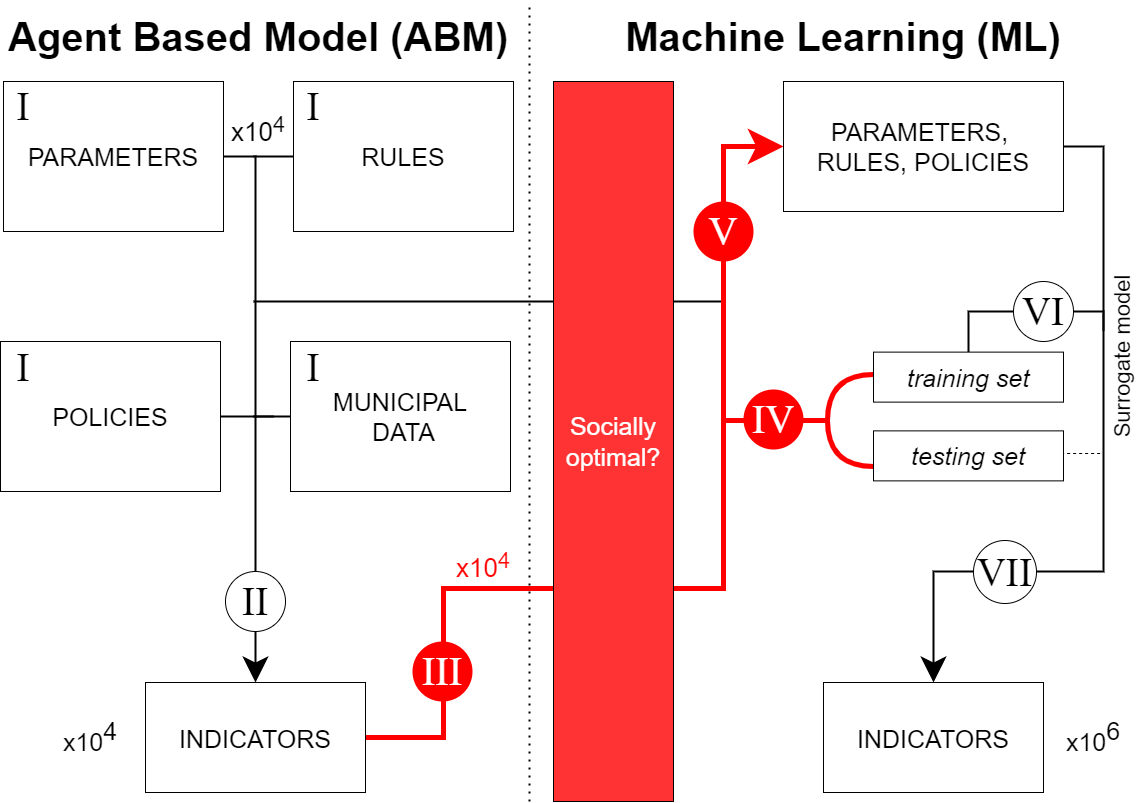
Figure 1: The figure depicts the steps taken to emulate the original ABM, whilst amplifying the possible combination of parameters and steering the results towards optimal policy. The original ABM (left side) produced sample configuration parameters and output indicators (I and II). Indicators were then divided between optimal and non-optimal depending on their relative GDP and Gini coefficient indicators (III). A set of 1,000,000 new parameters were generated and trained in the ML surrogate model, producing one million results (IV–VIII).

In a nutshell, the ABM and the ML surrogate model are separated in their inner-workings. First, the ABM itself runs and produces outputs from configuration parameters, with some variation. Secondly, the output indicators enable the optimal classification. Finally, a much larger configuration of parameters uses the learned ML model–the surrogate–to generate new outputs.

We implemented and tested some ML implementations, such as support-vector machine (SVC), Multi-layer Perceptron Classifier (MLPC) and a Voting Classifier. The SVC and MLPC were unable to predict optimal cases. See from table 4 in the appendix that their optimal predictions were observed to be in fact non-optimal. These two unadjusted results influenced the Voting Classifier, which is a weighted score of the models tested.

Hence, we chose the Random Forest Classifier method that was able to correctly predict optimal and non-optimal cases. We applied the Random Forest using $10^{4}$ trees, Gini criterion, with a maximum depth of 15 for each tree. The confusion matrix is presented at table 1. The results obtained led to an accuracy of 0.9917 with a precision of 0.9863. However, the recall was not so good at 0.8727, with an F1 indicator of 0.9260. Considering that these results were obtained after 11,076 time-consuming simulation runs, we understand that the surrogate is adequate for the exercise proposed.

The simulation run of the baseline model takes about 30 minutes in the standard server of our institution. The default configuration also allows for simultaneous runs on different cores, which enables 20 runs in the same 30 minutes. Even if we had 100 cores and ran 100 simulations at the same time, we would still need 300,000 minutes, or 5,000 hours, which represents more than 208 days. The surrogate equivalent runs in less than 2–3 hours.

We tried to avoid errors and artefacts in the sense proposed by galan_errors_2009 . alves_furtado2022 claim to have made extensive sensitivity analysis of parameters and rules, along with multiple simulations, and also makes the code and documentation open. Our results reinforce the robustness of the ABM output, with a wider parameter space. The application of the ML surrogate is straightforward and uses typical python/scikit-learn implementation. Nevertheless, we provide the code and data. Please refer to the README.md file for instructions on how to run the code: https://www.comses.net/codebase-release/a336c854-d89d-44a1-adbc-50ae092e64de/.

Table 1: Confusion matrix for the random forest ML implementation. The random forest was the model with best accuracy–0.9917–predicting only 2 optimal cases which were actually non-optimal, whereas 21 cases that were actually optimal were predicted to be non-optimal.

		Predicted
		Non-optimal	Optimal
Observed	Non-optimal	2602	2
	Optimal	21	144

4 Results and Discussion

In this section, we first present the results of the cities classification across each of the competing policies. Then, we detail the difference in parameters and rules given by the optimal and non-optimal classification.

4.1 Metropolitan Regions results per policy

Figure 2 shows the performance of all MRs for each policy in terms of percentage of optimal runs, given the optimum definition of best quartile of GDP and lowest quartile of Gini coefficient. On average (see table 5), 17.87% of the simulations performed optimally for the no-policy baseline. Three MRs performed relatively better than the others (Belo Horizonte, São Paulo and Rio de Janeiro), whereas four others performed worse (Belém, Porto Alegre, Campinas and Brasília). All of the remaining 39–most with smaller total population (see table 9)–were classified as optimal between 19% and 12% of their own runs.

Comparatively to the no-policy baseline and in tune with the results found by alves_furtado2022 , the Property acquisition policy performs worse than the other alternatives for all cases, although with varying intensity. On average, Property acquisition policy implies a loss of 14.25 percentage points relative to the no-policy baseline (table 5). Nevertheless, for three cities (Rio de Janeiro, São Paulo and Campinas) the loss is small, around one percentage point, wheres varying between 12 to 15 negative points in most of the other Metropolitan Regions.

Conversely, both–very different–policy alternatives of Rent vouchers or Monetary aid perform better than the no-policy baseline (figure 2). On average, Monetary aid is slightly better, surpassing the no-policy baseline by 15.05 percentage points. Rent vouchers in turn provide a gain of 13.16 p.p. Across the MRs, however, the performance varies with Rent vouchers being the best option for 24 MRs, and Monetary aid for other 19 MRs, with one tie.

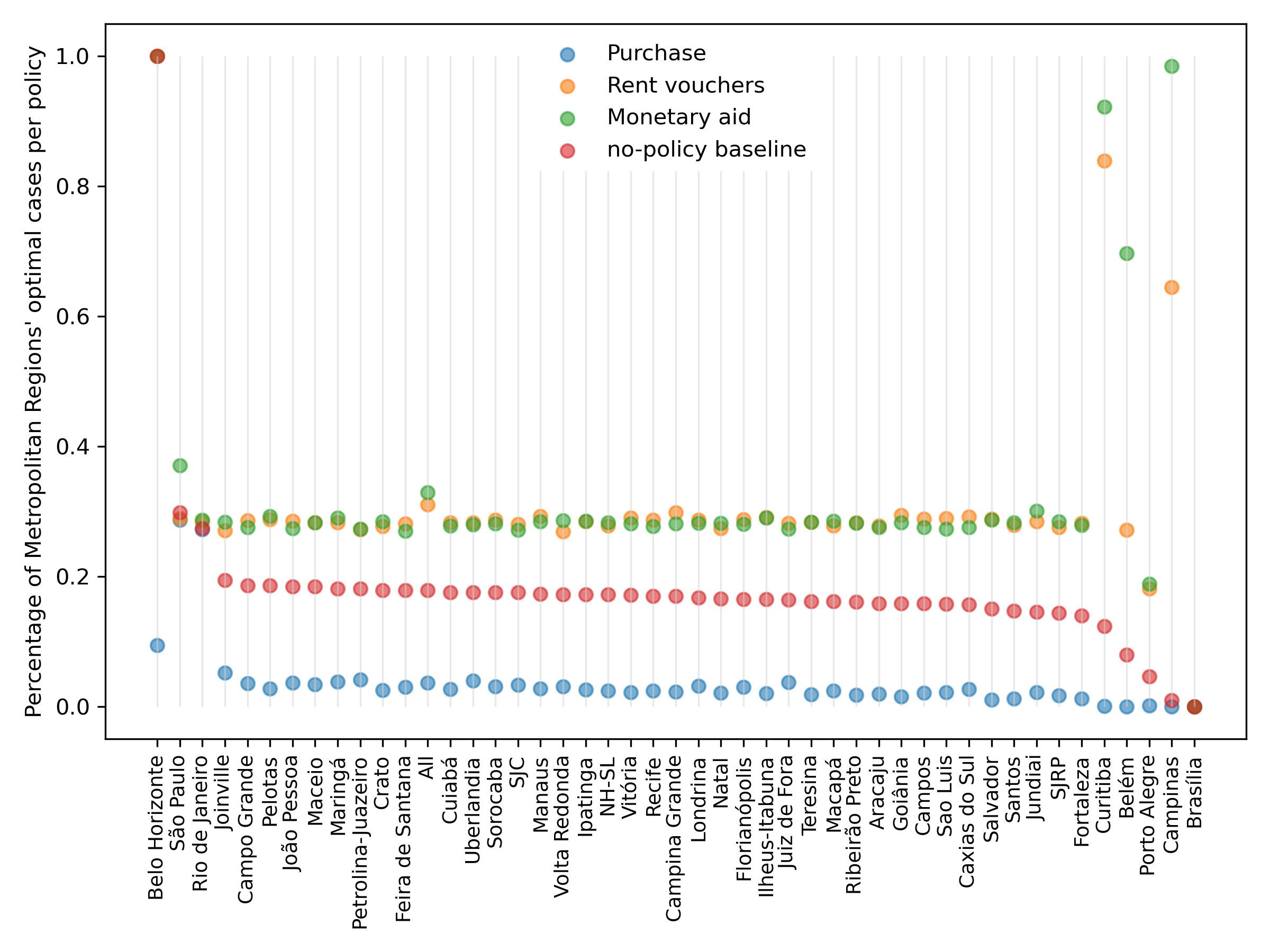
Figure 2: Percentage of optimal cases for the surrogate results, each of the tested policies and the no-policy baseline. The no-policy baseline (in red) clearly separates the mostly negative policy of Property acquisition (blue) and the alternating better policies of Rent vouchers (orange) and Monetary aid (green).

There are some special cases. Given the design and conception of the optimal and their comparative nature across MRs, two cases are extreme. Brasília–the federal capital and host to a number of well-paid civil servants–has the highest structural inequality (Gini coefficient)–of all MRs. Hence, Brasília does not have any classification as optimal in the surrogate, although it accounts for 2.19% of the 1,000,000 runs (see table 6). In the ABM runs, which Brasília accounts for 48.67% of the total, it does reach an optimal case in 1.06% of the time. Our interpretation is not that policymakers should refrain from applying policy in Brasília. Quite on the contrary, applying the policies it would have seem to be not sufficient, given the structural status quo relative to all other MRs.

Conversely, Belo Horizonte seems to benefit from a relatively large GDP, without a largely unequal population (Gini coefficient), thus it reaches the optimal cases in all of the no-policy, Rent vouchers and Monetary aid surrogate runs. Specifically for the case of Belo Horizonte, the Property acquisition policy is especially harmful, reducing the optimal in 90.6 percentage points.

Curitiba, Belém and Campinas are MRs located close to the optimal in such a way that Rent vouchers and Monetary aid would make a huge positive difference within the national comparison. Curitiba would gain nearly 80 percentage points with Monetary aid policy and 71.6 with Rent vouchers. Belém would improve 61.7 with Monetary aid and Campinas would gain more than 95.7 points also with the Monetary aid policy(see table 5).

Table 7 shows the standard-deviation of all MRs, and the average (All). The low level of optimals for the Property acquisition policy is more certain (smaller, more restricted deviation) that for both Rent vouchers and Monetary aid policies. The chance to obtain non-optimal results with the consistently worse policy option (Property acquisition) is higher than the chance to obtain optimal results with the other two options (Monetary aid and Rent vouchers). Hence, it is more certain to fail with Property acquisition than to succeed with either of the other policy instruments.

Property acquisition policy, for most MRs (with the exception of São Paulo and Rio de Janeiro), almost always leads to non-optimal results. Nevertheless, a Property acquisition or Monetary aid policy is not as certain due to the higher standard deviations. This reinforces the understanding that other factors are relevant to determine the outcome of a policy, rather than the policy instrument itself. However, policymakers can be assured that the Property acquisition policy remains as a distant third-best option, unsuited for most MRs and consistently worse than even the no-policy baseline scenario.

4.2 Parameters and rules analysis

The authors of the original ABM model calibrated and validated it towards a reasonable performance along four macroeconomic indicators and the spatial distribution of the real estate market for the city of Brasília in the no-policy baseline scenario alves_furtado2022 . We used the ABM runs’ results to calculate which ones fall into our optimal category, as an ex-post indicator.

The comparative nature of the design differentiates between optimality and non-optimality among the MRs. As such, the results represent the average of the influence of the parameters, rules and policies on the ensemble of all MRs. This helps policymakers comprehend–considering larger and smaller, richer and poorer MRs–direction and intensity of better quality policy.

The optimal of our surrogate ML in turn follows the same (learned) mechanisms of the original ABM, but applies instead a varied parameters’ space. This procedure enables specific parameter values to be associated with optimal/non-optimal results. That is why we consider which parameters and rules (when possible) would need to be modified were policymakers to nudge their MRs towards better results. We used the standardized value for optimal runs to compare the ABM and ML surrogate. There are higher, similar and smaller values of the standard score for the ABM when compared to the ML surrogate optimal (see figure 3).

We could also not reject the null hypothesis that the means were the same for some of the parameters. That indicates that either those parameters were already at an optimal level at the ABM calibration, or that they are not much relevant to generate optimal results.

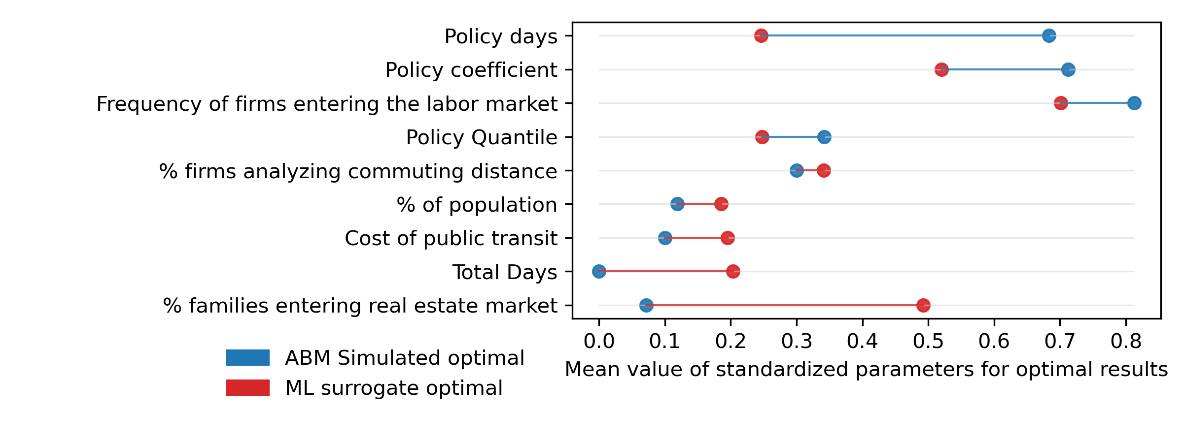
Figure 3: Comparative standard score of parameters for optimal results in relation to the full sample for ABM and ML surrogate runs. We included the parameters for which we could reject the null hypothesis that the means were statistically the same between ABM and ML and also between optimal and non-optimal ML surrogate. The difference from the validated ABM simulation run and the ML surrogate optimal case suggests the counterfactual changes needed in the parameters in order to increase the number of optimal results. The figure is sorted by the difference between ABM Simulated model and ML surrogate optimals.

The three parameters that refer to the design of the size of the households’ set that are to receive policy aid should have smaller values according to the ML surrogate optimal results. Together these parameter optimal values suggest that the choice of families to be included could be more precise and focused. We comment each one in turn.

Policy days refers to the number of days the municipalities look back in time to check the financial conditions of the households and decide whether to include them in the beneficiary pool. The default value is one year (360 days), but the ABM simulation also tested it for 180 days. ML results suggest then that using a smaller number of backward months in order to include households as policy beneficiaries would generate better overall performance.

Policy coefficient specifies the municipalities’ budget share to be invested in the policy. Policy quantile is the income threshold for households to be included in the policy program. Whereas lowering policy coefficient would diminish policy investments, a smaller threshold to include households would probably help focus the policy towards the poorest, most in-need families.

Conversely, note that the Property acquisition policy was by design a policy that helps a comparatively much smaller number of households, given that the amount of financial resources to Property acquisition houses is considerably higher than that of renting, for example. However, in the case of Property acquisition policy, it seems the number of aided households is too small, which is also not the best solution.

The frequency of firms entering the labor market value is slightly lower in the ML surrogate when compared to the ABM model. This suggests that the optimal is reached more frequently when the labor market is less volatile.

The parameter of percentage of firms that analyze commute distance as a criteria in the labor market should be slightly higher to enable more optimal results, according to the ML surrogate model results. This parameter refers to the spatial arrangement of the MRs and varies between hiring exclusively via best candidate qualification or via residence proximity to the hiring firm. As discussed in alves_furtado2022 , it seems that there is a midway arrangement between qualification and commuting distance that best distributes jobs and workers bringing more prosperity for the MR as a whole.

Percentage of population refers to the size of the sample of simulated inhabitants. The higher ML surrogate optimal value depicts the gain that moderately larger MRs have when compared to smaller ones. Total days also indicate that longer simulations may generate more positive feedback effects and help MRs.

The percentage of households that enter the real estate market is much larger in ML surrogate optimal, compared to that of the ABM surrogate optimal. As expected, a more dynamic real estate market indeed brings economic gains to the MRs. It is relevant to highlight, however, that whereas the ABM considers reasonable inflation, along with other macroeconomic indicators, the ML surrogate is concerned with GDP output and Gini coefficient alone. Yet, the parameter value suggests that dynamic real estate markets may bring positive overall results.

Finally, the ML surrogate optimal suggests that cost of public transit should be a bit larger, when compared to the ABM. As the cost of public transit is considered by the candidate as a criteria when deciding the firm to work with, the results may indicate that a better spatial match between workers and firms–mediated via considering more heavily transport costs–might bring more positive results for the full set of the MRs.

Table 2: Comparison of parameters’ absolute values for ABM optimal and ML surrogate optimal results.

Parameters	Standardized values
	ABM optimal	ML surrogate optimal
% firms analyze commute distance	0.300	0.341
% of construction firms	0.200	0.446
% of population	0.118	0.185
% that enters the estate market	0.071	0.492
Cost of private transit	0.500	0.498
Cost of public transit	0.100	0.195
Frequency of firms entering the labor market	0.812	0.701
Hiring sample size	0.655	0.510
Loan/permament income ratio	0.625	0.528
Markup	0.500	0.505
Maximum Loan-to-Value	0.625	0.532
Municipal efficiency management	0.474	0.444
Neighborhood effect	0.571	0.579
Perceived market size	0.474	0.476
Policy Quantile	0.342	0.248
Policy coefficient	0.712	0.520
Policy days	0.683	0.246
Productivity: divisor	0.314	0.566
Productivity: exponent	0.667	0.579
Sticky Prices	0.500	0.489
Supply-demand effect on real estate prices	0.500	0.483
Tax over estate transactions	0.667	0.514
Total Days	0.000	0.204

Table 3: Differences between surrogate and agent-based models in relation to sample size (in % of total simulations), and both optimal and non-optimal cases (% of cases out of the total that fall under each category) for selected dummy parameters of the model.

Rules and Policies’ choices	Size (%)		Optimal (%)		Non-optimal (%)
	Surrogate	ABM	Surrogate	ABM	Surrogate	ABM
Policy: Property acquisition	25.06	12.19	3.62	2.59	96.38	97.41
No-policy baseline	24.93	63.43	17.87	3.91	82.13	96.09
Policy: Rent vouchers	25.01	12.19	31.03	10.37	68.97	89.63
Policy: Monetary aid	25.00	12.19	32.92	13.93	67.08	86.07

4.3 Discussion

In practical terms, the exercise proposed generalizes earlier results and pinpoints which policy is best for which city. Moreover, the robustness of the results confirm that the Property acquisition policy performs worse in terms of GDP and Gini coefficient within a varied input of MRs. Rent vouchers and Monetary aid provide similar results, but may be different for specific MRs.

The federal government (and policymakers) may learn from the analysis performed. The results provide quantitative and empirical data that support alternative emphasis on policy instruments. Typically, Brazilians and OECD members prefer to own their houses causa_housing_2019 . Indeed the Property acquisition program in Brazil was called My House, My Life (PMCMV). However, the program has been criticized by the lack of city integration (distant locations and without infrastructure) santo_amore_minha_2015 , and has virtually stopped due to difficulties in funding. Nationally, no other housing policy has replaced PMCMV. A few studies have recommended rent vouchers as alternatives dias_um_2021 ; rogar_o_2018 . Monetary aid, in turn, has steadily gained support in Brazil fonseca_bolsa_2018 . Our robust results support the novel comparison among housing and social welfare policy instruments making it explicit for policymakers how they compare and what benefits are reached, considering GDP and Gini coefficient as policy goals.

The findings of the surrogate contributes to policy analysis literature by showing that other alternatives (to the Property acquisition policy) not only are available, but also might be more beneficial. PMCMV–the large Property acquisition program in Brazil–was decided upon without observing the planning legislation that was in place, nor the opinion of urban policy experts ferreira_politica_2019 .

The findings of the comparison among the ABM and the ML surrogate optimal results make sense and quantitatively inform policymakers about the direction and intensity of necessary adjustments to replicate optimal MRs performance. All in all, the comparisons suggest: (a) a more focused set of low-income definition of households to assist, (b) with a smaller number of months (of income observation) to include the households, (c) a less volatile (safer) labor market, (d) with a consideration of transport costs to improve the quality of spatial match between firms and employees, (e) and that larger metropolises fair better with increased gains from agglomeration.

5 Concluding remarks

We present a Machine Learning (ML) surrogate model that departs from an ABM model and generalizes its results for a wider number of Metropolitan Regions and policy tests. In the process, we include a much larger, more varied sample of possible input parameters and rules. We also steer the ML surrogate model towards a policy optimum that combines larger GDP output and smaller Gini coefficient within the set of all 46 modeled MRs. Besides the actual findings of best-policy for each MR, the exercise also serves as a test of robustness of the original results.

Considering the research questions, we find that, indeed, different MRs do best in different tested policies. Although on average, the Monetary aid policy performs better, the Rent vouchers is the best policy for a higher number of MRs (24). We further confirm previous results with worst performance for the Property acquisition policy, vis-à-vis those of the no-policy baseline.

Results also showed that some parameters have statistically significant different optimal results in the ML surrogate model and the ABM model. We interpret these values as those the parameters would have to be transformed into, were the MRs to aspire to more socially optimal positions.

The paper presents an exercise to expand the combination of parameters, test the robustness of the results, and evaluate possible pathways for policymakers in terms of which parameters would need changing, were they interested in reaching higher GDP with lower Gini coefficient. However, results are limited by the available data used to produce the surrogate model and the intrinsic validated of the original model itself. Conceptually, we show that a reasonably fast policy evaluation of ABM results–”ex post”–is possible, and one that adds information to policymakers.

In terms of future research, we are interested to learn whether intrinsic Metropolitan Region’ attributes and structural characteristics translates into a higher probability of getting comparatively optimal results. That is, are household attributes and location, number of firms, population qualification and age composition, municipalities boundaries and their geographical interconnections sufficient to determine relative position of one MR in relation to the others? In order to answer such question, we would need to search for the determinants of the optimum, probably via regression techniques.

Moreover, we envision a study that uses dimensionality reduction techniques to summarize a larger number of output indicators to better reflect policymakers preferences. Along with a more comprehensive output indicator, future work should take advantage of the possibilities of mixing simultaneous policy instruments, and those from different domains, such as housing policy and social welfare.

6 Appendices

6.1 Results of other Machine Learning techniques

Besides random forest, we also applied a Multi-layer Perceptron Classifier (MLPC) that optimizes the log-loss function glorot_understanding_2010 , and a C-Support Vector Classification, which relies on a library for Support Vector Machine (libSVM) chang_libsvm_2011 . Finally, we also used a Voting Classifier implementation that uses other model estimators and applies a majority rule voting. See table 4 for confustion matrix results.

Table 4: Confusion matrix for other ML implementation: Multi-layer Perceptron Classifier (MLPC), C-Support Vector Classification (C-SVC), and Voting Classifier.

		Predicted
		Non-optimal	Optimal
Observed MLPC	Non-optimal	2604	0
	Optimal	165	0
Observed C-SVC	Non-optimal	2604	0
	Optimal	165	0
Observed Voting	Non-optimal	2604	0
	Optimal	134	31

6.2 Percentage by policy

See table 5 for the percentage points difference of policies relative to the no-policy baseline.

Table 5: Mean performance of each policy relative to the no-policy baseline for Brazilian MRs. Results for Property acquisition, Rent vouchers and Monetary aid denote performance superior (positive) and inferior (negative) in terms of percentage points, compared to that same MR for the no-policy baseline. All MRs perform worse when policy Property acquisition is applied. Conversely, Monetary aid result in positive performance for all MRs, with varying levels of improvement.

Metropolitan Region \ Policy	%	Difference to the ’no-policy’ scenario (in percentage points)
	No-policy (baseline)	Property acquisition	Rent vouchers	Monetary aid
Belo Horizonte	100.00	-90.58	0.00	0.00
São Paulo	29.84	-1.14	-0.90	7.23
Rio de Janeiro	27.38	-0.12	1.11	1.33
Joinville	19.43	-14.26	7.67	8.91
Campo Grande	18.63	-15.02	10.02	8.91
Pelotas	18.58	-15.81	10.24	10.71
João Pessoa	18.47	-14.78	10.11	8.97
Maceió	18.43	-15.06	9.84	9.83
Maringá	18.14	-14.33	10.16	10.86
Petrolina-Juazeiro	18.11	-13.97	9.16	9.25
Crato	17.92	-15.45	9.81	10.55
Feira de Santana	17.88	-14.90	10.29	9.08
All	17.87	-14.25	13.16	15.05
Cuiabá	17.59	-14.91	10.70	10.21
Uberlandia	17.57	-13.62	10.73	10.39
Sorocaba	17.56	-14.45	11.14	10.60
SJC	17.54	-14.21	10.55	9.59
Manaus	17.30	-14.58	11.94	11.14
Volta Redonda	17.23	-14.12	9.72	11.38
Ipatinga	17.22	-14.61	11.26	11.34
NH-SL	17.21	-14.78	10.61	11.06
Vitória	17.18	-14.97	11.86	10.99
Recife	17.02	-14.62	11.65	10.69
Campina Grande	16.96	-14.73	12.92	11.15
Londrina	16.77	-13.63	11.96	11.48
Natal	16.62	-14.53	10.81	11.59
Florianópolis	16.50	-13.53	12.25	11.57
Ilheus-Itabuna	16.50	-14.49	12.57	12.52
Juiz de Fora	16.40	-12.68	11.81	10.90
Teresina	16.21	-14.34	12.15	12.15
Macapá	16.15	-13.75	11.67	12.36
Ribeirão Preto	16.08	-14.28	12.20	12.16
Aracaju	15.87	-13.97	11.93	11.73
Goiânia	15.86	-14.32	13.58	12.45
Campos	15.83	-13.76	13.06	11.73
Sao Luis	15.73	-13.54	13.22	11.61
Caxias do Sul	15.71	-13.06	13.46	11.89
Salvador	15.04	-14.01	13.83	13.62
Santos	14.67	-13.48	13.20	13.62
Jundiai	14.56	-12.39	13.91	15.50
SJRP	14.36	-12.68	13.23	14.07
Fortaleza	13.99	-12.79	14.26	13.88
Curitiba	12.37	-12.30	71.55	79.85
Belém	8.00	-8.00	19.12	61.69
Porto Alegre	4.62	-4.47	13.50	14.24
Campinas	0.94	-0.94	63.56	97.53
Brasília	0.00	0.00	0.00	0.00
NH-SL: Novo Hamburgo/Sao Leopoldo. SJRP: Sao Jose do Rio Preto.
SJC: Sao Jose dos Campos

6.3 Size, optimal and non-optimal percentages

See table 6 for the sizes of samples, optimal and non-optimal results.

Table 6: Results from surrogate and agent-based models in relation to sample size (in % of total simulations), and both optimal and non-optimal cases (% of cases out of the total that fall under each category) for MRs of the model.

Metropolitan Region	Size (%)		Optimal (%)		Non-optimal (%)
	Surrogate	ABM	Surrogate	ABM	Surrogate	ABM
Aracaju	2.21	1.06	18.16	0.00	81.84	100.00
Belo Horizonte	2.17	2.00	77.06	81.08	22.94	18.92
Belém	2.18	1.06	26.49	21.37	73.51	78.63
Brasília	2.19	48.67	0.00	1.06	100.00	98.94
Campina Grande	2.16	1.06	19.29	0.00	80.71	100.00
Campinas	2.18	2.00	41.01	32.88	58.99	67.12
Campo Grande	2.15	1.06	19.54	0.00	80.46	100.00
Campos	2.17	1.06	18.41	0.00	81.59	100.00
Caxias do Sul	2.18	1.06	18.94	0.00	81.06	100.00
Crato	2.18	1.06	19.07	0.00	80.93	100.00
Cuiabá	2.16	1.06	19.10	0.00	80.90	100.00
Curitiba	2.15	1.06	46.99	47.86	53.01	52.14
Feira de Santana	2.16	1.06	18.89	0.00	81.11	100.00
Florianópolis	2.18	1.06	19.18	0.00	80.82	100.00
Fortaleza	2.17	2.00	17.95	3.15	82.05	96.85
Goiânia	2.16	1.06	18.76	0.00	81.24	100.00
Ilheus-Itabuna	2.18	1.06	19.20	0.00	80.80	100.00
Ipatinga	2.17	1.06	19.25	0.00	80.75	100.00
Joinville	2.16	0.30	19.99	0.00	80.01	100.00
João Pessoa	2.18	1.06	19.52	0.00	80.48	100.00
Juiz de Fora	2.16	1.06	18.78	0.00	81.22	100.00
Jundiai	2.18	1.06	18.80	0.00	81.20	100.00
Londrina	2.18	1.06	19.24	0.00	80.76	100.00
Macapá	2.18	1.06	18.82	0.00	81.18	100.00
Maceio	2.16	1.06	19.66	0.00	80.34	100.00
Manaus	2.17	1.06	19.42	0.00	80.58	100.00
Maringá	2.16	1.06	19.90	0.00	80.10	100.00
NH-SL	2.16	1.06	18.98	0.00	81.02	100.00
Natal	2.19	1.06	18.54	0.00	81.46	100.00
Pelotas	2.16	1.06	19.81	0.00	80.19	100.00
Petrolina-Juazeiro	2.18	1.06	19.21	0.00	80.79	100.00
Porto Alegre	2.20	2.00	10.52	0.00	89.48	100.00
Recife	2.17	1.06	18.92	0.00	81.08	100.00
Ribeirão Preto	2.16	1.06	18.73	0.00	81.27	100.00
Rio de Janeiro	2.19	1.81	27.95	54.73	72.05	45.27
SJC	2.18	1.06	18.95	0.00	81.05	100.00
SJRP	2.17	1.06	17.97	0.00	82.03	100.00
Salvador	2.17	1.06	18.27	11.11	81.73	88.89
Santos	2.17	1.06	18.01	0.00	81.99	100.00
Sao Luis	2.17	1.06	18.53	0.00	81.47	100.00
Sorocaba	2.17	1.06	19.26	0.00	80.74	100.00
São Paulo	2.19	1.06	31.10	100.00	68.90	0.00
Teresina	2.19	1.06	18.81	0.00	81.19	100.00
Uberlandia	2.18	1.06	19.43	0.00	80.57	100.00
Vitória	2.20	1.06	19.20	0.00	80.80	100.00
Volta Redonda	2.16	1.06	19.07	0.00	80.93	100.00
NH-SL: Novo Hamburgo/Sao Leopoldo
SJRP: Sao Jose do Rio Preto
SJC: Sao Jose dos Campos

6.4 Standard-deviation

See table 7 for the standard-deviation of the results for each Metropolitan Region.

6.5 Parameters boundaries configuration

Table 7: Standard deviation of the no-policy baseline compared to policy performance for Brazilian MRs.

Metropolitan Region \ Policy	%	Difference to the ’no-policy’ scenario (in percentage points)
	No-policy (baseline)	Property acquisition	Rent vouchers	Monetary aid
São Paulo	45.75	-0.51	-0.40	2.55
Rio de Janeiro	44.59	-0.06	0.55	0.65
Joinville	39.56	-17.41	4.89	5.51
Campo Grande	38.94	-20.30	6.27	5.73
Pelotas	38.90	-22.48	6.39	6.61
João Pessoa	38.80	-19.95	6.38	5.82
Maceio	38.78	-20.74	6.25	6.25
Maringá	38.54	-19.39	6.51	6.84
Petrolina-Juazeiro	38.51	-18.59	6.02	6.07
Crato	38.35	-22.82	6.42	6.78
Feira de Santana	38.32	-21.31	6.66	6.05
All	38.31	-19.63	7.95	8.68
Cuiabá	38.08	-21.93	6.96	6.72
Uberlandia	38.06	-18.59	6.99	6.82
Sorocaba	38.05	-20.70	7.19	6.93
SJC	38.03	-20.09	6.91	6.43
Manaus	37.82	-21.56	7.67	7.29
Volta Redonda	37.77	-20.41	6.60	7.42
Ipatinga	37.75	-21.81	7.38	7.42
NH-SL	37.75	-22.36	7.06	7.28
Vitória	37.72	-23.02	7.68	7.26
Recife	37.58	-22.28	7.64	7.18
Campina Grande	37.53	-22.75	8.24	7.42
Londrina	37.36	-19.91	7.89	7.66
Natal	37.23	-22.91	7.39	7.77
Florianópolis	37.12	-20.15	8.14	7.81
Ilheus-Itabuna	37.11	-23.08	8.30	8.28
Juiz de Fora	37.03	-18.12	7.97	7.52
Teresina	36.85	-23.30	8.22	8.23
Macapá	36.80	-21.49	8.01	8.35
Ribeirão Preto	36.74	-23.44	8.29	8.28
Aracaju	36.54	-22.87	8.26	8.16
Goiânia	36.53	-24.20	9.05	8.52
Campos	36.50	-22.25	8.82	8.18
Sao Luis	36.41	-21.76	8.94	8.16
Caxias do Sul	36.39	-20.32	9.06	8.31
Salvador	35.75	-25.64	9.57	9.47
Santos	35.38	-24.54	9.45	9.66
Jundiai	35.27	-20.71	9.86	10.58
SJRP	35.07	-22.23	9.63	10.04
Fortaleza	34.69	-23.80	10.33	10.15
Curitiba	32.92	-30.22	3.81	-6.13
Belém	27.12	-27.12	17.34	18.84
Porto Alegre	20.99	-17.11	17.53	18.13
Campinas	9.63	-9.63	38.22	2.64
Brasília	0.00	0.00	0.00	0.00
Belo Horizonte	0.00	29.21	0.00	0.00
NH-SL: Novo Hamburgo/Sao Leopoldo
SJRP: Sao Jose do Rio Preto
SJC: Sao Jose dos Campos

See table 8 for the boundary restrictions for each parameter of the simulation. Each parameter was restricted to possible values, although considering a wider range of variation. For example, markup is bounded between 0 and a 50% increase on prices, considering the default model value of 15%.

We shall briefly explain some parameters, although alves_furtado2022 provides further explanation.

Capped low and top values for the bank refer to the total amount of resources available for the bank.

Policy quantile refers to the size of portion of the poorest families to be included as policy recipients.

Decay factor refers to the loss of property value with time, following equation 1.

$$value=(1-Discount)*e^{Decay*t}+Discount$$ (1)

where, $Discount$ refers to the maximum offer discount, $t$ refers to the time that such property has been on the market, and $Decay$ is the decay factor of property value.

Monthly revenue installments division refers only to construction firms, and it refers to the number of months firms take to incorporate revenue after sales. This is relevant only to determine employees’ wages.

Available lots per Neighbourhood, in the model ”T_LICENSES_PER_REGION” is a monthly designation of licenses for urbanized lots to become available for construction.

Unemployment refers to whether firms observe unemployment or not when setting wages.

Finally, Alternative0 and FPM distribution refer to a previously policy test made by furtado_policyspace:_2018 .

Table 8: Maximum and minimum values or alternatives for simulation parameters.

Parameter	Max	Min
Productivity: exponent	1	0
Productivity: divisor	20	1
Municipal efficiency management	0.001	0.00001
Markup	0.5	0
Sticky Prices	1	0
Perceived market size	100	1
Frequency of firms entering the labor market	1	0
% firms analyzing commuting distance	1	0
Hiring sample size	100	1
Tax: consumption	0.6	0.1
Tax: labor	0.6	0.01
Tax over estate transactions	0.01	0.0001
Tax: firm	0.6	0.01
Tax: property	0.01	0.0001
Policy coefficient	0.4	0
Policy days	3600	0
Policy Quantile	1	0
Age cap for borrower at end of contract	100	50
Loan/permament income ratio	1	0
Maximum Loan-to-Value	1	0
Bank resources: maximum	1	0
Value cap for banks: top	2	1
Value cap for banks: bottom	1	0
Supply-demand effect on real estate prices	5	0
Decay factor for properties	0	-0.1
Maximum offer discount	1	0.4
% families entering real estate market	0.01	0
Neighborhood effect	5	0
Rental Share	1	0
Initial rental price	0.01	0
% of construction firms	0.2	0
Monthly revenue installments division	100	1
Cost of lots (% of construction)	0.7	0
Cost of private transit	0.5	0
Cost of public transit	0.5	0
% of population	1	0
Total Days	14610	1826
Available lots per Neighbourhood	True, False
Starting day	2010-01-01, 2000-01-01
Interest	nominal, real, fixed
Wage is unrelated to unemployment	True, False
Alternative0	True, False
FPM distribution	True, False
Policies	No-policy, Property acquisition, Monetary aid, Rent vouchers

6.6 MRs Data

See table 9 for basic data for each MRs.

Table 9: Basic data from MRs. Total population for MRs from 2010, Municipal Human Development Index (MHDI), and percentage of population with 13 or more years of study. Obs.: Adapted from input data by alves_furtado2022 at github.com/bafurtado/policyspace2/tree/master/input

	Total Population 2010	MHDI	% College $+$
MRs
São Paulo	20,096,809	0.789	0.120
Rio de Janeiro	11,968,973	0.765	0.110
Belo Horizonte	5,039,123	0.769	0.102
Recife	3,706,628	0.732	0.078
Salvador	3,503,340	0.744	0.083
Brasília	3,460,637	0.793	0.110
Fortaleza	3,327,021	0.733	0.073
Curitiba	2,993,678	0.785	0.126
Porto Alegre	2,906,148	0.767	0.120
Campinas	2,603,819	0.792	0.112
Belém	2,125,135	0.730	0.071
Goiânia	2,011,735	0.768	0.106
Manaus	1,802,014	0.737	0.069
Vitória	1,670,679	0.768	0.093
Santos	1,604,363	0.776	0.081
SJC	1,392,552	0.796	0.108
São Luis	1,309,330	0.754	0.072
Natal	1,251,459	0.740	0.083
Sorocaba	1,148,035	0.783	0.096
Maceió	1,028,249	0.713	0.094
João Pessoa	1,017,742	0.732	0.100
Teresina	982,968	0.733	0.085
Aracaju	879,061	0.731	0.087
Florianópolis	866,098	0.812	0.148
Cuiabá	803,694	0.769	0.105
Ribeirão Preto	791,295	0.788	0.137
Campo Grande	786,797	0.784	0.117
Joinville	748,470	0.799	0.107
NH-SL	736,405	0.739	0.057
Londrina	709,494	0.765	0.109
Jundiaí	674,877	0.795	0.106
Uberlândia	604,013	0.789	0.109
Volta Redonda	579,427	0.747	0.086
Feira de Santana	556,642	0.712	0.042
Maringá	546,408	0.776	0.109
Juiz de Fora	532,474	0.776	0.127
Pelotas	525,503	0.741	0.091
SJRP	502,494	0.789	0.128
Macapá	499,466	0.725	0.068
Caxias do Sul	499,199	0.781	0.096
Petrolina-Juazeiro	491,927	0.689	0.049
Ipatinga	468,378	0.758	0.067
Campos	463,731	0.716	0.046
Campina Grande	452,162	0.705	0.071
Crato	426,690	0.698	0.048
Ilhéus-Itabuna	388,903	0.702	0.054
NH-SL: Novo Hamburgo/Sao Leopoldo
SJRP: Sao Jose do Rio Preto
SJC: Sao Jose dos Campos

References

- \bibcommenthead
- (1) Stone, D.: Understanding the transfer of policy failure: bricolage, experimentalism and translation. Policy & Politics 45(1), 55–70 (2017). https://doi.org/10.1332/030557316X14748914098041
- (2) Mitchell, C., Woodman, B.: Regulation and sustainable energy systems. In: Baldwin, R., Cave, M., Lodge, M. (eds.) The Oxford Handbook of Regulation, pp. 573–590. Oxford University press, Oxford (2010)
- (3) Gawel, E., Strunz, S., Lehmann, P.: Support Policies for Renewables Instrument Choice and Instrument Change from a Public Choice Perspective. United Nations University World Institute for Development Economics Research, Helsinki, Finland (2016)
- (4) Cravo, T.A., Resende, G.M.: Economic growth in Brazil: a spatial filtering approach. The Annals of Regional Science 50(2), 555–575 (2013). https://doi.org/10.1007/s00168-012-0504-6. Accessed 2022-01-28
- (5) Boschma, R.: Constructing Regional Advantage and Smart Specialization: Comparison of Two European Policy Concepts. Papers in Evolutionary economic geography 13(22) (2013)
- (6) Lundvall, B.: National Innovation Systems—Analytical Concept and Development Tool. Industry & Innovation 14(1), 95–119 (2007). https://doi.org/10.1080/13662710601130863
- (7) Mueller, B.: Why public policies fail: Policymaking under complexity. EconomiA 21(2), 311–323 (2020). https://doi.org/10.1016/j.econ.2019.11.002. Accessed 2022-01-28
- (8) Nelson, R.R.: The co-evolution of technology, industrial structure, and supporting institutions. Industrial and Corporate Change 3(1) (1994)
- (9) Hochstetler, K., Kostka, G.: Wind and Solar Power in Brazil and China: Interests, State–Business Relations, and Policy Outcomes. Global Environmental Politics 15(3), 74–94 (2015). https://doi.org/10.1162/GLEP_a_00312
- (10) Faber, A., Valente, M., Janssen, P.: Exploring domestic micro-cogeneration in the Netherlands: An agent-based demand model for technology diffusion. Energy Policy 38(6), 2763–2775 (2010). https://doi.org/10.1016/j.enpol.2010.01.008
- (11) Tesfatsion, L.: Agent-based Modeling and Institutional Design. Eastern Economic Journal 37(1), 13–19 (2011). https://doi.org/10.1057/eej.2010.34
- (12) Calder, M., Craig, C., Culley, D., de Cani, R., Donnelly, C.A., Douglas, R., Edmonds, B., Gascoigne, J., Gilbert, N., Hargrove, C., Hinds, D., Lane, D.C., Mitchell, D., Pavey, G., Robertson, D., Rosewell, B., Sherwin, S., Walport, M., Wilson, A.: Computational modelling for decision-making: where, why, what, who and how. Royal Society Open Science 5(6), 172096 (2018) https://royalsocietypublishing.org/doi/pdf/10.1098/rsos.172096. https://doi.org/10.1098/rsos.172096
- (13) de Marchi, S., Page, S.E.: Agent-Based Models. Annual Review of Political Science 17(1), 1–20 (2014). https://doi.org/10.1146/annurev-polisci-080812-191558
- (14) Lamperti, F., Dosi, G., Napoletano, M., Roventini, A., Sapio, A.: Faraway, So Close: Coupled Climate and Economic Dynamics in an Agent-based Integrated Assessment Model. Ecological Economics 150, 315–339 (2018). https://doi.org/10.1016/j.ecolecon.2018.03.023
- (15) Lespagnol, V., Rouchier, J.: Trading Volume and Price Distortion: An Agent-Based Model with Heterogenous Knowledge of Fundamentals. Computational Economics 51(4), 991–1020 (2018). https://doi.org/10.1007/s10614-017-9655-y
- (16) Huang, W., Zheng, H., Chia, W.-M.: Financial crises and interacting heterogeneous agents. Journal of Economic Dynamics and Control 34(6), 1105–1122 (2010). https://doi.org/10.1016/j.jedc.2010.01.013
- (17) Arthur, W.B.: Inductive reasoning and bounded rationality. The American Economic Review 84(2), 406–411 (1994)
- (18) Brenner, T., Werker, C.: Policy advice derived from simulation models. Journal of Artificial Societies and Social Simulation 12(4), 2 (2009)
- (19) Schmidt, T.S., Battke, B., Grosspietsch, D., Hoffmann, V.H.: Do deployment policies pick technologies by (not) picking applications?—A simulation of investment decisions in technologies with multiple applications. Research Policy 45(10), 1965–1983 (2016). https://doi.org/10.1016/j.respol.2016.07.001
- (20) Tesfatsion, L.: Agent-based computational economics: Modeling economies as complex adaptive systems. Information Sciences 149(4), 262–268 (2003). https://doi.org/10.1016/S0020-0255(02)00280-3
- (21) Arthur, W.B.: Out-of-equilibrium economics and agent-based modeling. In: Tesfatsion, L., Judd, K.L. (eds.) Handbook of Computational Economics vol. 2, pp. 1551–1564. Elsevier, Berlin (2006). https://doi.org/10.1016/S1574-0021(05)02032-0. https://linkinghub.elsevier.com/retrieve/pii/S1574002105020320 Accessed 2019-07-02
- (22) Axelrod, R.M.: The Complexity of Cooperation: Agent-Based Models of Competition and Collaboration. Princeton Studies in Complexity. Princeton University Press, Princeton, N.J (1997)
- (23) Janssen, M., Ostrom, E.: Empirically based, agent-based models. Ecology and Society 11(2), 1–13 (2006)
- (24) Epstein, J.M., Axtell, R.: Growing Artificial Societies: Social Science from the Bottom Up. Brookings/MIT Press, Cambridge, MA (1996)
- (25) Vazquez, M., Hallack, M.: The role of regulatory learning in energy transition: The case of solar PV in Brazil. Energy Policy 114, 465–481 (2018). https://doi.org/10.1016/j.enpol.2017.11.066
- (26) Galán, J.M., Izquierdo, L.R., Izquierdo, S.S., Santos, J.I., Olmo, R.d., López-Paredes, A., Edmonds, B.: Errors and Artefacts in Agent-Based Modelling. Journal of Artificial Societies and Social Simulation 12(1) (2009)
- (27) Chen, S.-H., Lux, T., Marchesi, M.: Testing for non-linear structure in an artificial financial market. Journal of Economic Behavior & Organization 46, 327–342 (2001)
- (28) Ehrentreich, N.: The Original Santa Fe Institute Artificial Stock Market. Lecture Notes in Economics and Mathematical Systems, pp. 91–112. Springer, Berlin (2008)
- (29) Alves Furtado, B.: Policyspace2: Modeling markets and endogenous public policies. Journal of Artificial Societies and Social Simulation 25(1), 8 (2022). https://doi.org/10.18564/jasss.4742
- (30) Paleyes, A., Pullin, M., Mahsereci, M., McCollum, C., Lawrence, N.D., Gonzalez, J.: Emulation of physical processes with Emukit. In: Second Workshop on Machine Learning and the Physical Sciences (2019). arXiv: 2110.13293. http://arxiv.org/abs/2110.13293 Accessed 2022-01-28
- (31) van der Hoog, S.: Surrogate Modelling in (and of) Agent-Based Models: A Prospectus. Computational Economics 53(3), 1245–1263 (2019-03). https://doi.org/10.1007/s10614-018-9802-0. Accessed 2021-10-25
- (32) ten Broeke, G., van Voorn, G., Ligtenberg, A., Molenaar, J.: The Use of Surrogate Models to Analyse Agent-Based Models. Journal of Artificial Societies and Social Simulation 24(2), 3 (2021). https://doi.org/10.18564/jasss.4530. Accessed 2021-10-12
- (33) Furtado, B.A., Sakowski, P.A.M., Tóvolli, M.H.: Modeling Complex Systems for Public Policies. IPEA, Brasília (2015)
- (34) Geyer, R., Cairney, P.: Handbook on Complexity and Public Policy. Handbooks of Research on Public Policy series. Edward Elgar Publishing, Northampton, Massachusetts (2015)
- (35) Gilbert, N., Ahrweiler, P., Barbrook-Johnson, P., Narasimhan, K.P., Wilkinson, H.: Computational Modelling of Public Policy: Reflections on Practice. Journal of Artificial Societies and Social Simulation 21(1), 14 (2018)
- (36) Edmonds, B., Meyer, R. (eds.): Simulating Social Complexity: A Handbook, 2nd edn. Understanding Complex Systems. Springer, New York City (2017). https://doi.org/10.1007/978-3-319-66948-9. https://www.springer.com/gp/book/9783319669472 Accessed 2021-01-05
- (37) Lee, J.-S., Filatova, T., Ligmann-Zielinska, A., Hassani-Mahmooei, B., Stonedahl, F., Lorscheid, I., Voinov, A., Polhill, J.G., Sun, Z., Parker, D.C.: The Complexities of Agent-Based Modeling Output Analysis. Journal of Artificial Societies and Social Simulation 18(4), 4 (2015)
- (38) Heppenstall, A.J., Crooks, A.T., See, L.M., Batty, M.: Agent-Based Models of Geographical Systems. Springer, New York City (2012)
- (39) Dawid, H., Gatti, D.D.: Agent-Based Macroeconomics. In: Handbook on Computational Economics vol. IV. Elsevier, Amsterdam (2018)
- (40) Adepetu, A., Keshav, S., Arya, V.: An agent-based electric vehicle ecosystem model: San Francisco case study. Transport Policy 46, 109–122 (2016). https://doi.org/10.1016/j.tranpol.2015.11.012. Accessed 2019-05-02
- (41) Scott, N., Livingston, M., Hart, A., Wilson, J., Moore, D., Dietze, P.: SimDrink: An Agent-Based NetLogo Model of Young, Heavy Drinkers for Conducting Alcohol Policy Experiments. Journal of Artificial Societies and Social Simulation 19(1), 10 (2016)
- (42) Ingham-Dempster Tim, Walker Dawn C., Corfe Bernard M.: An agent-based model of anoikis in the colon crypt displays novel emergent behaviour consistent with biological observations. Royal Society Open Science 4(4), 160858 (2017). https://doi.org/10.1098/rsos.160858. Accessed 2019-05-02
- (43) van der Veen, R.A.C., Kisjes, K.H., Nikolic, I.: Exploring policy impacts for servicising in product-based markets: A generic agent-based model. Journal of Cleaner Production 145, 1–13 (2017). https://doi.org/10.1016/j.jclepro.2017.01.016. Accessed 2019-05-02
- (44) Carley, K.M., Fridsma, D.B., Casman, E., Yahja, A., Altman, N., Chen, L.-C., Kaminsky, B., Nave, D.: BioWar: scalable agent-based model of bioattacks. IEEE Transactions on Systems, Man, and Cybernetics - Part A: Systems and Humans 36(2), 252–265 (2006). https://doi.org/10.1109/TSMCA.2005.851291. Conference Name: IEEE Transactions on Systems, Man, and Cybernetics - Part A: Systems and Humans
- (45) Kerr, C.C., Stuart, R.M., Mistry, D., Abeysuriya, R.G., Rosenfeld, K., Hart, G.R., Núñez, R.C., Cohen, J.A., Selvaraj, P., Hagedorn, B., George, L., Jastrzebski, M., Izzo, A.S., Fowler, G., Palmer, A., Delport, D., Scott, N., Kelly, S.L., Bennette, C.S., Wagner, B.G., Chang, S.T., Oron, A.P., Wenger, E.A., Panovska-Griffiths, J., Famulare, M., Klein, D.J.: Covasim: An agent-based model of COVID-19 dynamics and interventions. PLOS Computational Biology 17(7), 1009149 (2021). https://doi.org/10.1371/journal.pcbi.1009149. Publisher: Public Library of Science. Accessed 2021-08-26
- (46) Ahrweiler, P., Schilperoord, M., Pyka, A., Gilbert, N.: Modelling Research Policy: Ex-Ante Evaluation of Complex Policy Instruments. Journal of Artificial Societies and Social Simulation 18(4), 5 (2015)
- (47) Aodha, L.n., Edmonds, B.: Some pitfalls to beware when applying models to issues of policy relevance. In: Simulating Social Complexity, a Handbook, 2nd edn. Understanding Complex Systems, pp. 801–822. Springer, Berlin (2017)
- (48) Breiman, L.: Random forests. Machine learning 45, 5–32 (2001)
- (49) van Engelen, J.E., Hoos, H.H.: A survey on semi-supervised learning. Machine Learning 109(2), 373–440 (2020). https://doi.org/10.1007/s10994-019-05855-6. Accessed 2022-08-29
- (50) Wiering, M.A., Van Otterlo, M.: Reinforcement Learning. Adaptation, Learning, and Optimization, vol. 12. Springer, ??? (2012). Publisher: Springer
- (51) Ren, Q., Cheng, H., Han, H.: Research on machine learning framework based on random forest algorithm. AIP Conference Proceedings 1820(1), 080020 (2017). https://doi.org/10.1063/1.4977376. Publisher: American Institute of Physics. Accessed 2022-04-14
- (52) Mishina, Y., Murata, R., Yamauchi, Y., Yamashita, T., Fujiyoshi, H.: Boosted Random Forest. IEICE Transactions on Information and Systems E98.D(9), 1630–1636 (2015). https://doi.org/10.1587/transinf.2014OPP0004. Accessed 2021-10-25
- (53) Lavin, A., Zenil, H., Paige, B., Krakauer, D., Gottschlich, J., Mattson, T., Anandkumar, A., Choudry, S., Rocki, K., Baydin, A.G., Prunkl, C., Paige, B., Isayev, O., Peterson, E., McMahon, P.L., Macke, J., Cranmer, K., Zhang, J., Wainwright, H., Hanuka, A., Veloso, M., Assefa, S., Zheng, S., Pfeffer, A.: Simulation Intelligence: Towards a New Generation of Scientific Methods. arXiv:2112.03235 [cs] (2021). arXiv: 2112.03235. Accessed 2022-01-12
- (54) Lamperti, F., Roventini, A., Sani, A.: Agent-based model calibration using machine learning surrogates. Journal of Economic Dynamics and Control 90, 366–389 (2018-05). https://doi.org/10.1016/j.jedc.2018.03.011. Accessed 2021-10-12
- (55) Conti, S., O’Hagan, A.: Bayesian emulation of complex multi-output and dynamic computer models. Journal of Statistical Planning and Inference 140(3), 640–651 (2010-03). https://doi.org/10.1016/j.jspi.2009.08.006. Accessed 2021-10-25
- (56) Hayashi, S., Prasasti, N., Kanamori, K., Ohwada, H.: Improving behavior prediction accuracy by using machine learning for agent-based simulation. In: Nguyen, N.T., Trawiński, B., Fujita, H., Hong, T.-P. (eds.) Intelligent Information and Database Systems. Lecture Notes in Computer Science, vol. 9621, pp. 280–289. Springer, Berlin, Heidelberg (2016). https://doi.org/10.1007/978-3-662-49381-6_27. http://link.springer.com/10.1007/978-3-662-49381-6_27 Accessed 2021-10-12
- (57) Edali, M., Yücel, G.: Exploring the behavior space of agent-based simulation models using random forest metamodels and sequential sampling. Simulation Modelling Practice and Theory 92, 62–81 (2019-04). https://doi.org/10.1016/j.simpat.2018.12.006. Accessed 2021-10-11
- (58) Guerrero, O.A., Castañeda, G.: Policy priority inference: A computational framework to analyze the allocation of resources for the sustainable development goals. Data & Policy 2 (2020). https://doi.org/10.1017/dap.2020.18. Publisher: Cambridge University Press. Accessed 2022-03-03
- (59) Guerrero, O.A., Castañeda, G.: How does government expenditure impact sustainable development? Studying the multidimensional link between budgets and development gaps. Sustainability Science (2022). https://doi.org/10.1007/s11625-022-01095-1. Accessed 2022-03-03
- (60) Austin, A.: On Well-Being and Public Policy: Are We Capable of Questioning the Hegemony of Happiness? Social Indicators Research 127(1), 123–138 (2016). https://doi.org/10.1007/s11205-015-0955-0. Accessed 2022-03-03
- (61) Causa, O., Woloszko, N., Leite, D.: Housing, wealth accumulation and wealth distribution: Evidence and stylized facts. Technical Report 1588, Organisation for Economic Co-operation and Development, Paris, France (December 2019). Publisher: OECD
- (62) Santo Amore, C., Shimbo, L.Z., Rufino, M.B.C.: Minha Casa… E a Cidade? Avaliação do Programa Minha Casa Minha Vida em seis estados brasileiros. Rio de Janeiro: Letra Capital (2015)
- (63) Dias, D.M.d.S., Santos, J.C.d.: Um estudo acerca do aluguel social como instrumento de acesso ao direito à moradia digna diante do déficit de habitação no Brasil / A study about social rent as an instrument for access to the right to decent housing in light of the housing deficit in Brazil. Revista de Direito da Cidade 13(3), 1631–1659 (2021). https://doi.org/10.12957/rdc.2021.45239. Number: 3. Accessed 2022-09-05
- (64) Rogar, R., Vieira, P.R.S.: O aluguel social como instrumento perene de dignificação da pessoa humana. Revista de Direito da Cidade 10(4), 2259–2288 (2018)
- (65) Fonseca, A., Jaccoud, L., Karam, R.: Do Bolsa Família ao Brasil sem Miséria: o desafio de universalizar a cidadania. Protecao social e transferencia de renda. Caderno de Pesquisa NEPP (86), 52–79 (2018)
- (66) Ferreira, G.G., Calmon, P., Fernandes, A.S.A., Araújo, S.M.V.G.d.: Política habitacional no Brasil: uma análise das coalizões de defesa do Sistema Nacional de Habitação de Interesse Social versus o Programa Minha Casa, Minha Vida. urbe. Revista Brasileira de Gestão Urbana 11 (2019). https://doi.org/10.1590/2175-3369.011.001.AO04. Publisher: Pontifícia Universidade Católica do Paraná. Accessed 2022-09-05
- (67) Glorot, X., Bengio, Y.: Understanding the difficulty of training deep feedforward neural networks. In: Proceedings of the Thirteenth International Conference on Artificial Intelligence And Statistics, pp. 249–256. JMLR Workshop and Conference Proceedings, ??? (2010). ISSN: 1938-7228. https://proceedings.mlr.press/v9/glorot10a.html Accessed 2022-09-02
- (68) Chang, C.-C., Lin, C.-J.: LIBSVM: a library for support vector machines. ACM transactions on intelligent systems and technology (TIST) 2(3), 1–27 (2011). Publisher: Acm New York, NY, USA
- (69) Furtado, B.A.: PolicySpace: a modeling platform. Journal on Policy and Complex Systems 4(2), 17–30 (2018). https://doi.org/10.18278/jpcs.4.2.3