Thermal drag effect in quantum Hall circuits

Abstract

We study the thermal drag between two mesoscopic quantum Hall (QH) circuits. Each circuit consists of Ohmic contact perfectly coupled to quantum Hall edge states. The drag is caused by strong capacitive coupling between Ohmic contacts. The non-equilibirum conditions and the electron-electron interaction are taken into account by using the non-equilibrium bosonization technique. The thermal drag current in the passive circuit, the noise power of the corresponding heat current, and the Fano factor are calculated and analyzed.

The mutual electron drag effect is the phenomenon that arises in a system of two isolated (in the absence of the transfer of charge) quantum circuits coupled via the long-range Coulomb interaction [1]. Typically, one is interested in the so-called Coulomb drag effect, where the charge current in the “active” part of the circuit causes the charge drag current in the “passive” part of the circuit [2], and normally, this effect is perturbative and weak. The Coulomb drag effect in various systems was thoroughly studied both experimentally and theoretically [1]. It was further shown that the charge drag current can also be mediated by the combined electron-phonon, electron-photon, and electron-ion interactions [3, 4, 5]. All these effect have to be differentiated with the thermal drag effect, which can also be cause by the long-range Coulomb interaction [6, 7, 8, 9]. In this case the flow of heat current in the active circuit results in the heat current in the passive circuit. Of particular interest is the thermal drag effect due to the temperature difference between active and passive circuits. The effect of thermal drag was studied in the context of quantum refrigerators and engines, heat diodes and heat pumps [10, 11, 12, 13, 14, 15].

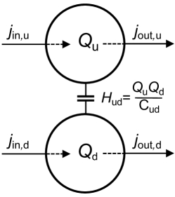
Figure 1: Schematic of the possible experimental setup. The systems consists of two identical quantum circuits: upper (active) and lower (passive) parts. Each part includes an Ohmic contact (metallic granula with capacitance $C$ and negligible level spacing) which is perfectly coupled to chiral integer QH channel (the channel enters an Ohmic contact and leaves it without electron backscattering). The incoming channels are kept at different temperatures $T_{\rm in,u}-T_{\rm in,d}>0$. The capacitive coupling between Ohmic contacts, $Q_{\rm u}Q_{\rm d}/C_{\rm ud}$, results in thermal drag effect: The upper mesoscopic circuit induces extra heat current in the lower circuit in the outgoing channel.

The recent progress in the fabrication of hybrid systems that are based on chiral QH edge states made it possible to do accurate mesoscopic experiments with strongly interacting electron systems [16]. A particular interesting example of such system is a QH edge state perfectly coupled to an Ohmic contact, a mesoscale metallic granula with negligible level spacing and finite charging energy comparable to the temperature [17]. It is worth mentioning that such an Ohmic contact immediately became a key element of new experimental and theoretical studies [16], the remarkable examples being the suppression of charge quantization caused by quantum and thermal fluctuations [18, 19], the heat Coulomb blockade effect [20, 21, 22, 23], the interaction induced recovery of the phase coherence [24, 25, 26], the charge Kondo effect [27, 28], the quantization of the anyonic heat flow [29], and the observation of the half-integer thermal Hall conductance [30, 31].

In this Letter, we propose a mesoscopic QH system with embedded Ohmic contacts, building up strong Coulomb interactions, for studying thermal drag effect (see Fig. 1). The system consists of the active (upper) and passive (lower) quantum circuits. Each circuit includes an Ohmic contact perfectly coupled to a chiral QH edge state: The edge state enters an Ohmic contact and leaves it without electron backscattering. The thermal drag effect is caused by the capacitive coupling between Ohmic contacts of the active and passive circuits. The temperature difference $T_{\rm in,u}-T_{\rm in,d}>0$ is applied between circuits which causes the temperature imbalance between contacts and results in the thermal heat flow from the upper to the lower part. We assume the full thermalization of the electron systems inside Ohmic contacts. In our study we focus on the thermal drag current, its zero-frequency noise power, and the associated Fano factor.

Model and theoretical approach. We use the low-energy effective field theory [32, 33] to describe QH edge states strongly coupled to the Ohmic contacts. The Ohmic contact is modeled by extending an edge state inside the metallic granula and splitting it in two uncorrelated channels [20, 21]. The Hamiltonian of each quantum circuit ($\alpha=\rm u,d$) contains two terms (see Fig. 2)

$$\begin{split}&H_{\alpha}=\frac{v_{F}}{4\pi}\sum_{\sigma=\pm}\int dx(\partial_{x}\phi_{\alpha\sigma})^{2}+Q^{2}_{\alpha}/2C,\\ &Q_{\alpha}=\int_{-\infty}^{0}dxe^{\epsilon x/v_{F}}\left[\rho_{\alpha+}(x)+\rho_{\alpha-}(x)\right],\end{split}$$ (1)

where $v_{F}$ is Fermi velocity, $C$ is capacitance of each Ohmic contact, $Q_{\alpha}$ is an operator of the total charge accumulated at each Ohmic contact, and $\epsilon$ is a small regularization parameter. Here the first term accounts for the dynamics of incoming and outgoing edge channels, and the second term describes the charging energy of an Ohmic contact of a finite size. The set of scalar fields $\phi_{\alpha\sigma}(x,t)$, where $\alpha=\rm u,d$ and $\sigma=\pm$, are introduced in Eq. (1) to describe the low energy physics. The operators of edge charge densities and currents for incoming, $\sigma=-$, and outgoing, $\sigma=+$, states are given by $\rho_{\alpha\sigma}=(1/2\pi)\partial_{x}\phi_{\alpha\sigma}$ and $j_{\alpha\sigma}=-(1/2\pi)\partial_{t}\phi_{\alpha\sigma}$. The bosonic fields satisfy the standard canonical commutation relations

$$[\partial_{x}\phi_{\alpha\sigma}(x,t),\phi_{\alpha^{\prime}\sigma^{\prime}}(x^{\prime},t)]=2\pi i\sigma\delta_{\alpha\alpha^{\prime}}\delta_{\sigma\sigma^{\prime}}\delta(x-x^{\prime}),$$ (2)

where $\delta_{\alpha\alpha^{\prime}}$ is the Kronecker delta and $\delta(x)$ is the Dirac delta function. It is worth mentioning that the presented above model of an Ohmic contact was successfully used to explained the experiments on the charge quantization, heat Coulomb blockade and heat quantization of anyonic flow [18, 22, 23, 29, 30, 31].

The total Hamiltonian of the system includes three terms (see Fig. 1)

$$H=H_{\rm u}+H_{\rm d}+H_{\rm ud},$$ (3)

where the Hamiltonians of the active and passive circuit, $H_{\alpha}$, are given in Eq. (1), while capacitive coupling between Ohmic contacts has the form

$$H_{\rm ud}=Q_{\rm u}Q_{\rm d}/C_{\rm ud},$$ (4)

where $1/C_{\rm ud}$ is mutual capacitive coupling constant.

Using commutation relations from Eq. (2), the Hamiltonian (1) and (3), and the definition of the current operators

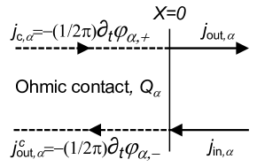
Figure 2: The model of an Ohmic contact with the capacitive interaction is illustrated, see Eq. (1). The charge current $j_{\rm in,\alpha}(t)$ arriving at the Ohmic contact enters it at the interface at $x=0$ and continues as a neutral current $j^{\rm c}_{\rm out,\alpha}(t)$. The neutral current $j^{\rm c}_{\alpha}(t)$ arriving at the interface from inside the Ohmic contact continues as a charge current $j_{\rm out,\alpha}(t)$. In order to account for the negligible level spacing in the Ohmic contact, we extend edge states inside it to minus infinity and introduce the small regularization parameter $\epsilon$ in Eq. (1).

one can present the equations of motion for the currents and the charges in a form of Langevin equations [21, 19], namely

$$\begin{split}&\partial_{t}Q_{\alpha}(t)=j_{\rm in,\alpha}(t)-j_{\rm out,\alpha}(t),\\ &j_{\rm out,\alpha}(t)=[Q_{\alpha}(t)+\lambda Q_{-\alpha}(t)]/\tau_{\rm c}+j_{\rm c,\alpha}(t),\\ &j_{\rm out,\alpha}(t)+j^{\rm c}_{\rm out,\alpha}(t)=j_{\rm in,\alpha}(t)+j_{\rm c,\alpha}(t),\end{split}$$ (5)

where $\lambda=C/C_{\rm ud}\leq 1$ is the dimensionless coupling constant, $\tau_{\rm c}=R_{\rm q}C$ is the charge relaxation time, $R_{\rm q}=2\pi\hbar/e^{2}$ is the resistance quantum, and $-\alpha=\rm d,u$ simply denotes swapping the indexes $\alpha=\rm u,d$. Here, the first equation expresses the conservation of charge in the circuit $\alpha$. The second line is the Langevin equation, which has the simple meaning: The outgoing current acquires one contributions $[Q_{\alpha}(t)+\lambda Q_{-\alpha}(t)]/\tau_{\rm c}$ from the time dependent potential of an Ohmic contact $\alpha$, and the second contribution $j_{\rm c,\alpha}$ that can be viewed as a Langevin source. The third equation expresses the conservation of incoming and outgoing currents at each Ohmic contact.

The Eqs. (5) can be easily solved, and the results may be presented as

$$\mathbf{J}_{\rm out}(\omega)=\mathcal{\hat{U}}(\omega)\mathbf{J}_{\rm in}(\omega),$$ (6)

where the four component vectors of outgoing and incoming currents are given by $\mathbf{J}_{\rm out}=(j_{\rm out,u},j_{\rm out,d},j^{\rm c}_{\rm out,u},j^{\rm c}_{\rm out,d})$, and $\mathbf{J}_{\rm in}=(j_{\rm in,u},j_{\rm in,d},j_{\rm c,u},j_{\rm c,d})$ The scattering matrix in Eq. (6) has the form

$$\mathcal{\hat{U}}(\omega)=\begin{bmatrix}\mathcal{A}&\mathcal{B}&\mathcal{C}&-\mathcal{B}\\ \mathcal{B}&\mathcal{A}&-\mathcal{B}&\mathcal{C}\\ \mathcal{C}&-\mathcal{B}&\mathcal{A}&\mathcal{B}\\ -\mathcal{B}&\mathcal{C}&\mathcal{B}&\mathcal{A}\end{bmatrix},$$ (7)

where $\mathcal{A}(\omega)=[i\omega\tau_{\rm c}+\lambda^{2}-1]/[(\omega\tau_{\rm c}+i)^{2}+\lambda^{2}]$, $\mathcal{B}(\omega)=i\lambda\omega\tau_{\rm c}/[(\omega\tau_{\rm c}+i)^{2}+\lambda^{2}]$, and $\mathcal{C}(\omega)=\omega\tau_{\rm c}[\omega\tau_{\rm c}+i]/[(\omega\tau_{\rm c}+i)^{2}+\lambda^{2}]$. One can easily check the unitary of the scattering matrix: $\mathcal{\hat{U}}^{\dagger}(\omega)=\mathcal{\hat{U}}(\omega)^{-1}$, which reflects the conservative character of the equations of motion, before Langevin sources are traced out. It is also worth mentioning that at $\lambda=0$ or $1$ one recovers the results for scattering matrix obtained in Refs. [21, 19, 25].

Next, we assume that currents originating from Ohmic contacts are equilibrium. Thus, the two-point correlation functions of the incoming currents as well as the Langevin sources are given by the equilibrium spectral function [34]

$$\langle\delta j_{l,\alpha}(\omega)\delta j_{k,\beta}(\omega^{\prime})\rangle=2\pi\delta_{lk}\delta_{\alpha\beta}\delta(\omega+\omega^{\prime})S_{l,\alpha}(\omega),$$ (8)

where $S_{l,\alpha}(\omega)=R^{-1}_{\rm q}\omega/(1-e^{-\omega/T_{l,\alpha}})$ and $l,k={\rm in,c}$, and $\alpha,\beta=\rm u,d$. These correlation functions are used for further calculations. Note, however, the temperatures of Ohmic contacts $T_{\rm c,u/d}$ are yet unknown. They will be found below.

Heating effect and thermal drag current. In a chiral QH channel, the energy current operator is equal to the energy density operator multiplied by group velocity ${\cal J}_{l,\alpha}(t)=(v^{2}/4\pi)[\partial_{x}\phi_{l,\alpha}(x,t)]^{2}$. Using the equation of motion for the bosonic field, $\phi_{l,\alpha}(x,t)$, one can rewrite the energy current as ${\cal J}_{l,\alpha}(t)=(R_{\rm q}/2)j^{2}_{l,\alpha}(t),$ where $j_{l,\alpha}(t)$ are given in Eqs. (5) and (6). The heat current can be obtained by subtracting the vacuum (zero temperature) contribution:

$$J_{l,\alpha}=(R_{\rm q}/2)[\langle j^{2}_{l,\alpha}\rangle-\langle j^{2}_{l,\alpha}\rangle_{\rm vac}].$$ (9)

For a ballistic equilibrium channel at the filling factor $\nu=1$ and temperature $T$ one uses the noise spectral function Eq. (8) to arrive at the known result  [21, 35]: $J=\pi k^{2}_{B}T^{2}/12\hbar\equiv J_{\rm Q}$, where $J_{Q}$ is called the heat flux quantum.

Next, in order to find temperatures $T_{\rm c,u}$ and $T_{\rm c,d}$ in Eq. (8), we solve self-consistently the energy balance equations, i.e., the conservation of incoming and outgoing heat currents at the Ohmic contacts (coupling to phonons, neglected in the present paper, can also be taken into account as in Ref. [22, 23, 36]). These equations read $J_{\rm c,u}=J^{\rm c}_{\rm out,u}$, $J_{\rm c,d}=J^{\rm c}_{\rm out,d}$, where the heat currents are defined in Eq. (9). Using the relations between incoming and outgoing currents Eq. (6) and spectral noise functions from the Eq. (8), one arrives at the system of coupled nonlinear equations for temperatures of Ohmic contacts:

$$\begin{split}\frac{\pi T^{2}_{\rm c,u}}{12}=\frac{\pi T^{2}_{\rm in,u}}{12}+J^{\mathcal{B}}_{\begin{subarray}{c}\rm in,d\\ \rm in,u\end{subarray}}(\lambda)+J^{\mathcal{A}}_{\begin{subarray}{c}\rm c,u\\ \rm in,u\end{subarray}}(\lambda)+J^{\mathcal{B}}_{\begin{subarray}{c}\rm c,d\\ \rm in,u\end{subarray}}(\lambda),\\ \frac{\pi T^{2}_{\rm c,d}}{12}=\frac{\pi T^{2}_{\rm in,d}}{12}+J^{\mathcal{B}}_{\begin{subarray}{c}\rm in,u\\ \rm in,d\end{subarray}}(\lambda)+J^{\mathcal{A}}_{\begin{subarray}{c}\rm c,d\\ \rm in,d\end{subarray}}(\lambda)+J^{\mathcal{B}}_{\begin{subarray}{c}\rm c,u\\ \rm in,d\end{subarray}}(\lambda).\end{split}$$ (10)

The functions on the right hand side are given by

$$\begin{split}&J^{i}_{\begin{subarray}{c}l,\alpha\\ k,\beta\end{subarray}}(\lambda)=\pi[T^{2}_{l,\alpha}\cdot I_{i}(\lambda,\tau_{\rm c}T_{l,\alpha})-T^{2}_{k,\beta}\cdot I_{i}(\lambda,\tau_{\rm c}T_{k,\beta})]/12,\\ &I_{i}(\lambda,a)=\frac{6}{(\pi a)^{2}}\int_{0}^{\infty}\!\frac{dzzg_{i}(z,\lambda)}{\exp(z/a)-1},\quad i=\mathcal{A},\mathcal{B},\end{split}$$ (11)

where $g_{\mathcal{A}}(z,\lambda)=|iz+\lambda^{2}-1|^{2}/|(z+i)^{2}+\lambda^{2}|^{2}$, $g_{\mathcal{B}}(z,\lambda)=\lambda^{2}z^{2}/|(z+i)^{2}+\lambda^{2}|^{2}$, and $z=\omega\tau_{\rm c}$ is the dimensionless integration variable. Note, that the solution of Eq. (10) must be an even function of $\lambda$, since $g_{i}(z,-\lambda)=g_{i}(z,\lambda)$.

We first concentrate on the limit of small temperatures, ${\rm max}\{\tau_{\rm c}T_{l,\alpha}\}\ll 1$. In the case of ultimately strong coupling, $\lambda=1$, the system of equations simplifies, and to the leading order one obtains equal temperatures:

$$T^{2}_{\rm c,u}=T^{2}_{\rm c,d}=\left(T^{2}_{\rm in,u}+T^{2}_{\rm in,d}\right)/2.$$ (12)

This result has a simple physical meaning: at $\lambda=1$ and small temperatures two Ohmic contacts merge into one, and the total incoming heat flux $\pi(T^{2}_{\rm in,u}+T^{2}_{\rm in,d})/12$ is equally distributed between outgoing channels. In the case of weak coupling, $\lambda\ll 1$, the Eqs. (10) can be expanded to include corrections to the leading order in $\lambda$:

$$\begin{split}&T^{4}_{\rm c,u}=T^{4}_{\rm in,u}+2\lambda^{2}\left(T^{4}_{\rm in,d}-T^{4}_{\rm in,u}\right),\\ &T^{4}_{\rm c,d}=T^{4}_{\rm in,d}+2\lambda^{2}\left(T^{4}_{\rm in,u}-T^{4}_{\rm in,d}\right).\end{split}$$ (13)

In the opposite limit of large temperatures, ${\rm min}\{\tau_{\rm c}T_{l,\alpha}\}\gg 1$, one arrives at the result that holds for arbitrary values of $\lambda$ in the interval from $0$ to $1$ [37],

$$\begin{split}&T^{2}_{\rm c,u}=T^{2}_{\rm in,u}+3\lambda^{2}(T_{\rm in,d}-T_{\rm in,u})/2\pi\tau_{\rm c},\\ &T^{2}_{\rm c,d}=T^{2}_{\rm in,d}+3\lambda^{2}(T_{\rm in,u}-T_{\rm in,d})/2\pi\tau_{\rm c}.\end{split}$$ (14)

This is because at large temperatures the interactions are effectively weak for the arbitrary strength of coupling.

In order to investigate the thermal drag effect, we assume that the lower circuit is passive and cold, $T_{\rm in,d}=0$, and concentrate on the most interesting limit of low temperatures: $\tau_{\rm c}T_{\rm in,u}\ll 1$. In the case of strong coupling, $\lambda\to 1$, the temperatures of Ohmic contacts are equal (see Eq. (12)), therefore the total incoming heat flux $J_{\rm in,u}=J_{\rm Q}$ in the upper incoming channel with the temperature $T_{\rm in,u}$ splits in two equal outgoing fluxes. Thus the thermal drag current in the lower circuit takes its maximum value of

$$J_{\rm out,d}=J_{\rm in,u}/2.$$ (15)

For small $\lambda\ll 1$ the the thermal drag current acquires the following form [37]

$$J_{\rm out,d}=(8\pi^{2}\lambda^{2}/5)(\tau_{\rm c}T_{\rm in,u})^{2}J_{\rm in,u},$$ (16)

i.e., it is suppressed by two small parameters, $\lambda$ and $\tau_{\rm c}T_{\rm in,u}$. In what follows, we use Eqs. (15) and (16) to calculate the Fano factor.

Noise of thermal drag current. The spectral density of heat current fluctuations at zero frequency and the Fano factor of the heat current are defined as

$$\mathcal{S}_{l,\alpha}=\int dt\langle\delta J_{l,\alpha}(t)\delta J_{l,\alpha}(0)\rangle,\quad F_{l,\alpha}\equiv\mathcal{S}_{l,\alpha}/\langle J_{l,\alpha}\rangle,$$ (17)

where $\delta J_{l,\alpha}(t)=J_{l,\alpha}(t)-\langle J_{l,\alpha}(t)\rangle$. We first consider an equilibrium ballistic channel at the temperature $T$ as a reference. By substituting the operator of heat current from Eq. (9) into Eq. (17) and applying the Wick’s theorem, we arrive at the following result [35, 37]:

$$\mathcal{S}=2k_{B}TJ_{Q}\equiv\mathcal{S}_{\rm Q}\quad{\rm and}\quad F=2k_{B}T\equiv F_{Q}.$$ (18)

Thus, the upper incoming channel carries the heat current noise $\mathcal{S}_{\rm in,u}=\mathcal{S}_{\rm Q}$ with the temperature $T_{\rm in,u}$, and the Fano factor is equal to $F_{\rm Q}$.

Next, using Eqs. (6) and (7) after some algebra we arrive at the following expression

$$\mathcal{S}_{\rm out,d}=\sum_{\begin{subarray}{c}lk\\ \alpha\beta\end{subarray}}\int\frac{d\omega}{2\pi}S_{l,\alpha}(-\omega)\mathcal{M}_{l,\alpha;k,\beta}(-\omega,\omega)S_{k,\beta}(\omega),$$ (19)

where $S_{l,\alpha}(\omega)$ are given in Eq. (8), and we introduced the function $\mathcal{M}_{l,\alpha;k,\beta}(-\omega,\omega)=m_{l,\alpha}(-\omega)m_{k,\beta}(\omega)/2$ with $m_{\rm in,u}(\omega)=|\mathcal{B}(\omega)|^{2}$, $m_{\rm in,d}(\omega)=|\mathcal{A}(\omega)|^{2}$, $m_{\rm c,d}(\omega)=|\mathcal{C}(\omega)|^{2}$, and $m_{\rm c,u}(\omega)=m_{\rm in,u}(\omega)$. This general result can be applied to a number of physical situations. Below, we concentrate on the noise of the thermal drag current in the most interesting limit of $T_{\rm in,d}=0$ and $\tau_{\rm c}T_{\rm in,u}\ll 1$ and in the regimes of strong and weak coupling.

In the limit $\lambda=1$, one can set $m_{\rm in,u}=m_{\rm in,d}=m_{\rm c,u}=m_{\rm c,d}=1/4$, and the straightforward calculation gives [37]

$$\mathcal{S}_{\rm out,d}=(3\mathcal{I}/2\pi^{2})\mathcal{S}_{\rm in,u},$$ (20)

where $\mathcal{I}\approx 2.5782$. By using the expression for heat current in the lower outgoing channel, Eq. (15), we obtain the Fano factor of the thermal drag current:

$$F_{\rm out,d}/F_{\rm in,u}\approx 1.5673.$$ (21)

In the limit of weak coupling, $\lambda\ll 1$, one obtains [37]

$$\mathcal{S}_{\rm out,d}=(3\lambda^{2}\mathcal{K}/2)(\tau_{\rm c}T_{\rm in,u})^{2}\mathcal{S}_{\rm in,u},$$ (22)

where $\mathcal{K}\approx 10$. By using Eq. (16) for the heat current, one obtains the Fano factor:

$$F_{\rm out,d}/F_{\rm in,u}\approx 0.9498.$$ (23)

The above result deserves additional discussion. First, we note that the Fano factor of the noise of the equilibrium heat current can be estimated as a size of the typical fluctuation of heat, that is of the order of the average heat current times the correlation time. In equilibrium, the correlation time of the heat current noise is of the order of $1/T$ (the only available time scale). That is why the Fano factor of the equilibrium heat current noise scales linearly with the temperature (see Eq. (18)). Therefore, it appears somewhat surprising, from the first glance, that in the weak coupling regime, $\lambda\ll 1$, the Fano factor of the thermal drag current is close to the one of the incoming equilibrium channel with the temperature $T_{\rm in,u}$, despite the fact that the effective temperature of the thermal drag current scales as $\lambda\tau_{c}T^{2}_{in,u}$, i.e., it is smaller by the dimensionless factor $\lambda\tau_{c}T_{in,u}\ll 1$. The explanation of this effect lies in the fact that in the weak coupling regime the thermal drag effect can be viewed as essentially non-equilibrium rare Poissonian process of the emission and re-absorption of photons between the upper and lower parts of the circuit. In this case the Fano factor acquires the values of the order of the average energy of transmitted photons, that is of the order of the temperature of the incoming equilibrium channel.

To summarize, we have proposed and theoretically analyzed a strongly interacting mesoscopic electron system for studying the thermal drag effect. The system that is based on QH edge states perfectly coupled to Ohmic contacts is accessible to modern experiments. It consists of an active circuit, where the heat is generated, and a passive circuit, where the heat flux is induced by non-local Coulomb interactions. The model of the system is exactly integrable with the help of non-equilibrium bosonization technique. We have calculated the thermal drag current, the corresponding zero frequency noise power, and the Fano factor of the thermal noise. It has been shown that depending on the interaction strength the Fano factor can be larger or smaller compared to the Fano factor of the equilibrium ballistic channel.

EGI acknowledges financial support from the National Research Fund Luxembourg under Grants CORE 13579612. EVS acknowledges the financial support from the Swiss National Science Foundation.

Thermal drag effect in quantum Hall circuits
Supplemental material

I A: Heating effects

In the case of $\lambda=1$, from Eq. (11) of main text, we have $g_{\mathcal{A}}(z,\lambda=1)=g_{\mathcal{A}}(z,\lambda=1)=1/(z^{2}+4)$ and the asymptotics of the integral in Eq. (11) of main text have the simple form

$$I_{i}(\lambda=1,a)=\frac{6}{(\pi a)^{2}}\int_{0}^{\infty}\frac{dzz}{e^{z/a}-1}\frac{1}{z^{2}+4}\simeq\begin{cases}1/4-(\pi a)^{2}/40,\quad a\ll 1,\\ 3/2\pi a,\quad a\gg 1.\end{cases}$$ (24)

Substituting these asymptotics into Eq. (10) from the main text, we further obtain the final results for the temperatures $T_{\rm c,u}$ and $T_{\rm c,d}$ in Eq. (12) of the main text.

In the case of weak coupling, $\lambda\ll 1$, one can substitute the expansion of amplitudes of scattering matrix $g_{\mathcal{A}}(z,\lambda\ll 1)\approx[1-4\lambda^{2}z^{2}/(1+z^{2})^{2}]/(1+z^{2})$ and $g_{\mathcal{B}}(z,\lambda\ll 1)\approx\lambda^{2}z^{2}/(1+z^{2})^{2}$ into Eq. (11) from main text and get

$$I_{\mathcal{A}}(\lambda\ll 1,a)\simeq I_{\mathcal{A}}(\lambda=0,a)-4\lambda^{2}\cdot\delta I_{\mathcal{A}}(\lambda=0,a),\quad\text{and}\quad I_{\mathcal{B}}(\lambda\ll 1,a)\simeq\lambda^{2}\cdot\delta I_{\mathcal{B}}(\lambda=0,a),$$ (25)

where the asymptotics of integrals on the right hand side are given by

$$I_{\mathcal{A}}(\lambda=0,a)=\frac{6}{(\pi a)^{2}}\int_{0}^{\infty}\frac{dzz}{e^{z/a}-1}\frac{1}{1+z^{2}}\simeq\begin{cases}1-2(\pi a)^{2}/5,\quad a\ll 1,\\ 3/\pi a,\quad a\gg 1,\end{cases}$$ (26)

$$\delta I_{\mathcal{A}}(\lambda=0,a)=\frac{6}{(\pi a)^{2}}\int_{0}^{\infty}\frac{dzz}{e^{z/a}-1}\frac{z^{2}}{(1+z^{2})^{3}}\simeq\begin{cases}2(\pi a)^{2}/5,\quad a\ll 1,\\ 3/2\pi a,\quad a\gg 1,\end{cases}$$ (27)

$$\delta I_{\mathcal{B}}(\lambda=0,a)=\frac{6}{(\pi a)^{2}}\int_{0}^{\infty}\frac{dzz}{e^{z/a}-1}\frac{z^{2}}{(1+z^{2})^{2}}\simeq\begin{cases}2(\pi a)^{2}/5,\quad a\ll 1,\\ 3/8\pi a,\quad a\gg 1.\end{cases}$$ (28)

Substituting the above asymptotics in the case of ${\rm max}\{\tau_{\rm c}T_{l,\alpha}\}\ll 1$ ($a\ll 1$) into Eq. (10) from the main text, one obtains the following system of equations

$$\begin{cases}\begin{split}&\frac{\pi T^{2}_{\rm c,u}(\lambda)}{12}-\frac{\pi T^{2}_{\rm in,u}}{12}=\lambda^{2}\left[\frac{\pi T^{2}_{\rm in,d}}{12}\frac{2(\pi\tau_{\rm c}T_{\rm in,d})^{2}}{5}-\frac{\pi T^{2}_{\rm in,u}}{12}\frac{2(\pi\tau_{\rm c}T_{\rm in,u})^{2}}{5}\right]\\ &+\frac{\pi T^{2}_{\rm c,u}(\lambda)}{12}\left[1-\frac{2(\pi\tau_{\rm c}T_{\rm c,u}(\lambda))^{2}}{5}-4\lambda^{2}\frac{2(\pi\tau_{\rm c}T_{\rm c,u}(\lambda))^{2}}{5}\right]\\ &-\frac{\pi T^{2}_{\rm in,u}}{12}\left[1-\frac{2(\pi\tau_{\rm c}T_{\rm in,u})^{2}}{5}-4\lambda^{2}\frac{2(\pi\tau_{\rm c}T_{\rm in,u})^{2}}{5}\right]\\ &+\lambda^{2}\left[\frac{\pi T^{2}_{\rm c,d}(\lambda)}{12}\frac{2(\pi\tau_{\rm c}T_{\rm c,d}(\lambda))^{2}}{5}-\frac{\pi T^{2}_{\rm in,u}}{12}\frac{2(\pi\tau_{\rm c}T_{\rm in,u})^{2}}{5}\right],\end{split}\\ &\\ \begin{split}&\frac{\pi T^{2}_{\rm c,d}(\lambda)}{12}-\frac{\pi T^{2}_{\rm in,d}}{12}=\lambda^{2}\left[\frac{\pi T^{2}_{\rm in,u}}{12}\frac{2(\pi\tau_{\rm c}T_{\rm in,u})^{2}}{5}-\frac{\pi T^{2}_{\rm in,d}}{12}\frac{2(\pi\tau_{\rm c}T_{\rm in,d})^{2}}{5}\right]\\ &+\frac{\pi T^{2}_{\rm c,d}(\lambda)}{12}\left[1-\frac{2(\pi\tau_{\rm c}T_{\rm c,d}(\lambda))^{2}}{5}-4\lambda^{2}\frac{2(\pi\tau_{\rm c}T_{\rm c,d}(\lambda))^{2}}{5}\right]\\ &-\frac{\pi T^{2}_{\rm in,d}}{12}\left[1-\frac{2(\pi\tau_{\rm c}T_{\rm in,d})^{2}}{5}-4\lambda^{2}\frac{2(\pi\tau_{\rm c}T_{\rm in,d})^{2}}{5}\right]\\ &+\lambda^{2}\left[\frac{\pi T^{2}_{\rm c,u}(\lambda)}{12}\frac{2(\pi\tau_{\rm c}T_{\rm c,u}(\lambda))^{2}}{5}-\frac{\pi T^{2}_{\rm in,d}}{12}\frac{2(\pi\tau_{\rm c}T_{\rm in,d})^{2}}{5}\right],\end{split}\end{cases}$$ (29)

The solution of these equations for ${\rm max}\{\tau_{\rm c}T_{l,\alpha}\}\ll 1$ is given by Eq. (13) from the main text.

In the opposite regime, ${\rm min}\{\tau_{\rm c}T_{l,\alpha}\}\gg 1$, one can obtain the result which is non-perturbative in $\lambda$. Namely, by calculating the integrals in this regime ($a\gg 1$) we get the following asymptotic results

$$\begin{split}&I_{\mathcal{A}}(\lambda,a)=a\int_{0}^{\infty}dz\frac{z/a}{e^{z/a}-1}\frac{z^{2}+(\lambda^{2}-1)^{2}}{z^{4}+2(\lambda^{2}+1)z^{2}+(\lambda^{2}-1)^{2}}=[a\to\infty]\\ &\simeq a\int_{0}^{\infty}dz\frac{z^{2}+(\lambda^{2}-1)^{2}}{z^{4}+2(\lambda^{2}+1)z^{2}+(\lambda^{2}-1)^{2}}=a\cdot\mathcal{F}_{\mathcal{A}}(\lambda),\quad\mathcal{F}_{\mathcal{A}}(\lambda)=\frac{\pi}{4}(2-\lambda^{2}),\end{split}$$ (30)

and similarly

$$\begin{split}&I_{\mathcal{B}}(\lambda,a)=a\int_{0}^{\infty}dz\frac{z/a}{e^{z/a}-1}\frac{z^{2}\lambda^{2}}{z^{4}+2(\lambda^{2}+1)z^{2}+(\lambda^{2}-1)^{2}}=[a\to\infty]\\ &\simeq a\int_{0}^{\infty}dz\frac{z^{2}\lambda^{2}}{z^{4}+2(\lambda^{2}+1)z^{2}+(\lambda^{2}-1)^{2}}=a\cdot\mathcal{F}_{\mathcal{B}}(\lambda),\quad\mathcal{F}_{\mathcal{B}}(\lambda)=\frac{\pi\lambda^{2}}{4}.\end{split}$$ (31)

After the substitution of Eq. (30) and (31) into Eq. (10) from the main text, the system of equations to find the temperatures of Ohmic contacts takes the form

$$\begin{cases}\frac{\pi T^{2}_{\rm c,u}(\lambda)}{12}=\frac{\pi T^{2}_{\rm in,u}}{12}+\left[\frac{\pi T^{2}_{\rm in,d}}{12}\frac{6}{\pi\tau_{\rm c}T_{\rm in,d}}-\frac{\pi T^{2}_{\rm in,u}}{12}\frac{6}{\pi\tau_{\rm c}T_{\rm in,u}}\right]\cdot\mathcal{F}_{\mathcal{B}}(\lambda)\\ +\left[\frac{\pi T^{2}_{\rm c,u}}{12}\frac{6}{\pi\tau_{\rm c}T_{\rm c,u}}-\frac{\pi T^{2}_{\rm in,u}}{12}\frac{6}{\pi\tau_{\rm c}T_{\rm in,u}}\right]\cdot\mathcal{F}_{\mathcal{A}}(\lambda)+\left[\frac{\pi T^{2}_{\rm c,d}}{12}\frac{6}{\pi\tau_{\rm c}T_{\rm c,d}}-\frac{\pi T^{2}_{\rm in,u}}{12}\frac{6}{\pi\tau_{\rm c}T_{\rm in,u}}\right]\cdot\mathcal{F}_{\mathcal{B}}(\lambda),\\ \\ \frac{\pi T^{2}_{\rm c,d}(\lambda)}{12}=\frac{\pi T^{2}_{\rm in,d}}{12}+\left[\frac{\pi T^{2}_{\rm in,u}}{12}\frac{6}{\pi\tau_{\rm c}T_{\rm in,u}}-\frac{\pi T^{2}_{\rm in,d}}{12}\frac{6}{\pi\tau_{\rm c}T_{\rm in,d}}\right]\cdot\mathcal{F}_{\mathcal{B}}(\lambda)\\ +\left[\frac{\pi T^{2}_{\rm c,d}}{12}\frac{6}{\pi\tau_{\rm c}T_{\rm c,d}}-\frac{\pi T^{2}_{\rm in,d}}{12}\frac{6}{\pi\tau_{\rm c}T_{\rm in,d}}\right]\cdot\mathcal{F}_{\mathcal{A}}(\lambda)+\left[\frac{\pi T^{2}_{\rm c,u}}{12}\frac{6}{\pi\tau_{\rm c}T_{\rm c,u}}-\frac{\pi T^{2}_{\rm in,d}}{12}\frac{6}{\pi\tau_{\rm c}T_{\rm in,d}}\right]\cdot\mathcal{F}_{\mathcal{B}}(\lambda).\end{cases}$$ (32)

As a first approximation, we choose the solution at $\lambda=0$, namely, we substitute $T_{\rm c,u}=T_{\rm in,u}$ and $T_{\rm c,d}=T_{\rm in,d}$ into the right hand side. Therefore, only the first term on the right hand side survives, and we get the final solution at ${\rm min}\{\tau_{\rm c}T_{l,\alpha}\}\gg 1$

$$\begin{split}&\frac{\pi T^{2}_{\rm c,u}(\lambda)}{12}=\frac{\pi T^{2}_{\rm in,u}}{12}+\frac{3\lambda^{2}}{2}\left[\frac{\pi T^{2}_{\rm in,d}}{12}\frac{1}{\pi\tau_{\rm c}T_{\rm in,d}}-\frac{\pi T^{2}_{\rm in,u}}{12}\frac{1}{\pi\tau_{\rm c}T_{\rm in,u}}\right],\\ &\frac{\pi T^{2}_{\rm c,d}(\lambda)}{12}=\frac{\pi T^{2}_{\rm in,d}}{12}+\frac{3\lambda^{2}}{2}\left[\frac{\pi T^{2}_{\rm in,u}}{12}\frac{1}{\pi\tau_{\rm c}T_{\rm in,u}}-\frac{\pi T^{2}_{\rm in,d}}{12}\frac{1}{\pi\tau_{\rm c}T_{\rm in,d}}\right].\end{split}$$ (33)

This result is provided in Eq. (14) of main text.

II B: Thermal drag current

In this section we provide the calculation of outgoing heat current in down passive circuit in case of $\lambda\ll 1$ and $T_{\rm in,d}=0$ and $\tau_{\rm c}T_{\rm in,u}\ll 1$. Using the definition of heat current Eq. (9) in main text one has

$$\begin{split}&J_{\rm d}=\frac{R_{\rm q}}{2}\int\frac{d\omega}{2\pi}\left[|\mathcal{B(\omega)}|^{2}(S_{\rm in,u}(\omega)-S_{0}(\omega))+|\mathcal{A(\omega)}|^{2}(S_{\rm in,d}(\omega)-S_{0}(\omega))\right]\\ &+\frac{R_{\rm q}}{2}\int\frac{d\omega}{2\pi}\left[|\mathcal{B(\omega)}|^{2}(S_{\rm c,u}(\omega)-S_{0}(\omega))+|\mathcal{C(\omega)}|^{2}(S_{\rm c,d}(\omega)-S_{0}(\omega))\right],\end{split}$$ (34)

where $S_{0}(\omega)=R^{-1}_{\rm q}\omega\theta(\omega)$ ground state contribution, $S_{\rm in,u}(\omega)=R^{-1}_{\rm q}\omega/(1-e^{-\omega/T_{\rm in,u}})$, $S_{\rm in,d}=S_{0}(\omega)$, $S_{\rm c,u}(\omega)=R^{-1}_{\rm q}\omega/(1-e^{-\omega/f_{\rm c,u}(\lambda)T_{\rm in,u}})$, $S_{\rm c,d}(\omega)=R^{-1}_{\rm q}\omega/(1-e^{-\omega/f_{\rm c,d}(\lambda)T_{\rm in,u}})$ and according to Eq. (13) from main text $f_{\rm c,u}(\lambda)=\sqrt[4]{1+3\lambda^{2}}$, $f_{\rm c,d}(\lambda)=\sqrt[4]{2\lambda^{2}}$. Introducing the dimensionless integration variable $y=\omega/T_{\rm in,u}$, we write the heat current as a sum of four terms

$$J=J_{1}+J_{2}+J_{3}+J_{4},$$ (35)

where in the leading order with respect to $\tau_{\rm c}T_{\rm in,u}\ll 1$ they read

$$\begin{split}&J_{1}=\frac{T^{2}_{\rm in,u}}{2}\int\frac{dy}{2\pi}\frac{(\lambda\tau_{\rm c}T_{\rm in,u})^{2}y^{2}}{\tau^{4}_{\rm c}T^{4}_{\rm in,u}y^{4}+2\tau^{2}_{\rm c}T^{2}_{\rm in,u}y^{2}(1+\lambda^{2})+(1-\lambda^{2})^{2}}\left[\frac{y}{1-e^{-y}}-y\theta(y)\right]\\ &\simeq\frac{T^{2}_{\rm in,u}}{2}(\lambda\tau_{\rm c}T_{\rm in,u})^{2}\int\frac{dy}{2\pi}y^{3}\left[\frac{1}{1-e^{-y}}-\theta(y)\right],\end{split}$$ (36)

$$J_{2}=0,$$ (37)

$$\begin{split}&J_{3}=\frac{T^{2}_{\rm in,u}}{2}\int\frac{dy}{2\pi}\frac{(\lambda\tau_{\rm c}T_{\rm in,u})^{2}y^{2}}{\tau^{4}_{\rm c}T^{4}_{in,u}y^{4}+2\tau^{2}_{\rm c}T^{2}_{\rm in,u}y^{2}(1+\lambda^{2})+(1-\lambda^{2})^{2}}\left[\frac{y}{1-e^{-y/f_{\rm c,u}(\lambda)}}-y\theta(y)\right]\\ &=(f_{\rm c,u}(\lambda)\to 1)\simeq\frac{T^{2}_{\rm in,u}}{2}(\lambda\tau_{\rm c}T_{\rm in,u})^{2}\int\frac{dy}{2\pi}y^{3}\left[\frac{1}{1-e^{-y}}-\theta(y)\right],\end{split}$$ (38)

$$\begin{split}&J_{4}=\frac{T^{2}_{\rm in,u}}{2}\int\frac{dy}{2\pi}\frac{\left[1+(\tau_{\rm c}T_{\rm in,u}y)^{2}\right](\tau_{\rm c}T_{\rm in,u}y)^{2}}{\tau^{4}_{\rm c}T^{4}_{\rm in,u}y^{4}+2\tau^{2}_{\rm c}T^{2}_{\rm in,u}y^{2}(1+\lambda^{2})+(1-\lambda^{2})^{2}}\left[\frac{y}{1-e^{-y/f_{\rm c,d}(\lambda)}}-y\theta(y)\right]\\ &\simeq\frac{T^{2}_{\rm in,u}}{2}(\tau_{\rm c}T_{\rm in,u})^{2}\left[f_{\rm c,d}(\lambda)\right]^{4}\int\frac{dy}{2\pi}y^{3}\left[\frac{1}{1-e^{-y}}-\theta(y)\right]=(\left[f_{\rm c,d}(\lambda)\right]^{4}\simeq 2\lambda^{2})\\ &\simeq T^{2}_{\rm in,u}(\lambda\tau_{\rm c}T_{\rm in,u})^{2}\int\frac{dy}{2\pi}y^{3}\left[\frac{1}{1-e^{-y}}-\theta(y)\right].\end{split}$$ (39)

Thus the sum of four terms gives the result presented in Eq. (16) of the main text

$$J_{\rm d}=\frac{T^{2}_{\rm in,u}}{\pi}(\lambda\tau_{\rm c}T_{\rm in,u})^{2}\underbrace{\int dyy^{3}\left[\frac{1}{1-e^{-y}}-\theta(y)\right]}_{2\pi^{4}/15}=\frac{8\lambda^{2}(\pi\tau_{\rm c}T_{\rm in,u})^{2}}{5}J_{\rm Q},$$ (40)

where $J_{\rm Q}=\pi T^{2}_{\rm in,u}/12$.

III C: Noise of thermal current for ballistic channel

Using the definition (9) of the heat flux in the main text, we get the following expression for the noise power of thermal current

$$\mathcal{S}_{\rm Q}(\omega)=(R_{\rm q}/2)^{2}\int dte^{i\omega t}\left[\langle j^{2}(t)j^{2}(0)\rangle-\langle j^{2}(t)\rangle\langle j^{2}(0)\rangle\right].$$ (41)

According to Wick’s theorem $\langle j^{2}(t)j^{2}(0)\rangle=\langle j^{2}(t)\rangle\langle j^{2}(0)\rangle+2\langle j(t)j(0)\rangle\langle j(t)j(0)\rangle$, since each current operator is the combination of bosonic creation and annihilation operators. Subtracting the second term we get

$$\mathcal{S}_{\rm Q}(\omega)=(R^{2}_{\rm q}/2)\int dte^{i\omega t}\langle j(t)j(0)\rangle^{2}.$$ (42)

Next, using the FDT in Eq. (8) of the main text, we calculate the above expression explicitly

$$\begin{split}&\mathcal{S}_{\rm Q}(\omega)=(R^{2}_{\rm q}/2)\prod^{4}_{i=1}\int\frac{d\omega_{i}}{(2\pi)^{4}}\int dte^{i(\omega-\omega_{1}-\omega_{3})t}\langle j(\omega_{1})j(\omega_{2})\rangle\langle j(\omega_{3})j(\omega_{4})\rangle=\frac{1}{2}\int\frac{d\omega_{1}}{2\pi}R_{\rm q}S(\omega-\omega_{1})\cdot R_{\rm q}S(\omega_{1})\\ &=\frac{1}{2}\int\frac{d\omega_{1}}{2\pi}\frac{\omega-\omega_{1}}{1-e^{-(\omega-\omega_{1})/T}}\cdot\frac{\omega_{1}}{1-e^{-\omega_{1}/T}}=\frac{T^{3}}{2}\int\frac{dy}{2\pi}\frac{\frac{\omega}{T}-y}{1-e^{-\frac{\omega}{T}+y}}\cdot\frac{y}{1-e^{-y}}.\end{split}$$ (43)

By introducing the dimensionless variable $x=y-\omega/2T$ and performing the integral with respect to $x$ we obtain

$$\mathcal{S}_{\rm Q}(\omega)=\frac{T^{3}}{4\pi}\int dx\frac{\frac{\omega}{2T}-x}{1-e^{x-\frac{\omega}{2T}}}\cdot\frac{x+\frac{\omega}{2T}}{1-e^{-\left(x+\frac{\omega}{2T}\right)}}=\frac{\omega}{48\pi}[(2\pi T)^{2}+\omega^{2}][1+\coth(\omega/2T)].$$ (44)

It is worth mentioning that the non-symmetrized noise is given by $\mathcal{S}_{\rm Q}(\omega)/2+\mathcal{S}_{\rm Q}(-\omega)/2$. Because of the quadratic term $\omega^{2}$ in square brackets the finite frequency noise at zero temperature $T=0$ does not vanish: $\mathcal{S}_{\rm Q}(\omega)=\omega^{3}\text{sgn}(\omega)/24\pi$. Finally, taking the limit $\omega\to 0$ in Eq. (44) we arrive to Eq. (18) from the main text.

IV D: Noise of thermal drag current

Similar calculations as in Sec. B can be done for the noise of heat current in the case of $\lambda\to 1$ and $\lambda\ll 1$ at $T_{\rm in,d}=0$ and $\tau_{\rm c}T_{\rm in,u}\ll 1$. In the case of $\lambda\to 1$ the result is given by Eq. (20) from the main text, where

$$\mathcal{I}=\int\frac{dy}{16}P(y)P(-y)\approx 2.5782,$$ (45)

where $P(y)=y/(1-e^{-y})+y\theta(y)+2y/(1-e^{-\sqrt{2}y})$ and $\theta(y)$ is the Heaviside step function. $\sqrt{2}$ in the integrand of $\mathcal{I}$ originates from Ohmic contact temperatures $T_{\rm c,u}=T_{\rm c,d}=T_{\rm in,u}/\sqrt{2}$. In the case of $\lambda\ll 1$, the heat currents noise in the passive circuit (see Eq. (19) in the main text) contains sixteen terms. After some algebra similar to that of Sec. B, one can show that the leading order behavior of the noise of heat current in the lower channel for $\lambda\ll 1$ and $\tau_{\rm c}T_{\rm in,d}\ll 1$ is given by Eq. (22) in the main text.

References

• [1] B. N. Narozhny and A. Levchenko, Rev. Mod. Phys. 88, 025003 (2016)
• [2] A. Levchenko and A. Kamenev, Phys. Rev. Lett. 101, 216806 (2008)
• [3] O. E. Raichev, G. M. Gusev, F. G. G. Hernandez, A. D. Levin, and A. K. Bakarov Phys. Rev. B 102, 195301 (2020)
• [4] J. H. Strait, G. Holland, W. Zhu, C. Zhang, B. R. Ilic, A. Agrawal, D. Pacifici, and H. J. Lezec, Phys. Rev. Lett. 123, 053903 (2019)
• [5] V. L. Gurevich and M. I. Muradov, Journal of Experimental and Theoretical Physics 121, 9981006 (2015)
• [6] P. Ben-Abdallah, S. Biehs, and K. Joulain, Phys. Rev. Lett. 107, 114301 (2011)
• [7] B. Bhandari, G. Chiriacò, P. A. Erdman, R. Fazio, and F. Taddei, Phys. Rev. B 98, 035415 (2018)
• [8] P. Ben-Abdallah, Phys. Rev. B 99, 201406(R) (2019)
• [9] W. Berdanier, T. Scaffidi, and J. E. Moore, Phys. Rev. Lett. 123, 246603 (2019)
• [10] D. Venturelli, R. Fazio, and V. Giovannetti, Phys. Rev. Lett. 110, 256801 (2013)
• [11] Y. Zhang, G. Lin, and J. Chen, Phys. Rev. E 91, 052118 (2015)
• [12] J. V. Koski, V. F. Maisi, J. P. Pekola, and D. V. Averin, PNAS 111, 13786 (2014)
• [13] R. S. Whitney, R. Sánchez, F. Haupt, and J. Splettstoesser, Physica E 75, 257 (2016)
• [14] T. Ruokola, and T. Ojanen, Phys. Rev. B 83, 241404 (2011).
• [15] D. Sánchez and M. Moskalets, Entropy 22(9), 977 (2020)
• [16] Z. Iftikhar, Charge Quantization and Kondo Quantum Criticality in Few-Channel Mesoscopic Circuits, 1st ed. (Springer International Publishing, 2018)
• [17] S. Jezouin, F. D. Parmentier, A. Anthore, U. Gennser, A. Cavanna, Y. Jin, and F. Pierre, Science 342, 601 (2013)
• [18] S. Jezouin, Z. Iftikhar, A. Anthore, F. D. Parmentier, U. Gennser, A. Cavanna, A. Ouerghi, I. P. Levkivskyi, E. Idrisov, E. V. Sukhorukov, L. I. Glazman, and F. Pierre, Nature 536, 58 (2016).
• [19] E. G. Idrisov, I. P. Levkivskyi, and E. V. Sukhorukov, Phys. Rev. B 96, 155408 (2017).
• [20] A. Furusaki and K. A. Matveev, Phys. Rev. B 52, 16676 (1995)
• [21] A. O. Slobodeniuk, I. P. Levkivskyi, and E. V. Sukhorukov, Phys. Rev. B 88, 165307 (2013).
• [22] E. Sivre, A. Anthore, F. D. Parmentier, A. Cavanna, U. Gennser, A. Ouerghi, Y. Jin, and F. Pierre, Nature Physics 14, 145 (2018).
• [23] C. Lin, M. Hashisaka, T. Akiho, K. Muraki, and T. Fujisawa, Nature Communications 12, 131 (2021).
• [24] A. A. Clerk, P. W. Brouwer, and V. Ambegaokar, Phys. Rev. Lett. 87, 186801 (2001).
• [25] E. G. Idrisov, I. P. Levkivskyi, and E. V. Sukhorukov, Phys. Rev. Lett. 121, 026802 (2018).
• [26] H. Duprez, E. Sivre, A. Anthore, A. Aassime, A. Cavanna, U. Gennser, and F. Pierre, Science 366, 1243 (2019).
• [27] Z. Iftikhar, S. Jezouin, A. Anthore, U. Gennser, F. D. Parmentier, A. Cavanna, and F. Pierre, Nature 526, 233 (2015).
• [28] Z. Iftikhar, A. Anthore, A. K. Mitchell, F. D. Parmentier, U. Gennser, A. Ouerghi, A. Cavanna, C. Mora, P. Simon, and F. Pierre, Science 360, 1315 (2018).
• [29] M. Banerjee, M. Heiblum, A. Rosenblatt, Y. Oreg, D. E. Feldman, A. Stern, and V. Umansky, Nature 545, 75 (2017).
• [30] M. Banerjee, M. Heiblum, V. Umansky, D. E. Feldman, Y. Oreg, and A. Stern, Nature 559, 205 (2018).
• [31] D. F. Mross, Y. Oreg, A. Stern, G. Margalit, and M. Heiblum, Phys. Rev. Lett. 121, 026801 (2018).
• [32] X. G. Wen, Phys. Rev. B 41, 12838 (1990).
• [33] T. Giamarchi, Quantum Physics in One Dimension (Claverdon Press Oxford, 2004).
• [34] E. M. Lifshitz and L. P. Pitaevskii, Statistical Physics, Part 2: (Landau and Lifshits Course of Theoretical Physics, Vol.9) (Butterworth-Heinemann Oxford, 1980).
• [35] J. P. Pekola and B. Karimi, Rev. Mod. Phys. 93, 041001 (2021)
• [36] A. Rosenblatt, S. Konyzheva, F. Lafont, N. Schiller, J. Park, K. Snizhko, M. Heiblum, Y. Oreg, and V. Umansky, Phys. Rev. Lett. 125, 256803 (2020).
• [37] See Supplemental Material at [] for the detailed calculations of temperature, heat current and corresponding noise