UVCGAN: UNet Vision Transformer cycle-consistent GAN for unpaired image-to-image translation

Abstract

Unpaired image-to-image translation has broad applications in art, design, and scientific simulations. One early breakthrough was CycleGAN that emphasizes one-to-one mappings between two unpaired image domains via generative-adversarial networks (GAN) coupled with the cycle-consistency constraint, while more recent works promote one-to-many mapping to boost diversity of the translated images. Motivated by scientific simulation and one-to-one needs, this work revisits the classic CycleGAN framework and boosts its performance to outperform more contemporary models without relaxing the cycle-consistency constraint. To achieve this, we equip the generator with a Vision Transformer (ViT) and employ necessary training and regularization techniques. Compared to previous best-performing models, our model performs better and retains a strong correlation between the original and translated image. An accompanying ablation study shows that both the gradient penalty and self-supervised pre-training are crucial to the improvement. To promote reproducibility and open science, the source code, hyperparameter configurations, and pre-trained model are available at https://github.com/LS4GAN/uvcgan.

1 Introduction

Deep generative models such as generative adversarial networks (GAN) [30, 11, 41], variational autoencoder (VAE) [44, 45], normalizing flow (NF) [26, 43], and diffusion models (DM) [37, 70, 55] represent a class of statistical models used to create realistic and diverse data instances that mimic ones from a target data domain. Along with applications in image processing, audio analysis, and text generation, their success and expressiveness have attracted researchers in natural science, including cosmology [54], high-energy physics [25, 2], materials design [29], and drug design [22, 9]. Most existing work treats deep generative models as drop-in replacements for existing simulation software. Modern simulation frameworks can generate data with high fidelity, yet the data are imperfect. Widespread systematic inconsistencies between the generated and actual data significantly limit the applicability of simulation results. We would like to take advantage of the expressiveness of deep generative models to bridge this simulation versus reality gap. We frame the task as an unpaired image-to-image translation problem, where simulation results can be defined as one domain with experimental data as the other. Unpaired is a necessary constraint because gathering simulation and experiment data with exact pixel-to-pixel mapping is difficult (often impossible). Apart from improving the quality of the simulation results, the successful generative model can be run in the inverse direction to translate real-world data into the simulation domain. This inverse task can be viewed as a denoising step, helpful toward correctly inferring the underlying parameters from experiment observations [20]. Achieving realistic scientific simulations requires both well-defined scientific datasets and purposefully designed machine learning models. This work will focus on the latter by developing novel models for unpaired image-to-image translation.

The CycleGAN [82] model is the first of its kind to translate images between two domains without paired instances. It uses two GANs, one for each translation direction. CycleGAN introduces cycle-consistency loss, where an image should look like itself after a cycle of translations to the other domain and back. Such cycle-consistency is of utmost importance for scientific applications as the science cannot be altered during translation. Namely, there should be a one-to-one mapping between a simulation result and its experimental counterpart. However, to promote more diverse image generation, many recent works [80, 56, 61, 79] relaxed the cycle-consistency constraint. Following the same objective of revisiting and modifying canonical neural architectures [8], we demonstrate that by equipping CycleGAN with a Vision Transformer (ViT) [28] to boost non-local pattern learning and employing advanced training techniques, such as gradient penalty and self-supervised pre-training, the resulting model, named UVCGAN, can outperform competing models in several benchmark datasets.

Contributions. In this work, we: 1) incorporated ViT to the CycleGAN generator and employed advanced training techniques, 2) demonstrated its superb image translation performance versus other more heavy models, 3) showed via an ablation study that the architecture change alone is insufficient to compete with other methods and pre-training and gradient-penalty are needed, and 4) identified the unmatched evaluation results from past literature and standardized the evaluation procedure to ensure a fair comparison and promote reusability of our benchmarking results.

2 Related work

Deep Generative Models. Deep generative models create realistic data points (images, molecules, audio samples, etc.) that are similar to those presented in a dataset. Unlike decision-making models that contract representation dimension and distill high-level information, generative models enlarge the representation dimension and extrapolate information. There are several types of deep generative models. A VAE [44, 45, 48, 64] reduces data points into a probabilistic latent space and reconstructs them from samples of latent distributions. NFs [26, 43, 14, 31] make use of the change of variable formula and transform samples from a normal distribution to the data distribution via a sequence of invertible and differentiable transformations. DMs [37, 70, 55, 66, 69, 76] are parameterized Markov chains trained to transform noise into data (forward process) via successive steps. Meanwhile, GANs [30] formulate the learning process as a minimax game, where the generator tries to fool the discriminator by creating realistic data points, and the discriminator attempts to distinguish the generated samples from the real ones. GANs are among the most expressive and flexible models that can generate high-resolution, diverse, style-specific images [11, 41].

GAN Training Techniques. The original GAN suffered from many problems, such as mode collapsing and training divergence [52]. Since then, much work has been done to improve training stability and model diversity. ProGAN [40] introduces two stabilization methods: progressive training and learning rate equalization. Progressive training of the generator starts from low-resolution images and moves up to high-resolution ones. The learning rate equalization scheme seeks to ensure that all parts of the model are being trained at the same rate. Wasserstein GAN [34] suggests that the destructive competition between the generator and discriminator can be prevented by using a better loss function, i.e., the Wasserstein loss function. Its key ingredient is a gradient penalty term that prevents the magnitude of the discriminator gradients from growing too large. However, the Wasserstein loss function was later reexamined. Notably, the assessment revealed the gradient penalty term was responsible for stabilizing the training and not the Wasserstien loss function [71]. In addition, the StyleGAN v2 [41] relies on a zero-centered gradient penalty term to achieve state-of-the-art results on a high-resolution image generation task. These findings motivated this work to explore applying the gradient penalty terms to improve GAN training stability.

Transformer Architecture for Computer Vision. Convolutional neural network (CNN) architecture is a popular choice for computer vision tasks. In the natural language processing (NLP) field, the attention mechanism and transformer-style architecture have surpassed previous models, such as hidden Markov models and recurrent neural networks, in open benchmark tasks. Compared to CNNs, transformers can more efficiently capture non-local patterns, which are common in nature. Applications of transformers in computer vision debuted in [28], while other recent work has shown that a CNN-transformer hybrid can achieve better performance [77, 35].

Self-supervised Pre-training. Self-supervised pre-training primes network initial weights by training the network on artificial tasks derived from the original data without supervision. This is especially important for training models with a large amount of parameters on a small labeled dataset as they tend to overfit. There are many innovative ways to create these artificial self-supervision tasks. Examples in computer vision include image inpainting [62], solving jigsaw puzzles [58], predicting image rotations [46], multitask learning [27], contrastive learning [15, 16], and teacher-student latent bootstrapping [33, 13]. Common pre-training methods in NLP include the auto-regressive [63] and mask-filling [24] tasks. In the mask-filling task, some parts of the sentence are masked, and the network is tasked with predicting the missing parts from their context. Once a model is pre-trained, it can be fine-tuned for multiple downstream tasks using much smaller labeled datasets.

We hypothesise GAN training also can benefit from self-supervised pre-training. In particular, GAN training is known to suffer from the “mode collapse” problem [52]: the generator fails to reproduce the target distribution of images faithfully. Instead, only a small set of images are generated repeatedly despite diverse input samples. Observations have noted the mode collapse problem occurs just a few epochs after beginning the GAN training [40]. This suggests that better initialized model weights could be used. Indeed, transfer learning of GANs, a form of pre-training, has been an effective way to improve GAN performance on small training datasets [75, 57, 78, 74, 32]. However, scientific data, such as those in cosmology and high energy physics, are remotely similar to natural images. Therefore, we have chosen only to pre-train generators on a self-supervised inpainting task, which has been successful in both NLP and computer vision. Moreover, it is well suited for image-to-image translation models, where the model’s output shape is the same as its input shape.

GAN Models for Unpaired Image-to-image Translation. Many frameworks [38, 47, 56, 80] have been developed for unpaired image-to-image translation. While most commonly use GANs for translation, they differ in how consistency is maintained. U-GAT-IT [42] follows the CycleGAN closely but relies on more sophisticated generator and discriminator networks for better performance. Other models relax the cycle-consistency constraint. For example, ACL-GAN [80] relaxes the per-image consistency constraint by introducing the so-called “adversarial-consistency loss” that imposes cycle-consistency at a distribution level between a neighborhood of the input and the translations. Meanwhile, Council-GAN [56] abandons the idea of explicit consistency enforcement and instead relies on a generator ensemble with the assumption that, when multiple generators arrive at an agreement, the commonly agreed upon portion is what should be kept consistent. While relaxed or implicit consistency constraints boost translation diversity and achieve better evaluation scores, such models inevitably introduce randomness into the feature space and output. Hence, they are unsuitable for applications where a one-to-one mapping is required. Compared to the original CycleGAN, all these models contain more parameters requiring more computation resources and longer training time. Concurrently, Zheng et. al. [81] also proposed to utilize ViT for image translation by replacing the ResNet blocks with hybrid blocks of self-attention and convolution.

3 Method

3.1 CycleGAN-like Models

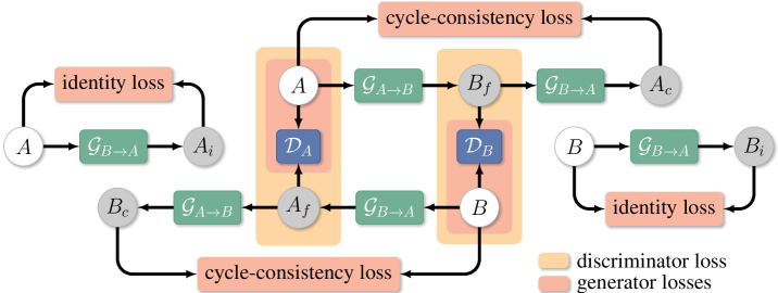
Figure 1: CycleGAN Framework

CycleGAN-like models [82, 42] interlace two generator-discriminator pairs for unpaired image-to-image translation (Figure 1). Denote the two image domains by $A$ and $B$, a CycleGAN-like model uses generator $\mathcal{G}_{A\rightarrow B}$ to translate images from $A$ to $B$, and generator $\mathcal{G}_{B\rightarrow A}$, $B$ to $A$. Discriminator $\mathcal{D}_{A}$ is used to distinguish between images in $A$ and those translated from $B$ (denoted as $A_{f}$ in Figure 1) and discriminator $\mathcal{D}_{B}$, $B$ and $B_{f}$.

The discriminators are updated by backpropagating loss corresponding to failure in distinguishing real and translated images (called generative adversarial loss or GAN loss):

$$\mathcal{L}_{\text{disc},A}= \mathbb{E}_{x\sim{B}}\ell_{\text{GAN}}\left(\mathcal{D}_{A}\left(\mathcal{G}_{B\rightarrow A}(x)\right),0\right)$$

$$+\mathbb{E}_{x\sim{A}}\ell_{\text{GAN}}\left(\mathcal{D}_{A}(x),1\right),$$ (1)

$$\mathcal{L}_{\textrm{disc},B}= \mathbb{E}_{x\sim{A}}\ell_{\text{GAN}}\left(\mathcal{D}_{B}\left(\mathcal{G}_{A\rightarrow B}(x)\right),0\right)$$

$$+\mathbb{E}_{x\sim{B}}\ell_{\text{GAN}}\left(\mathcal{D}_{B}(x),1\right).$$ (2)

Here, $\ell_{\text{GAN}}$ can be any classification loss function ($L_{2}$, cross-entropy, Wasserstein [5], etc.), while the $0$ and $1$ are class labels for translated (fake) and real images, respectively. The generators are updated by backpropagating loss from three sources: GAN loss, cycle-consistency loss, and identity-consistency loss. Using $\mathcal{G}_{A\rightarrow B}$ as an example:

$$\mathcal{L}_{\text{GAN},A}= \mathbb{E}_{x\sim{A}}\ell_{\text{GAN}}\left(\mathcal{D}_{A}\left(\mathcal{G}_{A\rightarrow B}(x)\right),1\right),$$ (3)

$$\mathcal{L}_{\text{cyc},A}= \mathbb{E}_{x\sim{A}}\ell_{\text{reg}}\left(\mathcal{G}_{B\rightarrow A}\left(\mathcal{G}_{A\rightarrow B}(x)\right),x\right),$$ (4)

$$\mathcal{L}_{\text{idt},A}= \mathbb{E}_{x\sim{A}}\ell_{\text{reg}}\left(\mathcal{G}_{B\rightarrow A}\left(x\right),x\right).$$ (5)

And,

$$\mathcal{L}_{\text{gen},A\rightarrow B}= \mathcal{L}_{\text{GAN},A}+\lambda_{\text{cyc}}\mathcal{L}_{\text{cyc},A}+\lambda_{\text{idt}}\mathcal{L}_{\text{idt},A},$$ (6)

$$\mathcal{L}_{\text{gen},B\rightarrow A}= \mathcal{L}_{\text{GAN},B}+\lambda_{\text{cyc}}\mathcal{L}_{\text{cyc},B}+\lambda_{\text{idt}}\mathcal{L}_{\text{idt},B}.$$ (7)

Here, $\ell_{\textrm{reg}}$ can be any regression loss function ($L_{1}$ or $L_{2}$, etc.), and $\lambda_{\text{cyc}}$ and $\lambda_{\text{idt}}$ are combination coefficients.

To improve the original CycleGAN model’s performance, we implement three major changes. First, we modify the generator to have a hybrid architecture based on a UNet with a ViT bottleneck (Section 3.2). Second, to regularize the CycleGAN discriminator, we augment the vanilla CycleGAN discriminator loss with a gradient penalty term (Section 3.3). Finally, instead of training from a randomly initialized network weights, we pre-train generators in a self-supervised fashion on the image inpainting task to obtain a better starting state (Section 3.4).

3.2 UNet-ViT Generator

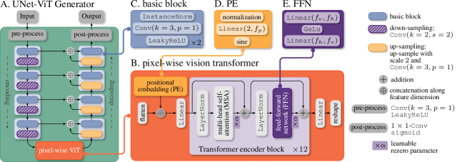
Figure 2: Schematic diagrams of UVCGAN. A. UNet-ViT generator; B. pixel-wise ViT; C. basic block; D. positional embedding (PE); F. feed-forward network (FFN).

A UNet-ViT generator consists of a UNet [67] with a pixel-wise Vision Transformer (ViT) [28] at the bottleneck (Figure 2A). UNet’s encoding path extracts features from the input via four layers of convolution and downsampling. The features extracted at each layer are also passed to the corresponding layers of the decoding path via skip connections, whereas the bottom-most features are passed to the ViT. We hypothesize that the skip connections are effective in passing high-frequency features to the decoder, and the ViT provides an effective means to learn pairwise relationships of low-frequency features.

On the encoding path of the UNet, the pre-processing layer turns an image into a tensor with dimension $(w_{0},h_{0},f_{0})$. A pre-processed tensor will have its width and height halved at each down-sampling block, while the feature dimension doubled at the last three down-sampling blocks. The output from the encoding path with dimension $(w,h,f)=(w_{0}/16,h_{0}/16,8f_{0})$ forms the input to the pixel-wise ViT bottleneck.

A pixel-wise ViT (Figure 2B) is composed primarily of a stack of Transformer encoder blocks [24]. To construct an input to the stack, the ViT first flattens an encoded image along the spatial dimensions to form a sequence of tokens. The token sequence has length $w\times h$, and each token in the sequence is a vector of length $f$. It then concatenates each token with its two-dimensional Fourier positional embedding [4] of dimension $f_{p}$ (Figure 2D) and linearly maps the result to have dimension $f_{v}$. To improve the Transformer convergence, we adopt the rezero regularization [6] scheme and introduce a trainable scaling parameter $\alpha$ that modulates the magnitudes of the nontrivial branches of the residual blocks. The output from the Transformer stack is linearly projected back to have dimension $f$ and unflattened to have width $w$ and $h$. In this study, we use $12$ Transform encoder blocks and set $f,f_{p},f_{v}=384$, and $f_{h}=4f_{v}$ for the feed-forward network in each block (Figure 2E).

3.3 Discriminator Loss with Gradient Penalty (GP)

In this study, we use the least squares GAN (LSGAN) loss function [50] (i.e., $\ell_{\text{GAN}}$ is an $L_{2}$ error) in Eq. (1)-(7) and supplement the discriminator loss with a GP term. GP [34] originally was introduced to be used with Wasserstein GAN (WGAN) loss to ensure the $1$-Lipschitz constraint [5]. However, in our experiments, WGAN $+$ GP yielded overall worse results, which echoes the findings in [51, 52] We have also considered zero-centered GP [52]. In our case, zero-centered GP turned out to be very sensitive to the values of hyperparameters, and did not improve the training stability. Therefore, we settle on a more generic GP form introduced in [40] with the following formula for loss of $\mathcal{D}_{A}$:

$$\mathcal{L}^{\text{GP}}_{\text{disc},A}=\mathcal{L}_{\text{disc},A}+\lambda_{\text{GP}}\mathbb{E}\left[\frac{\left(\|\nabla_{x}\mathcal{D}_{A}(x)\|_{2}-\gamma\right)^{2}}{\gamma^{2}}\right],$$ (8)

where $\mathcal{L}_{\text{disc},A}$ is defined as in Eq. (1), and $\mathcal{L}^{\text{GP}}_{\text{disc},B}$ follows the same form. In our experiments, this $\gamma$-centered GP regularization provides more stable training and less sensitive to the hyperparameter choices. To see the effect of GP on model performance, refer to the ablation study detailed in Section 5.3 and Appendix Section 1.

3.4 Self-Supervised Pre-training by Inpainting

Pre-training is an effective way to prime large networks for downstream tasks [24, 7] that often can bring significant improvement over random initialization. In this work, we pre-train the UVCGAN generators on an image inpainting task. More precisely, we tile images with non-overlapping patches of size $32\times 32$ and mask $40\%$ of the patches by setting their pixel values to zero. The generator is trained to predict the original unmasked image using pixel-wise $L_{1}$ loss. We consider two modes of pre-training: 1) on the same dataset where the subsequent image translation is to be performed and 2) on the ImageNet [23] dataset. In Section 5.3, we conduct an ablation study on these two pre-training modes together with no pre-training.

4 Experiments

4.1 Benchmarking Datasets

To test UVCGAN’s performance, we have completed an extensive literature survey for benchmark datasets. The most popular among them are datasets derived from CelebA [49] and Flickr-Faces [59], as well as the SYNTHIA/GTA-to-Cityscape [68, 18, 65], photo-to-painting [82], Selfie2Anime [42], and animal face datasets [17]. We prioritize our effort on the Selfie2Anime dataset and two others derived from the CelebA dataset: gender swap (denoted as GenderSwap) and adding and removing eyeglasses (marked as Eyeglasses), which have been used in recent papers.

Selfie2Anime [42] is a small dataset with 3.4K images in each domain. Both GenderSwap and Eyeglasses tasks are derived from CelebA [49] based on the gender and eyeglass attributes, respectively. GenderSwap contains about 68K males and 95K females for training, while Eyeglasses includes 11K with glasses and 152K without. For a fair comparison, we do not use CelebA’s validation dataset for training. Instead, we combine it with the test dataset following the convention of [56, 80]. Selfie2Anime contains images of size $256\times 256$ that can be used directly. The CelebA datasets contains images of size $178\times 218$, which we resize and crop to size $256\times 256$ for UVCGAN training.

4.2 UVCGAN Training Procedures

Pre-training. The UVCGAN generators are pre-trained with self-supervised image inpainting. To construct impaired images, we tile images of size $256\times 256$ into non-overlapping $32\times 32$ pixel patches and randomly mask $40\%$ of the patches by zeroing their pixel values. We use the Adam optimizer, cosine annealing learning-rate scheduler, and several standard data augmentations, such as small-angle random rotation, random cropping, random flipping, and color jittering. During pre-training, we do not distinguish the image domains, which means both generators in the ensuing translation training have the same initialization. In this work, we pre-train one generator on ImageNet, another on CelebA, and one on the Selfie2Anime dataset.

Image Translation Training. For all three benchmarking tasks, we train UVCGAN models for one million iterations with a batch size of one. We use the Adam optimizer with the learning rate kept constant at $0.0001$ during the first half of the training then linearly annealed to zero during the second half. We apply three data augmentations: resizing, random cropping, and random horizontal flipping. Before randomly cropping images to $256\times 256$, we enlarge them from $256\times 256$ to $286\times 286$ for Selfie2Anime and $178\times 218$ to $256\times 313$ for CelebA.

Hyperparameter search. The UVCGAN loss functions depend on four hyperparameters: $\lambda_{\text{cyc}}$, $\lambda_{\text{GP}}$, $\lambda_{\text{idt}}$ and $\gamma$, Eq. (6)-(8). If identity loss ($\lambda_{\text{idt}}$) is used, it is always set to $\lambda_{\text{cyc}}/2$ as suggested in [82]. To find the best-performing configuration, we run a small-scale hyperparameter optimization on a grid. Our experiments show that the best performance for all three benchmarking tasks is achieved with the LSGAN $+$ GP with $(\lambda_{\text{GP}}=0.1,\gamma=100)$ and with generators pre-trained on the image translation dataset itself. Optimal $\lambda_{\text{cyc}}$ differs slightly for CelebA and Selfie2Anime at $5$ and $10$, respectively. An ablation study on hyperparameter tuning can be found in Section 5.3. More training details also can be found in the open-source repository [73].

4.3 Other Model Training Details

To fairly represent other models’ performance, we strive to reproduce trained models following three principles. First, if a pre-trained model for a dataset exists, we will use it directly. Second, in the absence of pre-trained models, we will train the model from scratch using a configuration file (if provided), following a description in the original paper, or using a hyperparameter configuration for a similar task. Third, we will keep the source code “as is” unless it absolutely is necessary to make changes. In addition, we have conducted a small-scale hyperparameter tuning on models lacking hyperparameters for certain translation directions (Appendix Sec. 2). Post-processing and evaluation choices also will affect the reported performance (Section 5.2).

ACL-GAN [1] provides configuration file for the GenderSwap dataset. For configuration files for Eyeglasses and Selfie2Anime, we copy the settings for GenderSwap except for the four key parameters $\lambda_{\text{acl}}$, $\lambda_{\text{mask}}$, $\delta_{\text{min}}$, and $\delta_{\text{max}}$, which we modify according to the paper [80, p. 8, Training Details]. Because ACL-GAN does not train two generators jointly, we train a model for each direction for all datasets. Council-GAN [19] provides models for all datasets but only in one direction (selfie to anime, male to female, removing glasses). The pre-tained models output images with size $256$ for GenderSwap and Selfie2Anime and $128$ for Eyeglasses. For a complete comparison, we train models for the missing directions using the same hyperparameters as the existing ones with the exception for Eyeglasses– we train a model for adding glasses for image size $256$. CycleGAN [21] models are trained from scratch with the default settings (resnet_9blocks generators and LSGAN losses, batch size $1$, etc.). Because the original CycleGAN uses square images, we add a pre-processing for CelebA by scaling up the shorter edge to $256$ while maintaining the aspect ratio, followed by a $256\times 256$ random cropping. U-GAT-IT [72] provides the pre-trained model for Selfie2Anime, which is used directly. For the two CelebA datasets, models are trained using default hyperparameters.

Table 1: Training time. CycleGAN, U-GAT-IT, and UVCGAN train two generators jointly. ACL-GAN and Council-GAN’s generators are trained separately for each direction. The time shown is for training both directions.

black!30 Algorithm	black!10Time (hrs)	Jointly Trained	# Para.
ACL-GAN	black!10$\sim 86$		$\sim 55$M
Council-GAN	black!10$\sim 600$		$\sim 116$M
CycleGAN	black!10$\sim 40$	✓	$\sim 28$M
U-GAT-IT	black!10$\sim 140$	✓	$\sim 671$M
UVCGAN	black!10$\sim 60$	✓	$\sim 68$M

Table 1 depicts the training time (in hours) for various models on the CelebA datasets using an NVIDIA RTX A6000 GPU. The times correspond to training the models with a batch size $1$ for one million iterations. U-GAT-IT’s long training time is due to a large number of loss function terms that must be computed, as well as the large size of the generators and discriminators. For Council-GAN, the time stems from training an ensemble of generators, each with its own discriminator, in addition to the domain discriminators. More details are available in the open-source repository [3]

5 Results

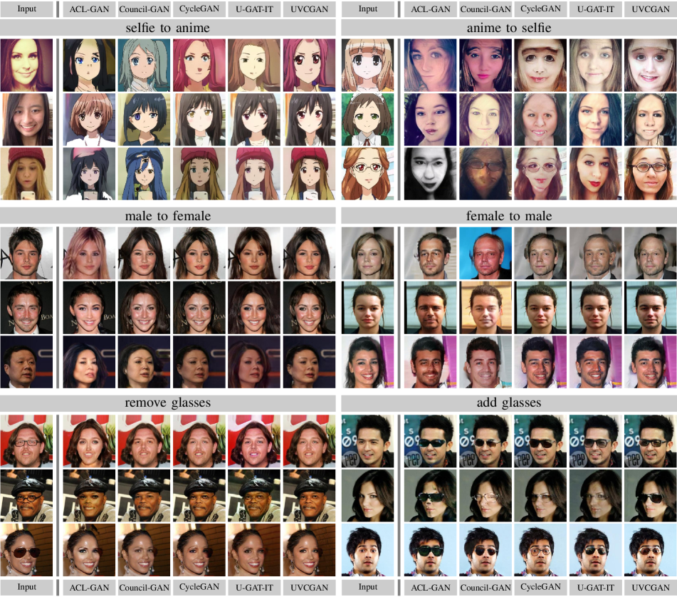
Figure 3: Samples of unpaired image-to-image translation.

5.1 Evaluation Metrics

Fréchet Inception Distance (FID) [36] and Kernel Inception Distance (KID) [10] are the two most accepted metrics used for evaluating image-to-image translation performance. A lower score means the translated images are more similar to those in the target domain. As shown in subsection 5.1, our model offers better performance in most image-to-image translation tasks compared to existing models. As a CycleGAN-like model, ours produce translated images correlated strongly with the input images, such as hair color and face orientations (Figure 3), which is crucial for augmenting scientific simulations. On the contrary, we observed the translations produced by ACL-GAN and Council-GAN tend to be overly liberal on features that are not essential in accomplishing the translation (such as background color or hair color and length). We also note that although U-GAT-IT achieves lower scores in the anime-to-selfie task and produces translations that resemble human faces better, they are less correlated to the input and sometimes miss key features from the input (such as headdress or glasses) that we want to preserve. In the Supplementary material, more samples of larger sizes are provided.

Table 2: FID and KID scores. Lower is better.

black!30black!30	Selfie to Anime		Anime to Selfie
black!30	FID	black!10KID ($\times 100$)	FID	black!10KID ($\times 100$)
black!30ACL-GAN	$99.3$	black!10$3.22\pm 0.26$	$128.6$	black!10$3.49\pm 0.33$
black!30Council-GAN	$91.9$	black!10$2.74\pm 0.26$	$126.0$	black!10$2.57\pm 0.32$
black!30CycleGAN	$92.1$	black!10$2.72\pm 0.29$	$127.5$	black!10$2.52\pm 0.34$
black!30U-GAT-IT	$95.8$	black!10$2.74\pm 0.31$	$\mathbf{108.8}$	black!10$\mathbf{1.48\pm 0.34}$
black!30black!75UVCGAN		black!10$\mathbf{79.0}$	$\mathbf{1.35\pm 0.20}$	black!10$122.8$	$2.33\pm 0.38$
black!30black!75black!30		Male to Female		Female to Male
black!30	FID	black!10KID ($\times 100$)	FID	black!10KID ($\times 100$)
black!30ACL-GAN	$\mathbf{9.4}$	black!10$\mathbf{0.58\pm 0.06}$	$19.1$	black!10$1.38\pm 0.09$
black!30Council-GAN	$10.4$	black!10$0.74\pm 0.08$	$24.1$	black!10$1.79\pm 0.10$
black!30CycleGAN	$15.2$	black!10$1.29\pm 0.11$	$22.2$	black!10$1.74\pm 0.11$
black!30U-GAT-IT	$24.1$	black!10$2.20\pm 0.12$	$15.5$	black!10$0.94\pm 0.07$
black!30black!75UVCGAN		black!10$9.6$	$0.68\pm 0.07$	black!10$\mathbf{13.9}$	$\mathbf{0.91\pm 0.08}$
black!30black!75black!30		Remove Glasses		Add Glasses
black!30	FID	black!10KID ($\times 100$)	FID	black!10KID ($\times 100$)
black!30ACL-GAN	$16.7$	black!10$0.70\pm 0.06$	$20.1$	black!10$1.35\pm 0.14$
black!30Council-GAN	$37.2$	black!10$3.67\pm 0.22$	$19.5$	black!10$1.33\pm 0.13$
black!30CycleGAN	$24.2$	black!10$1.87\pm 0.17$	$19.8$	black!10$1.36\pm 0.12$
black!30U-GAT-IT	$23.3$	black!10$1.69\pm 0.14$	$19.0$	black!10$1.08\pm 0.10$
black!30black!75UVCGAN		black!10$\mathbf{14.4}$	$\mathbf{0.68\pm 0.10}$	black!10$\mathbf{13.6}$	$\mathbf{0.60\pm 0.08}$
black!30black              black!10

5.2 Model Evaluation and Reproducibility

KID and FID for image-to-image translation are difficult to reproduce. For example, in [56, 80, 42], most FID and KID scores of the same task-model settings differ. We hypothesize that this is due to: 1) Different sizes of test data as FID decreases with more data samples [10] 2) Differences in post-processing before testing 3) Different formulation of metrics (e.g. KID in U-GAT-IT [42]) 4) Different FID and KID implementations. Therefore, we standardize the evaluations as follows: 1) Using the full test datasets for FID and KID—for KID subset size, use $50$ for Selfie2Anime and $1000$ for the two CelebA datasets; 2) Resizing non-square CelebA images and taking a central crop of size $256\times 256$ to maintain the correct aspect ratio; 3) Delegating all KID and FID calculations to the torch-fidelity package [60].

ACL-GAN follows a non-deterministic type of cycle consistency and can generate a variable number of translated images for an input. However, because larger sample size improves FID score [10], we generate one translated image per input for a fair comparison. To produce the test result, ACL-GAN resizes images from CelebA to have width $256$ and output without cropping. For FID and KID evaluation, we take the center $256\times 256$ crop from the test output. Council-GAN resizes the images to have a width $256$, except for removing glasses, which is $128$ due to the pre-trained model provided. In order to follow the principle of using a pre-trained model if available and maintain consistency in evaluating on images of size $256$, we resize $128$ to $256$ during testing, which may be responsible for the large FID score. The reverse direction, adding glasses, is trained from scratch using an image size of $256$. Its performance is similar to that of other models. CycleGAN takes a random square crop for both training and testing. However, for a fair comparison, we modify the source code so the test output are the center crops. Since the original U-GAT-IT cannot handle non-square images, we modified the code to scale the shorter edge $256$ for the CelebA datasets.

5.3 Ablation Studies

Table 3 summarizes the male-to-female and selfie-to-anime translation performance with respect to pre-training, GP, and identity loss. First, GP combined with identity loss improves performance. Second, without GP, the identity loss produces mixed results. Finally, pre-training on the same dataset improves performance, especially in conjunction with the GP and identity loss. Appendix Sec. 1 contains the complete ablation study results for all data sets.

We speculate that the GP is required to obtain the best performance with pre-trained networks because those networks provide a good starting point for the image translation task. However, at the beginning of fine-tuning, the discriminator is initialized by random values and provides a meaningless signal to the generator. This random signal may drive the generator away from the good starting point and undermine the benefits of pre-training.

Table 3: Ablation studies. Pre-train/Dataset column indicates which dataset the generator is pre-trained on (None for no pre-training; Same indicates CelebA for male-to-female and Selfie2Anime for selfie-to-anime).

black!30black!30Pre-train			Male to Female		Selfie to Anime
black!30Dataset	GP	idt	FID	black!10KID ($\times 100$)	FID	black!10KID ($\times 100$)
black!30Same	✓	✓	$9.6$	black!10$0.68\pm 0.07$	$79.0$	black!10$1.35\pm 0.20$
black!30ImageNet	✓	✓	$11.0$	black!10$0.85\pm 0.08$	$81.3$	black!10$1.66\pm 0.21$
black!30None	✓	✓	$11.0$	black!10$0.85\pm 0.09$	$80.9$	black!10$1.78\pm 0.20$
black!30Same	✓		$11.1$	black!10$0.86\pm 0.08$	$83.9$	black!10$1.88\pm 0.35$
black!30ImageNet	✓		$11.0$	black!10$0.85\pm 0.08$	$84.3$	black!10$1.77\pm 0.21$
black!30None	✓		$13.4$	black!10$1.11\pm 0.09$	$115.4$	black!10$6.85\pm 0.59$
black!30Same		✓	$14.2$	black!10$1.22\pm 0.10$	$81.5$	black!10$1.68\pm 0.22$
black!30ImageNet		✓	$14.5$	black!10$1.23\pm 0.10$	$86.8$	black!10$2.21\pm 0.25$
black!30None		✓	$14.4$	black!10$1.26\pm 0.10$	$81.6$	black!10$1.75\pm 0.25$
black!30Same			$12.7$	black!10$1.06\pm 0.09$	$79.0$	black!10$1.32\pm 0.19$
black!30ImageNet			$13.4$	black!10$1.14\pm 0.10$	$91.2$	black!10$2.63\pm 0.23$
black!30None			$18.3$	black!10$1.63\pm 0.11$	$81.2$	black!10$1.76\pm 0.21$

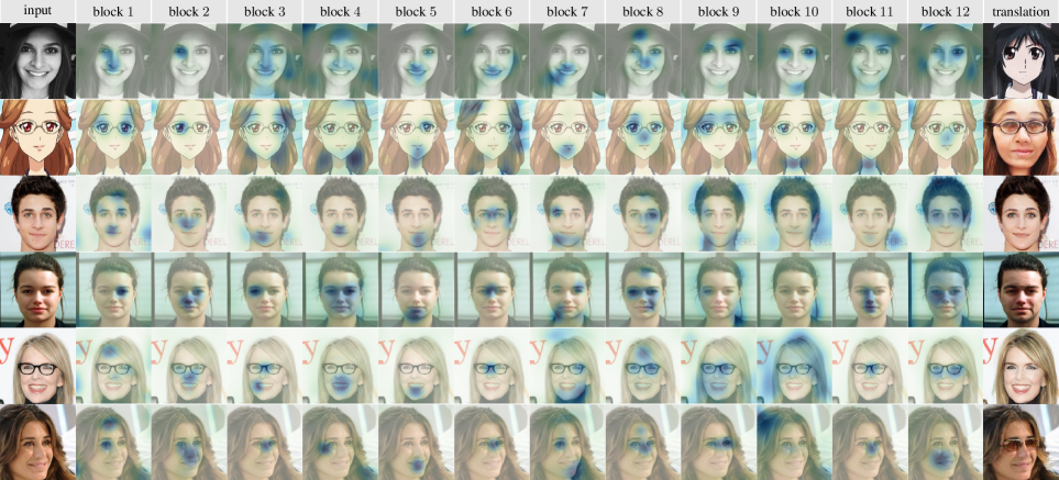
Figure 4: Attention. Attention heatmap generated by the attention weights from the 12 Transformer encoder blocks in the pixel-wise ViT. The attention heatmap demonstrates the amount of attention different locations of an image receive.

5.4 Interpretation of Attention

Because the UVCGAN generator uses the transformer bottleneck, it is instructive to visualize its attention matrices to see if they help with generator interpretability. We plot (Figure 4) the attention weights produced by the multi-head self-attention (MSA) unit in each of the $12$ Transformer encoder blocks in the bottleneck of the UVCGAN generators (Figure 2B). The $(i,j)$-entry of the attention matrix indicates how much attention token $i$ is paying to token $j$ while the sum of row $i$ is one. When multi-head attention is used, each head produces an attention matrix. For simplicity, we average the attention weights over all heads and target tokens for each block in the Transformer encoder stack. Given the input image of size $256\times 256$, this provides an attention vector of dimension $w\times h$ ($16\times 16=256$). The $j$-th entry of such a vector indicates how much attention token $j$ receives on average. Because the tokens represent overlapping patches in the original image, we generate a heatmap as follows: reshape a feature vector to a square of size $16\times 16$, upscale it 16 folds to match the dimension of the input image, then apply a Gaussian filter with $\sigma=16$. By overlaying the attention heatmap on the input images, we note that each block is paying attention to a specific facial part with the eye and mouth areas receiving the most attention. This echoes the findings in behavioral science experiments on statistical eye fixation (e.g.,  [12]), where the regions of interest also tend to be around the eyes and mouth, which may indicate that the model’s attention is focused on the most informative and relevant regions.

6 Conclusion

This work introduces UVCGAN to promote cycle-consistent, content-preserving image translation and effectively handle long-range spatial dependencies that remain a common problem in scientific domain research. Combined with self-supervised pre-training and GP regularization, UVCGAN outperforms competing methods on a diverse set of image translation benchmarks. The ablation study suggests GP and cycle-consistent loss work well with UVCGAN. Additional inspection on attention weights indicates our model has focused on the relevant regions of the source images. To further demonstrate the effectiveness of our model in handling long-distance patterns beyond benchmark datasets, more open scientific datasets are needed.

Potential Negative Social Impact. All data used in this work are publicly available. The environmental impact of training our model is greater than the original CycleGAN yet considerably less comparing to other advanced models. Although the motivation of our image-to-image translation work is to bridge the gap between scientific simulation and experiment, the authors are aware of its potential use for generating fake content [53]. Thankfully, there are countermeasures and detection tools [39] developed to counter such misuse. To contribute to such mitigation efforts, we have made our code and pre-trained models available.

Acknowledgement. The LDRD Program at Brookhaven National Laboratory, sponsored by DOE’s Office of Science under Contract DE-SC0012704, supported this work.

Appendix A Extended UVCGAN Ablation Studies

This appendix shows the impact of the UVCGAN generator, gradient penalty (GP), and self-supervised generator pretraining (PT) on UVCGAN’s performance. Appendix A summarizes these findings. For each data set, the bottom half of the table shows the UVCGAN performance with some of its components disabled. For example, UVCGAN no GP shows the UVCGAN performance without the gradient penalty term (but using a hybrid UNet-ViT generator and a self-supervised pretraining). This table affords a few observations: 1. the addition of a hybrid UNet-ViT generator alone typically produces a large degree of improvement compared to CycleGAN, even in the absence of the self-supervised pre-training and GP term; 2. the self-supervised generator pre-training without the GP term does not seem to improve the image-to-image translation performance and sometimes makes it worse; 3. the self-supervised pre-training only helps when it is used in conjunction with the GP.

Table A1: FID and KID scores. Lower is better. PT stands for the self-supervised generator pre-training, and GP means usage of the gradient penalty.

black!30black!30	Selfie to Anime		Anime to Selfie
black!30	FID	black!10KID ($\times 100$)	FID	black!10KID ($\times 100$)
black!30ACL-GAN	$99.3$	black!10$3.22\pm 0.26$	$128.6$	black!10$3.49\pm 0.33$
black!30Council-GAN	$91.9$	black!10$2.74\pm 0.26$	$126.0$	black!10$2.57\pm 0.32$
black!30CycleGAN	$92.1$	black!10$2.74\pm 0.31$	$127.5$	black!10$2.52\pm 0.34$
black!30U-GAT-IT	$95.8$	black!10$2.74\pm 0.31$	$\mathbf{108.8}$	black!10$\mathbf{1.48\pm 0.34}$
black!30black!75UVCGAN		black!10$\mathbf{79.0}$	$\mathbf{1.35\pm 0.20}$	black!10$122.8$	$2.33\pm 0.38$
black!30UVCGAN no GP	$81.4$	black!10$1.68\pm 0.22$	$133.3$	black!10$2.90\pm 0.49$
black!30UVCGAN no PT	$80.9$	black!10$1.78\pm 0.20$	$134.0$	black!10$2.98\pm 0.49$
black!30UVCGAN no PT and GP	$81.6$	black!10$1.75\pm 0.25$	$140.6$	black!10$3.53\pm 0.59$
black!30black!75black!30		Male to Female		Female to Male
black!30	FID	black!10KID ($\times 100$)	FID	black!10KID ($\times 100$)
black!30ACL-GAN	$\mathbf{9.4}$	black!10$\mathbf{0.58\pm 0.06}$	$19.1$	black!10$1.38\pm 0.09$
black!30Council-GAN	$10.4$	black!10$0.74\pm 0.08$	$24.1$	black!10$1.79\pm 0.10$
black!30CycleGAN	$15.2$	black!10$1.29\pm 0.11$	$22.2$	black!10$1.74\pm 0.11$
black!30U-GAT-IT	$24.1$	black!10$2.20\pm 0.12$	$15.5$	black!10$0.94\pm 0.07$
black!30black!75UVCGAN		black!10$9.6$	$0.68\pm 0.07$	black!10$\mathbf{13.9}$	$\mathbf{0.91\pm 0.08}$
black!30UVCGAN no GP	$14.1$	black!10$1.22\pm 0.10$	$20.4$	black!10$1.61\pm 0.11$
black!30UVCGAN no PT	$11.0$	black!10$0.85\pm 0.09$	$14.7$	black!10$0.98\pm 0.08$
black!30UVCGAN no PT and GP	$14.4$	black!10$1.26\pm 0.10$	$19.9$	black!10$1.55\pm 0.11$
black!30black!75black!30		Remove Glasses		Add Glasses
black!30	FID	black!10KID ($\times 100$)	FID	black!10KID ($\times 100$)
black!30ACL-GAN	$16.7$	black!10$0.70\pm 0.06$	$20.1$	black!10$1.35\pm 0.14$
black!30Council-GAN	$37.2$	black!10$3.67\pm 0.22$	$19.5$	black!10$1.33\pm 0.13$
black!30CycleGAN	$24.2$	black!10$1.87\pm 0.17$	$19.8$	black!10$1.36\pm 0.12$
black!30U-GAT-IT	$23.3$	black!10$1.69\pm 0.14$	$19.0$	black!10$1.08\pm 0.10$
black!30black!75UVCGAN		black!10$\mathbf{14.4}$	$\mathbf{0.68\pm 0.10}$	black!10$\mathbf{13.6}$	$\mathbf{0.60\pm 0.08}$
black!30UVCGAN no GP	$19.2$	black!10$1.28\pm 0.15$	$18.7$	black!10$1.14\pm 0.12$
black!30UVCGAN no PT	$15.8$	black!10$0.84\pm 0.12$	$14.3$	black!10$0.70\pm 0.10$
black!30UVCGAN no PT and GP	$19.7$	black!10$1.32\pm 0.15$	$16.1$	black!10$0.89\pm 0.11$
black!30black              black!10

Appendix B Hyperparameter Tuning for Other Algorithms

This section summarizes the hyperparameter tuning results for three benchmarking algorithms: ACL-GAN, CycleGAN, and U-GAT-IT. We omitted tuning for Council-GAN because it takes too long to run ($300$ hours per translation).

Because none of the benchmarking algorithms use any stablization techniques (such as the EMA of network weight [41]) beyond shrinking learning rate, we suspect the fluctuation may be at least partially due to instability of the GAN training.

We only provide hyperparameter tuning results for a data set or task if an algorithm did not work on it. We skip hyperparameter tuning if either a pre-trained model or a hyperparameter setup was provided by the author. In Table A2-A4, the best results are marked in bold font. The default hyperparameters are highlighted in gray.

ACL-GAN worked on all three data sets studied and detailed in this paper—but all for only one direction: selfie-to-anime, male-to-female, and remove glasses. For the translation in the opposite directions, we tune three parameters concerning the focus loss: focus loss weight, focus upper, and focus lower. The results are summarized in Table A2.

Table A2: ACL-GAN hyperparameter tuning results. We tune three hyperparameters related to the focus loss: weight of the focus loss, focus upper, and focus lower.

task	weight	upper	lower	FID	KID($\times 100$)
anime-to-selfie	black!20$0$	black!20$-$	black!20$-$	black!20$\mathbf{128.6}$	black!20$\mathbf{3.49\pm 0.33}$
	$.025$	$.5$	$.3$	$205.3$	$11.0\pm 1.01$
	$.025$	$.1$	$.05$	$250.3$	$18.6\pm 1.19$
female-to-male	$0$	$-$	$-$	$46.0$	$3.39\pm 0.13$
	black!20$.025$	black!20$.5$	black!20$.3$	black!20$\mathbf{19.1}$	black!20$\mathbf{1.38\pm 0.09}$
	$.05$	$.5$	$.3$	$36.3$	$2.91\pm 0.13$
add glasses	$0$	$-$	$-$	$29.0$	$1.77\pm 0.12$
	black!20$.025$	black!20$.1$	black!20$.05$	black!20$26.6$	black!20$2.26\pm 0.17$
	$.05$	$.1$	$.05$	$\mathbf{20.1}$	$\mathbf{1.35\pm 0.14}$

CycleGAN did not work on any of the three data sets. We search a grid on two hyperparameters: type of generator (Gen.) and weight (Wt.) of cycle-consistency loss. We also try two GAN modes: lsgan and wgangp. However, because CycleGAN did not implement GP properly, wgangp did not work. The results are summarized in Table A3.

Table A3: CycGAN hyperparameter tuning results.

		FID	KID($\times 100$)	FID	KID($\times 100$)
gen.	Wt.	selfie-to-anime		anime-to-selfie
ResNet	$5$	$\mathbf{92.1}$	$\mathbf{2.72\pm 0.29}$	$\mathbf{127.5}$	$\mathbf{2.52\pm 0.34}$
black!20 ResNet	$10$	$93.4$	$2.96\pm 0.27$	$129.4$	$2.91\pm 0.39$
UNet	$5$	$121.9$	$6.21\pm 0.32$	$134.3$	$2.96\pm 0.30$
UNet	$10$	$286.0$	$27.0\pm 0.87$	$135.8$	$3.32\pm 0.32$
		male-to-female		female-to-male
ResNet	$5$	$21.9$	$2.00\pm 0.12$	$33.6$	$2.82\pm 0.14$
black!20 ResNet	$10$	$\mathbf{15.2}$	$\mathbf{1.29\pm 0.11}$	$\mathbf{22.2}$	$\mathbf{1.74\pm 0.11}$
UNet	$5$	$45.5$	$4.55\pm 0.17$	$50.8$	$4.86\pm 0.16$
UNet	$10$	$47.4$	$4.82\pm 0.19$	$47.5$	$4.57\pm 0.17$
		remove glasses		add glasses
ResNet	$5$	$27.7$	$2.08\pm 0.16$	$26.0$	$1.77\pm 0.11$
black!20 ResNet	$10$	$\mathbf{24.2}$	$\mathbf{1.87\pm 0.17}$	$\mathbf{19.8}$	$\mathbf{1.36\pm 0.12}$
UNet	$5$	$32.2$	$2.52\pm 0.19$	$37.3$	$2.90\pm 0.14$
UNet	$10$	$32.2$	$2.52\pm 0.19$	$44.9$	$3.63\pm 0.20$

In addition to hyperparameter tuning for U-GAT-IT, we also correct the aspect ratio problem of U-GAT-IT in this revised version as the original U-GAT-IT implementation cannot handle images with different height and width. We implement the rescaling in the preprocessing stage, so a CelebA image of width $178$ and height $218$ is resized to have width $256$ and height $313$. As we did for CycleGAN and UVCGAN, we take a random $256\times 256$ crop from a training image and a central $256\times 256$ crop from a test image.

U-GAT-IT studied the selfie-to-anime data set. For the two CelebA data sets, we try three levels of weight of cycle-consistency loss: $(5,10,\text{and }20)$ and summarize the results in Table A4.

Table A4: U-GAT-IT hyperparameter tuning results.

	FID	KID($\times 100$)	FID	KID($\times 100$)
weight	male-to-female		female-to-male
$5$	$39.2$	$3.86\pm 0.15$	$45.1$	$4.04\pm 0.16$
black!20 $10$	$\mathbf{24.1}$	$\mathbf{2.20\pm 0.12}$	$\mathbf{15.5}$	$\mathbf{0.94\pm 0.07}$
$20$	$32.1$	$3.09\pm 0.16$	$47.5$	$4.42\pm 0.17$
	remove glasses		add glasses
$5$	$34.9$	$2.63\pm 0.15$	$50.0$	$5.08\pm 0.26$
black!20 $10$	$\mathbf{23.3}$	$\mathbf{1.69\pm 0.14}$	$\mathbf{19.0}$	$\mathbf{1.08\pm 0.10}$
$20$	$36.1$	$3.13\pm 0.19$	$36.1$	$2.67\pm 0.13$

Appendix C More detail about the UNet-ViT Generator

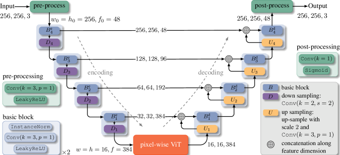
Figure A1: UNet ViT Generator with Full Details

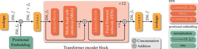
Figure A2: Vision Transformer with Full Details

A UNet-ViT generator consists of a UNet [67] with a pixel-wise Vision Transformer (ViT) [28] at the bottleneck (Figure A1). UNet’s encoding path extracts features from the input via four layers of convolution and downsampling. The features extracted at each layer are also passed to the corresponding layers of the decoding path via the skip connections, whereas the bottom-most features are passed to the pixel-wise ViT (Figure A2).

On UNet’s encoding path, the pre-processing layer turns an image into a tensor with dimension $(w_{0},h_{0},f_{0})$. Each layer of the encoding path consists of a basic and downsampling block. The basic block is composed primarily of two convolutions, while the downsampling block has one convolution with stride $2$. A pre-processed tensor will have its width and height halved at each downsampling block, while the feature dimension doubles at the last three downsampling blocks. Hence, the output from the encoding path will have dimension $(w,h,f)=(w_{0}/16,h_{0}/16,8f_{0})$, and it forms the input to the pixel-wise ViT bottleneck. Each layer of the UNet decoding path consists of an upsampling block followed by a basic block. A basic block on the decoding path differs from one on the encoding path in that it takes as input a concatenated tensor as input formed with the output from the upsampling layer and the tensor from the corresponding skip connection of the encoding path. The decoding path’s output will go through a post-processing layer of $1\times 1$ convolution with a sigmoid activation to produce an image.

A pixel-wise ViT is composed primarily of a stack of Transformer encoder blocks [24]. To construct an input to the stack, the ViT first flattens an encoding along the spatial dimensions to form a sequence of transformer tokens. The token sequence has length $w\times h$, and each token in the sequence is a vector of length $f$. It then concatenates each token with its two-dimensional Fourier positional embedding [4] of dimension $f_{p}$ and linearly maps the result to have dimension $f_{v}$. To improve the Transformer convergence, we adopt the rezero regularization [6] scheme and introduce a trainable scaling parameter $\alpha$ that modulates the magnitudes of the nontrivial branches of the residual blocks. The Transformer stack output is linearly projected back to have dimension $f$ and unflattened to have width $w$ and $h$. In this study, we use input raw or cropped images with $w_{0}=h_{0}=256$ and set $f_{0}=48$. Hence, we have $w=h=16$ and $f=384$. We use $12$ Transform encoder blocks in ViT and set $f_{p},f_{v}=f$, and $f_{h}=4f_{v}$ for the feed-forward network in each transformer encoder block.

Appendix D Additional Sample Translations

We show a few more translations in Figures A3 to A5.

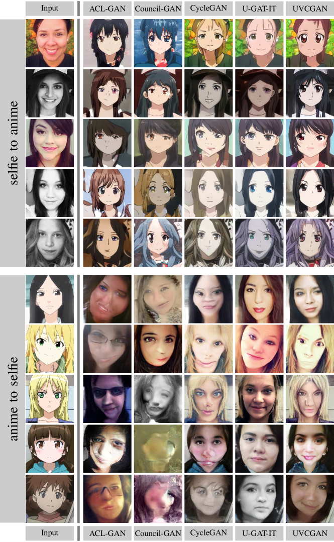
Figure A3: Additional Sample Translations: Selfie2Anime

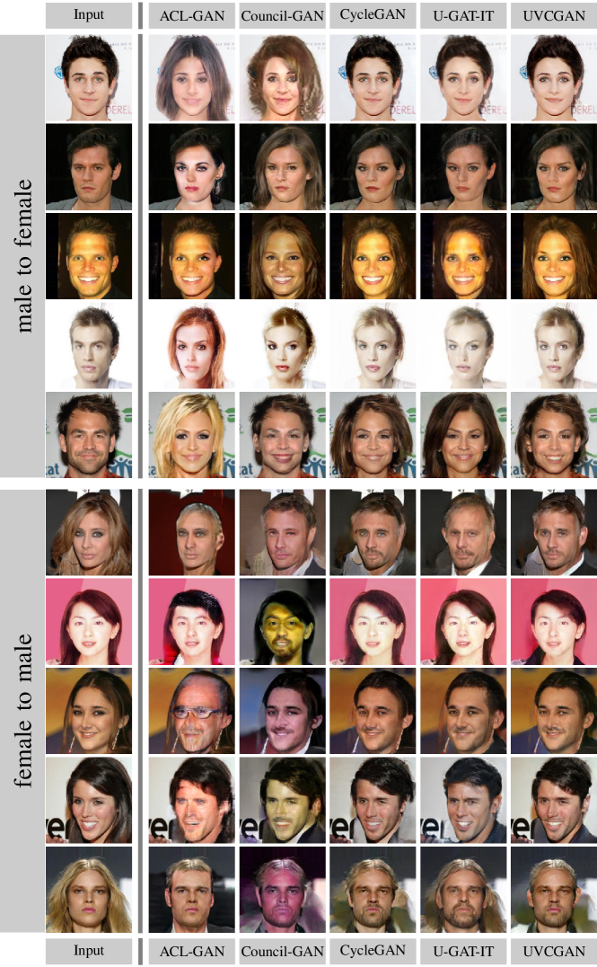
Figure A4: Additional Sample Translations: GenderSwap

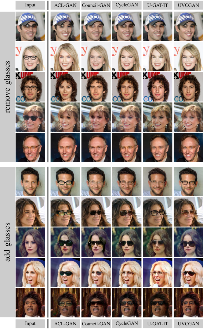
Figure A5: Additional Sample Translations: Eyeglasses

References

- [1] GitHub: ACL-GAN. https://github.com/hyperplane-lab/acl-gan.
- [2] Yasir Alanazi, Nobuo Sato, Tianbo Liu, Wally Melnitchouk, Pawel Ambrozewicz, Florian Hauenstein, Michelle P. Kuchera, Evan Pritchard, Michael Robertson, Ryan Strauss, Luisa Velasco, and Yaohang Li. Simulation of electron-proton scattering events by a feature-augmented and transformed generative adversarial network (FAT-GAN). In Zhi-Hua Zhou, editor, Proceedings of the Thirtieth International Joint Conference on Artificial Intelligence, IJCAI-21, pages 2126–2132. International Joint Conferences on Artificial Intelligence Organization.
- [3] GitHub: UVCGAN-Benchmarking Algorithms. https://github.com/ls4gan/benchmarking.
- [4] Ivan Anokhin, Kirill Demochkin, Taras Khakhulin, Gleb Sterkin, Victor Lempitsky, and Denis Korzhenkov. Image generators with conditionally-independent pixel synthesis. In Proceedings of the IEEE/CVF Conference on Computer Vision and Pattern Recognition, pages 14278–14287, 2021.
- [5] Martin Arjovsky, Soumith Chintala, and Léon Bottou. Wasserstein generative adversarial networks. In International conference on machine learning, pages 214–223. PMLR, 2017.
- [6] Thomas Bachlechner, Bodhisattwa Prasad Majumder, Henry Mao, Gary Cottrell, and Julian McAuley. Rezero is all you need: Fast convergence at large depth. In Uncertainty in Artificial Intelligence, pages 1352–1361. PMLR, 2021.
- [7] Hangbo Bao, Li Dong, and Furu Wei. Beit: Bert pre-training of image transformers. arXiv preprint arXiv:2106.08254, 2021.
- [8] Irwan Bello, William Fedus, Xianzhi Du, Ekin Dogus Cubuk, Aravind Srinivas, Tsung-Yi Lin, Jonathon Shlens, and Barret Zoph. Revisiting resnets: Improved training and scaling strategies. Advances in Neural Information Processing Systems, 34:22614–22627, 2021.
- [9] Camille Bilodeau, Wengong Jin, Tommi Jaakkola, Regina Barzilay, and Klavs F. Jensen. Generative models for molecular discovery: Recent advances and challenges. n/a:e1608. _eprint: https://onlinelibrary.wiley.com/doi/pdf/10.1002/wcms.1608.
- [10] Mikołaj Bińkowski, Danica J Sutherland, Michael Arbel, and Arthur Gretton. Demystifying mmd gans. arXiv preprint arXiv:1801.01401, 2018.
- [11] Andrew Brock, Jeff Donahue, and Karen Simonyan. Large scale GAN training for high fidelity natural image synthesis.
- [12] Roberto Caldara and Sébastien Miellet. imap: a novel method for statistical fixation mapping of eye movement data. Behavior research methods, 43(3):864–878, 2011.
- [13] Mathilde Caron, Hugo Touvron, Ishan Misra, Hervé Jégou, Julien Mairal, Piotr Bojanowski, and Armand Joulin. Emerging properties in self-supervised vision transformers. In Proceedings of the IEEE/CVF International Conference on Computer Vision, pages 9650–9660, 2021.
- [14] Ricky T. Q. Chen, Jens Behrmann, David Duvenaud, and Jörn-Henrik Jacobsen. Residual flows for invertible generative modeling. In Proceedings of the 33rd International Conference on Neural Information Processing Systems. Curran Associates Inc.
- [15] Ting Chen, Simon Kornblith, Mohammad Norouzi, and Geoffrey Hinton. A simple framework for contrastive learning of visual representations. In International conference on machine learning, pages 1597–1607. PMLR.
- [16] Xinlei Chen and Kaiming He. Exploring simple siamese representation learning. In Proceedings of the IEEE/CVF Conference on Computer Vision and Pattern Recognition, pages 15750–15758.
- [17] Yunjey Choi, Youngjung Uh, Jaejun Yoo, and Jung-Woo Ha. Stargan v2: Diverse image synthesis for multiple domains. In Proceedings of the IEEE Conference on Computer Vision and Pattern Recognition, 2020.
- [18] Marius Cordts, Mohamed Omran, Sebastian Ramos, Timo Rehfeld, Markus Enzweiler, Rodrigo Benenson, Uwe Franke, Stefan Roth, and Bernt Schiele. The cityscapes dataset for semantic urban scene understanding. In Proceedings of the IEEE conference on computer vision and pattern recognition, pages 3213–3223, 2016.
- [19] GitHub: Council-GAN. https://github.com/onr/council-gan.
- [20] Kyle Cranmer, Johann Brehmer, and Gilles Louppe. The frontier of simulation-based inference. Proceedings of the National Academy of Sciences, 117(48):30055–30062, 2020. Publisher: National Academy of Sciences Section: Colloquium Paper.
- [21] GitHub: CycleGAN. https://github.com/junyanz/pytorch-cyclegan-and-pix2pix.
- [22] Payel Das, Tom Sercu, Kahini Wadhawan, Inkit Padhi, Sebastian Gehrmann, Flaviu Cipcigan, Vijil Chenthamarakshan, Hendrik Strobelt, Cicero dos Santos, Pin-Yu Chen, Yi Yan Yang, Jeremy P. K. Tan, James Hedrick, Jason Crain, and Aleksandra Mojsilovic. Accelerated antimicrobial discovery via deep generative models and molecular dynamics simulations. 5(6):613–623. Number: 6 Publisher: Nature Publishing Group.
- [23] Jia Deng, Wei Dong, Richard Socher, Li-Jia Li, Kai Li, and Li Fei-Fei. Imagenet: A large-scale hierarchical image database. In 2009 IEEE Conference on Computer Vision and Pattern Recognition, pages 248–255, 2009.
- [24] Jacob Devlin, Ming-Wei Chang, Kenton Lee, and Kristina Toutanova. Bert: Pre-training of deep bidirectional transformers for language understanding, 2019.
- [25] Riccardo Di Sipio, Michele Faucci Giannelli, Sana Ketabchi Haghighat, and Serena Palazzo. DijetGAN: a generative-adversarial network approach for the simulation of QCD dijet events at the LHC. 2019(8):110.
- [26] Laurent Dinh, Jascha Sohl-Dickstein, and Samy Bengio. Density estimation using real NVP.
- [27] C. Doersch and A. Zisserman. Multi-task self-supervised visual learning. In 2017 IEEE International Conference on Computer Vision (ICCV), pages 2070–2079. IEEE Computer Society. ISSN: 2380-7504.
- [28] Alexey Dosovitskiy, Lucas Beyer, Alexander Kolesnikov, Dirk Weissenborn, Xiaohua Zhai, Thomas Unterthiner, Mostafa Dehghani, Matthias Minderer, Georg Heigold, Sylvain Gelly, et al. An image is worth 16x16 words: Transformers for image recognition at scale. arXiv preprint arXiv:2010.11929, 2020.
- [29] Addis S. Fuhr and Bobby G. Sumpter. Deep generative models for materials discovery and machine learning-accelerated innovation. 9.
- [30] Ian Goodfellow, Jean Pouget-Abadie, Mehdi Mirza, Bing Xu, David Warde-Farley, Sherjil Ozair, Aaron Courville, and Yoshua Bengio. Generative adversarial nets. In Z. Ghahramani, M. Welling, C. Cortes, N. Lawrence, and K. Q. Weinberger, editors, Advances in Neural Information Processing Systems, volume 27. Curran Associates, Inc., 2014.
- [31] Will Grathwohl, Ricky T. Q. Chen, Jesse Bettencourt, Ilya Sutskever, and David Duvenaud. FFJORD: Free-form continuous dynamics for scalable reversible generative models.
- [32] Timofey Grigoryev, Andrey Voynov, and Artem Babenko. When, why, and which pretrained GANs are useful? In International Conference on Learning Representations.
- [33] Jean-Bastien Grill, Florian Strub, Florent Altché, Corentin Tallec, Pierre Richemond, Elena Buchatskaya, Carl Doersch, Bernardo Avila Pires, Zhaohan Guo, Mohammad Gheshlaghi Azar, et al. Bootstrap your own latent-a new approach to self-supervised learning. Advances in neural information processing systems, 33:21271–21284, 2020.
- [34] Ishaan Gulrajani, Faruk Ahmed, Martin Arjovsky, Vincent Dumoulin, and Aaron Courville. Improved training of wasserstein gans, 2017.
- [35] Jianyuan Guo, Kai Han, Han Wu, Chang Xu, Yehui Tang, Chunjing Xu, and Yunhe Wang. Cmt: Convolutional neural networks meet vision transformers. arXiv preprint arXiv:2107.06263, 2021.
- [36] Martin Heusel, Hubert Ramsauer, Thomas Unterthiner, Bernhard Nessler, and Sepp Hochreiter. Gans trained by a two time-scale update rule converge to a local nash equilibrium. In I. Guyon, U. V. Luxburg, S. Bengio, H. Wallach, R. Fergus, S. Vishwanathan, and R. Garnett, editors, Advances in Neural Information Processing Systems, volume 30. Curran Associates, Inc., 2017.
- [37] Jonathan Ho, Ajay Jain, and Pieter Abbeel. Denoising diffusion probabilistic models. type: article.
- [38] Xun Huang, Ming-Yu Liu, Serge Belongie, and Jan Kautz. Multimodal unsupervised image-to-image translation. In Proceedings of the European conference on computer vision (ECCV), pages 172–189, 2018.
- [39] Felix Juefei-Xu, Run Wang, Yihao Huang, Qing Guo, Lei Ma, and Yang Liu. Countering malicious deepfakes: Survey, battleground, and horizon. International Journal of Computer Vision, pages 1–57, 2022.
- [40] Tero Karras, Timo Aila, Samuli Laine, and Jaakko Lehtinen. Progressive growing of GANs for improved quality, stability, and variation.
- [41] Tero Karras, Samuli Laine, Miika Aittala, Janne Hellsten, Jaakko Lehtinen, and Timo Aila. Analyzing and improving the image quality of stylegan. In Proceedings of the IEEE/CVF conference on computer vision and pattern recognition, pages 8110–8119, 2020.
- [42] Junho Kim, Minjae Kim, Hyeonwoo Kang, and Kwang Hee Lee. U-gat-it: Unsupervised generative attentional networks with adaptive layer-instance normalization for image-to-image translation. In International Conference on Learning Representations, 2019.
- [43] Durk P Kingma and Prafulla Dhariwal. Glow: Generative flow with invertible 1x1 convolutions. In S. Bengio, H. Wallach, H. Larochelle, K. Grauman, N. Cesa-Bianchi, and R. Garnett, editors, Advances in Neural Information Processing Systems, volume 31. Curran Associates, Inc.
- [44] Diederik P Kingma and Max Welling. Auto-encoding variational bayes.
- [45] Diederik P. Kingma and Max Welling. An introduction to variational autoencoders. 12(4):307–392.
- [46] Nikos Komodakis and Spyros Gidaris. Unsupervised representation learning by predicting image rotations. In International Conference on Learning Representations (ICLR).
- [47] Hsin-Ying Lee, Hung-Yu Tseng, Jia-Bin Huang, Maneesh Singh, and Ming-Hsuan Yang. Diverse image-to-image translation via disentangled representations. In Proceedings of the European conference on computer vision (ECCV), pages 35–51, 2018.
- [48] Qi Liu, Miltiadis Allamanis, Marc Brockschmidt, and Alexander L. Gaunt. Constrained graph variational autoencoders for molecule design. In Proceedings of the 32nd International Conference on Neural Information Processing Systems, NIPS’18, pages 7806–7815. Curran Associates Inc. event-place: Montréal, Canada.
- [49] Ziwei Liu, Ping Luo, Xiaogang Wang, and Xiaoou Tang. Deep learning face attributes in the wild. In Proceedings of International Conference on Computer Vision (ICCV), December 2015.
- [50] Xudong Mao, Qing Li, Haoran Xie, Raymond YK Lau, Zhen Wang, and Stephen Paul Smolley. Least squares generative adversarial networks. In Proceedings of the IEEE international conference on computer vision, pages 2794–2802, 2017.
- [51] Xudong Mao, Qing Li, Haoran Xie, Raymond Y.K. Lau, Zhen Wang, and Stephen Paul Smolley. On the effectiveness of least squares generative adversarial networks. IEEE Transactions on Pattern Analysis and Machine Intelligence, 41(12):2947–2960, 2019.
- [52] Lars Mescheder, Andreas Geiger, and Sebastian Nowozin. Which training methods for gans do actually converge? In International conference on machine learning, pages 3481–3490. PMLR, 2018.
- [53] Yisroel Mirsky and Wenke Lee. The creation and detection of deepfakes: A survey. ACM Computing Surveys (CSUR), 54(1):1–41, 2021.
- [54] Mustafa Mustafa, Deborah Bard, Wahid Bhimji, Zarija Lukić, Rami Al-Rfou, and Jan M. Kratochvil. CosmoGAN: creating high-fidelity weak lensing convergence maps using generative adversarial networks. 6(1):1.
- [55] Alex Nichol, Prafulla Dhariwal, Aditya Ramesh, Pranav Shyam, Pamela Mishkin, Bob McGrew, Ilya Sutskever, and Mark Chen. GLIDE: Towards photorealistic image generation and editing with text-guided diffusion models. type: article.
- [56] Ori Nizan and Ayellet Tal. Breaking the cycle–colleagues are all you need. In 2020 IEEE/CVF Conference on Computer Vision and Pattern Recognition (CVPR), pages 7857–7866. IEEE, 2020.
- [57] Atsuhiro Noguchi and Tatsuya Harada. Image generation from small datasets via batch statistics adaptation. In Proceedings of the IEEE/CVF International Conference on Computer Vision, pages 2750–2758.
- [58] Mehdi Noroozi and Paolo Favaro. Unsupervised learning of visual representations by solving jigsaw puzzles. In European conference on computer vision, pages 69–84. Springer.
- [59] NVlabs/ffhq dataset. https://github.com/nvlabs/ffhq-dataset.
- [60] Anton Obukhov, Maximilian Seitzer, Po-Wei Wu, Semen Zhydenko, Jonathan Kyl, and Elvis Yu-Jing Lin. High-fidelity performance metrics for generative models in pytorch, 2020. Version: 0.3.0, DOI: 10.5281/zenodo.4957738.
- [61] Taesung Park, Alexei A Efros, Richard Zhang, and Jun-Yan Zhu. Contrastive learning for unpaired image-to-image translation. In European conference on computer vision, pages 319–345. Springer.
- [62] Deepak Pathak, Philipp Krahenbuhl, Jeff Donahue, Trevor Darrell, and Alexei A Efros. Context encoders: Feature learning by inpainting. In Proceedings of the IEEE conference on computer vision and pattern recognition, pages 2536–2544.
- [63] Alec Radford, Karthik Narasimhan, Tim Salimans, Ilya Sutskever, et al. Improving language understanding by generative pre-training. 2018.
- [64] Ali Razavi, Aaron Van den Oord, and Oriol Vinyals. Generating diverse high-fidelity images with vq-vae-2. 32.
- [65] Stephan R Richter, Vibhav Vineet, Stefan Roth, and Vladlen Koltun. Playing for data: Ground truth from computer games. In European conference on computer vision, pages 102–118. Springer, 2016.
- [66] Robin Rombach, Andreas Blattmann, Dominik Lorenz, Patrick Esser, and Björn Ommer. High-resolution image synthesis with latent diffusion models. type: article.
- [67] Olaf Ronneberger, Philipp Fischer, and Thomas Brox. U-net: Convolutional networks for biomedical image segmentation. In International Conference on Medical image computing and computer-assisted intervention, pages 234–241. Springer, 2015.
- [68] German Ros, Laura Sellart, Joanna Materzynska, David Vazquez, and Antonio M Lopez. The synthia dataset: A large collection of synthetic images for semantic segmentation of urban scenes. In Proceedings of the IEEE conference on computer vision and pattern recognition, pages 3234–3243, 2016.
- [69] Tim Salimans and Jonathan Ho. Progressive distillation for fast sampling of diffusion models. type: article.
- [70] Jiaming Song, Chenlin Meng, and Stefano Ermon. Denoising diffusion implicit models. type: article.
- [71] Jan Stanczuk, Christian Etmann, Lisa Maria Kreusser, and Carola-Bibiane Schönlieb. Wasserstein gans work because they fail (to approximate the wasserstein distance). arXiv preprint arXiv:2103.01678, 2021.
- [72] GitHub: U-GAT-IT. https://github.com/znxlwm/ugatit-pytorch.
- [73] GitHub: UVCGAN. https://github.com/ls4gan/uvcgan.
- [74] Yaxing Wang, Abel Gonzalez-Garcia, David Berga, Luis Herranz, Fahad Shahbaz Khan, and Joost van de Weijer. Minegan: effective knowledge transfer from gans to target domains with few images. In Proceedings of the IEEE/CVF Conference on Computer Vision and Pattern Recognition, pages 9332–9341.
- [75] Yaxing Wang, Chenshen Wu, Luis Herranz, Joost van de Weijer, Abel Gonzalez-Garcia, and Bogdan Raducanu. Transferring gans: generating images from limited data. In Proceedings of the European Conference on Computer Vision (ECCV), pages 218–234.
- [76] Daniel Watson, William Chan, Jonathan Ho, and Mohammad Norouzi. Learning fast samplers for diffusion models by differentiating through sample quality. type: article.
- [77] Tete Xiao, Piotr Dollar, Mannat Singh, Eric Mintun, Trevor Darrell, and Ross Girshick. Early convolutions help transformers see better. Advances in Neural Information Processing Systems, 34, 2021.
- [78] Miaoyun Zhao, Yulai Cong, and Lawrence Carin. On leveraging pretrained gans for limited-data generation.
- [79] Yang Zhao and Changyou Chen. Unpaired image-to-image translation via latent energy transport. In Proceedings of the IEEE/CVF Conference on Computer Vision and Pattern Recognition, pages 16418–16427, 2021.
- [80] Yihao Zhao, Ruihai Wu, and Hao Dong. Unpaired image-to-image translation using adversarial consistency loss. In European Conference on Computer Vision, pages 800–815. Springer, 2020.
- [81] Wanfeng Zheng, Qiang Li, Guoxin Zhang, Pengfei Wan, and Zhongyuan Wang. Ittr: Unpaired image-to-image translation with transformers. arXiv preprint arXiv:2203.16015, 2022.
- [82] Jun-Yan Zhu, Taesung Park, Phillip Isola, and Alexei A. Efros. Unpaired image-to-image translation using cycle-consistent adversarial networks. In 2017 IEEE International Conference on Computer Vision (ICCV), pages 2242–2251, 2017. ISSN: 2380-7504.