Effect of the field self-interaction of General Relativity on the Cosmic Microwave Background Anisotropies

Abstract

Field self-interactions are at the origin of the non-linearities inherent to General Relativity. We study their effects on the Cosmic Microwave Background anisotropies. We find that they can reduce or alleviate the need for dark matter and dark energy in the description of the Cosmic Microwave Background power spectrum.

I Introduction

The power spectrum of the Cosmic Microwave Background (CMB) anisotropies is a leading evidence for the existence of the dark components of the universe. This owes to the severely constraining precision of the observational data [1, 2] and to the concordance within the dark energy-cold dark matter model ($\Lambda$-CDM, the standard model of cosmology) of the energy and matter densities obtained from the CMB with those derived from other observations, e.g., supernovae at large redshift $z$ [3]. Despite the success of $\Lambda$-CDM, the absence of direct [4] or indirect [5] detection of dark matter particles is worrisome since searches have nearly exhausted the parameter space where likely candidates could reside. In addition, the straightforward extensions of particle physics’ Standard Model, e.g., minimal SUSY, that provided promising dark matter candidates are essentially ruled out [6]. $\Lambda$-CDM also displays tensions with cosmological observations, e.g., it overestimates the number of dwarf galaxies and globular clusters [7] or has no easy explanation for the tight correlations found between galactic dynamical quantities and the supposedly sub-dominant baryonic matter, e.g., the Tully-Fisher [8] or McGaugh et al. relations [9]. These worries are remotivating the exploration of alternatives to dark matter and possibly dark energy. To be as compelling as $\Lambda$-CDM, such alternatives must explain the observations suggestive of dark matter/energy consistently and economically (viz, without introducing many parameters and fields). Among such observations, the CMB power spectrum is arguably the most prominent.

Here we study whether the self-interaction (SI) of gravitational fields, a defining property of General Relativity (GR), may allow us to describe the CMB power spectrum without introducing dark components, or modifying the known laws of nature. GR’s SI already explains other key observations involving dark matter/energy: flat galactic rotation curves [10], large-$z$ supernova luminosities [11], large structure formation [12], and internal dynamics of galaxy clusters, including the Bullet Cluster [10]. It also explains the Tully-Fisher and McGaugh et al. relations [13]. First, we recall the origin of GR’s SI and discuss when it becomes important as well as its overall effects.

II Field self-interaction

A crucial difference between Newtonian gravity and GR is that the former is a linear theory for which field superposition principle applies, while the latter is not, i.e., fields self-interact and the combination of two fields differ from their sum. The origin of this phenomenon can be identified after analyzing the Lagrangian of GR,

$$\mathcal{L}_{\mathrm{GR}}={\sqrt{\det(g_{\mu\nu})}\,g_{\mu\nu}R^{\mu\nu}}/{(16\pi G)},$$ (1)

where $G$ is the gravitational coupling, $g_{\mu\nu}$ the metric, and $R_{\mu\nu}$ the Ricci tensor. One defines the gravitational field $\phi_{\mu\nu}$ by the difference between $g_{\mu\nu}$ and a constant reference metric $\eta_{\mu\nu}$, e.g., that of Minkowski or Schwarzschild: $\phi_{\mu\nu}\equiv(g_{\mu\nu}-\eta_{\mu\nu})/\sqrt{M}$. The normalization by the system mass $M$ makes $\phi_{\mu\nu}$ the field due to a unit mass. Developing $\mathcal{L}_{\mathrm{GR}}$ yields:

$$\mathcal{L}_{\mathrm{GR}}\!=\!\sum_{n=0}^{\infty}(16\pi MG)^{n/2}\left[\phi^{n}\partial\phi\partial\phi\right].$$ (2)

(We consider the pure field case, which is sufficient and simpler. The general case including matter can be found, e.g., in Refs. [14].) The $\left[\phi^{n}\partial\phi\partial\phi\right]$ denotes a sum of Lorentz-invariant terms of the form $\phi^{n}\partial\phi\partial\phi$. Newtonian gravity is obtained by choosing the Minkowski metric for $\eta_{\mu\nu}$ and truncating Eq. (2) to $n=0$, with $\left[\partial\phi\partial\phi\right]=\partial^{\mu}\phi_{00}\partial_{\mu}\phi^{00}$ and $\partial^{0}\phi_{00}=0$. The $n>0$ terms, then, cause the field SI. The same SI phenomenon exists with the nuclear Strong Force, which is formalized by quantum chromodynamics (QCD). In fact, QCD and GR have the same lagrangian structure that, inter alia, enables fundamental field SI. Field SI is the hallmark of QCD since its large coupling makes the SI effects prominent. In contrast in GR, field coupling is driven by $\sim\sqrt{GM/L}$ (with $L$ a length characterizing the system), whose typically small value allows us to approximate gravity with a linear theory, e.g., the Newtonian or the Fierz-Pauli approximations of GR. However, once $\sqrt{GM/L}$ becomes large enough, SI must arise. In fact, it was shown in Refs. [10] that for galaxies, $\sqrt{GM/L}$ can be sufficiently large to enable SI. These then strengthen the binding of the galaxy components in a manner that straightforwardly produces flat galactic rotation curves [10]. The strengthening also alleviates the need for dark matter to explain the growth of large structures [12]. Employing Newtonian gravity to analyze these subjects overlooks the SI and, if the latter is important, induces apparent mass discrepancies interpreted as dark matter. Another crucial effect of SI arises from energy conservation: the strengthening of the system binding must be compensated by a suppression of the gravitational field outside of the system. For example in QCD, the increased binding confines quarks into nucleons and meanwhile the force is suppressed outside the nucleon resulting in a much weaker large-distance residual force, the Yukawa interaction. If the equivalent effect [15] for massive systems bound by GR is overlooked, the large-distance suppression of gravity can be mistaken for a global repulsion (dark energy) that balances the supposedly pristine force [11]. The direct connection between observations linked to dark energy and dark matter, unexpected within $\Lambda$-CDM, naturally explains the cosmic coincidence problem [16].

The local effects of GR’s SI, i.e., the increase of the binding energy of systems, can be directly calculated from Eq. (1) [10, 13]. Global effects, i.e., the large-distance suppression of gravity, have been treated effectively in Ref. [11] by folding them into a depletion function $D_{M}(z)$. In fact, lifting the standard Friedmann-Lemaître-Robertson-Walker (FLRW) approximations of isotropy and homogeneity makes $D_{M}(z)$ to appear in the universe evolution equation [11]. There, $D_{M}=0$ represents a full suppression of gravity at large-distance and $D_{M}=1$, none. In particular, $D_{M}(z)\approx 1$ at $z\gg 1$ since the early universe was nearly homogeneous and isotropic, while for the present web-like structured universe, $D_{M}(z\approx 0)<1$. If all the fields were fully trapped into the structures that generate them, there would be no large-scale manifestation of gravity and $D_{M}(z\approx 0)\to 0$. However, since the symmetry of a system suppresses SI effects  [10, 17], $D_{M}(z)$ increases at small $z$, e.g., because the ratio of elliptical over disk galaxies increases as $z\to 0$ [18]. These features are conveniently parameterized by [11]:

$$D_{M}(z)=1-(1+e^{(z-z_{g})/\tau})^{-1}+Ae^{-z/b}$$ (3)

where $z_{g}$ is the redshift halfway through the galaxy formation epoch, $\tau$ the length of this epoch, $A$ the ratio of structures whose shapes evolved into more symmetric ones, and $b$ the duration of this process. Fig. 1 shows the $D_{M}(z)$ from [11].

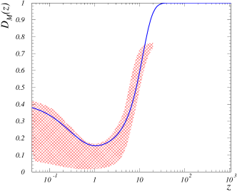
Figure 1: Depletion function $D_{M}$ vs redshift $z$. The line shows the $D_{M}(z)$ used in this work. It is constrained to remain within the $D_{M}(z)$ uncertainty determined in Ref. [11] (hatched band).

Accounting for the consequences of GR’s SI in the evolution of an inhomogeneous universe and of its large structures has been investigated using other methods than Eq. (3). Particularly, backreaction effects, which also originate from field SI, have been proposed to explain without dark energy the universe apparent acceleration, see review [19]. Most such studies are performed perturbatively and therefore omit the nonperturbative effects that are crucial in analogous QCD phenomena, e.g., quark confinement or the feebleness of hadron-hadron interaction comparatively to QCD’s strength. From this perspective, it is unsurprising that these studies do not find important effects from backreaction. While perturbative treatments of backreaction are already nontrivial, nonperturbative ones are more difficult but indicate that backreaction is important [20]. Although backreaction studies and our approach both investigate the consequence for dark energy of the $n>0$ terms of Eq. (2), the former approach assumes dark matter whereas the latter deduces, by solving nonperturbatively Eq. (2), that dark matter is also a consequence of GR’s SI [10]. The latter approach then identifies an explicit nonperturbative process (field trapping) that exposes a direct connection between dark matter and dark energy [11]. Aside investigations of backreation, other ideas have been proposed to explain the universe acceleration without dark energy, e.g., $f(R)$-gravity [21]. The key difference between these ideas and our approach is that they are beyond both GR, the current theory of gravity, and the Standard Model of Particle Physics (SMPP) since they postulate new fields to be yet detected. For example, while Eq. (2) is only a reexpression of GR’s Lagrangian, Eq. (1), [14], $f(R)$ theories add to Eq. (1) terms in powers of $R\equiv g_{\mu\nu}R^{\mu\nu}$ that go beyond GR, and requires “scalaron” fields and dark matter, both beyond the SMPP. This contrasts with our approach that is within both GR and the SMPP and connects dark energy and dark matter. Other extensions of GR than $f(R)$ theories may link dark energy to dark matter, e.g., [22] but so far they have not reproduced the CMB.

In the next section, we recall the expression of the CMB anisotropy correlation coefficient derived in the hydrodynamic approximation [23]. Then we discuss how SI modifies it and compare its computed values to the observations. In what follows, $t$ denotes time, $T$ the universe temperature, $a$ the Robertson-Walker scale factor, and $H$ the Hubble parameter, with $h$ its value in units of 100 km/s/Mpc. The subscripts $0$, $EQ$ and $L$ indicate values for the present, matter-radiation equilibrium, and last scattering times, respectively. $C^{s}_{TT,l}$ is the scalar multipole coefficient for the temperature-temperature angular correlation of the CMB anisotropies, with $l$ the multipole moment. The baryon, total matter, radiation, photon, cold dark matter, and dark energy densities relative to the critical density are $\Omega_{B}$, $\Omega_{M}$, $\Omega_{R}$, $\Omega_{\gamma}$, $\Omega_{DM}$, and $\Omega_{\Lambda}$, respectively, and $\Omega_{K}\equiv\nicefrac{{K}}{{a_{0}^{2}H_{0}^{2}}}$ with $K$ the metric curvature constant. Since dark matter and dark energy are not assumed, $\Omega_{DM}=0$ and $\Omega_{\Lambda}=0$ here.

III Effects of field self-interaction in the CMB anisotropies

An analytical expression of $C^{s}_{TT,l}$ is convenient since it allows us to see where and how the SI affects the CMB anisotropies. We use the approximate expression derived in Ref. [23]:

$$\frac{l(l+1)C^{s}_{TT,l}}{2\pi} = \frac{4\pi T_{0}^{2}N^{2}e^{-2\tau_{reion}}}{25}\int_{1}^{\infty}d\beta\bigg{(}\frac{\beta l}{l_{\mathcal{R}}}\bigg{)}^{n_{s}-1}\bigg{\{}\frac{3\sqrt{\beta^{2}-1}}{\beta^{4}(1+R_{L})^{\nicefrac{{3}}{{2}}}}\mathcal{S}^{2}(\beta l/l_{T})e^{-\nicefrac{{2\beta^{2}l^{2}}}{{l_{D}^{2}}}}\sin^{2}\big{(}\beta l/l_{H}+\Delta(\beta l/l_{T})\big{)}+$$ (4)

$$\frac{1}{\beta^{2}\sqrt{\beta^{2}-1}}\bigg{[}3\mathcal{T}(\beta l/l_{T})R_{L}-(1+R_{L})^{\nicefrac{{-1}}{{4}}}\mathcal{S}(\beta l/l_{T})e^{-\nicefrac{{\beta^{2}l^{2}}}{{l_{D}^{2}}}}\cos\big{(}\beta l/l_{H}+\Delta(\beta l/l_{T})\big{)}\bigg{]}^{2}\bigg{\}}+\mathcal{C}(l),$$

where $N$ is a factor normalizing the primordial perturbations, $\tau_{reion}$ is the optical depth of the reionized plasma, $l_{\mathcal{R}}=(1+z_{L})k_{\mathcal{R}}d_{A}$ with $k_{\mathcal{R}}\equiv 0.05$Mpc^-1 a conventional scale, and $d_{A}$ is the angular diameter distance of last scattering; $n_{s}$ is the scalar spectral index, $R_{L}=\nicefrac{{3\Omega_{B}}}{{4\Omega_{\gamma}(1+z_{L})}}$, $\mathcal{S},~{}\mathcal{T}$ and $\Delta$ are transfer functions, $l_{T}=\nicefrac{{d_{A}}}{{d_{T}}}$ with $d_{T}=\nicefrac{{\sqrt{\Omega_{R}}}}{{(1+z_{L})H_{0}\Omega_{M}}}$, $l_{D}=\nicefrac{{d_{A}}}{{d_{D}}}$ with $d_{D}$ the damping length, $l_{H}=\nicefrac{{d_{A}}}{{d_{H}}}$ with $d_{H}$ the acoustic horizon distance, and $\mathcal{C}(l)$ is a second-order correction not present in Ref. [23]. The first term in the curly bracket includes the Doppler effect, while the second term includes the Sachs-Wolf and intrinsic temperature anisotropy effects. Both terms include large-$l$ damping. Equation (4) is suited for the range $30\lesssim l\lesssim 2000$ since it does not include the integrated Sachs-Wolf, Sunyaev-Zel’dovich, and cosmic variance effects.

Although Eq. (4) without $\mathcal{C}(l)$ provides a good overall description of the CMB anisotropies [23], it is not fully accurate, hence the second-order correction $\mathcal{C}(l)$. It is numerically obtained by the difference between the first-order term in Eq. (4) and a formally exact numerical calculation of $\nicefrac{{l(l+1)C^{s}_{TT,l}}}{{2\pi}}$, e.g. [24], with both calculations performed with the $\Lambda$-CDM best fit parameters. It is sufficient for our purpose to restrict the SI corrections to the first-order term, since $\mathcal{C}(l)$ is by definition comparatively less dependent on cosmological parameters.

At the time of last scattering, GR’s SI effects are negligible. Thus, the mechanisms shaping Eq. (4) are unaffected and its form can be used as is. Since $\mathcal{S},~{}\mathcal{T}$, and $\Delta$ are time-independent and characterize the primordial scalar perturbations, the parameterizations [23] of these transfer functions also remain unmodified. On the other hand, the cosmological parameters and characteristic scales (distance or multipole) entering Eq. (4) are derived from present-day $z=0$ values and evolved back to $z=z_{L}$. It is through this evolution, which depends on the universe dynamics, that SI influences $C^{s}_{TT,l}$. The quantities affected are the angular diameter distance of last scattering $d_{A}$ (Eq. (5)), the damping length $d_{D}$, the scale $d_{T}$, the acoustic horizon distance (Eq. (6)), the $\Omega_{i}$, and the ratio $R_{L}$. Since $l_{\mathcal{R}}$, $l_{T}$, $l_{D}$ and $l_{H}$ involve $d_{A}$, $d_{T}$, $d_{D}$ or $d_{H}$, they are also affected by SI.

The distances $d_{A}$ and $d_{H}$ are given by:

$$d_{A}=\frac{1}{\sqrt{\Omega_{K}}H_{0}(1+z_{L})}\sinh\bigg{[}\sqrt{\Omega_{K}}\int^{1}_{1/(1+z_{L})}\frac{dx}{\sqrt{\Omega_{\Lambda}x^{4}+\Omega_{K}x^{2}+\Omega_{M}x}}\bigg{]},$$ (5)

$$d_{H}=\frac{2}{H_{0}(3R_{L}\Omega_{M})^{\nicefrac{{1}}{{2}}}(1+z_{L})^{\nicefrac{{3}}{{2}}}}\ln\big{(}[\sqrt{1+R_{L}}+\sqrt{R_{EQ}+R_{L}}]/[1+\sqrt{R_{EQ}}]\big{)}.$$ (6)

Two terms contribute to the damping length, $d_{D}\equiv\sqrt{d^{2}\textsubscript{Landau}+d^{2}\textsubscript{Silk}}$:

$$d^{2}\textsubscript{Landau}=\frac{3\sigma^{2}t_{L}^{2}}{8T_{L}^{2}(1+R_{L})},$$

where $\sigma$ is the standard deviation for the temperature $T_{L}$ owing to the fact that recombination was not instantaneous, and:

$$d^{2}\textsubscript{Silk}=\frac{R_{L}^{2}}{6(1-Y)(n_{B0})\sigma_{\mathcal{T}}H_{0}\sqrt{\Omega_{M}}R_{0}^{\nicefrac{{9}}{{2}}}}\int_{0}^{R_{L}}\frac{R^{2}dR}{X(R)(1+R)\sqrt{R_{EQ}+R}}\bigg{[}\frac{16}{15}+\frac{R^{2}}{1+R}\bigg{]},$$

where $Y\simeq 0.24$ is the density fraction for nucleons in neutral Helium, $n_{B0}$ the present baryon number density, $\sigma_{\mathcal{T}}$ the Thompson cross-section, $X$ the fractional ionization of the plasma, and $R(t)\equiv\nicefrac{{3\rho_{B}(t)}}{{4\rho_{\gamma}(t)}}$, with $\rho_{i}$ denoting average absolute densities. An approximation for $X$ is [25]:

$$X(T)\simeq\bigg{[}X(3400)^{-1}+\frac{\Omega_{B}}{\Omega_{M}^{1/2}}\int_{T}^{3400}\frac{84.2T^{\prime-0.1166}}{1+0.005085T^{\prime 0.53}+42200T^{\prime 0.8834}e^{-39474/T^{\prime}}}dT^{\prime}\bigg{]}^{-1}.$$ (7)

The SI affects $d\textsubscript{Silk}$ through $\Omega_{M}$, $R_{EQ}$, and $X$ since the latter depends on $\Omega_{M}$ and $\Omega_{B}$. The density ratio $R(t)$ is not affected by the SI because the SI leaves the evolutions of $\rho_{i}$ unaffected [11]. However, $R_{EQ}$ is affected since it is not defined as an absolute density ratio but as $R_{EQ}\equiv\Omega_{R}R_{0}/\Omega_{M}$. $R_{EQ}$ is identical to $R(t_{EQ})$ for a FLRW universe, but not anymore once SI is accounted for. In this case it must be redefined as:

$$R_{EQ}\equiv\frac{3\Omega_{R}\Omega_{B}}{4D_{M}(0)\Omega_{\gamma}(1+z_{L})}.$$

The distance $d\textsubscript{Landau}$ is affected by SI only [26] through the time of last rescattering,

$$t_{L}=\frac{1}{H_{0}}\int_{0}^{1/(1+z_{L})}x\big{[}\Omega_{\Lambda}x^{4}+\Omega_{K}x^{2}+\Omega_{M}x+\Omega_{R}\big{]}^{-\nicefrac{{1}}{{2}}}dx.$$

We now examine how SI specifically modifies the quantities just listed. SI is accounted for by replacing the $\Omega_{i}$ by the screened relative densities $\Omega^{*}_{M}(z)\equiv\Omega_{M}D_{M}(z)$, $\Omega^{*}_{B}(z)\equiv\Omega_{B}D_{M}(z)$ and $\Omega^{*}_{K}\equiv 1-\Omega_{R}-\Omega_{M}^{*}(z=0)$ [11]. $\Omega_{R}$ and $\Omega_{\gamma}$ remain unscreened because radiation does not aggregate. The $\Omega^{*}_{i}$ are effective dynamical quantities that enter in the evolution equation of the universe. Therefore, they should not be compared with densities obtained from censuses or primordial synthesis.

SI affects the parameters of Eq. (4) in two ways:
(1) it enhances local gravitational attraction;
(2) it globally suppresses gravity at large distances.
Effect (1) is important when the local universe density variation is large, i.e., for $t\gg t_{L}$. Since the mechanisms producing Eq. (4) occurred when density variation was small (the integrated Wolf-Sachs and Sunyaev-Zel’dovich effects are not included in Eq. (4)), effect (1) can be ignored. In other words, in the expressions formalizing the mechanisms generating the temperature anisotropies, $\Omega_{B}$ can remain since $\Omega^{*}_{B}(z\gg 1)\simeq\Omega_{B}$. Effect (2) influences the universe evolution and therefore affects how characteristic scales evolved since $t_{L}$. Thus, when $\Omega_{M}$ enters the expressions related to the evolution of the universe, it is replaced by $\Omega^{*}_{M}$. Since $\Omega_{M}$ is defined relative to the critical density for a FLRW universe, for a flat universe with $\Omega_{\Lambda}=0$ and $\Omega_{R}\ll 1$, $\Omega_{M}=1$ and $\Omega^{*}_{M}=D_{M}(z)$. (Note that for effect (2), $\Omega_{B}$ is irrelevant since it is not explicitly present in the universe evolution equation, being included in $\Omega_{M}$). Table 1 summarizes the expressions modified to account for SI.

Table 1: Expressions of the parameters explicitly affected by GR’s SI. Column 1: denominations. Column 2: standard expressions (FLRW universe). Column 3: expressions accounting for SI. For $X(T$), $g(T^{\prime})$ is the integrand in Eq. (7) and is unaffected by SI. The expressions for other parameters, such as characteristic multipoles or lengths, are not modified although their values change since their expressions involve quantities listed in the table.

	FLRW universe	Universe with GR’s SI accounted for
$d_{A}$	$\frac{1}{\sqrt{\Omega_{K}}H_{0}(1+z_{L})}\sinh\big{[}\sqrt{\Omega_{K}}\int^{1}_{1/(1+z_{L})}\frac{dx}{\sqrt{\Omega_{\Lambda}x^{4}+\Omega_{K}x^{2}+\Omega_{M}x}}\big{]}$	$\frac{1}{\sqrt{\Omega^{*}_{K}}H_{0}(1+z_{L})}\sinh\big{[}\sqrt{\Omega^{*}_{K}}\int^{1}_{1/(1+z_{L})}\frac{dx}{\sqrt{\Omega^{*}_{K}x^{2}+D_{M}(1/x-1)x}}\big{]}$
$d_{T}$	$\sqrt{\Omega_{R}}/[(1+z_{L})H_{0}\Omega_{M}]$	$\sqrt{\Omega_{R}}/[(1+z_{L})H_{0}D_{M}(0)]$
$d_{H}$	$\frac{2}{H_{0}(3R_{L}\Omega_{M})^{\nicefrac{{1}}{{2}}}(1+z_{L})^{\nicefrac{{3}}{{2}}}}\ln([\sqrt{1+R_{L}}+\sqrt{R_{EQ}+R_{L}}]/[1+\sqrt{R_{EQ}}])$	$\frac{2}{H_{0}(3R_{L}D_{M}(0))^{\nicefrac{{1}}{{2}}}(1+z_{L})^{\nicefrac{{3}}{{2}}}}\ln([\sqrt{1+R_{L}}+\sqrt{R_{EQ}+R_{L}}]/[1+\sqrt{R_{EQ}}])$
$R_{L}$	$[3\Omega_{B}]/[4\Omega_{\gamma}(1+z_{L})]$	$[3\Omega_{R}\Omega_{B}]/[4D_{M}(0)\Omega_{\gamma}(1+z_{L})]$
$t_{L}$	$\frac{1}{H_{0}}\int_{0}^{1/(1+z_{L})}x[\Omega_{\Lambda}x^{4}+\Omega_{K}x^{2}+\Omega_{M}x+\Omega_{R}]^{-\nicefrac{{1}}{{2}}}dx$	$\frac{1}{H_{0}}\int_{0}^{1/(1+z_{L})}x[\Omega^{*}_{K}x^{2}+D_{M}(1/x-1)+\Omega_{R}]^{-\nicefrac{{1}}{{2}}}dx$
$d^{2}\textsubscript{Silk}$	$\frac{R_{L}^{2}}{6(1-Y)(n_{B0})\sigma_{\mathcal{T}}H_{0}\sqrt{\Omega_{M}}R_{0}^{\nicefrac{{9}}{{2}}}}\int_{0}^{R_{L}}\frac{R^{2}dR}{X(R)(1+R)\sqrt{R_{EQ}+R}}\big{[}\frac{16}{15}+\frac{R^{2}}{1+R}\big{]}$	$\frac{R_{L}^{2}}{6(1-Y)(n_{B0})\sigma_{\mathcal{T}}H_{0}\sqrt{D_{M}(0)}R_{0}^{\nicefrac{{9}}{{2}}}}\int_{0}^{R_{L}}\frac{R^{2}dR}{X(R)(1+R)\sqrt{R_{EQ}+R}}\big{[}\frac{16}{15}+\frac{R^{2}}{1+R}\big{]}$
$X(T)$	$1/\big{[}X^{-1}(3400)+\frac{\Omega_{B}h^{2}}{(\Omega_{M}h^{2})^{1/2}}\int_{T}^{3400}g(T^{\prime})dT^{\prime}\big{]}$	$1/\big{[}X^{-1}(3400)+\frac{\Omega_{B}h^{2}}{(D_{M}(0)h^{2})^{1/2}}\int_{T}^{3400}g(T^{\prime})dT^{\prime}\big{]}$

We can now compute $C^{s}_{TT,l}$ with the SI effects included. The values of $T_{0}$, $\Omega_{\gamma}$ and $\Omega_{R}$ are well known from the measurement of the CMB average temperature. We use $T_{0}=2.7255$K [27], $\Omega_{\gamma}h^{2}=2.47\times 10^{-5}$ and $\Omega_{R}=1.6813\Omega_{\gamma}$ [23]. The remaining quantities ($H_{0}$, $n_{s}$, $z_{L}$ (or $T_{L}$), $\sigma_{t_{L}}$, $\Omega_{B}$ and $Ne^{-\tau_{reion}}$) are the free parameters to be determined by fitting the CMB data. The number of parameters is lower than for $\Lambda$-CDM since $\Omega_{DM}\equiv 0$, $\Omega_{\Lambda}\equiv 0$ and no assumption is needed for the thermodynamical properties of dark energy. In principle, $D_{M}(z)$, see Eq. (3), is fixed but in practice it can vary within its uncertainty, see Fig. 1. We used $z_{g}=8.5$, $\tau=4.5$, $A=0.25$ and $b=0.3$. Equation (4) with the expressions in the third column of Table 1 and $D_{M}(z)$ from Eq. (3) fits the scalar CMB anstropies for $\Omega_{B}=0.026$, $H_{0}=70$km/s/Mpc, $Ne^{-\tau_{reion}}=1.24\times 10^{-5}$, $n_{s}=0.97$, $z_{L}=1380$ and $\sigma/T_{L}=0.17$, see Fig. 2.

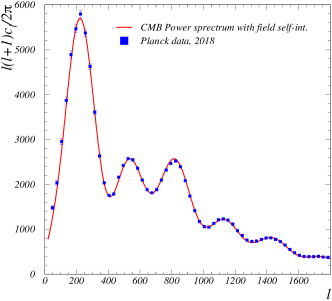
Figure 2: Power spectrum of the CMB temperature anisotropy. The red line is the present calculation, to be compared to the measurement (squares, Planck 2018 release [2]).

No uncertainties are assigned since our goal is not to provide a precise determination of cosmological parameters, but rather to determine if SI can be a natural and viable alternative to $\Lambda$-CDM.

IV Concordance with other observations

To be plausible, an alternative to $\Lambda$-CDM must account consistently for the observations related to dark matter and dark energy. Having examined the CMB anisotropies, the main object of this article, we now briefly discuss the consistency of the present approach with other important cosmological observations: the apparent magnitude of standard candles at large-$z$, large structure formation, the matter power spectrum $P(k)$, and the age of the universe. Except for $P(k)$, these observations were studied in detail in Refs. [11, 12] using the $D_{M}(z)$ originally determined in [11] (red hatched band in Fig. 1). Yet, although the band contains the $D_{M}(z)$ determined by our fit to the CMB observations (blue line in Fig. 1), the latter is more constrained and therefore need not provide results consistent with the other cosmological observations just mentionned. Nevertheless, the large-$z$ data [3, 28, 29] remain well described with the $D_{M}(z)$ determined by our CMB fit, see Fig. 3, left panel.

The effect of SI on structure formation was treated in Ref. [12]. The central panel of Fig. 3 shows the time-evolution of an overdensity of initial value $\delta(t_{L})=2\times 10^{-5}$ calculated with the $D_{M}(z)$ from our fit in Fig. 2 and without dark matter. This yields $\delta(t_{0})\approx 1$, consistent with the fact that structures had time to grow to their present densities.

The observation of the present distribution of structures, expressed by $P(k)$ where $k$ is the wavenumber, is another important constraint for cosmological models. As shown in the right panel of Fig. 3, the general shape of $P(k)$ can be described without dark matter/energy once SI effects are included. The reason is that the effects of Inflation on the early universe are unaffected by SI since the near uniformity and isotropy of the universe at early (post-inflation) times suppress SI effects (see Section II). Thus, at low $k$, $P(k)\propto k^{n_{s}}$ with $n_{s}=0.97$ from our CMB fit in Fig. 2. This is valid up to $k\lesssim k_{max}$ with, in the SI framework, $k_{max}=\sqrt{2}k_{EQ}=2H_{0}\sqrt{\Omega^{*}_{M}/a_{EQ}}$ [11] (where the effect of $n_{s}\neq 1$ can be neglected: $k_{max}$ increases by 1% for $n_{s}=0.97$), with $\Omega^{*}_{M}=D_{M}(0)$. Our CMB fit of Fig. 2 yields $k_{max}=0.014$hMpc^-1, in agreement with observations [30]. The spectrum maximum is given by $P(k_{max})=1.10\times 10^{14}[C(1/\Omega^{*}_{M}-1)N/h]^{2}/\Omega^{*}_{M}$ with $C(x)=\frac{5}{6}x^{-\nicefrac{{5}}{{6}}}\sqrt{1+x}\int_{0}^{x}\frac{du}{u^{\nicefrac{{1}}{{6}}}(1+u)^{\nicefrac{{3}}{{2}}}}$ [23]. With our CMB fit values, $P(k_{max})=2.4\times 10^{4}~{}(h^{-1}$Mpc$)^{3}$ [31]. The dissipative processes arising for $k>k_{max}$ involve in our case only non-relativistic baryonic matter, thus preserving the $P(k)\propto k^{-3}$ expected for $k>k_{max}$ from a nearly scale-invariant primordial power spectrum. While the detailed analysis of the finer structure of $P(k)$ is beyond the scope of this article, no difficulty is expected since that structure arises from baryon acoustic oscillations and Silk damping, both already well reproduced in Fig. 2.

Large-$z$ standard candles                 Large structure formation                     Matter power spectrum

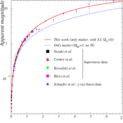
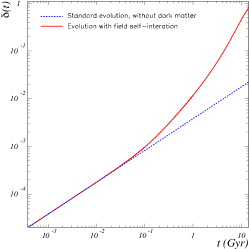
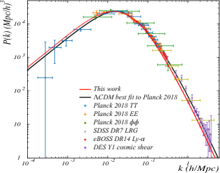
Figure 3: Left panel: Supernova apparent magnitudes vs. redshift. Also shown are $\gamma$-ray burst data (star symbols). The red line is the approach discussed here (universe containing only baryonic matter, with gravitational field self-interaction). The blue dotted line is for a flat FLRW universe with only matter. Central panel: Growth of an overdensity $\delta(t)$. Its initial value at the CMB emission time, $t_{L}\approx 3\times 10^{-4}$ Gyr, is $2\times 10^{-5}$. The red line shows the growth including self-interaction effects. The dotted line is without them. Right panel: Matter power spectrum vs. wavenumber. The data points are from the Planck [2], SSDS (LRG [32] and Li-$\alpha$ [33]), and DES [34] data compiled in [30]. The red line is the approach discussed here using the first order calculation [23]. The black line is the $\Lambda$-CDM best fit to the Planck data. The three red curves are not fitted to the data shown in the panels: the curves’ parameters are determined by the function $D_{M}(z)$ obtained from the CMB fit of Fig. 2.

Finally, the parameter values of our CMB fit in Fig. 2 yield an age of the universe after accounting for SI [11] of 12.8Gyr. This agrees with the oldest known objects whose ages are estimated independently of cosmological models, namely the chemical elements ($14.5^{+2.8}_{-2.5}$Gyr [35]), oldest stars ($13.5\pm 1$Gyr [36]), oldest star clusters ($12.8^{+0.9}_{-0.8}$Gyr [37]), and oldest white dwarfs ($12.8\pm 1.1$Gyr [38]).

V Conclusion

Our result shows that the CMB scalar anisotropies may be accurately explained without dark matter and dark energy once the field self-interaction of General Relativity is accounted for. The effect of the latter is folded in a universal function $D_{M}(z)$ that is obtained from the timescale of large structure formation and the relative amounts of baryonic matter present in these structures [11]. $D_{M}(z)$ is universal since it explains high-$z$ supernovae measurements [11] (Fig. 3, left panel), large structure formation [12] (Fig. 3, central panel), the shape of the matter power spectrum (Fig. 3, right panel), and the CMB anisotropies (Fig. 2). The SI of GR also eliminates the need for dark matter to explain the internal dynamics of structures: it straightforwardly yields flat rotation curves for disk galaxies [10], explains the empirical tight relation between baryonic and observed accelerations [9, 13], the Tully-Fisher relation [8, 10, 11], and accounts for the dynamics of galaxy clusters [10]. This framework is economical –no exotic matter, fields, nor modification of gravity are needed– and natural. Interestingly, QCD, whose Lagrangian’s structure is similar to that of GR, exhibits phenomena similar to those regarded as evidences for dark matter and dark energy.

Acknowledgments This work is funded in part by a Dominion Scholar grant from Old Dominion University. The author thanks C. Sargent, S. Širca and B. Terzić for useful discussions and for their comments on this article.

References

- [1] C. L. Bennett et al. “Four year COBE DMR cosmic microwave background observations: Maps and basic results,” Astrophys. J. Lett. 464, L1-L4 (1996); [astro-ph/9601067]; “Nine-Year Wilkinson Microwave Anisotropy Probe (WMAP) Observations: Final Maps and Results”. ApJ. 208 20 (2013) arXiv:1212.5225];
- [2] N. Aghanim et al., “Planck 2018 results. V. CMB power spectra and likelihoods,” Astron. Astrophys. 641, A5 (2020) [arXiv:1907.12875].
- [3] A. G. Riess, et al., “Observational evidence from supernovae for an accelerating universe and a cosmological constant”, AJ 116, 1009 (1998); [astro-ph/9805201]; S. Perlmutter, et al., “Measurements of and from 42 High-Redshift Supernovae,” ApJ 517 565 (1999) [astro-ph/9812133].
- [4] F. Kahlhoefer, “Review of LHC Dark Matter Searches,” Int. J. Mod. Phys. A 32, no.13, 1730006 (2017) [arXiv:1702.02430].
- [5] J. M. Gaskins, “A review of indirect searches for particle dark matter,” Contemp. Phys. 57, no.4, 496-525 (2016) [arXiv:1604.00014].
- [6] G. Arcadi et al. “The waning of the WIMP? A review of models, searches, and constraints,” Eur. Phys. J. C 78, no.3, 203 (2018) [arXiv:1703.07364].
- [7] A. A. Klypin, A. V. Kravtsov, O. Valenzuela and F. Prada, “Where are the missing Galactic satellites?,” Astrophys. J. 522, 82-92 (1999) [astro-ph/9901240].
- [8] R. B. Tully and J. R. Fisher, “A new method of determining distances to galaxies”, A&A, 54, 661 (1977)
- [9] S. McGaugh, F. Lelli and J. Schombert, “Radial Acceleration Relation in Rotationally Supported Galaxies,” Phys. Rev. Lett. 117, no. 20, 201101 (2016) [arXiv:1609.05917].
- [10] A. Deur, Implications of Graviton-Graviton Interaction to Dark Matter Phys. Lett. B 676, 21 (2009); [arXiv:0901.4005]; Self-interacting scalar fields at high-temperature Eur. Phys. J. C 77, 412 (2017); [arXiv:1611.05515]; “Relativistic corrections to the rotation curves of disk galaxies,” Eur. Phys. J. C 81, 213 (2021) [arXiv:2004.05905].
- [11] A. Deur, “An explanation for dark matter and dark energy consistent with the Standard Model of particle physics and General Relativity,” Eur. Phys. J. C 79, 883 (2019) [arXiv:1709.02481].
- [12] A. Deur, “Effect of gravitational field self-interaction on large structure formation,” Phys. Lett. B 820 (2021), 136510 [arXiv:2108.04649].
- [13] A. Deur, C. Sargent and B. Terzic, “Significance of Gravitational Nonlinearities on the Dynamics of Disk Galaxies,” Astrophys. J. , 896 2 94 (2020) [arXiv:1909.00095].
- [14] A. Zee, “Quantum Field Theory in a Nutshell”, 2003, Princeton University Press; A. Zee, “Einstein gravity in a Nutshell”, 2013, Princeton University Press
- [15] The universe evolution equation is based on GR and thus in principle includes the effect of SI. However, the usual FLRW model assumes complete isotropy and homogeneity. These approximations suppress the SI [10, 17, 13]. This is shown by the possibility to describe surprisingly well the universe evolution with the Newtonian theory, as first shown by E. A. Milne, “A NEWTONIAN EXPANDING universe” Q. J. Math 5, 1, 64 (1934)
- [16] P. J. Steinhardt, Critical Problems in Physics, V.L. Fitch. D. R. Marlow, and M. A.E. Dementi (eds.), 1997, Princeton University Press
- [17] A. Deur, “A relation between the dark mass of elliptical galaxies and their shape,” Mon. Not. Roy. Astron. Soc. 438, 2, 1535 (2014) [arXiv:1304.6932].
- [18] A. Dressler, et al., “Evolution since of the Morphology-Density relation for Clusters of Galaxies”, 1997, ApJ 490 577; [arXiv:astro-ph/9707232]; M. Postman, et al., The Morphology - Density Relation in 1 Clusters 2005, ApJ 623 721; [arXiv:astro-ph/0501224]; O. H. Parry, V. R. Eke, C. S. Frenk, “Galaxy morphology in the CDM cosmology”, MNRAS 396, 1972 (2009) [arXiv:0806.4189].
- [19] S. Schander and T. Thiemann, “Backreaction in Cosmology,” Front. Astron. Space Sci. 0, 113 (2021) [arXiv:2106.06043 [gr-qc]].
- [20] T. Buchert, et al. “Is there proof that backreaction of inhomogeneities is irrelevant in cosmology?,” Class. Quant. Grav. 32, 215021 (2015); [arXiv:1505.07800 [gr-qc]]. J. B. Mertens, J. T. Giblin and G. D. Starkman, “Integration of inhomogeneous cosmological spacetimes in the BSSN formalism,” Phys. Rev. D 93 no.12, 124059 (2016) [arXiv:1511.01106 [gr-qc]].
- [21] A. De Felice and S. Tsujikawa, “f(R) theories,” Living Rev. Rel. 13, 3 (2010) [arXiv:1002.4928 [gr-qc]].
- [22] E. P. Verlinde, “On the Origin of Gravity and the Laws of Newton,” JHEP 04, 029 (2011) [arXiv:1001.0785 [hep-th]].
- [23] S. Weinberg, “Cosmology,” Oxford Univ. Pr. (2008)
- [24] A. Lewis, A. Challinor and A. Lasenby, “Efficient computation of CMB anisotropies in closed FRW models,” Astrophys. J. 538, 473-476 (2000); [arXiv:astro-ph/9911177]; A. Lewis and S. Bridle, “Cosmological parameters from CMB and other data: A Monte Carlo approach,” Phys. Rev. D 66, 103511 (2002) [arXiv:astro-ph/0205436].
- [25] B. J. T. Jones and R. F. G. Wyse The ionisation of the primeval plasma at the time of recombination Astron. Astrophys. 149 144 (1985)
- [26] Although and are also affected by SI, the effect cancels in because it only involves the ratio .
- [27] P. A. Zyla et al. (Particle Data Group), Prog. Theor. Exp. Phys. 2020, 083C01 (2020)
- [28] M. Kowalski, et al., “Improved Cosmological Constraints from New, Old and Combined Supernova Datasets”, ApJ 686 749 (2008); [arXiv:0804.4142]; A. Conley, et al., “Supernova Constraints and Systematic Uncertainties from the First 3 Years of the Supernova Legacy Survey”, ApJS., 192, 1 (2011); [arXiv:1104.1443]; N. Suzuki, et al., “The Hubble Space Telescope Cluster Supernova Survey: V. Improving the Dark Energy Constraints Above and Building an Early-Type-Hosted Supernova Sample”, ApJ 746, 85 (2012) [arXiv:1105.3470].
- [29] B. E. Schaefer, “The Hubble Diagram to Redshift from 69 -Ray Bursts”, ApJ 660 16 (2007) [arXiv:astro-ph/0612285].
- [30] S. Chabanier, M. Millea and N. Palanque-Delabrouille, “Matter power spectrum: from Ly forest to CMB scales,” Mon. Not. Roy. Astron. Soc. 489, 2247 (2019) [arXiv:1905.08103]
- [31] For , where is an arbitrary reference wavenumber [23]. We use , as if . Also, as CMB scalar anisotropies cannot separate from and , we set to zero. (In -CDM, [2].)
- [32] B. A., Reid, et al., Cosmological Constraints from the Clustering of the Sloan Digital Sky Survey DR7 Luminous Red Galaxies Mon. Not. Roy. Astron. Soc. 404, 60 (2010) arXiv:0907.1659
- [33] S. Chabanier, et al., “The one-dimensional power spectrum from the SDSS DR14 Ly forests,” JCAP 07, 017 (2019) [arXiv:1812.03554].
- [34] M. A. Troxel et al. [DES], “Dark Energy Survey Year 1 results: Cosmological constraints from cosmic shear,” Phys. Rev. D 98 4, 043528 (2018) [arXiv:1708.01538].
- [35] N. Dauphas, The U/Th production ratio and the age of the Milky Way from meteorites and Galactic halo stars Nature 435, 1203 (2005)
- [36] M. Catelan, The ages of (the oldest) stars Proc. Int. Astr. Union, 13(S334), 11 (2017) [arXiv:1709.08656 ]
- [37] L. O. Kerber et al. A Deep View of a Fossil Relic in the Galactic Bulge: The Globular Cluster HP1 Mon. Not. Roy. Astron. Soc. 484 5530 (2019) [arXiv:1901.03721]
- [38] B. M. S. Hansen et al.,“HST observations of the white dwarf cooling sequence of M4,” Astrophys. J. Suppl. 155, 551 (2004) [arXiv:astro-ph/0401443]