Study of the ground state and thermodynamic properties of Cu5-NIPA-like molecular nanomagnets

Abstract

The thermodynamic properties of a spatially anisotropic spin-1/2 Heisenberg model for a Cu₅ pentameric molecule is studied through exact diagonalization. The elementary geometry of the finite lattice is defined on nanomolecules consisting of an hourglass structure of two corner-sharing scalene triangles which are related by inversion symmetry. This microscopic magnetic model is quite suitable to describe the molecular nanomagnetic compound Cu5-NIPA. The ground-state phase diagram, as well as the corresponding total magnetization, are obtained as a function of the anisotropic exchange interactions and the external magnetic field. The thermodynamic behavior of the model at finite temperatures is also studied and the corresponding magnetocaloric effects are analyzed for various values of the Hamiltonian parameters.

I Introduction

The experimental and theoretical studies of the intrinsic magnetism in large molecules and molecular nanomagnets have immensely increased in the last few decades [1, 2]. One of the main reasons for the great deal of appeal in these molecular nanomagnets resides in the possibility to experimentally access a wide variety of quite interesting fundamental quantum mechanical effects, such as quantum tunneling of the magnetization [3, 4, 5], quantum phase interference [6], level crossings and magnetization plateaux [7, 8], among others. What is even more appealing is the fact that these compounds turn out to be promising materials for several practical applications including, for instance, spintronics and quantum computing [1]. In addition, some of these molecular magnets exhibit also magnetocaloric effects [9, 10], which could make them highly suitable in designing a new era of magnetic refrigerators [10], operating not only at everyday room temperatures and temperatures of hydrogen and helium liquefaction (20 - 4.2 K), but also at subkelvin intervals needed in important low temperature experimental devices.

One of these highly interesting experimental realization of modern nanomagnetic materials is the chemical compound Cu₅(OH)₂(NIPA)${}_{4}\cdot$10H₂O, short named as Cu5-NIPA, with 5-NIPA standing for 5-nitro-isophtalic acid ligand. This system presents a rather uncommon pentameric form of a triangle-based structure, with a pair of corner-sharing scalene triangles, possessing an hourglass-like geometry. Some of the static magnetic properties of Cu5-NIPA molecules, including their spin dynamics behavior, have been investigated by Nath et al. [11]. Based on experimental results and ab initio density-functional band-structure calculations, a microscopic theoretical Heisenberg model, with spatially anisotropic exchange interactions, has been proposed to describe Cu5-NIPA. It has been shown that the Cu ions carry a spin-1/2 and, despite the triangular structure and ferromagnetic and antiferromagnetic interactions, the couplings lead to no magnetic frustation. This is in contrast, for example, to V6 like nanomolecules, where two independent triangles interact with exchange interactions causing molecular spin frustation [12, 13, 14, 15, 16].

More recently, Szałowski and Kowalewska [17] have studied the ground-state spectrum and the thermodynamic properties, including the magnetocaloric effects, of these molecular nanomagnets. They have considered, however, only the experimental exchange interaction values derived in Ref. [11] for the triangle bonds present in the Cu5-NIPA molecule. It would be thus quite interesting to see what will be the molecule behavior by considering different values for the coupling interactions, including sign change of the original ferromagnetic one, which will induce some magnetic frustration. As in ordinary magnetic materials, such variation of the exchange interactions could be physically plausible by controlling, for instance, some external conditions like the hydrostatic pressure. By using the exact diagonalization of the Hamiltonian, it will be shown that this molecule has indeed a very rich ground state phase diagram as a function of the model parameters, specially for the more symmetric case. Accordingly, the thermodynamics at finite temperatures also conveys interesting magnetocaloric effects, in its direct and inverse forms. We will here use a similar procedure recently employed in the study of V6 nanomolecules of Ref. [16].

The outline of this paper is as follows. In the next section, we describe the Hamiltonian model for the Cu5-NIPA-like molecules. In section III we present the exact analytical diagonalization for the energy spectrum and the corresponding more relevant eigenstates. The general behavior of the energy spectrum and the ground state phase diagram are discussed in section IV. In section V we investigate the magnetic and thermodynamic properties of the system through the study of the magnetization, susceptibility, entropy, magnetocaloric effect and specific heat. Finally, some concluding remarks are drawn in the last section.

II Hamiltonian model

The Cu5-NIPA-like magnetic molecules have five Cu²⁺ ions, carrying each one a spin-1/2, which are located at the vertices of two corner-sharing triangles, forming an hourglass structure, with inversion symmetry, as is schematically depicted in Fig. 1.

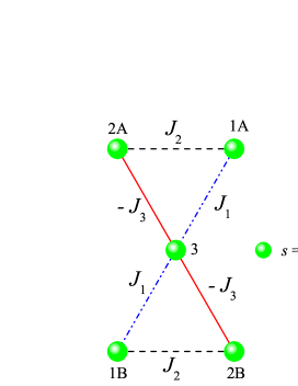
Figure 1: (color online) Schematic illustration of a Cu5-NIPA molecular magnet. The full circles represent the Cu²⁺ ions with spin-1/2. $A$ and $B$ denote the two triangles, with sites 1$A$, 2$A$, and 1$B$, 2$B$, respectively, both sharing the common site labeled as 3. $J_{1}$, $J_{2}$ and $J_{3}$ are the corresponding exchange interactions.

Based on the experimental results of Ref. [11], the corresponding Hamiltonian for this molecule can be written as

$$\mathcal{\hat{H}} = J_{1}(\vec{S}_{1A}\cdot\vec{S}_{3}+\vec{S}_{1B}\cdot\vec{S}_{3})+J_{2}(\vec{S}_{1A}\cdot\vec{S}_{2A}+\vec{S}_{1B}\cdot\vec{S}_{2B})$$

$$- J_{3}(\vec{S}_{2A}\cdot\vec{S}_{3}+\vec{S}_{2B}\cdot\vec{S}_{3})$$

$$- B(S_{1A}^{z}+S_{2A}^{z}+S_{1B}^{z}+S_{2B}^{z}+S_{3}^{z}),$$ (1)

where $J_{1}$, $J_{2}$ and $J_{3}$ are the exchange interactions and $B$ is the external magnetic field applied in the $z$ direction. $\vec{S}=(S_{i}^{x},S_{i}^{y},S_{i}^{z})$ is the Heisenberg spin-1/2 operator with the components $S_{i}^{\alpha}$ ($\alpha=x,y,z$) given by the Pauli spin matrices.

Specifically for the Cu5-NIPA molecule all the exchange interaction parameters in Hamiltonian (1) are positive and are given by $J_{1}=217$ K and $J_{2}=J_{3}=62$ K, which results in a non-frustrated molecule, despite the triangle structure with some antiferromagnetic interactions. In this work, we will study the effects of different exchange interactions in this kind of molecule, allowing still for the presence of frustration with negative values of $J_{2}$ and $J_{3}$, and analyzing the corresponding effects in the zero temperature phase diagram as well as in the thermodynamic behavior of the system.

III Eigenenergies and eigenstates

Using the eigenstates of the $z$-component $S^{z}_{i}$ spin operator that spam the Hilbert space of $\cal H$, the above Hamiltonian is given by a $32\times 32$ matrix that can be exactly diagonalized by resorting to some modern technical computing system like Maplesoft. This procedure has been previously done in Refs. [11, 17]. However, as in the present study we will consider general values for the exchange interactions and external magnetic field, the 32 eigenvalues so obtained are explicitly given in the Appendix.

Concerning the eigenstates, even if we omit those coming from the cumbersome solution of the cubic equation (21), the remainder ones are still rather lengthy to be reproduced in the Appendix. For this reason, we will present below only the corresponding eigenstates of the more relevant low-lying eigenenergies, and grouping them according to their total spin values $S$, since it is the quantity $S$ that gives the main magnetic behavior of the molecule.

III.0.1 Ferromagnetic state with $S=5/2$

There is one state with all spins aligned with the magnetic field resulting in a molecular total spin $S=5/2$. This ferromagnetic (FM) state has energy $E_{FM}$ and eigenstate $\ket{FM}$, which are respectively given by

$$E_{FM}=\varepsilon_{1}=\frac{1}{2}J_{1}+\frac{1}{2}J_{2}-\frac{1}{2}J_{3}-\frac{5}{2}B,$$ (2)

$$|FM\rangle=|\uparrow,\uparrow,\uparrow,\uparrow,\uparrow\rangle,$$ (3)

where an up arrow represents the $z$-component of the spin aligned in the same direction of the external magnetic field (a down arrow means the opposite). This will be the stable phase for large magnetic fields.

III.0.2 Ferrimagnetic state with $S=3/2$

This ferrimagnetic (FI1) state has spin-3/2 with eigenenergy $E_{FI1}$ and eigenstate $\ket{FI1}$ given by

$$E_{FI1}=\varepsilon_{11}=-\frac{1}{4}J_{1}+\frac{1}{4}J_{3}-\frac{3}{2}B-\frac{1}{4}r,$$ (4)

$$|FI1\rangle= \dfrac{1}{\sqrt{2a^{2}+b^{2}+2}}[|\uparrow,\uparrow,\uparrow,\downarrow,\uparrow\rangle$$

$$+|\downarrow,\uparrow,\uparrow,\uparrow,\uparrow\rangle-a|\uparrow,\uparrow,\uparrow,\uparrow,\downarrow\rangle$$

$$-a|\uparrow,\downarrow,\uparrow,\uparrow,\uparrow\rangle+b|\uparrow,\uparrow,\downarrow,\uparrow,\uparrow\rangle],$$ (5)

where

$$a= \dfrac{3J_{1}+3J_{3}+r}{2(J_{2}+2J_{3})}$$ (6)

$$b= \dfrac{3J_{1}-2J_{2}-J_{3}+r}{J_{2}+2J_{3}}$$ (7)

$$r= \sqrt{(J_{1}+J_{3})^{2}+4J_{2}^{2}+8[J_{1}^{2}+J_{3}^{2}-J_{2}(J_{1}-J_{3})]}.$$ (8)

III.0.3 Ferrimagnetic state with $S=1/2$

There is another ferrimagnetic state (FI2) with smaller total spin value given by

$$E_{FI2}= \varepsilon_{31}=x_{3}-\frac{1}{2}B,$$ (9)

$$|FI2\rangle= \leavevmode\nobreak\ c_{1}|\uparrow,\downarrow,\uparrow,\uparrow,\downarrow\rangle+c_{2}|\uparrow,\downarrow,\uparrow,\downarrow,\uparrow\rangle$$

$$+ \leavevmode\nobreak\ c_{3}|\downarrow,\uparrow,\uparrow,\downarrow,\uparrow\rangle+c_{4}|\downarrow,\uparrow,\downarrow,\uparrow,\uparrow\rangle,$$ (10)

where $x_{3}$ is the smallest solution of the cubic equation (21) and $c_{i}$, $i=1,2,3,4$, are constants satisfying the normalization condition $\sum_{i=1}^{4}c_{i}^{2}=1$. Due to the awkward solutions of the cubic equation, this state, as well as the degenerated one described below, have been numerically computed for general values of the exchange interactions.

III.0.4 Degenerate ferrimagnetic state with $S=1/2$

This phase (FID) occurs in the ground state only for $J_{3}=-J_{1}$, where one has

$$E_{FID}=\varepsilon_{21}=\varepsilon_{27}=-J_{1}-\frac{1}{2}J_{2}-\frac{1}{2}B,$$ (11)

with two different eigenstates

$$|FID_{1}\rangle=\dfrac{1}{\sqrt{6}}[ - |\uparrow,\uparrow,\downarrow,\uparrow,\downarrow\rangle+|\uparrow,\uparrow,\downarrow,\downarrow,\uparrow\rangle$$ (12)

$$- \left.|\uparrow,\downarrow,\uparrow,\uparrow,\downarrow\rangle+|\uparrow,\downarrow,\downarrow,\uparrow,\uparrow\rangle\right.$$

$$- |\downarrow,\uparrow,\uparrow,\uparrow,\downarrow\rangle+|\downarrow,\uparrow,\uparrow,\downarrow,\uparrow\rangle],$$

and

$$|FID_{2}\rangle=\dfrac{1}{\sqrt{6}}[ + |\uparrow,\uparrow,\downarrow,\uparrow,\downarrow\rangle-|\uparrow,\uparrow,\downarrow,\downarrow,\uparrow\rangle$$ (13)

$$- |\uparrow,\downarrow,\uparrow,\downarrow,\uparrow\rangle+|\uparrow,\downarrow,\downarrow,\uparrow,\uparrow\rangle$$

$$- |\downarrow,\uparrow,\uparrow,\uparrow,\downarrow\rangle+|\downarrow,\uparrow,\downarrow,\uparrow,\uparrow\rangle],$$

where, in this case, the smallest eigenvalue of the cubic equation has been labeled as $x_{1}$. Note that for $J_{3}=-J_{1}$ the molecule is more symmetric resulting in a much simpler analytical expression for the eigenvalues and eigenstates.

IV Energy spectrum and ground state phase diagram

In what follows, we will fix our energy scale by assigning the value $J_{1}=1$ or, in other words, measuring the other exchange interactions, including the magnetic field, in units of $J_{1}$.

IV.1 Energy spectrum

Fig. 2 shows the complete set of energy levels, which is formally given in the Appendix, as a function of the external magnetic field $B$, for different values of the exchange interactions $J_{2}$ and $J_{3}$. The most relevant low-lying states for our purpose are highlighted according to the legend on top of panels (a) and (b). One can see that, for large values of the external magnetic field, the stable phase is the ferromagnetic one, regardless the strength of the exchange interactions. For $J_{2}=J_{3}=1$ in Fig. 2(a), as the external field increases from zero, the molecule undergo a first-order phase transition from the state FI2 to FI1, following another phase transition from FI2 to FM. Note that as $B$ increases, so does the total molecular spin $S$, the latter one jumping from 1/2 to 3/2 in the first transition, and from 3/2 to 5/2 in the second transition, as should be expected.

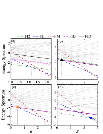
Figure 2: (color online) Energy spectrum as a function of the external magnetic field $B$, for some values of the exchange interactions $J_{2}$ and $J_{3}$. We have in (a) $J_{2}=1$ and $J_{3}=1$; in (b) $J_{2}=0.8$ and $J_{3}=-1$; in (c) $J_{2}=1$ and $J_{3}=-1$ and in (d) $J_{2}=2$ and $J_{3}=-1$. The legend of the low-lying states are given on top of panels (a) and (b). The energy of both FID phases are the same in (b)-(c), and are also equal to the energy of FI2 phase for $J_{2}=1$ in (c). The triangle in (b), the square in (c) and the star in (d) represent triple, quadruple and quintuple points, respectively. All other crossings are ordinary two-phase coexistence.

It is interesting to see what happens when $J_{3}=-1$, making the molecule more symmetric but inducing, at the same time, a frustration in the ordering of the $z$-component spin of Cu ions. This is shown in Figs. 2(b), (c) and (d) for increasing values of $J_{2}$, namely $J_{2}=0.8,\leavevmode\nobreak\ 1$, and 2. For $J_{3}=-1$, the two FID phases have the same energies and are the ground state for small fields for $J_{2}=0.8$. The triangle in Fig. 2(b) signals the triple point where the molecule transitions to the FI2 phase. However, for $J_{2}=1$ the FID phases also coexist with the FI2 phase in a triple line for low magnetic fields, before transitioning to the FI1 phase at the quadruple point represented by the square in 2(c). For $J_{2}=2$, the FID and FI1 phases are suppressed as the lowest energies, and only a transition from FI2 to the FM phase takes place. However, at this transition, the energy of FI1 phase, as well as the eigenenergies $\epsilon_{7}$ and $\epsilon_{9}$ (which are not highlighted in the other panels because they are only significant for this case), are all the same, turning this transition into a quintuple point, which is given by the star in 2(d).

IV.2 Ground state phase diagram

From Fig. 2 it is easy to see that we can construct the phase diagram, in terms of the Hamiltonian parameters, by just seeking the crossing values of the energies of the states FM, FI1, FI2 and FID. This is easily achieved by equating the corresponding low-lying eigenenergies. As a matter of example, the transition from FI1 to the FM phase is given by

$$B=\dfrac{3}{4}J_{1}+\dfrac{1}{2}J_{2}+\dfrac{3}{4}J_{3}+\dfrac{1}{4}r.$$ (14)

The other transition lines involve the numerical solutions of Eq. (21).

Fig. 3 depicts the topology of the phase diagram in the $J_{2}$ versus $B$ plane for different values of the interaction $J_{3}$. For positive values of $J_{3}$, the phase diagrams are quite similar to that shown in Fig. 3(a) for $J_{3}=1$. The FI1 phase lies always between the FI2 and FM phases and their boundaries correspond to two-phase coexistence lines. High positive values of $J_{2}$ force the $z$-component of the spins in sites $1A$ and $2A$ to be antiferromagnetically ordered, with the same ordering for the sites $1B$ and $2B$. For positive values of $B$ the total spin of the molecule will then be $S=1/2$, the FI2 phase. On the other hand, for negative values of $J_{2}$, a ferromagnetic ordering will prevail between sites $1A$ and $2A$, as well as between sites $1B$ and $2B$, implying that for small values of $B$ the FI1 phase with $S=3/2$ will be stable instead. As expected, for strong external magnetic fields the tendency is the molecule to be in the FM phase.

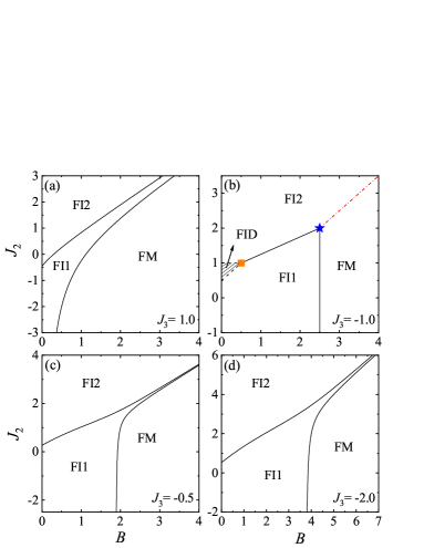
Figure 3: (color online) Ground-state phase diagram in the $J_{2}$ versus $B$ plane. The full lines represent transitions where two phases coexist, the dashed lines where three phases coexist (triple line), and the dashed-dotted line has four phases coexisting (quadruple line). Accordingly, the square is a quadruple point and the star is a quintuple point. The hatched area is a region where the two FID phases coexist. The values of $J_{3}$ are given in the bottom right of each panel.

The interesting case $J_{3}=-1$ is depicted in Fig. 3(b), where one has a region of the two FID phases coexisting for low magnetic fields. These two-coexisting phases are separated from the single FI2 and FI1 phases by triple lines. These triple lines meet the two-phase transition line from the FI2 to FI1 phases in a quadruple point. The transition line from the FM phase to the FI2 phase is in fact a quadruple line, because in addition to the coexistence of the FM and FI2 phase, we still have the eigenenergies $\epsilon_{7}$ and $\epsilon_{9}$ being equal to the energies FI2 and FM in this parameter region. As a result, the common point of the FI1, FI2 and FM phases in Fig. 3(b) turns out to be a quintuple point. A more detailed view of the coexisting phases at the above quadruple and quintuple points can be seen in Figs. 2(c) and (d), respectively.

For $J_{3}\neq-1$ the phase diagrams are similar to that shown in Fig. 3(a), as can be seen in Figs. 3(c) and (d) for $J_{3}=-0.5$ and $J_{3}=-2$, respectively. The main difference is the narrowing of the FI1 phase region, between the FI2 and FM phases, for large values of the external magnetic field.

V Thermodynamic properties

The thermodynamic properties of these magnetic molecules can be obtained by calculating the partition function through

$$\mathcal{Z}=\sum_{i=1}^{32}\mathrm{e}^{-\beta\varepsilon_{i}},$$ (15)

where $\beta=1/k_{B}T$, $k_{B}$ is the Boltzmann constant, $T$ is the absolute temperature, and $\varepsilon_{i}$ are all the eigenvalues of the present Hamiltonian (which are given in the Appendix). Although in the literature Eq. (15) is referred to as the canonical ensemble partition function, the proper designation for this ensemble would be field ensemble, as discussed in Ref. [18]. However, independent of the given ensemble name, the corresponding free energy per molecule will be given by

$$F=F(T,B)=-k_{B}T\ln(\mathcal{Z}).$$ (16)

From the above free energy, we can compute all thermodynamic quantities of interest. In the present case we will analyse the magnetization $M$ and susceptibility $\chi$, entropy $\mathcal{S}$ and specific heat $C$, which can be calculated from the well known thermodynamic relations

$$M = -\left(\dfrac{\partial F}{\partial B}\right)_{T},\quad\chi=\left(\dfrac{\partial M}{\partial B}\right)_{T},\quad$$ (17)

$$\mathcal{S} = -\left(\dfrac{\partial F}{\partial T}\right)_{B},\quad C=T\left(\dfrac{\partial S}{\partial T}\right)_{B}.$$ (18)

An interesting quantity that can be studied in this system is the so called magnetocaloric effect, which is defined by the adiabatic temperature change, or the isothermal entropy change, as the external magnetic field is varied. This effect can be quantified by the following relation

$$\left(\frac{\partial T}{\partial B}\right)_{S}=-\frac{(\partial S/\partial B)_{T}}{(\partial S/\partial T)_{B}}.$$ (19)

Another quantity related to the magnetocaloric effect is the change of the magnetic entropy due to a change in the magnetic field and can be written as

$$\Delta S(T,\Delta B) = \int_{B_{i}}^{B_{f}}\left(\dfrac{\partial M(T,B)}{\partial T}\right)_{B}dB$$ (20)

$$= S(T,B_{f})-S(T,B_{i}),$$

where $\Delta B=B_{f}-B_{i}$, $B_{i}$ and $B_{f}$ being the initial and final magnetic fields, respectively [19, 20]. When $-\Delta S>0$ the material has a conventional, or direct, magenetocaloric effect (the system heats up), and when $-\Delta S<0$ the material presents an inverse magnetocaloric effect (the system cools down).

In what follows we will present the thermodynamic behavior of the model described by the Hamiltonian (1). In all the results discussed below we considered $k_{B}=1$ in order to have $k_{B}T/J_{1}\rightarrow T$. We have also taken the more interesting case $J_{3}=-1$, however, the general trend of the results are qualitatively similar for other values of $J_{3}$.

V.1 Magnetization

Looking at the ground state phase diagrams depicted in Fig. 3, one can see that, in general, for small values of $J_{2}$, mainly negative ones, one has only one first-order transition from the $S=3/2$ to the $S=5/2$ state, while for higher values of $J_{2}$ one has two transitions, since $S=1/2$ is also a stable phase for small values of $B$. Exception should be made for $J_{3}=-1$ and $J_{2}>2$, where only one transition is seen from the $S=1/2$ to the $S=5/2$ state. However, as discussed in the previous section, at this latter transition there is also a coexistence with phases given by the eigenenergies $\epsilon_{7}$ and $\epsilon_{9}$, where both correspond to eigenstates with $S=3/2$. Overall, at zero temperature, the magnetization, as a function of $B$, has a stepwise shape with either two or three steps.

In Fig. 4 we have the magnetization, as a function of external field, for $J_{3}=-1$ and different values of the exchange interaction $J_{2}$ and temperature T. In the ground state we have $M=S$ and the magnetization has a stair style clearly showing the jumps of $M$ at the transitions. However, as soon as we have a finite temperature, a continuous behavior takes place. At the same time, the magnetization drops to zero at $B=0$ for any value of $T$. This is indeed an expected behavior, because being the molecule a zeroth dimensional quantum system, it is equivalent to a one-dimensional classical spin model, which in turn has no phase transition at finite temperatures. However, it is worthwhile to see that for low temperatures, the system still keeps a kind of memory of the ground state magnetization. The experimental results of the measured magnetization of the Cu5-NIPA compound in Ref. [11] show exactly the above behavior as the magnetic field increases from zero. Although only the transition from the FI2 to the FI1 has been observed, the next transition to the FM phase should probably occur for still higher values of the magnetic field.

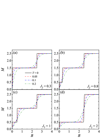
Figure 4: (color online) Total molecular magnetization $M$, as a function of the magnetic field $B$, for $J_{3}=-1$ and different values of temperature $T$ and exchange interaction $J_{2}$. The legend of the temperatures shown in (a) also applies to the other panels.

It is interesting to notice that the behavior of the magnetization, now as a function of the temperature, has some peculiarities for external fields just smaller than the fields where the jump occurs. For these values of $B$, the magnetization, as a function of temperature, initially increases before smoothly start to decrease to zero. This is shown in Fig. 5 for several values of the external field (this figure takes the same exchange parameters as Fig. 4). This unusual increase of $M$ with $T$ reflects the fact that, in this region, the thermal fluctuations initially populate states having higher values of $S$.

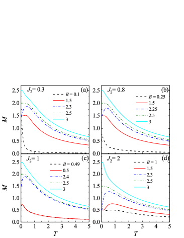
Figure 5: (color online) Total molecular magnetization $M$, as a function of temperature $T$, for $J_{3}=-1$ and different values of the external fields and exchange interaction $J_{2}$.

For $J_{3}\neq-1$ the behavior of the magnetization is quite similar to those shown in Figs. 4 and 5.

V.2 Susceptibility

The susceptibility times temperature, as a function of the temperature (in logarithmic scale for a better visualization of the whole range of $T$), is shown in Fig. 6 for $J_{3}=-1$ and various values of external field and exchange interaction $J_{2}$. For high values of temperature one has the usual paramagnetic behavior for any values of the external field, as expected. For low temperatures, one has $\chi T\rightarrow 0$ as $T\rightarrow 0$ for all values of $B$, except those where the molecule magnetization changes its total spin value at zero temperature. At these transition fields we can clearly see that $\chi T\rightarrow constant$. Note, however, that this is not a quantum critical phase transition, being only an ordinary first-order transition (recall that for the one-dimensional Ising model one has $\chi T\rightarrow\infty$ as $T\rightarrow 0$ [21]).

As $T\rightarrow 0$ the susceptibility can be analytically obtained through an expansion of the partition function at low temperatures. It turns out that, in this limit, $\chi$ is independent of the exchange interactions $J_{2}$ and $J_{3}$, depending only on the constant prefactor multiplying the magnetic field. Since $\chi T\rightarrow 1.25$ as $T\rightarrow 0$ for $B=0$ and $J_{2}=0.3$ in Fig. 6(a), and this value of the susceptibility is comparable to the value at high temperatures, one can see a valley like behavior for intermediate values of $T$. On the other hand, for $B=0.1$ the susceptibility should go to zero as $T\rightarrow 0$, in some sense explaining the peak and valley present in Fig. 6(a). In the other panels of Fig. 6, the plateau at $T=0$ is responsible for the presence of the shoulder for external fields close to the quantum phase transition ones.

It should be said that the experimental results of $\chi T$ obtained from Cu5-NIPA samples [11] display indeed the general form shown in Fig. 6, but without the presence of any valley or shoulder.

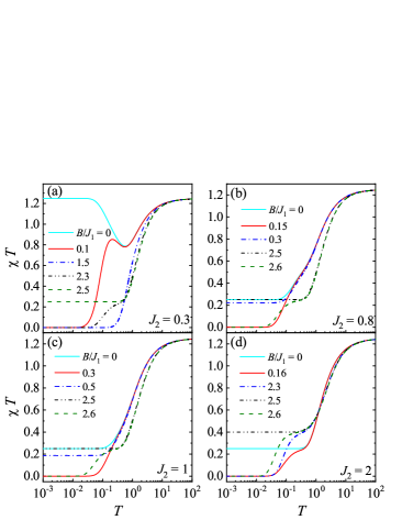
Figure 6: (color online) Susceptibility times temperature $\chi T$, as a function of temperature $T$ (in logarithmic scale), for $J_{3}=-1$ and different values of the magnetic field $B$ and exchange interaction $J_{2}$.

V.3 Entropy

The entropy, as a function of temperature, is shown in Fig. 7 for different values of external field and exchange interaction $J_{2}$. In all cases, for high temperatures, the entropy approaches the expected value $\mathcal{S}=\ln\omega$ with $\omega=32$, since in this limit all states are equally probable. On the other hand, as $T$ goes to zero, one can see a residual entropy occurring at the transition lines and regions of phase coexistence, compatible with the results shown in Fig. 3(b), with now $\omega$ being the degeneracy of the ground state

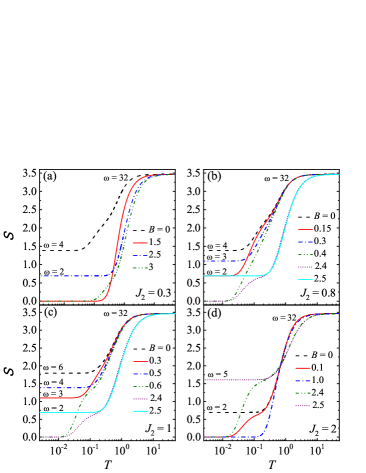
Figure 7: (color online) Entropy $\mathcal{S}$ as a function of temperature $T$ (in logarithmic scale) for $J_{3}=-1$ and different values of the magnetic field $B$ and exchange interaction $J_{2}$. $\omega$ gives the degeneracy of the ground state (and also the number of states at high temperatures).

In Fig. 8 we have the entropy, in a gradient scale, for two different low temperatures and the parameters of Fig. 3(b), keeping in the background the zero temperature phase diagram. We can see that the entropy at low temperatures is indeed higher near the lines of the phase transitions in the region FID where several phases coexist.

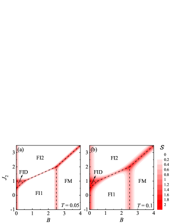
Figure 8: (color online) Density plot of the entropy $\mathcal{S}$, in a color gradient scale shown to the right, for two low temperatures, keeping in the background the phase diagram of Fig. 3(b), using here only dashed lines for the transition boundaries.

Looking back to Fig. 7, we can see that in (a)-(c) the entropy for $B=0$ is above the entropy for greater values of $B$, implying that in this case one has a conventional magnetocaloric effect. On the other hand, in (d) the entropy for $B=0$ is, in some intervals of $T$, below the corresponding entropy of some greater external fields. As a consequence, in these regions we have the inverse magnetocaloric effect.

A more detailed view of the entropic behavior can be seen in Fig. 9. In this figure, we have in fact the density plot of entropy, in a color gradient scale, as a function of $B$ and $T$ for $J_{3}=-1$. Some constant entropy lines are also highlighted in that figure and all lines meet, for low temperatures, at the transition magnetic field values given in Fig. 3(b).

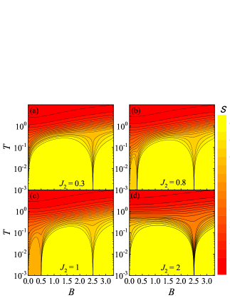
Figure 9: (color online) Density plot of the entropy, in a color gradient scale shown to the right, as a function the magnetic field $B$ and the temperature $T$ (in logarithmic scale) for $J_{3}=-1.0$ and different values of the exchange interaction $J_{2}$. Some lines of constant entropy are also plotted.

V.4 Magnetocaloric effect

Although some aspects of the magnetocaloric effect could already be seen from the analysis of Fig. 7, more information can be obtained by computing the variation of the magnetic entropy with the external field defined in Eq. (20). The change in the magnetic entropy $-\Delta{\mathcal{S}}$ as a function of temperature for different values of the final magnetic field is shown in Fig. 10. In all cases we have considered zero initial magnetic field. As discussed in the previous subsection, in Figs. 10(a)-(c) only direct magnetic caloric effect is present, because of the positiveness of $-\Delta\mathcal{S}$. However, in (d) we clearly have an inverse magnetocaloric effect for some regions of temperature, since in this case $-\Delta\mathcal{S}<0$. As for high temperatures the entropy is the same, regardless the value of the external field, one has in this limit $-\Delta\mathcal{S}=0$ for any value of $B$. On the other hand, in the limit of zero temperature $-\Delta\mathcal{S}$ is different from zero, due to the ground state degeneracy at $B=0$.

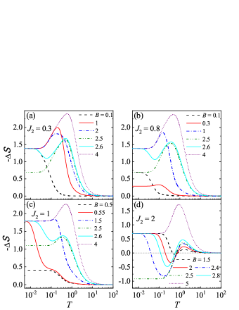
Figure 10: (color online) Isothermal change of the entropy $-\Delta\mathcal{S}$, as a function of the temperature $T$ (in logarithmic scale), for several values of the final magnetic field $B$ and considering a zero value for the initial magnetic field.

We can see from Fig. 10 that for small final fields the change in the magnetic entropy presents a peak; for intermediate fields, generally about the phase transition region, a minimum develops before the peak; and for still higher values of fields only one peak is again observed. This is better seen in Fig. 11, where we have the density plot of the change in the magnetic entropy $-\Delta\mathcal{S}$ as a function of the final magnetic field $B$ and the temperature $T$ (in logarithmic scale) for $J_{3}=-1.0$ and $J_{2}=2$. The inset in this figure shows the specific case of the entropies and the magnetic entropy change for $B=2.4$ (close to the transition field $B=2.5$) as a function of temperature. The minimum happens because the entropy for the field in this region starts to increase before the zero field entropy and, in some cases, they even cross, as shown in this inset. In the more detailed view of Fig. 11, the region inside the dashed line corresponds to inverse magnetocaloric effect. For different values of the exchange parameters than those of Fig. 7, we only observe the direct magnetocaloric effect.

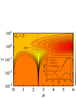
Figure 11: (color online) Density plot of the change in magnetic entropy $\Delta\mathcal{S}$, in a color gradient scale shown to the right, as a function the final magnetic field $B$ and the temperature $T$ (in logarithmic scale) for $J_{3}=-1.0$ and $J_{2}=2$. Some lines of constant magnetic entropy change are also plotted. The dashed line corresponds to zero entropy variation. redThe inset shows the entropies and the magnetic entropy change for $B=2.4$ (close to the transition field $B=2.5$) as a function of temperature.

V.5 Specific heat

Having computed the entropy as a function of temperature it is interesting to see the behavior of the specific heat for these molecules. Fig. 12 shows $C$ as a function of temperature for $J_{3}=-1$ and various values of external field and exchange interaction $J_{2}$. In all cases the specific heat goes to zero in the limits of high and low temperatures, as should be the case for any system having a finite energy spectrum. A Schottky behavior with only one maximum is noted for those values of external fields where the entropy has no shoulder as function of temperature. The double peak topology, for certain values of $B$, reflects exactly the shoulder present in the curves depicted in Fig. 7. The double peak topology for certain values of $B$ reflects the shoulders present in the curves depicted in Fig. 7. The experimental results of the specific heat for the Cu-5NIPA compounds of Ref. [11] only show the low temperature behavior of $C$. Experimental results for higher values of $T$ should evidence a kind of Schottky peak for the fitted exchange interactions.

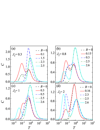
Figure 12: (color online) Specific heat $C$ as a function of temperature $T$ (in logarithmic scale) for various values of the magnetic field $B$ for $J_{3}=-1.0$.

VI Concluding remarks

A quantum spatially anisotropic spin-1/2 Heisenberg model, suitable for describing Cu₅ pentameric molecules, in the presence of an external magnetic field applied along the $z$-axis, has been studied through exact diagonalization of the Hamiltonian. A wider range for the exchange interactions has been considered. The behavior of the system at zero temperature has been determined through its energy spectrum and a detailed analysis of the corresponding phase diagrams for different coupling values. The model presents not only a rich phase diagram, but also residual entropies at zero temperature. The thermodynamic properties at finite temperatures have also been obtained by computing the magnetization, susceptibility, entropy, magnetocaloric effect and specific heat. Depending on the values of the exchange interactions these molecules can exhibit either direct or inverse magnetocaloric effect. It is expected that the Hamiltonian (1), despite being a quite simple example of a zero-dimensional quantum system, could also be applied to low dimensional quantum models such as triangular chains.

*

Appendix A

The eigenvalues $\epsilon_{i}$ of the Hamiltonian (1), with $1\leq i\leq 32$, can be written as

$$\varepsilon_{1}= \frac{1}{2}J_{1}+\frac{1}{2}J_{2}-\frac{1}{2}J_{3}-\frac{5}{2}B$$

$$\varepsilon_{2}= \frac{1}{2}J_{1}+\frac{1}{2}J_{2}-\frac{1}{2}J_{3}+\frac{5}{2}B$$

$$\varepsilon_{3}= \frac{1}{2}J_{1}+\frac{1}{2}J_{2}-\frac{1}{2}J_{3}-\frac{3}{2}B$$

$$\varepsilon_{4}= \frac{1}{2}J_{1}+\frac{1}{2}J_{2}-\frac{1}{2}J_{3}+\frac{3}{2}B$$

$$\varepsilon_{5}= \frac{1}{4}J_{1}-\frac{1}{4}J_{3}-\frac{3}{2}B+\frac{1}{4}p$$

$$\varepsilon_{6}= \frac{1}{4}J_{1}-\frac{1}{4}J_{3}+\frac{3}{2}+\frac{1}{4}p$$

$$\varepsilon_{7}= \frac{1}{4}J_{1}-\frac{1}{4}J_{3}-\frac{3}{2}B-\frac{1}{4}p$$

$$\varepsilon_{8}= \frac{1}{4}J_{1}-\frac{1}{4}J_{3}+\frac{3}{2}B-\frac{1}{4}p$$

$$\varepsilon_{9}= -\frac{1}{4}J_{1}+\frac{1}{4}J_{3}-\frac{3}{2}B+\frac{1}{4}r$$

$$\varepsilon_{10}= -\frac{1}{4}J_{1}+\frac{1}{4}J_{3}+\frac{3}{2}B+\frac{1}{4}r$$

$$\varepsilon_{11}= -\frac{1}{4}J_{1}+\frac{1}{4}J_{3}-\frac{3}{2}B-\frac{1}{4}r$$

$$\varepsilon_{12}= -\frac{1}{4}J_{1}+\frac{1}{4}J_{3}+\frac{3}{2}B-\frac{1}{4}r$$

$$\varepsilon_{13}= \frac{1}{2}J_{1}+\frac{1}{2}J_{2}-\frac{1}{2}J_{3}-\frac{1}{2}B$$

$$\varepsilon_{14}= \frac{1}{2}J_{1}+\frac{1}{2}J_{2}-\frac{1}{2}J_{3}+\frac{1}{2}B$$

$$\varepsilon_{15}= \frac{1}{4}J_{1}-\frac{1}{4}J_{3}-\frac{1}{2}B+\frac{1}{4}p$$

$$\varepsilon_{16}= \frac{1}{4}J_{1}-\frac{1}{4}J_{3}+\frac{1}{2}B+\frac{1}{4}p$$

$$\varepsilon_{17}= \frac{1}{4}J_{1}-\frac{1}{4}J_{3}-\frac{1}{2}B-\frac{1}{4}p$$

$$\varepsilon_{18}= \frac{1}{4}J_{1}-\frac{1}{4}J_{3}+\frac{1}{2}B-\frac{1}{4}p$$

$$\varepsilon_{19}= -\frac{1}{2}J_{1}+\frac{1}{2}J_{3}-\frac{1}{2}B+\frac{1}{2}q$$

$$\varepsilon_{20}= -\frac{1}{2}J_{1}+\frac{1}{2}J_{3}+\frac{1}{2}B+\frac{1}{2}q$$

$$\varepsilon_{21}= -\frac{1}{2}J_{1}+\frac{1}{2}J_{3}-\frac{1}{2}B-\frac{1}{2}q$$

$$\varepsilon_{22}= -\frac{1}{2}J_{1}+\frac{1}{2}J_{3}+\frac{1}{2}B-\frac{1}{2}q$$

$$\varepsilon_{23}= -\frac{1}{4}J_{1}+\frac{1}{4}J_{3}-\frac{1}{2}B+\frac{1}{4}r$$

$$\varepsilon_{24}= -\frac{1}{4}J_{1}+\frac{1}{4}J_{3}+\frac{1}{2}B+\frac{1}{4}r$$

$$\varepsilon_{25}= -\frac{1}{4}J_{1}+\frac{1}{4}J_{3}-\frac{1}{2}B-\frac{1}{4}r$$

$$\varepsilon_{26}= -\frac{1}{4}J_{1}+\frac{1}{4}J_{3}+\frac{1}{2}B-\frac{1}{4}r$$

$$\varepsilon_{27}= x_{1}-\frac{1}{2}B$$

$$\varepsilon_{28}= x_{1}+\frac{1}{2}B$$

$$\varepsilon_{29}= x_{2}-\frac{1}{2}B$$

$$\varepsilon_{30}= x_{2}+\frac{1}{2}B$$

$$\varepsilon_{31}= x_{3}-\frac{1}{2}B$$

$$\varepsilon_{32}= x_{3}+\frac{1}{2}B$$

where

$$p= \sqrt{(J_{1}+J_{3})^{2}+4J_{2}^{2}},$$

$$q= \sqrt{(J_{1}+J_{3})^{2}+J_{2}^{2}},$$

$$r= \sqrt{(J_{1}+J_{3})^{2}+4J_{2}^{2}+8[J_{1}^{2}+J_{3}^{2}-J_{2}(J_{1}-J_{3})]},$$

and $x_{i}$, with $i=1,\leavevmode\nobreak\ 2,\leavevmode\nobreak\ 3$, are obtained as the solution of

$$8x^{3}+4(J_{1}+3J2-J3)x^{2}$$

$$+2[J_{2}(2J_{1}-J_{2}+2J_{3})-2(J_{1}+J_{3})^{2}]x$$

$$-3J_{2}^{2}(J_{1}+J_{2}-J_{3})=0.$$ (21)

The corresponding eigenstates can also be obtained, but as they are rather lengthy they are not reproduced here. Only the most relevant ones for the quantum phase diagrams are given in the text.

References

- [1] E. Coronado, Nat. Rev. Mater. 5 87 (2020).
- [2] D. Gatteschi, R. Sessoli, and J. Villain, Molecular Nanomagnets (Oxford University Press, New York, 2006).
- [3] L. Gunther and B. Barbara, in Quantum Tunneling of Magnetization (Kluwer, Amsterdam, 1995).
- [4] L. Thomas, F. Lionti, R. Ballou, D. Gatteschi, R. Sessoli, and B. Barbara, Nature (London) 383 145 (1996).
- [5] A. Chiolero and D. Loss, Phys. Rev. Lett. 80, 169 (1998).
- [6] W. Wernsdorferand and R.Sessoli, Science 284 133 (1999).
- [7] K. L. Taft, C. D. Delfs, G. C. Papaefthymiou, S. Foner, D. Gatteschi, and S. J. Lippard, J. Am. Chem. Soc. 116 823 (1994).
- [8] M.-H. Julien, Z. H. Jang, A. Lascialfari, F. Borsa, M. Horvatić, A. Caneschi, and D. Gatteschi, Phys. Rev. Lett. 83 227 (1999).
- [9] A. M. Tishin, Y. I. Spichkin, The Magnetocaloric Effect and its Applications, CRC Press: Boca Raton, FL, USA, (2003).
- [10] J. Romero Gómez, R. Ferreiro Garcia, A. De Miguel Catoira, M. Romero Gómez, Magnetocaloric effect: A review of the thermodynamic cycles in magnetic refrigeration, Renew. Sustain. Energy Rev. 17 74 (2013).
- [11] R. Nath et al., Phys. Rev. B 87 214417 (2013).
- [12] A. Muller, J. Meyer, H. Bogge, A. Stammler, A. Botar, Chem. Eur. J.8, 1388-1397 (1998).
- [13] Marshall Luban et al., Phys. Rev. B 66, 054407 (2002).
- [14] J. T. Haraldsen, T. Barnes, J. W. Sinclair, J. R. Thompson, R. L. Sacci, J. F. C. Turner, Phys. Rev. B 80 064406 (2009).
- [15] P. Kowalewska and K. Szałowski, J. Mag. Mag. Mat. 496, 165933 (2020).
- [16] J. Torrico and J. A. Plascak, Phys. Rev. E 102 062116 (2020).
- [17] K. Szałowski and P. Kowalewska, Materials 13 485 (2020).
- [18] J. A. Plascak, J. Magn. Magn. Mater. 468 224 (2018).
- [19] V. Franco, J. S. Blázquez J.J. Ipus, J. Y. Law, L.M. Moreno-Ramírez, and A. Conde, Prog. Mat. Science 93 112 (2018).
- [20] V. K. Pecharsky, K. A. Gschneidner Jr., A. O. Pecharsky, and A. M. Tishin, Phys. Rev. B 64 144406 (2001).
- [21] R. J. Baxter, Exactly Solved Models in Statistical Mechanics, Academic Press (1989).