Critical points in higher dimensions, I: Reverse order of periodic orbit creations in the Lozi family

Abstract

We introduce a renormalization model which explains how the behavior of a discrete-time continuous dynamical system changes as the dimension of the system varies. The model applies to some two-dimensional systems, including Hénon and Lozi maps. Here, we focus on the orientation preserving Lozi family, a two-parameter family of continuous piecewise affine maps, and treat the family as a perturbation of the tent family from one to two dimensions.

First, we give a new prove that all periodic orbits can be classified by using symbolic dynamics. For each coding, the associated periodic orbit depends on the parameters analytically on the domain of existence. The creation or annihilation of periodic orbits happens when there is a border collision bifurcation. Next, we prove that the bifurcation parameters of some types of periodic orbits form analytic curves in the parameter space. This improves a theorem of Ishii (1997). Finally, we use the model and the analytic curves to prove that, when the Lozi family is arbitrary close to the tent family, the order of periodic orbit creation reverses. This shows that a forcing relation (Guckenheimer 1979 and Collett and Eckmann 1980) on orbit creations breaks down in two dimensions. In fact, the forcing relation does not have a continuation to two dimensions even when the family is arbitrary close to one dimension.

Keywords:

Dynamical systems, Lozi maps, symbolic dynamics, border collision bifurcations

Acknowledgment

This work was supported by the National Science Centre, Poland (NCN), grant no. 2019/34/E/ST1/00237. The research topic was inspired from a conversation with Liviana Palmisano during the conference “Low-dimensional and Complex Dynamics, 2019” in Switzerland. The author thanks Jan Boroński for discussions on formulating the arguments and improving the context. The author thanks Sonja Štimac for suggesting the paper [BSV09] to improve the conclusions.

1 Introduction

Studies show that the dimension of a dynamical system may affect the behavior of the trajectories. One example from continuous-time dynamical systems is the Poincaré–Bendixson theorem [Poi81, Poi82, Ben01]. It implies that there is no chaos in two dimensions, whereas the Lorenz attractor [Lor63] gives an example of a chaotic system in three dimensions. This means that being two dimension forces the system to not have chaotic trajectories.

In discrete-time dynamical systems, there are also examples indicating such constraints relief as the dimension increases from one to two. First, the dimension may affect the number of attracting cycles. Singer [Sin78] showed that a sufficiently smooth map on a compact interval has at most a finite number of periodic attractors. On the contrary, Newhouse and Robinson [New74, New79, Rob83] showed that a smooth map on a topological disc can have infinitely many periodic attractors. Second, for continuous maps on a compact interval, the possible trajectories are restricted by some forcing relations. A forcing relation means that if a map has an orbit of type $A$, then it forces the map to have an orbit of type $B$ whenever $B$ satisfies a prescribed forcing condition $P(A)$. Sharkovsky [Sha64] introduced a forcing relation on the periods of periodic orbits given by the Sharkovsky ordering. A boundary case of such ordering shows that the existence of a period 3 cycle forces the map to have cycles of any period. In fact, Li and Yorke [LY75] showed that the boundary case imposes the existence of uncountably many points which are not asymptotically periodic. For unimodal maps, the result was sharpened by using symbolic dynamics, which is called the kneading theory [MT88, CE80]. The phase space is partitioned by the critical point, and orbits are encoded by the partition. The encoding of an orbit is called an itinerary. A forcing relation on unimodal maps is described by the itinerary of the critical orbit [Guc79, CE80]. In contrast to one dimension, for smooth maps on a topological disc, it is not hard to show that there exists a Hénon map [Hén76] having only period one, two, and three cycles, and all bounded orbits tend to one of the cycles [Ou21]. Third, the dimension may affect how the maps are classified. In one dimension, it is possible to classify maps by a finite-parameter family [Guc79, MT88]. In two dimensions, a finite-parameter family is not enough to solve the classification problem of a class of maps [HMT17, CP18, BŠ21].

What make one-dimensional systems different from higher dimensional systems are the number of critical (or turning) points. In one dimension, the critical orbits govern the dynamical behavior of an interval map. The number of periodic attractors is finite because the basin of each attractor contains a critical point [Sin78]. Interval maps can be classified by the itineraries of critical orbits [Guc79, CE80, MT88]. However, they are no longer true in two dimensions. This suggests that a map in one dimension has only finitely many critical values, while the number of them grows to infinitely many as the dimension increases from one to two.

In this paper, we introduce a renormalization model to visualize the critical values in two dimensions (Section 2). The idea was first announced by the author in a conference talk [Ou21]. The model applies to systems that mimic an unfolding of a homoclinic tangency. This includes the Lozi [Loz78] and Hénon [Hén76] families. The model gives explanations of aspects involving the change of dimension, e.g., the number of sinks, the classification problem, etc [Ou21]. Here, we apply the model to orientation preserving Lozi maps to explain that the forcing relation for unimodal maps no longer holds in two dimensions.

The Lozi family is a two-parameter family of maps

$$\boldsymbol{\Lambda}_{a,b}(x,y)=(-a|x|-by+(a-b-1),x)$$

where $a,b\in\mathbb{R}$ are the parameters. A Lozi map is orientation preserving (resp. reversing) if $b>0$ (resp. $b<0$). It is a generalization of the tent family

$$T_{a}(x)=-a|x|+(a-1)$$

from one to two dimensions. A Lozi map is degenerate if $b=0$. When $b=0$, a degenerate Lozi map is identified with the tent map having the same parameter $a$. The parameter $b$ serves as the amount of perturbation that is applied to the tent family. We study how the dynamical behavior changes as we perturb the parameter $b$ near $b=0$.

When $b>0$, a Lozi map has infinitely many critical values $\{u_{m}\}_{m=2}^{\infty}$, which depend continuously on the parameters. When $b=0$, all the critical values degenerate into one: $u_{2}=u_{3}=\cdots$. Since the Lozi family is a two-parameter family, the critical values $\{u_{m}(a,b)\}_{m=2}^{\infty}$ form a system of rank two. In other words, we can fully control two critical values by perturbing the two parameters $a$ and $b$. To illustrate the ideas, we use $u_{2}$ and $u_{3}$ to study when periodic orbits appear, and prove the following theorem (a reformulation of Theorem 7.1).

Theorem (The main theorem).

For all $\hat{b}\in(0,1)$, there exist $\overline{b}\in(0,\hat{b})$, and two analytic curves $l_{2},l_{3}\mathrel{\mathop{\mathchar 58\relax}}[0,\overline{b}]\rightarrow(\sqrt{2},4)$ on the parameter space, such that the following properties hold:

For each $n\in\{2,3\}$, let $P\equiv\{(a,b);a>3b+1\text{ and }0\leq b\leq\overline{b}\}$ and $P_{n}=\{(a,b)\in P;a\geq l_{n}(b)\}$. The curve $l_{n}$ splits the parameter space $P$ into two components: $P_{n}$ and $P\backslash P_{n}$.

1. On $P_{n}$, there exists two analytic maps $\boldsymbol{\theta}_{-,n},\boldsymbol{\theta}_{+,n}\mathrel{\mathop{\mathchar 58\relax}}P_{n}\rightarrow\mathbb{R}^{2}$ such that $\boldsymbol{\theta}_{-,n}(a,b)$ and $\boldsymbol{\theta}_{+,n}(a,b)$ are periodic points of $\boldsymbol{\Lambda}_{a,b}$ with the same period for all $(a,b)\in P_{n}$. In fact, on the boundary $a=l_{n}(b)$, the border collision bifurcation occurs and creates the two periodic points.

2. On $P\backslash P_{n}$, the periodic points do not have a continuation.

Moreover, the curves $l_{2}$ and $l_{3}$ have a unique intersection, and the intersection is transversal.

In summary, the theorem says that the order of bifurcations reverses for any small $b>0$. For unimodal maps, the forcing relation [Guc79, CE80] implies that the creation of periodic orbits obeys a particular ordering. See Section 3.4 for an explanation. However, in the Lozi family, the ordering is reversed when $b=\overline{b}$. Therefore, the forcing relation does not have a continuation in two dimensions, even when the maps are arbitrary close to one dimension.

To prove the theorem, first we use the fact that all periodic orbits of a Lozi map have an analytic continuation on the parameter space whenever they exist. Milnor [Ish97a, Proposition 3.1] showed that all bounded orbits can be identified with itineraries by using symbolic dynamics. A point is labeled by “$-$” and “$+$” according to the sign of the $x$-coordinate. A periodic point $\boldsymbol{z}$ with period $p$ is encoded by an itinerary $I$ with length $p$ according to the labeling of successive iterates. For each itinerary $I$, $\boldsymbol{\Lambda}_{a,b}$ has at most one $I$-periodic orbit $\boldsymbol{\theta}$. In addition, Ishii [Ish97a, Section 4] showed that $\boldsymbol{\theta}$ is saddle and depends analytically on the parameters $(a,b)$. Here, we give a new proof (Theorem 3.2) by using the universal stable and unstable cones [Mis80, Kuc21].

Second, to associate the periodic points with the renormalization model (Corollary 3.10), we show that all orbits with interesting dynamical aspects are eventually trapped inside a compact subset of the phase space (Theorem B.1). This is a generalization of [BSV09] from orientation reversing maps to orientation preserving maps. In particular, we center on periodic points $\boldsymbol{\theta}_{\sigma,m,n}\mathrel{\mathop{\mathchar 58\relax}}P_{\sigma,m,n}\rightarrow\mathbb{R}^{2}$ satisfying the itineraries $\iota_{\sigma,m,n}=(+\underset{m-2}{\underbrace{-\cdots-}}++\underset{n-2}{\underbrace{-\cdots-}}\sigma)$, where $\sigma\in\{-,+\}$ and $m,n\geq 2$. For each $n\geq 2$, $\{\boldsymbol{\theta}_{\sigma,m,n}\}_{m\geq 2}$ are the ones created by perturbing the critical value $u_{n}$ (Section 4). The pair $(\boldsymbol{\theta}_{-,m,n},\boldsymbol{\theta}_{+,m,n})$ is created or annihilated simultaneously at a parameter $(a,b)$ when a border collision bifurcation [Leo59, NY92] occurs. The parameter $(a,b)$ is called a $\iota_{\pm,m,n}$-bifurcation parameter.

Third, we introduce a geometrical criterion to search for the bifurcation parameters (Proposition 4.3). This is a method different from the pruning conditions introduced by Ishii [Ish97a]. The pruning pair in Ishii’s paper is defined by the candidates of the stable and unstable manifolds, whereas here the geometrical criterion is prescribed by the forward and backward iterates of the critical locus $\{(x,y);x=0\}$.

Fourth, when $m$ is large enough, we show that the $\iota_{\pm,m,n}$-bifurcation parameters form an analytic curve $a=l_{m,n}(b)$ near $b=0$, and there are only creations but no annihilation as the parameter $a$ increases (Theorem 6.6). This gives an improvement of a theorem of Ishii [Ish97b, Theorem 1.2(i)] for some types of periodic orbits by using a different approach. Ishii used the pruning conditions to prove that, for all types of periodic orbits and near $b=0$, there are only creations but no annihilation of periodic orbits as the parameter $a$ increases. He did not show that the bifurcation parameters define a continuous curve. Here, we used the geometrical criterion to prove that the $\iota_{\pm,m,n}$-bifurcation parameters are actually the graph of an analytic curve.

Finally, by using the renormalization model and the parameter curves, we show that, when $\overline{b}>0$ is arbitrary small, there exists $m>0$ such that the two curves $l_{m,2}$ and $l_{m,3}$ have a unique intersection on $(0,\overline{b})$. Figure 1 is an illustration of such curves. The proof demonstrates how to control the two critical values $u_{2}$ and $u_{3}$ by perturbing the two parameters. An outline is given in Section 2.

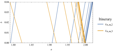
Figure 1: Intersections of $\iota_{\pm,m,n}$-bifurcation parameters. The positive-slope and negative-slope curves are the $\iota_{\pm,m,2}$- and $\iota_{\pm,m,3}$-bifurcation parameters respectively. For each $n$, the curves from left to right are the ones with $m=4,5,\cdots,14$ in ascending order. For each $m$, the two curves have a unique intersection.

Nevertheless, we still can find some patterns of the bifurcation order from the renormalization model. If we fix the value $m$, we showed in the main theorem and Figure 1 that the bifurcation curves $l_{m,2}$ and $l_{m,3}$ intersect. Instead, if we fix the value $n$, we see that the bifurcation curves of $\{\iota_{\pm,m,n}\}_{m=n+1}^{\infty}$ do not intersect. See Figure 2. This suggests that there might be a generalization of the forcing relation that holds for some types of orbits. For example, Misiurewicz and Štimac [MŠ16] used countable many kneading sequences to describe all possible itineraries of an orientation reversing Lozi map.

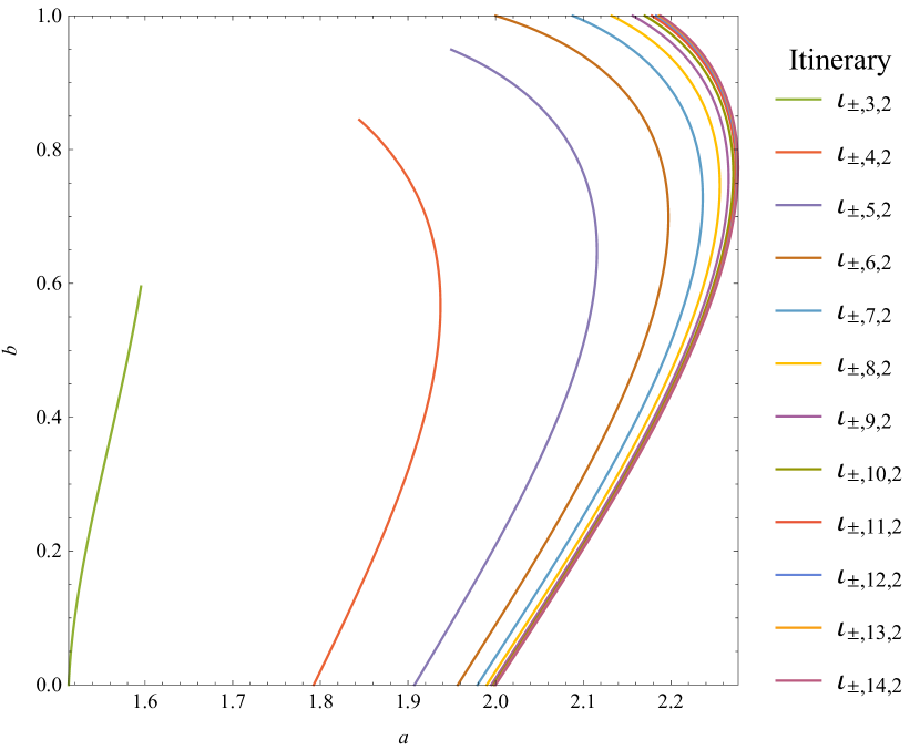
(a) The $\iota_{\pm,m,2}$-bifurcation parameters. The curves are the bifurcation parameters with $m=3,5,\cdots,14$ from left to right.

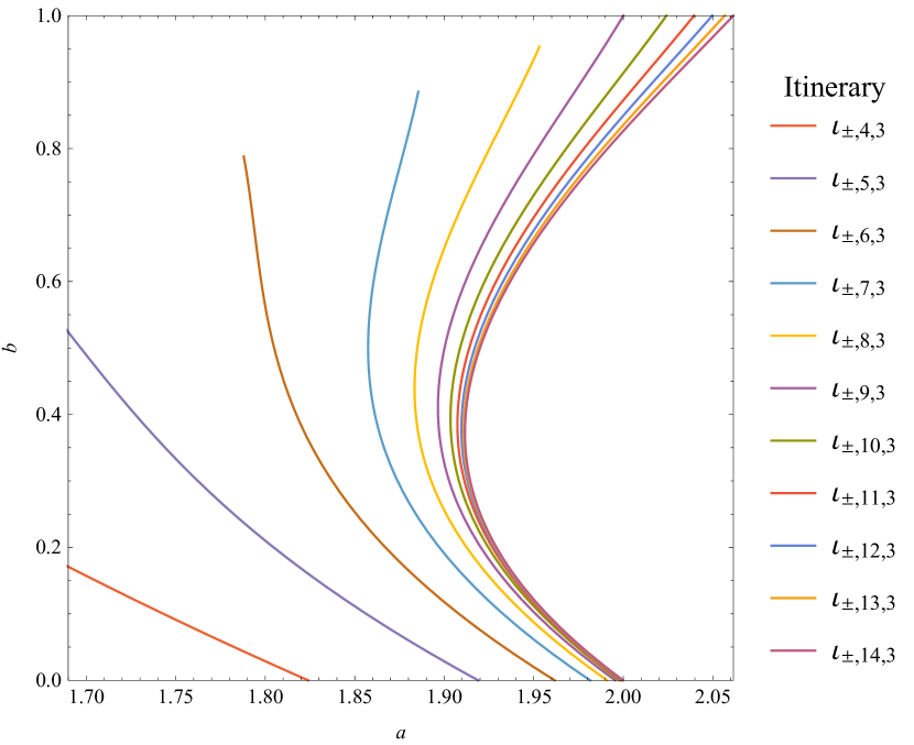
(b) The $\iota_{\pm,m,3}$-bifurcation parameters. The curves are the bifurcation parameters with $m=4,5,\cdots,14$ from left to right.

Figure 2: No intersection of bifurcation parameters.

2 The renormalization model

Recall that the Lozi family is a two-parameter family of maps $\boldsymbol{\Lambda}(x,y)=(-a|x|-by+(a-b-1),x)$, where $a,b\in\mathbb{R}$ are the parameters. The map is expressed as $\boldsymbol{\Lambda}_{a,b}$ if we want to emphasize the Lozi map at a particular parameter $(a,b)$. Let $S=\{-1,+1\}$, $\sigma\in S$, and $\mathbb{R}_{\sigma}=\sigma[0,\infty)$. For simplicity, we may write $-$ and $+$ for the elements of $S$. Denote the $\sigma$-affine branch of $\boldsymbol{\Lambda}$ by $\boldsymbol{\Lambda}_{\sigma}(x,y)=(-\sigma ax-by+(a-b-1),x)$. Let $P_{\operatorname{full}}=\{(a,b);a>b+1\text{ and }0\leq b\leq 1\}$ be a space of parameters. Consider the original family $\widehat{\boldsymbol{\Lambda}}_{a,b}(x,y)=(-a|x|+y+1,bx)$ introduced by Lozi [Loz78]. For all $(a,b)\in P_{\operatorname{full}}$, we have the semi-conjugation $\boldsymbol{H}\circ\boldsymbol{\Lambda}_{a,b}=\widehat{\boldsymbol{\Lambda}}_{a,-b}\circ\boldsymbol{H}$, where $\boldsymbol{H}(x,y)=(\frac{x}{a-b-1},\frac{by}{a-b-1})$. The map $\boldsymbol{H}$ becomes a conjugacy map when $b\neq 0$.

When $(a,b)\in P_{\operatorname{full}}$, the map has two saddle fixed points $\boldsymbol{z}_{-}=(\zeta_{-},\zeta_{-})$ and $\boldsymbol{z}_{+}=(\zeta_{+},\zeta_{+})$, where $\zeta_{-}=-1$ and $\zeta_{+}=1-\frac{2(b+1)}{a+b+1}$. The stable and unstable multipliers of $\boldsymbol{z}_{\sigma}$ are $-\sigma\mu$ and $-\sigma\lambda$, with contracting and expanding directions $(-\sigma\mu,1)$ and $(-\sigma\lambda,1)$ respectively, where $\lambda=\frac{a+\sqrt{a^{2}-4b}}{2}$ and $\mu=\frac{b}{\lambda}$. The stable $W^{S}(\boldsymbol{v})$ and unstable $W^{U}(\boldsymbol{v})$ sets of a periodic point $\boldsymbol{v}$ are unions of connected line segments. We still call them stable and unstable manifolds, even though they are not differentiable manifolds. For $d\in\{S,U\}$, let $W_{0}^{d}(\boldsymbol{v})$ be the line segment of $W^{d}(\boldsymbol{v})$ containing $\boldsymbol{v}$.

Lemma 2.1.

If $(a,b)\in P_{\operatorname{full}}$, then $\lambda>1$ and $0\leq\mu<1$.

Here, we introduce vertical segments and vertical strips to study the geometry of a Lozi map. A line segment $\alpha$ is called a vertical segment on an interval $I^{V}$ if there exists an affine map $h_{\alpha}\mathrel{\mathop{\mathchar 58\relax}}I^{V}\rightarrow\mathbb{R}$ such that $\alpha\cap(\mathbb{R}\times I^{V})=\{(h_{\alpha}(y),y);y\in I^{V}\}$. The vertical slope of $\alpha$ is the slope of $h_{\alpha}$. Suppose that $\alpha$ and $\beta$ are disjoint vertical segments on the interval $I^{V}$. The vertical strip $V(\alpha,\beta)\subset\mathbb{R}\times I^{V}$ is the region bounded between $\alpha$ and $\beta$, including the boundaries $\alpha$ and $\beta$.

We define pullbacks of a vertical segment on $\mathbb{R}\times I^{V}$, where $I^{V}$ is an interval with $0\in\operatornamewithlimits{Interior}(I^{V})$. The image $\boldsymbol{\Lambda}(\mathbb{R}\times I^{V})$ is folded along the $x$-axis. Let $(u^{L},0)$ and $(u^{R},0)$ be the left and right boundary turning points of $\boldsymbol{\Lambda}(\mathbb{R}\times I^{V})$ respectively. Suppose that $\omega$ is a vertical segment and it intersects the $x$-axis at $(w,0)$. Let $L(\omega)$ be the line containing $\omega$. If $u^{L}\geq w$ and $L(\omega)\cap\boldsymbol{\Lambda}(\mathbb{R}\times I^{V})\subset\mathbb{R}\times I^{V}$, then $\boldsymbol{\Lambda}^{-1}(\omega)\cap(\mathbb{R}\times I^{V})$ contains two vertical segments: one is $\Pi_{-}(\omega)$ and the other is $\Pi_{+}(\omega)$, where $\Pi_{\sigma}(\omega)=\boldsymbol{\Lambda}_{\sigma}^{-1}(\omega)\cap(\mathbb{R}\times I^{V})$. See Proposition 2.5 for details. Thus, the transformations $\Pi_{-}$ and $\Pi_{+}$ define pullbacks of a vertical segment by the two branches of $\boldsymbol{\Lambda}$.

We define vertical strips on $\mathbb{R}\times I^{V}$. We consider only the orientation preserving case in this paper, i.e. $b\geq 0$. Let $I^{V}=[-1,1]$. Suppose that $W_{0}^{S}(\boldsymbol{z}_{-})$ and $W_{0}^{S}(\boldsymbol{z}_{+})$ are vertical segments on $I^{V}$. Let $\beta_{1}=W_{0}^{S}(\boldsymbol{z}_{+})\cap(\mathbb{R}\times I^{V})$, $\beta_{m}=\Pi_{-}(\beta_{m-1})$ for $2\leq m<\infty$, $\beta_{\infty}=W_{0}^{S}(\boldsymbol{z}_{-})\cap(\mathbb{R}\times I^{V})$, $\gamma_{m}=\Pi_{+}(\beta_{m})$ for $1\leq m<\infty$, and $\gamma_{\infty}=\Pi_{+}(\beta_{\infty})$. Also, for $1\leq m\leq\infty$, let $(r_{m},0)$ be the intersection point of $\gamma_{m}$ and the $x$-axis. Note that $\beta_{1}=\gamma_{1}$. The vertical segments $\{\beta_{m}\}_{1\leq m<\infty}$ and $\{\gamma_{m}\}_{1\leq m<\infty}$ are subsets of $W^{S}(\boldsymbol{z}_{+})$, while $\beta_{\infty}$ and $\gamma_{\infty}$ are subsets of $W^{S}(\boldsymbol{z}_{-})$. Let $B=V(\beta_{2},\beta_{1})$, $C=V(\gamma_{1},\gamma_{\infty})$, $C^{+}=\{(x,y)\in\mathbb{R}\times I^{V};\gamma_{\infty}(y)\leq x\}$, $C_{m}=V(\gamma_{m-1},\gamma_{m})$ for $2\leq m<\infty$, and $D=V(\beta_{\infty},\gamma_{\infty})$. See Figure 3 for an illustration. The sets $\{C_{m}\}_{2\leq m<\infty}$ form a partition of $C$.

(a) The $\beta$ and $\gamma$ stable manifolds.

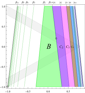
(b) The sets $B$ and $C_{m}$.

Figure 3: The renormalization model of the Lozi map with $(a,b)=(1.8,0.2)$.

In this paper, we center on the renormalization model defined by this partition. Let $P_{\operatorname{mod}}=\{(a,b);a>3b+1\text{ and }0\leq b\leq 1\}$. We show that the renormalization model exists when $(a,b)\in P_{\operatorname{mod}}$.

Lemma 2.2.

We have

$$2b+1<\lambda\leq a$$

for all $(a,b)\in P_{\operatorname{mod}}$.

Lemma 2.3.

If $(a,b)\in P_{\operatorname{mod}}$, then $\beta_{\infty}$ and $\gamma_{\infty}$ exist.

Moreover, let $L=[\beta_{\infty}(\min I^{V}),\gamma_{\infty}(\min I^{V})]\times\{\min I^{V}\}$, $K=[\beta_{\infty}(\max I^{V}),\gamma_{\infty}(\max I^{V})]\times\{\max I^{V}\}$, $L_{\sigma}=L\cap(\mathbb{R}_{\sigma}\times\mathbb{R})$, and $K_{\sigma}=K\cap(\mathbb{R}_{\sigma}\times\mathbb{R})$ for $\sigma\in S$. For each $J\in\{K,L\}$, $\boldsymbol{\Lambda}(J)$ is the union of two line segments $\boldsymbol{\Lambda}(J)=\boldsymbol{\Lambda}_{-}(J_{-})\cup\boldsymbol{\Lambda}_{+}(J_{+})$. The segment $\boldsymbol{\Lambda}_{+}(J_{+})$ is located on the upper half plan; while the segment $\boldsymbol{\Lambda}_{-}(J_{-})$ is located on the lower half plan. The left ends of the segments are on $\beta_{\infty}$ and the right ends of the segments are on the $x$-axis.

Proof.

Let $v_{-}=-1+\frac{2b}{\lambda}$, $\boldsymbol{V}_{-}=(v_{-},1)$, and $\boldsymbol{W}_{-}=z_{-}$. Clearly, $\boldsymbol{V}_{-},\boldsymbol{W}_{-}\in L(W_{0}^{S}(\boldsymbol{z}_{-}))$. By Lemma 2.2, we have

$$v_{-}<-1+\frac{2b}{2b+1}<0.$$

Thus, $\beta_{\infty}$ exists and $\beta_{\infty}=\overline{\boldsymbol{V}_{-}\boldsymbol{W}_{-}}$.

Let $v_{+}=1-\frac{2\lambda+2}{a\lambda+b}b$, $w_{+}=1-\frac{2}{a\lambda+b}b$, $\boldsymbol{V}_{+}=(v_{+},1)$, and $\boldsymbol{W}_{+}=(w_{+},-1)$. By Lemma 2.2 and the inequality of arithmetic and geometric means, we have

$$v_{+}=1-\frac{2b(\lambda+1)}{\lambda^{2}+2b}\geq 1-\frac{2b(\lambda+1)}{\lambda^{2}}\geq 1-\frac{2b(2b+2)}{(2b+1)^{2}}\geq 0.$$

Clearly, $v_{+}\leq w_{+}\leq 1$ and hence $\boldsymbol{\Lambda}(\boldsymbol{V}_{+}),\boldsymbol{\Lambda}(\boldsymbol{W}_{+})\in\beta_{\infty}$. Thus, $\gamma_{\infty}$ exists and $\gamma_{\infty}=\overline{\boldsymbol{V}_{+}\boldsymbol{W}_{+}}$.

Finally, by definition, we have $K=\overline{\boldsymbol{V}_{-}\boldsymbol{V}_{+}}$, $L=\overline{\boldsymbol{W}_{-}\boldsymbol{W}_{+}}$, and $\boldsymbol{\Lambda}(\boldsymbol{V}_{-}),\boldsymbol{\Lambda}(\boldsymbol{V}_{+}),\boldsymbol{\Lambda}(\boldsymbol{W}_{-}),\boldsymbol{\Lambda}(\boldsymbol{W}_{+})\in\beta_{\infty}$. This completes the proof. ∎

Corollary 2.4.

Let $(a,b)\in P_{\operatorname{mod}}$. Then $\boldsymbol{\Lambda}(D)\subset\{(x,y)\in\mathbb{R}\times I^{V};x\geq\beta_{\infty}(y)\}$.

Proof.

The corollary follows immediately from Lemma 2.3. ∎

Proposition 2.5.

Let $(a,b)\in P_{\operatorname{mod}}$, $\omega\subset D$ be a vertical segment on $I^{V}$, and $(w,0)$ be the intersection point of $\omega$ and the $x$-axis. If $w\leq u^{L}$, then $\Pi_{\sigma}(\omega)\subset D\cap(\mathbb{R}_{\sigma}\times\mathbb{R})$ is a vertical segment on $I^{V}$ for each $\sigma\in S$. We have $\boldsymbol{\Lambda}^{-1}(\omega)\cap(\mathbb{R}\times I^{V})=\Pi_{-}(\omega)\cup\Pi_{+}(\omega)$.

Proof.

Let $K_{\sigma}$ and $L_{\sigma}$ be the line segments defined in Lemma 2.3. If $w\leq u^{L}$, then $\omega$ and $\boldsymbol{\Lambda}(J_{\sigma})$ have a unique intersection point on $\mathbb{R}\times\mathbb{R}_{\sigma}$ for $J\in\{K,L\}$ by Lemma 2.3. The preimage $\boldsymbol{\Lambda}^{-1}(\omega\cap(\mathbb{R}\times\mathbb{R}_{\sigma}))$ is a line segment connecting $K_{\sigma}$ and $L_{\sigma}$. Thus, $\Pi_{\sigma}(\omega)$ is a vertical segment on $I^{V}$ and $\Pi_{\sigma}(\omega)=\boldsymbol{\Lambda}^{-1}(\omega)\cap(\mathbb{R}_{\sigma}\times I^{V})\subset D\cap(\mathbb{R}_{\sigma}\times\mathbb{R})$. ∎

Lemma 2.6.

If $(a,b)\in P_{\operatorname{mod}}$, then $\beta_{1}=\gamma_{1}$ exists and $r_{1}<u^{L}$.

Proof.

Clearly, $\beta_{1}=\{\zeta_{+}\}\times I^{V}$ when $b=0$. When $b>0$, $W_{0}^{S}(\boldsymbol{z}_{+})$ is the line segment from $(0,v_{1})$ to $(v_{1},v_{2})$ where $v_{1}=(1+\frac{\lambda}{b})\zeta_{+}$ and $v_{2}=[1-(\frac{\lambda}{b})^{2}]\zeta_{+}$. Note that $\zeta_{+}=\frac{(\lambda-1)(\lambda-b)}{(\lambda+1)(\lambda+b)}$. By Lemma 2.2, we get

$$v_{1}=\frac{\lambda-1}{b}\frac{\lambda-b}{\lambda+1}>\frac{2b}{b}\frac{b+1}{2b+2}=\max I^{V}.$$

Also, by Lemma 2.2, we get

$$v_{2}=-\frac{\lambda-1}{b}\frac{\lambda-b}{b}\frac{\lambda-b}{\lambda+1}<-\frac{2b}{b}\frac{b+1}{b}\frac{b+1}{2b+2}<\min I^{V}.$$

Thus, $\beta_{1}$ exist.

Moreover, by definition, we have $u^{L}=a-2b-1$ and $r_{1}=(1+\frac{b}{\lambda})\zeta_{+}$. By Lemma 2.2, we get

$$u^{L}-r_{1}=\frac{\lambda}{\lambda+1}(\lambda-2b-1)>0.\qed$$

Theorem 2.7.

If $(a,b)\in P_{\operatorname{mod}}$, then the renormalization model exists.

Proof.

The vertical segments $\beta_{\infty}$ and $\gamma_{\infty}$ exist by Lemma 2.3.

We claim that $\beta_{m}$ exists and $w_{m}\leq u^{L}$ by induction on $m\geq 1$, where $(w_{m},0)$ is the intersection point of $\beta_{m}$ and the $x$-axis. The base case follows from Lemma 2.6. Suppose that $\beta_{m}$ is a vertical segment and $w_{m}\leq u^{L}$ for some $m\geq 1$. By Proposition 2.5, $\beta_{m+1}=\Pi_{-}(\beta_{m})$ exists and $w_{m+1}\leq 0\leq u^{L}$. Consequently, this proves the claim by induction.

By Proposition 2.5, $\gamma_{m}=\Pi_{+}(\beta_{m})$ exists because $w_{m}\leq u^{L}$. This completes the proof. ∎

Remark 2.8.

By choosing a different $I^{V}$, we can show that the renormalization model exists on $\{(a,b);a>3|b|+1\text{ and }-1\leq b\leq 1\}$.

Next, we study the orbit of $C_{m}$. Let $B_{m}=\boldsymbol{\Lambda}^{m-1}(C_{m})$ and $U_{m}=\boldsymbol{\Lambda}(B_{m})$. See Figures 4 and 5 for illustrations. By the definition of the vertical segments, we have $B_{m}\subset B$ for all $m$. The pieces $\{B_{m}\}_{2\leq m<\infty}$ converge to $W_{0}^{U}(\boldsymbol{z}_{-})$ exponentially. The $m$-th iterate $U_{m}$ returns to $C$, and is folded along the $x$-axis. Thus, the $m$-fold iterate $\boldsymbol{\Lambda}^{m}\mathrel{\mathop{\mathchar 58\relax}}C_{m}\rightarrow U_{m}$ forms a “Lozi-like map” in a microscopic scale. Let $(u_{m}^{L},0)$ and $(u_{m}^{R},0)$ be the left and right boundary turning points of $U_{m}$ respectively. And let $(u_{\infty},0)$ be the intersection point of $W_{0}^{U}(\boldsymbol{z}_{-})$ and the $x$-axis. The values $u_{m}^{L}$ and $u_{m}^{R}$ serve as the “critical values” of $\boldsymbol{\Lambda}^{m}|_{C_{m}}$. They converge to $u_{\infty}$ exponentially as $m\rightarrow\infty$ when $b>0$, and degenerate to a single value when $b=0$. The position of the critical values govern the dynamics in a microscopic scale. If $r_{m-1}\leq u_{m}^{R}$, then $C_{m}\cap U_{m}\neq\emptyset$, and the orbit of a point in $C_{m}$ may have a recurrence in the set. This is called the renormalization defined by one return to $C$.

Proposition 2.9.

Suppose that $(a,b)\in P_{\operatorname{mod}}$. Then the followings are true.

1. $r_{m}<r_{n}<r_{\infty}$ for all $1\leq m<n$.

2. $u^{L}\leq u_{m}^{L}\leq u_{m}^{R}\leq u_{n}^{L}\leq u_{\infty}\leq u^{R}$ for all $2\leq m<n$.

Proof.

The properties can be proved by using the techniques developed in Sections 5.1 and 5.3. The details are left to the reader. ∎

Remark 2.10.

If the map is orientation reversing and the renormalization model exists, then the order of the turning points will be flipping sides alternatively:

$$u^{L}\leq u_{3}^{L}\leq u_{3}^{R}\leq u_{5}^{L}\leq u_{5}^{R}\leq\cdots\leq u_{\infty}\leq\cdots\leq u_{4}^{L}\leq u_{4}^{R}\leq u_{2}^{L}\leq u_{2}^{R}\leq u^{R}.$$

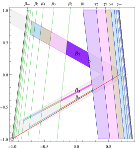
(a) The sets $B_{m}$ on the phase space. The parameters of the map are $(a,b)=(1.8,0.2)$.

(b) The exponential convergence of $B_{m}$.

Figure 4: The sets $B_{m}$.

(a) The sets $U_{m}$ on the phase space. The parameters of the map are $(a,b)=(1.8,0.2)$.

(b) The exponential convergence of $U_{m}$.

Figure 5: The sets $U_{m}$.

Moreover, we define a subpartition $\{C_{m,n}\}_{2\leq n<\infty}$ on $C_{m}$. Let $C_{m,n}=\boldsymbol{\Lambda}^{-m}(U_{m}\cap C_{n})$ for $m,n\geq 2$. See Figure 6 for an illustration.

Proposition 2.11.

Suppose that $(a,b)\in P_{\operatorname{mod}}$ and $m,n\geq 2$. If $r_{n}\leq u_{m}^{L}$, then $C_{m,n}$ is the union of two disjoint vertical strips. The vertical strips are bounded between vertical segments which are subsets of $W^{S}(\boldsymbol{z}_{+})$. Let $C_{m,n}^{L}$ and $C_{m,n}^{R}$ be the left and right components respectively.

Proof.

The proof is similar to Proposition 2.5. The details are left to the reader. ∎

If the conclusion of Proposition 2.11 holds, let $B_{m,n}^{d}=\boldsymbol{\Lambda}^{m+n-1}(C_{m,n}^{d})$ and $U_{m,n}^{d}=\boldsymbol{\Lambda}(B_{m,n}^{d})$ for $d\in\{L,R\}$. We note that $B_{m,n}^{d}\subset B_{n}$ and $U_{m,n}^{d}\subset U_{n}$. The image $\boldsymbol{\Lambda}^{m+n}(C_{m,n}^{d})$ is folded along the $x$-axis. Thus, the $(m+n)$-fold iterate $\boldsymbol{\Lambda}^{m+n}\mathrel{\mathop{\mathchar 58\relax}}C_{m,n}^{d}\rightarrow U_{m,n}^{d}$ forms a “Lozi-like map” in a microscopic scale. If $C_{m,n}^{d}\cap U_{m,n}^{d}\neq\emptyset$, then the orbit of a point in $C_{m,n}^{d}$ may have a recurrence in the set. This is called the renormalization defined by two returns to $C$.

(a) The subpartition, $U_{2}$, and $U_{3}$ on the phase space.

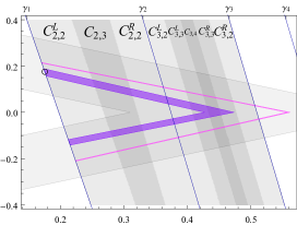
(b) A zoomed view of the subpartition.

Figure 6: The subpartition that establishes the renormalization defined by two returns to $C$. The parameters of the map are $(a,b)=(1.71,0.2)$.

An outline of the proof of the main theorem (Theorem 7.1)

We consider the two pairs of periodic points $\boldsymbol{\theta}_{-,m,2},\boldsymbol{\theta}_{+,m,2}\in C_{m,2}^{L}$ and $\boldsymbol{\theta}_{-,m,3},\boldsymbol{\theta}_{+,m,3}\in C_{m,3}^{L}$ created by the renormalization defined by two returns to $C$. The points depend analytically on the parameters $(a,b)$ whenever they exist (Theorem 3.2). For each pair $(\boldsymbol{\theta}_{-,m,n},\boldsymbol{\theta}_{+,m,n})$, the two periodic points are created when there is a border collision bifurcation [Leo59, NY92]. The bifurcation parameters $(a,b)$ form an analytic curve $a=l_{m,n}(b)$ on the parameter space (Theorem 6.6). The existence of the curve is proved by using a geometrical characterization of the bifurcation given in Proposition 4.3. Our goal is to show that the two curves $l_{m,2}$ and $l_{m,3}$ have a unique intersection and the intersection is transverse.

We consider a curve $a=t(b)$ on the parameter space such that the Lozi map $\boldsymbol{\Lambda}_{a,b}$ has a homoclinic tangency $(r_{\infty},0)=(u_{\infty},0)$ (Proposition 6.8). Both the stable laminations $(r_{m},0)$ and the turning points $(u_{m}^{L,R},0)$ converge exponentially to the homoclinic point as $m\rightarrow\infty$ (Propositions 5.12 and 5.23). Thus, we apply the logarithm coordinate transformation $T(x)=-\log_{\lambda}(r_{\infty}-x)$ to the $x$-coordinate.

Under the coordinate change, the stable laminations $T(r_{m})$ are located on the integral points $m$; while the turning points $T(u_{n}^{L,R})$ are located on $(n-1)\log_{\lambda}b^{-1}$. Since $\lambda$ is bounded on the parameter curve $t$, the estimation $\log_{\lambda}\overline{b}^{-1}\gg 2$ holds when $\overline{b}>0$ is sufficiently small (the condition (7.5)). Thus, when $(a,b)=(t(\overline{b}),\overline{b})$, there exists an integer $m$ such that

$$T(u_{2}^{R})<m-1=T(r_{m-1})<m=T(r_{m})<T(u_{3}^{L}).$$ (2.1)

The geometry of the points is illustrated as in Figure 7.

We show that the order of creation of the pairs $(\boldsymbol{\theta}_{-,m,2},\boldsymbol{\theta}_{+,m,2})$ and $(\boldsymbol{\theta}_{-,m,3},\boldsymbol{\theta}_{+,m,3})$ is opposite on the parameter lines $b=0$ and $b=\overline{b}$ while we vary $a$. On the one hand, when $(a,b)=(t(\overline{b}),\overline{b})$, the relation (2.1) holds. We have $U_{2}\cap C_{m,2}^{L}=\emptyset$ since $T(u_{2}^{R})<T(r_{m-1})$. Thus, $\boldsymbol{\theta}_{-,m,2}$ and $\boldsymbol{\theta}_{+,m,2}$ do not exist. Also, $\boldsymbol{\Lambda}^{m+3}\mathrel{\mathop{\mathchar 58\relax}}C_{m,3}^{L}\rightarrow U_{3}$ forms a full horseshoe since $T(u_{3}^{L})>T(r_{m})$. Thus, $\boldsymbol{\theta}_{-,m,3}$ and $\boldsymbol{\theta}_{+,m,3}$ exist. This shows that $(\boldsymbol{\theta}_{-,m,3},\boldsymbol{\theta}_{+,m,3})$ is created before $(\boldsymbol{\theta}_{-,m,2},\boldsymbol{\theta}_{+,m,2})$ on the line $b=\overline{b}$. On the other hand, when $b=0$, we have $U=U_{2}=U_{3}$. As the parameter $a$ increases, $U$ will first intersects $C_{m,2}^{L}$ then intersects $C_{m,3}^{L}$. This implies that $(\boldsymbol{\theta}_{-,m,2},\boldsymbol{\theta}_{+,m,2})$ is created before $(\boldsymbol{\theta}_{-,m,3},\boldsymbol{\theta}_{+,m,3})$ on the line $b=0$. See also Section 3.4 for the forcing relation in one dimension. Therefore, the order of creation is opposite, and hence $l_{m,2}$ and $l_{m,3}$ has an intersection.

Moreover, the intersection is unique and transverse because $\frac{\operatorname{d\!}l_{m,2}}{\operatorname{d\!}b}>\frac{\operatorname{d\!}l_{m,3}}{\operatorname{d\!}b}$ when $b$ is small (Corollary 6.7).

Figure 7: The configuration of a Lozi map when the order of bifurcation is reversed.

3 Symbolic dynamics and formal periodic orbits

We consider periodic orbits obtained from the two affine branches $\boldsymbol{\Lambda}_{-}$ and $\boldsymbol{\Lambda}_{+}$. They are candidates of the periodic orbits of the Lozi map. An itinerary $I=(I_{1},\cdots,I_{l(I)})$ is a sequence of alphabets in $S$ with a length $l(I)\in\{1,\cdots,\infty\}$. An itinerary $I$ is finite if $l(I)<\infty$. When $I$ and $J$ are itineraries and $I$ is finite, we write $IJ$ for the concatenation of $I$ and $J$, $I*$ for itineraries that start with $I$ and end with any tail, and $I^{\infty}=II\cdots$. When $I$ is a finite itinerary, we write $\boldsymbol{\Lambda}_{I}=\boldsymbol{\Lambda}_{I_{N}}\circ\cdots\circ\boldsymbol{\Lambda}_{I_{1}}$, where $N=l(I)$. The formal $I$-orbit $O_{I}(\boldsymbol{\theta})$ of $\boldsymbol{\theta}\in\mathbb{R}^{2}$ is the sequence $\{\boldsymbol{\theta}_{m}\in\mathbb{R}^{2}\}_{m=0}^{l(I)}$ such that $\boldsymbol{\theta}_{0}=\boldsymbol{\theta}$ and

$$\boldsymbol{\theta}_{m}=\boldsymbol{\Lambda}_{(I_{1},\cdots,I_{m})}(\boldsymbol{\theta})$$

for $1\leq m\leq l(I)$. A point $\boldsymbol{\theta}\in\mathbb{R}^{2}$ is a formal $I$-periodic point if $I$ is finite and

$$\boldsymbol{\theta}=\boldsymbol{\Lambda}_{I}(\boldsymbol{\theta}).$$ (3.1)

Its formal $I$-orbit is called a formal $I$-periodic orbit.

Next, we introduce the notion of admissibility. Let $\boldsymbol{\theta}$ be a point and $I$ be an itinerary. Let $\pi_{1}(x,y)=x$ and $\pi_{2}(x,y)=y$. The point $\boldsymbol{\theta}$ is $I$-admissible if $\pi_{1}(\boldsymbol{\theta})\in\mathbb{R}_{I_{1}}$ and $\pi_{1}\circ\boldsymbol{\Lambda}_{(I_{1},\cdots,I_{m-1})}(\boldsymbol{\theta})\in\mathbb{R}_{I_{m}}$ for $m=2,\cdots,l(I)$. When $I$ is finite, the $I$-admissibility function is defined as

$$h_{I}(a,b,\boldsymbol{\theta})=\min\{I_{1}\pi_{1}(\boldsymbol{\theta}),I_{2}\pi_{1}\circ\boldsymbol{\Lambda}_{(I_{1})}(\boldsymbol{\theta}),\cdots,I_{M}\pi_{1}\circ\boldsymbol{\Lambda}_{(I_{1},\cdots,I_{M-1})}(\boldsymbol{\theta})\},$$ (3.2)

where $M=l(I)$. Thus, a point $\boldsymbol{\theta}$ is $I$-admissible at a parameter $(a,b)$ if and only if $h_{I}(a,b,\boldsymbol{\theta})\geq 0$. If $\boldsymbol{\theta}$ is $I$-admissible, then $\boldsymbol{\Lambda}_{(I_{1},\cdots,I_{m})}(\boldsymbol{\theta})=\boldsymbol{\Lambda}^{m}(\boldsymbol{\theta})$ for $m=1,\cdots,l(I)$. Thus, admissible formal periodic points are periodic points of the Lozi map. We will show that for any given itinerary $s$, there exists a unique formal $I$-periodic point.

3.1 Existence and uniqueness of formal periodic orbits

To prove the existence of a formal periodic point, we write $\boldsymbol{\Lambda}_{I}(\boldsymbol{\theta})=\boldsymbol{A}\boldsymbol{\theta}-\boldsymbol{w}$, where $I$ is a finite itinerary, $\boldsymbol{A}\equiv\operatorname{D\!}\boldsymbol{\Lambda}_{I}$ is the linear term of the affine map $\boldsymbol{\Lambda}_{I}$, and $\boldsymbol{w}$ is a vectored-polynomial in $a$ and $b$. Then (3.1) can be rewritten as a linear equation

$$(\boldsymbol{A}-\operatorname{Id})\boldsymbol{\theta}=\boldsymbol{w}.$$ (3.3)

If the eigenvalues of $\boldsymbol{A}$ are not $1$, then (3.3) has a unique solution, which yields the desired periodic point. To ensure that the spectrum of $\boldsymbol{\Lambda}_{-}$ is away from $1$, we restrict our parameters to $P_{\operatorname{full}}$ in this section.

Lemma 3.1.

Suppose that $(a,b)\in P_{\operatorname{full}}$. A lower bound of the spectral radius $\rho(\operatorname{D\!}\boldsymbol{\Lambda}_{I})$ is provided by

$$\rho(\operatorname{D\!}\boldsymbol{\Lambda}_{I})\geq\lambda^{l(I)}.$$

Proof.

By the expansion of the universal unstable cone (Theorem A.1), we have

$$\left\|(\operatorname{D\!}\boldsymbol{\Lambda}_{I})^{m}\right\|_{2}\geq\lambda^{l(I)m}$$

for all $m\geq 0$ where the norm is the $L^{2}$ operator norm. Thus, the lemma follows from the Gelfand’s formula [Lax02, P. 159]. ∎

Finally, by using the fact that the spectrum is away from $1$, this gives a new proof of the existence and uniqueness of a formal periodic point.

Theorem 3.2.

Suppose that $(a,b)\in P_{\operatorname{full}}$. For each finite itinerary $I$, there exists a unique $I$-formal periodic point $\boldsymbol{\theta}$. The point $\boldsymbol{\theta}$ is a saddle fixed point of $\boldsymbol{\Lambda}_{I}$. In fact, consider the formal periodic point as a map $\boldsymbol{\theta}\mathrel{\mathop{\mathchar 58\relax}}P_{\operatorname{full}}\rightarrow\mathbb{R}^{2}$, the maps $\pi_{1}\circ\boldsymbol{\theta}$ and $\pi_{2}\circ\boldsymbol{\theta}$ are rational functions in $a$ and $b$.

Proof.

Let $\nu_{1}$ and $\nu_{2}$ be the eigenvalues of $\boldsymbol{A}$. Without loss of generality, we assume that $|\nu_{1}|=\rho(\boldsymbol{A})$. By Lemma 2.1, Corollary 3.1, and $\det(\operatorname{D\!}\boldsymbol{\Lambda}_{\sigma})=b$ for $\sigma\in S$, we get $|\nu_{1}|\geq\lambda^{M}>1$ and $|\nu_{2}|\leq\mu^{M}<1$ where $M=l(I)$. Thus, (3.3) has a unique solution $\boldsymbol{\theta}$, and $\boldsymbol{\theta}$ is a saddle fixed point of $\boldsymbol{\Lambda}_{I}$. The solution is a rational function because the entries of $\boldsymbol{A}$ and $\boldsymbol{w}$ are polynomials in $a$ and $b$. ∎

Remark 3.3.

Let $\hat{\lambda}=\frac{a+\sqrt{a^{2}-4|b|}}{2}$. By the existence of the universal unstable cone, $\hat{\lambda}>1$, and $\frac{|b|}{\hat{\lambda}}<1$, the theorem can be generalized to the parameter space $\{(a,b);a>|b|+1\}$.

It follows immediately by the theorem and Theorem B.1 that formal periodic points are the only candidates having periodic itineraries.

Corollary 3.4.

Suppose that $(a,b)\in P_{\operatorname{full}}$ and $I$ is a finite itinerary. If $\boldsymbol{\Lambda}$ has a $I^{\infty}$-admissible point $\boldsymbol{v}\in\mathbb{R}^{2}$, then exactly one of the following holds.

1. If $\boldsymbol{v}$ has unbounded orbit, then $I^{\infty}=(-)^{\infty}$ and $\lim_{m\rightarrow\infty}\pi_{1}\circ\boldsymbol{\Lambda}^{m}(\boldsymbol{v})=-\infty$.

2. If $\boldsymbol{v}$ has bounded orbit, then $\boldsymbol{v}$ is the formal $I$-periodic point.

3.2 Hyperbolicity and the border collision bifurcation

A formal $I$-periodic point $\boldsymbol{\theta}$ is called hyperbolic if it is $I$-admissible and $\pi_{1}\circ\boldsymbol{\Lambda}^{m}(\boldsymbol{\theta})\neq 0$ for all $0\leq m<l(I)$. It is hyperbolic at a parameter $(a,b)$ if and only if $h_{I}(a,b,\boldsymbol{\theta}(a,b))>0$. Thus, a hyperbolic formal $I$-periodic point persists under a small perturbation of a parameter.

Suppose that a formal $I$-periodic point $\boldsymbol{\theta}$ is admissible and $\pi_{1}\circ\boldsymbol{\Lambda}^{m}(\boldsymbol{\theta})=0$ for some $m\geq 0$ at a parameter $(a_{0},b_{0})$. This is exactly the case when $h_{I}(a_{0},b_{0},\boldsymbol{\theta}(a_{0},b_{0}))=0$. Without lose of generality, we may assume that $m=0$. Then $\boldsymbol{\theta}$ is simultaneously $(-,I_{2},\cdots,I_{M})$- and $(+,I_{2},\cdots,I_{M})$-admissible at $(a_{0},b_{0})$ where $M=l(I)$. After applying a small perturbation to the parameter $(a_{0},b_{0})$, there may be a creation (or annihilation) of two periodic orbits, each satisfying one of the itineraries. This is called the border collision bifurcation [Leo59, NY92]. The parameter $(a_{0},b_{0})$ is called a bifurcation parameter of the itineraries $(\pm,I_{2},\cdots,I_{M})$.

3.3 Symbolic dynamics on the renormalization model

In this section, we apply symbolic dynamics to periodic orbits created by the renormalization defined by two returns to $C$. We find the coding of periodic orbits in $C_{m,n}^{L}$. Recall that $\iota_{\sigma,m,n}=(+(-)^{m-2}++(-)^{n-2}\sigma)$ and $\boldsymbol{\theta}_{\sigma,m.n}$ is the formal $\iota_{\sigma,m,n}$-periodic point for $\sigma\in S$ and $m,n\geq 2$.

Proposition 3.5.

Suppose that $(a,b)\in P_{\operatorname{mod}}$, $m,n\geq 2$, and $C_{m,n}^{L}$ exists at $(a,b)$. If $\boldsymbol{v}\in C_{m,n}^{L}$, then $\boldsymbol{v}$ is either $\iota_{-,m,n}$- or $\iota_{+,m,n}$-admissible and $\pi_{1}\circ\boldsymbol{\Lambda}^{j}(\boldsymbol{v})\neq 0$ for all $j\in\{1,\cdots,m-2,m,\cdots,m+n-2\}$. In addition, if $\boldsymbol{v}$ is a periodic point, then $\pi_{1}\circ\boldsymbol{\Lambda}^{j}(\boldsymbol{v})\neq 0$ for $j\in\{0,\cdots,m+n-2\}$.

Conversely, if the formal $\iota_{\sigma,m,n}$-periodic point is admissible, we show that the point is constraint in $C_{m,n}^{L}$.

Lemma 3.6.

Suppose that $(a,b)\in P_{\operatorname{mod}}$ and $m\geq 3$. Let $I=(+(-)^{m-2}+)$. If $\boldsymbol{v}\in\mathbb{R}\times I^{V}$ is $I$-admissible, then one of the following is true.

1. $\boldsymbol{v}\in C_{m}$ and $\boldsymbol{\Lambda}^{m-1}(\boldsymbol{v})\in B$.

2. $\boldsymbol{v}\in C_{m-1}$ and $\boldsymbol{\Lambda}^{m-1}(\boldsymbol{v})\in C\cup C^{+}$.

Proof.

Let $A^{-}=\{(x,y)\in\mathbb{R}\times I^{v};x\leq\beta(y)\}$ and $A_{m}=V(\beta_{m},\beta_{m-1})$ for $m\geq 2$. By definition, $\boldsymbol{\Lambda}^{m-2}(\boldsymbol{v})\in\mathbb{R}_{-}\times I^{V}\subset A^{-}\cup(\cup_{m=2}^{\infty}A_{m})$. Since $\boldsymbol{\Lambda}(A^{-}),\boldsymbol{\Lambda}(A_{n})\subset(-\infty,0)\times\mathbb{R}$ for all $n\geq 4$, we have $\boldsymbol{\Lambda}^{m-2}(\boldsymbol{v})\in A_{2}\cup A_{3}$. This proves the lemma. ∎

Lemma 3.7.

Suppose that $(a,b)\in P_{\operatorname{mod}}$. If $\boldsymbol{v}\in\mathbb{R}\times I^{V}$ is $(++)$-admissible, then one of the following is true.

1. $\boldsymbol{v}\in B$ and $\boldsymbol{\Lambda}(\boldsymbol{v})\in C\cup C^{+}$.

2. $\boldsymbol{v}\in C_{2}$ and $\boldsymbol{\Lambda}(\boldsymbol{v})\in B$.

Proof.

By definition, $\mathbb{R}_{+}\times I^{V}\subset B\cup(\cup_{m=2}^{\infty}C_{m})\cup C^{+}$. Since $\boldsymbol{\Lambda}(C_{m}),\boldsymbol{\Lambda}(C^{+})\subset(-\infty,0)\times I^{V}$ for all $m\geq 3$, the lemma follows. ∎

Corollary 3.8.

Suppose that $(a,b)\in P_{\operatorname{mod}}$ and $m\geq 3$. Let $I=(+(-)^{m-2}++)$. If $\boldsymbol{v}\in\mathbb{R}\times I^{V}$ is $I$-admissible, then one of the following is true.

1. $\boldsymbol{v}\in C_{m}$ and $\boldsymbol{\Lambda}^{m}(\boldsymbol{v})\in C\cup C^{+}$.

2. $\boldsymbol{v}\in C_{m-1}$ and $\boldsymbol{\Lambda}^{m}(\boldsymbol{v})\in B$.

Proposition 3.9.

Suppose that $(a,b)\in P_{\operatorname{mod}}$, $\sigma\in S$, $m\geq 3$, and $n\geq 2$. If $\boldsymbol{\theta}_{\sigma,m,n}$ is admissible, then $\boldsymbol{\theta}_{\sigma,m,n}\in C_{m}$ and $\boldsymbol{\Lambda}^{m}(\boldsymbol{\theta}_{\sigma,m,n})\in C_{n}$.

Proof.

By Corollary B.2, we have $\boldsymbol{\theta}_{\sigma,m,n}\in D\subset\mathbb{R}\times I^{V}$. Also, $\boldsymbol{\theta}_{\sigma,m,n}\notin W^{S}(\boldsymbol{z}_{+})$ by assumption.

First, consider the case $n=2$. By Lemma 3.6, we have $\boldsymbol{\Lambda}^{m+2}(\boldsymbol{\theta}_{\sigma})=\boldsymbol{\theta}\in C$. This forces $\boldsymbol{\Lambda}^{m+1}(\boldsymbol{\theta}_{\sigma,m,n})\in B$. Thus, $\boldsymbol{\theta}_{\sigma,m,n}\in C_{m}$ and $\boldsymbol{\Lambda}^{m}(\boldsymbol{\theta}_{\sigma,m,n})\in C_{2}$ by Corollary 3.8.

Now, assume that $n\geq 3$. Then $\boldsymbol{\Lambda}^{m}(\boldsymbol{\theta}_{\sigma,m,n})$ is $(+(-)^{n-1}+)$-admissible if $\boldsymbol{\theta}_{\sigma,m,n}$ is $\iota_{-,m,n}$-admissible, or $(+(-)^{n-2}+)$-admissible if $\boldsymbol{\theta}_{\sigma,m,n}$ is $\iota_{+,m,n}$-admissible. By Lemma 3.6, we get $\boldsymbol{\Lambda}^{m}(\boldsymbol{\theta}_{\sigma,m,n})\in C_{n-1}\cup C_{n}\cup C_{n+1}\subset C$. This forces $\boldsymbol{\theta}_{\sigma,m,n}\in C_{m}$ by Corollary 3.8. We obtain $\boldsymbol{\Lambda}^{m}(\boldsymbol{\theta}_{\sigma,m,n})\in C_{n}$ because $\boldsymbol{\Lambda}^{m+n}(\boldsymbol{\theta}_{\sigma,m,n})=\boldsymbol{\theta}_{\sigma,m,n}$. ∎

Corollary 3.10.

Suppose that $(a,b)\in P_{\operatorname{mod}}$, $\sigma\in S$, $m\geq 3$, $n\geq 2$, and $C_{m,n}^{L}$ exists. Then $\boldsymbol{v}\in\mathbb{R}^{2}$ is the admissible formal $\iota_{\sigma,m,n}$-periodic point if and only if $\boldsymbol{v}\in C_{m,n}^{L}$ is a periodic point with period $m+n$.

Proof.

By Proposition 3.9, we have $\boldsymbol{\theta}_{\sigma,m,n}\in C_{m,n}$. Since $C_{m,n}^{L}$ exists, we have $C_{m,n}=C_{m,n}^{L}\cup C_{m,n}^{R}$. Note that $\boldsymbol{\Lambda}^{m-1}(C_{m,n}^{R})\backslash W^{S}(\boldsymbol{z}_{+})\subset(-\infty,0)\times I^{V}$ and $\boldsymbol{\theta}_{\sigma,m,n}\notin W^{S}(\boldsymbol{z}_{+})$. Therefore, $\boldsymbol{\theta}_{\sigma,m,n}\in C_{m,n}^{L}$.

The converse follows immediately from Proposition 3.5. ∎

3.4 The forcing relation from the kneading theory

For completeness, we give a brief review of the forcing relation on itineraries for unimodal maps. The materials are based on [CE80]. We explain why Theorem 7.1 gives a counterexample to the one-dimensional forcing relation. The remaining part of this paper is independent of this section.

A continuous map $f\mathrel{\mathop{\mathchar 58\relax}}[-1,1]\rightarrow[-1,1]$ is unimodal if it has a unique maximum point $c\in(-1,1)$ such that $f(c)=1$, $f(1)=-1$, and $f$ is monotone on each component of $[-1,1]\backslash\{c\}$. Let $I$ be an itinerary. A point $x$ (or orbit $O(x)$) is $I$-admissible if $I_{m}(f^{m-1}(x)-c)\geq 0$ for $m\in\{1,\cdots,l(I)\}$. Here, the critical point is allowed to be encoded as either “$+$” or “$-$”. This is consistent with the definition for Lozi maps. A periodic point $x\in[-1,1]$ is an $I$-periodic point if $x$ is $I$-admissible and $l(I)$ is the period. An itinerary $I$ is irreducible if it cannot be expressed as $I=J^{m}$ for some $m\geq 2$ and a finite itinerary $J$.

Lemma 3.11.

Suppose that $I$ and $J$ are finite itineraries such that $I=J^{m}$ for some $m\geq 1$. If a unimodal map $f$ has an $I^{\infty}$-admissible point, then it has a $J$-periodic point.

Proof.

The set containing all points with the same itinerary is a closed interval. In fact, $f^{n}$ is monotone on the interval for all $n\geq 1$. The interval is called a homterval. Let $H$ be the homterval consisting points that are $I^{\infty}$-admissible. The interval $H$ is nonempty by the assumption. We have $f^{N}(H)\subset H$ where $N=l(J)$. Thus, $f^{N}$ has a fixed point in $H$, which yields the desired $J$-periodic point. ∎

To apply the kneading theory and take care of the critical point, we extend the symbolic space by letting $\widehat{S}=\{-,0,+\}$. A U-itinerary is an infinite sequence of alphabets in $\widehat{S}$. The modified coding $\widehat{I}\mathrel{\mathop{\mathchar 58\relax}}[-1,1]\rightarrow\widehat{S}$ is defined as

$$\widehat{I}(x)=\begin{cases}-&\text{if }x<c,\\ 0&\text{if }x=c,\text{ and}\\ +&\text{if }x>c.\end{cases}$$

In contrast to the usual itineraries, here the critical point is encoded as “0”. The U-itinerary of an orbit $O(x)$ is the sequence $\widehat{I}\circ O(x)=\{\widehat{I}_{m}(x)\equiv\widehat{I}\circ f^{m-1}(x)\}_{m\geq 1}$. Let $T$ be the shift map. Then $\widehat{I}\circ O\circ f(x)=T\circ\widehat{I}\circ O(x)$ for all $x\in[-1,1]$.

We define a total order $\precsim$ on the space of U-itineraries. Let $I$ and $J$ be distinct U-itineraries. Then the U-itineraries can be expressed as the form $I=KP*$ and $J=KQ*$, where $K$ is a finite itinerary and $P,Q\in\widehat{S}$ such that $P\neq Q$ or $P=Q=0$. For each finite itinerary $K$, let $\epsilon(K)=(-1)^{N}$, where $N$ is the number of $+$ in $K$. We say that $I\prec J$ if $\epsilon(I)P<\epsilon(I)Q$. Let $\sim$ be an equivalence relation such that $I\sim J$ if $I=J$ or $P=Q=0$. For each finite itinerary $K$, $T^{l(K)}$ is strictly monotone on the cylindrical set $\{K*\}$ of U-itineraries with the orientation $\epsilon(K)$. Moreover, the coding map $\widehat{I}\circ O$ is orientation preserving, i.e. $\widehat{I}\circ O(x)\precsim\widehat{I}\circ O(y)$ if $x<y$ [CE80, Lemma II.1.3].

We are ready to state the forcing relation given by the itinerary of the critical orbit.

Theorem 3.12 ([CE80, Theorem II.3.8]. See also [Guc79, Proposition 2.3]).

Let $f$ be unimodal and $J$ be an itinerary. Also, let $I=\widehat{I}\circ O(1)$ if $c$ is not periodic and $I=\min\{(KL)^{\infty},(KR)^{\infty}\}$ if $\widehat{I}\circ O(1)=(K0)^{\infty}$ for some finite itinerary $K$. Suppose that $J$ satisfies the forcing conditions

$$\widehat{I}\circ O(-1)\precsim J\text{ and }T^{m}(J)\prec I$$

for all $m\geq 0$. Then there exists $x\in[-1,1]$ such that $\widehat{I}\circ O(x)=J$.

The theorem deduces a forcing relation on the itineraries of periodic orbits. An infinite itinerary $I$ is maximum if $T^{m}(I)\precsim I$ for all $m\geq 0$; nontrivial if $I\neq\{-^{\infty},+^{\infty}\}$.

Lemma 3.13.

If a nontrivial infinite itinerary $I$ is maximum, then $I$ has the form $(+-*)$.

Lemma 3.14.

Let $I$ be a finite itinerary. If $I^{\infty}$ is nontrivial and maximum, then $T(I^{\infty})$ is minimum, i.e. $T(I^{\infty})\precsim T^{m}(I^{\infty})$ for all $m\geq 0$.

Proposition 3.15.

Let $I$ and $J$ be finite itineraries such that $I$ is nontrivial. Suppose that $J$ satisfies the forcing conditions

$$T(I^{\infty})\prec J\text{ and }T^{m}(J^{\infty})\prec I^{\infty}$$

for all $m\geq 0$. If a unimodal map $f$ has an $I$-periodic point, then it has a $J$-periodic point.

Proof.

By Lemmas 3.13 and 3.14, we may assume without loss of generality that $I^{\infty}$ is maximum. By Lemma 3.11, we may further assume that $I$ is irreducible. Let $x$ be an $I$-periodic point and $N=l(I)$.

If $O(x)$ does not contain $c$, then $\widehat{I}\circ O(x)=I^{\infty}$. We get $\widehat{I}\circ O(-1)\precsim T(I^{\infty})$ and $I^{\infty}\precsim\widehat{I}\circ O(1)$ since $\widehat{I}\circ O$ is monotone and $x,f(x)\in(-1,1)$. Thus, $J$ satisfies the forcing conditions in Theorem 3.12. Consequently, $f$ has a $J$-periodic point by Lemma 3.11.

If $O(x)$ contains $c$, then $f(c)=x=1$, $f^{N-1}(x)=c$, and $f^{j}(x)\neq c$ for all $0\leq j\leq N-2$ by the assumption of maximum and irreducible. We note that $N\geq 3$ because $-1,1,c$ are distinct points in the critical orbit. Write $I=(+Ks)$, where $s\in S$ and $K$ is a finite itinerary. Then, $\widehat{I}\circ O(1)=(+K0)^{\infty}$. Here, we prove that $J$ satisfies one forcing condition in Theorem 3.12. The proof of the other forcing condition is similar. Therefore, $f$ has a $J$-periodic point by the same reason.

Suppose that there exists $m\geq 0$ such that $T^{m}(J^{\infty})\prec(+Ks)^{\infty}$, but

$$T^{m}(J^{\infty})\succsim\min\{(+K-)^{\infty},(+K+)^{\infty}\}.$$

If $T(K)=-1$, then $s=+$, $T^{m}(J^{\infty})=(+K+L)$, and $L\succ(+K+)^{\infty}$, where $L$ is an infinite itinerary. However, this is a contradiction because

$$L=T^{m+N}(J^{\infty})\prec I^{\infty}=(+K+)^{\infty}.$$

The case when $T(K)=+1$ is similar. Thus, $T^{m}(J^{\infty})\succ\min\{(+K-)^{\infty},(+K+)^{\infty}\}$ for all $m\geq 0$. ∎

Finally, we apply the forcing relation to periodic orbits created by renormalization defined by two returns to $C$. By Lemma 3.5, the itineraries of such orbits are given by $\iota_{\sigma,m,n}$ for $\sigma\in S$ and $m,n\geq 2$. Therefore, Theorem 7.1 shows that the one-dimensional forcing relation cannot be extended to two dimensions.

Corollary 3.16.

Suppose that $\sigma\in S$ and $m>n_{1}>n_{2}\geq 2$. If a unimodal map has an $\iota_{+,m,n_{1}}$-periodic point, then it has an $\iota_{\sigma,m,n_{2}}$-periodic point.

Remark 3.17.

In terms of the renormalization model, the vertical strips $C_{m,2}^{L},C_{m,3}^{L},\cdots$ are aligned from left to right whenever they exist. When a Lozi map is degenerate, the vertical strips share the same critical value $u$. Corollary 3.16 is true because the critical value $u$ moves from left to right as the parameter $a$ increases.

4 Criteria of admissibility

In this section, we find conditions such that $\boldsymbol{\Lambda}$ has a periodic orbit with periodic $m+n$ in $C_{m,n}^{L}$ for $m>n\geq 2$. We study the case when $U_{n}$ intersects $C_{m}$, i.e. $r_{m-1}\leq u_{n}^{R}$. Since $n<m$ and the map is orientation preserving, we have $u_{m}^{L}\geq u_{n}^{R}\geq r_{m-1}\geq r_{n}$. Thus, $C_{m,n}^{L}$ exists. We fix the value of $b\geq 0$ and vary $a$. The signs of the quantities $u_{n}^{L}-r_{m}$ and $u_{n}^{R}-r_{m-1}$ divide the parameter space of $a$ into three regions.

Large values of $a$.

First, we start with large values of $a$ such that $r_{m}\leq u_{n}^{L}$. See Figure 8c. The map $\boldsymbol{\Lambda}^{m+n}\mathrel{\mathop{\mathchar 58\relax}}C_{m,n}^{L}\rightarrow U_{n}$ forms a full horseshoe. Thus, it has two saddle fixed points $\boldsymbol{\theta}_{-,m,n}$ and $\boldsymbol{\theta}_{+,m,n}$ in $C_{m,n}^{L}$ which are the formal periodic points (Theorem 4.1).

Proposition 4.1.

Suppose that $(a,b)\in P_{\operatorname{mod}}$, $m,n\geq 2$, and $C_{m,n}^{L}$ exists at $(a,b)$. Let $V(\omega^{L},\omega^{R})=C_{m,n}^{L}$ where $\omega^{L}$ and $\omega^{R}$ are the left and right boundaries respectively. Let $(w,0)$ be the intersection of $\omega^{R}$ and the x-axis. If $w\leq u_{n}^{L}$, then $\boldsymbol{\theta}_{-,m,n}$ and $\boldsymbol{\theta}_{+,m,m}$ are admissible and $\boldsymbol{\theta}_{-,m,n},\boldsymbol{\theta}_{+,m,n}\in C_{m,n}^{L}$.

Proof.

By [KY01, Gal02], the map $\boldsymbol{\Lambda}$ has two periodic points in $C_{m,n}^{L}$ with disjoint orbits. By Proposition 3.5, each satisfies one of the itineraries $\iota_{-,m,n}$ and $\iota_{+,m,n}$. This yields that $\boldsymbol{\theta}_{-,m,n}$ and $\boldsymbol{\theta}_{+,m,n}$ are admissible by the uniqueness of formal periodic points (Theorem 3.2). ∎

Intermediate values of $a$.

Next, we consider intermediate values of $a$ such that $r_{m-1}\leq u_{n}^{R}$ and $u_{n}^{L}\leq r_{m}$. See Figure 8b. Let $\sigma\in S$. Since the condition of admissibility (3.2) is a closed condition, the formal periodic point $\boldsymbol{\theta}_{\sigma,m,n}\in C_{m,n}^{L}$ has a largest admissible continuation on a closed interval of parameters $a\in[\hat{a}_{\sigma},\infty)$. The boundary parameter $(\hat{a}_{\sigma},b)$ is a bifurcation parameter of $\iota_{\pm,m,n}$. At the bifurcation parameter, we have $\hat{a}\equiv\hat{a}_{-}=\hat{a}_{+}$, $\boldsymbol{\theta}_{+,m,n}(\hat{a},b)=\boldsymbol{\theta}_{-,m,n}(\hat{a},b)$, and $\pi_{1}\circ\boldsymbol{\Lambda}^{m+n-1}(\hat{a},b,\boldsymbol{\theta}_{\pm,m,n}(\hat{a},b))=0$ (Proposition 3.5).

Small values of $a$.

Finally, we consider the case when $a$ is small such that $u_{n}^{R}<r_{m-1}$. See Figure 8a for an illustration. Then $C_{m}\cap U_{n}=\emptyset$ and hence $\boldsymbol{\theta}_{\sigma,m,n}$ is not admissible. Therefore, the border collision bifurcation happens in the intermediate region.

Corollary 4.2.

Suppose that $(a,b)\in P_{\operatorname{mod}}$, $\sigma\in S$, $m\geq 3$, and $n\geq 2$. If $C_{m}\cap U_{n}=\emptyset$, then $\boldsymbol{\theta}_{\sigma,m,n}$ is not admissible.

Proof.

The corollary follows from Proposition 3.9. ∎

(a) Small $a$.

(b) Intermediate $a$.

(c) Large $a$.

Figure 8: Position of the critical values.

We give a geometrical criterion that determines when the bifurcation happens in $\boldsymbol{\Lambda}^{m+n-1}(C_{m,n}^{L})\subset B$. First, consider the horizontal line $\eta\equiv\mathbb{R}\times\{0\}$ and let $\eta_{m,n}=C_{m,n}^{L}\cap\eta$. The iteration $\eta_{m,n}^{B}=\boldsymbol{\Lambda}^{m+n-1}(\eta_{m,n})$ is a line segment in $B$ with both ends attached to the boundaries $\beta_{1}$ and $\beta_{2}$. Then $\eta_{m,n}^{U}\equiv\boldsymbol{\Lambda}^{m+n}(\eta_{m,n})$ is folded along the $x$-axis. Let $(p,0)$ be the turning point of $\eta_{m,n}^{U}$. Next, consider the critical locus $\kappa=\{0\}\times I^{v}$. The preimage $\kappa_{m,n}^{C}=(\boldsymbol{\Lambda}^{m+n-1}|_{C_{m,n}^{L}})^{-1}\kappa$ is a vertical segment in $C_{m,n}^{L}$. Let $(q,0)$ be the intersection point of $\kappa_{m,n}^{C}$ and the $x$-axis. See Figure 9 for an illustration. The points $p$ and $q$ are similar to the pruning conditions defined by Ishii [Ish97a, Definition 1.1] but not the same. The pruning conditions in [Ish97a] are defined by the candidates of the stable and unstable manifolds using the formal iterates. In Theorem 6.6, we will use the values $p$ and $q$ to find bifurcation parameters, and prove that the bifurcation parameters form an analytic curve in the parameter space.

Figure 9: Definitions of $p$ and $q$. Curves with the same stroke are related by the maps indicated by the arrows.

Proposition 4.3.

Suppose that $(a,b)\in P_{\operatorname{mod}}$, $m,n\geq 2$, and $C_{m,n}^{L}$ exists at $(a,b)$. There exist a periodic point $\boldsymbol{v}\in C_{m,n}^{L}$ with period $m+n$ such that $\pi_{1}\circ\boldsymbol{\Lambda}^{m+n-1}(\boldsymbol{v})=0$ if and only if $p=q$.

Proof.

By definition, $\boldsymbol{\Lambda}^{m+n-1}(q,0)$ is the intersection point of $\kappa$ and $\eta_{m,n}^{B}$. This implies that

$$\pi_{1}\circ\boldsymbol{\Lambda}^{m+n-1}(q,0)=0$$ (4.1)

and hence $\boldsymbol{\Lambda}^{m+n}(q,0)$ is the turning point of $\eta_{m,n}^{U}$. That is,

$$(p,0)=\boldsymbol{\Lambda}^{m+n}(q,0).$$ (4.2)

Suppose that there exist a periodic point $\boldsymbol{v}\in C_{m,n}^{L}$ with period $m+n$ such that $\pi_{1}\circ\boldsymbol{\Lambda}^{m+n-1}(\boldsymbol{v})=0$. Then $\pi_{2}(\boldsymbol{v})=\pi_{1}\circ\boldsymbol{\Lambda}^{m+n-1}(\boldsymbol{v})=0$ and $\boldsymbol{v}\in\kappa_{m,n}^{C}$. This implies that $\boldsymbol{v}=(q,0)$. By (4.2), we get $p=q$.

Conversely, suppose that $p=q$. By (4.2), $\boldsymbol{v}\equiv(q,0)\in C_{m,n}^{L}$ is a periodic point with period $m+n$. And by (4.1), we get $\pi_{1}\circ\boldsymbol{\Lambda}^{m+n-1}(\boldsymbol{v})=0$. ∎

Corollary 4.4.

Suppose that $(a,b)\in P_{\operatorname{mod}}$, $m\geq 3$, $n\geq 2$, and $C_{m,n}^{L}$ exists at $(a,b)$. Then $(a,b)$ is a $\iota_{\pm,m,n}$-bifurcation parameter if and only if $p(a,b)=q(a,b)$.

Proof.

Let $\sigma\in S$. If $(a,b)$ is a $\iota_{\pm,m,n}$-bifurcation parameter, then $\boldsymbol{\theta}_{\sigma,m,n}$ is admissible at $(a,b)$. By Corollary 3.10, we have $\boldsymbol{\theta}_{\sigma,m,n}\in C_{m,n}^{L}$. Also, by Proposition 3.5, we have $\pi_{1}\circ\boldsymbol{\Lambda}^{m+n-1}(\boldsymbol{\theta}_{\sigma,m,n})=0$. Consequently, $p=q$ by Proposition 4.3.

Conversely, if $p=q$ at $(a,b)$, there exist a periodic point $\boldsymbol{v}\in C_{m,n}^{L}$ with period $m+n$ such that $\pi_{1}\circ\boldsymbol{\Lambda}^{m+n-1}(\boldsymbol{v})=0$ by Proposition 4.3. Therefore, $(a,b)$ is a $\iota_{\pm,m,n}$-bifurcation parameter by Corollary 3.10. ∎

5 The geometry of the Lozi family

In this section, we consider the forward and backward iterates of lines by the branches $\boldsymbol{\Lambda}_{-}$ and $\boldsymbol{\Lambda}_{+}$. We show that the quantities $p$ and $q$ used in Proposition 4.3 can be estimated by using $W^{S}(\boldsymbol{z}_{-})$ and $W^{U}(\boldsymbol{z}_{-})$.

5.1 The forward iterates of a line

We consider lines $L$ parameterized by its slope and the intersection point of $L$ and $W^{S}(\boldsymbol{\Lambda}_{\sigma},\boldsymbol{z}_{\sigma})$, where $\sigma\in S$. We iterate $L$ by the branches $\boldsymbol{\Lambda}_{-}$ and $\boldsymbol{\Lambda}_{+}$. We derive the corresponding transformations for the slope and the intersection point. By using the transformations, we prove a version of the inclination lemma (Propositions 5.5 and 5.7) for the Lozi maps. The inclination lemma shows that we can use $W^{U}(\boldsymbol{z}_{-})$ to approximate the value of $p$.

5.1.1 The transformation for the slope

Let $f_{\sigma}(s)=-\frac{1}{bs+\sigma a}$ where $\sigma\in S$. We note that $-\sigma\frac{1}{\lambda}$ is the stable fixed point of $f_{\sigma}$.

Lemma 5.1.

Let $L$ be a line and $s$ be the slope of $L$. If $s\neq-\frac{\sigma a}{b}$, then $\boldsymbol{\Lambda}_{\sigma}(L)$ is a line with the slope $f_{\sigma}(s)$.

Lemma 5.2.

Suppose that $(a,b)\in P_{\operatorname{full}}$. The following are true.

1. The interval $[-\frac{1}{\lambda},\frac{1}{\lambda}]$ is $f_{\sigma}$-invariant.

2. $0<f_{\sigma}^{\prime}(s)\leq\frac{b}{\lambda^{2}}$ for $s\in[-\frac{1}{\lambda},\frac{1}{\lambda}]$.

3. $f_{-}(s)\geq s$ and $f_{+}(s)\leq s$ for $s\in[-\frac{1}{\lambda},\frac{1}{\lambda}]$.

Lemma 5.3.

We have

$$\frac{b}{\lambda^{2}}<\frac{1}{8}$$

for all $(a,b)\in P_{\operatorname{mod}}$.

Proof.

The lemma is clear when $b=0$. Suppose that $b>0$. By Lemma 2.2, we have

$$\frac{b}{\lambda^{2}}<\frac{b}{(2b+1)^{2}}.$$

The right hand side has an upper bound $\frac{1}{8}$ on $[0,1]$. ∎

Proposition 5.4.

Suppose that $(a,b)\in P_{\operatorname{mod}}$. There exists a constant $c\in(0,6.4)$ such that

$$\left(1-c\frac{b}{\lambda^{2}}\right)\left(\frac{b}{\lambda^{2}}\right)^{m}\left|s-s_{\infty}\right|\leq\left|s_{m}-s_{\infty}\right|\leq\left(\frac{b}{\lambda^{2}}\right)^{m}\left|s-s_{\infty}\right|$$

for all $m\geq 1$ and $s\in[-\frac{1}{\lambda},\frac{1}{\lambda}]$, where $s_{m}=f_{\sigma}^{m}(s)$ and $s_{\infty}=-\sigma\frac{1}{\lambda}$.

Proof.

The upper bound follows from the mean value theorem and Lemma 5.2.

By the mean value theorem, there exists $\xi\in(s_{m-1},s_{\infty})$ such that $s_{m}-s_{\infty}=f^{\prime}_{\sigma}(\xi)(s_{m-1}-s_{\infty})$. We get

$$\left|s_{m}-s_{\infty}\right|\geq(\left|f^{\prime}_{\sigma}(s_{\infty})\right|-\left|f^{\prime}_{\sigma}(\xi)-f^{\prime}_{\sigma}(s_{\infty})\right|)\left|s_{m-1}-s_{\infty}\right|.$$ (5.1)

We have $f_{\sigma}^{\prime}(s)=b(f_{\sigma}(s))^{2}$, $\left|f_{\sigma}(\xi)+f_{\sigma}(s_{\infty})\right|\leq\frac{2}{\lambda}$, and $\left|f_{\sigma}(\xi)-f_{\sigma}(s_{\infty})\right|\leq\frac{b}{\lambda^{2}}\left|s_{m-1}-s_{\infty}\right|$. Hence,

$$\left|f^{\prime}_{\sigma}(\xi)-f^{\prime}_{\sigma}(s_{\infty})\right|=b\left|f_{\sigma}(\xi)+f_{\sigma}(s_{\infty})\right|\left|f_{\sigma}(\xi)-f_{\sigma}(s_{\infty})\right|\leq\frac{2b^{2}}{\lambda^{3}}\left|s_{m-1}-s_{\infty}\right|.$$

Also, $f^{\prime}_{\sigma}(s_{\infty})=\frac{b}{\lambda^{2}}$ and $\left|s_{m-1}-s_{\infty}\right|\leq\frac{2}{\lambda}(\frac{b}{\lambda^{2}})^{m-1}$. The inequality (5.1) becomes

$$\left|s_{m}-s_{\infty}\right|\geq\frac{b}{\lambda^{2}}\left[1-4\left(\frac{b}{\lambda^{2}}\right)^{m}\right]\left|s_{m-1}-s_{\infty}\right|$$ (5.2)

We note that $4(\frac{b}{\lambda^{2}})^{m}<\frac{1}{2}$ by Lemma 5.3 and $\ln(1-x)\geq-(2\ln 2)x$ when $x\in[0,\frac{1}{2}]$. Thus,

$$\ln\prod_{j=1}^{m}\left[1-4\left(\frac{b}{\lambda^{2}}\right)^{j}\right]\geq-(8\ln 2)\sum_{j=1}^{m}\left(\frac{b}{\lambda^{2}}\right)^{j}\geq-\left(\frac{64}{7}\ln 2\right)\frac{b}{\lambda^{2}}.$$

Consequently, (5.2) becomes

$$\left|s_{m}-s_{\infty}\right| \geq\exp\left[-\left(\frac{64}{7}\ln 2\right)\frac{b}{\lambda^{2}}\right]\left(\frac{b}{\lambda^{2}}\right)^{m}\left|s-s_{\infty}\right|\geq\left(1-c\frac{b}{\lambda^{2}}\right)\left(\frac{b}{\lambda^{2}}\right)^{m}\left|s-s_{\infty}\right|$$

where $c=\frac{64}{7}\ln 2$. ∎

A sequence of maps $\{f_{n}\}_{1\leq n<\infty}$ converges locally uniformly on a topological space $X$ if for all $x\in X$ there exists an open neighborhood $U$ of $x$ such that the sequence converges uniformly on $U$.

Proposition 5.5.

Let $P\subset P_{\operatorname{full}}$ be relatively open, $L$ be a line, $s_{0}$ be the slope of $L$, $\sigma\in S$, $s_{m}$ be the slope of $\boldsymbol{\Lambda}_{\sigma}^{m}(L)$ for $m>0$, and $s_{\infty}=-\sigma\frac{1}{\lambda}$ be the slope of $W^{U}(\boldsymbol{\Lambda}_{\sigma},\boldsymbol{z}_{\sigma})$. If $s_{0}$ depends analytically on $(a,b)\in P$ and $|s_{0}|\leq\frac{1}{\lambda}$, then

$$\lim_{m\rightarrow\infty}\partial_{a}^{i}\partial_{b}^{j}s_{m}=\partial_{a}^{i}\partial_{b}^{j}s_{\infty}$$

locally uniformly on $P$ for $(i,j)=(0,0),(0,1),(1,0)$.

Proof.

Let $(a_{0},b_{0})\in P$. If we view $f_{\sigma}$ as a map on $(a,b,s)\in\mathbb{C}^{3}$, then it is a uniform contraction in $s\in V$ on a complex convex neighborhood $U\times V\supset\{(a_{0},b_{0})\}\times[-\frac{1}{\lambda},\frac{1}{\lambda}]$ by Lemma 5.2 and continuity. Thus, $f_{\sigma}(V)\subset V$ for all $(a,b)\in U$ since $V$ is convex and $s_{\infty}\in V$ is an attracting fixed point of $f_{\sigma}$.

Furthermore, we may assume without lose of generality that $s_{0}$ has an analytic continuation on $U$. By continuity, we may also assume that $s_{0}(U)\subset V$. Then $s_{m}(U)\subset V$ since $s_{m}=f_{\sigma}^{m}(s)$ for all $m\geq 0$. Consequently, $\lim_{m\rightarrow\infty}s_{m}=s_{\infty}$ uniformly on $U$. The conclusion follows from the Weierstrass convergence theorem [SS10, P.73]. ∎

5.1.2 The transformation for the intersection point

We now consider the orbit of a point on $W^{S}(\boldsymbol{\Lambda}_{\sigma},\boldsymbol{z}_{\sigma})$ for $\sigma\in S$.

Lemma 5.6.

Suppose that $(a,b)\in P_{\operatorname{full}}$. Let $\sigma\in S$, $\boldsymbol{p}_{1}\in W^{S}(\boldsymbol{\Lambda}_{\sigma},\boldsymbol{z}_{\sigma})$, and $\boldsymbol{p}_{m+1}=\boldsymbol{\Lambda}_{\sigma}^{m}(\boldsymbol{p}_{1})$ for $m\geq 1$. If $\boldsymbol{p}_{1}=(v_{1}+\zeta_{\sigma},v_{0}+\zeta_{\sigma})$, then $\boldsymbol{p}_{m}=(v_{m}+\zeta_{\sigma},v_{m-1}+\zeta_{\sigma})$ for all $m\geq 1$, where $v_{m}=-\sigma\mu v_{m-1}$.

Proposition 5.7.

Let $P\subset P_{\operatorname{full}}$ be relatively open and $\{(v_{m}+\zeta_{\sigma},v_{m-1}+\zeta_{\sigma})\}_{m\geq 1}$ be an orbit on $W^{S}(\boldsymbol{\Lambda}_{\sigma},\boldsymbol{z}_{\sigma})$. If $v_{0}$ depends analytically on $(a,b)\in P$, then

$$\lim_{m\rightarrow\infty}\partial_{a}^{i}\partial_{b}^{j}v_{m}=0$$

locally uniformly on $P$ for $(i,j)=(0,0),(0,1),(1,0)$.

Proof.

Let $(a_{0},b_{0})\in P$ and $U$ be a complex convex neighborhood of $(a_{0},b_{0})$ such that $v_{0}$ has an analytic continuation on $U$. We may also assume that $U$ is small enough such that $v_{0}$ is bounded and $|\mu|<c$ on $U$ for some $c\in(0,1)$. Then $v_{m}$ also has an analytic continuation and $\lim_{m\rightarrow\infty}v_{m}=0$ uniformly on $U$ by Lemma 5.6. Therefore, the conclusion follows from the Weierstrass’ convergence theorem [SS10, P.73]. ∎

Lemma 5.8.

Suppose that $(a,b)\in P_{\operatorname{full}}$. Let $s$ be the slope of a line $L$ and $(\sigma\mu v+\zeta_{-\sigma},v+\zeta_{-\sigma})$ be the intersection point of $L$ and $W^{S}(\boldsymbol{\Lambda}_{-\sigma},\boldsymbol{z}_{-\sigma})$. If $s\neq-\frac{\sigma}{\mu}$, then $L$ and $W^{S}(\boldsymbol{\Lambda}_{\sigma},\boldsymbol{z}_{\sigma})$ intersect at $(-\sigma\mu w+\zeta_{\sigma},w+\zeta_{\sigma})$, where

$$w=\frac{1}{1+\sigma\mu s}\left[(1-\sigma\mu s)v-\sigma(1-s)(\zeta_{+}-\zeta_{-})\right].$$

5.1.3 Estimation of $p_{m,n}$.

We show that the turning point of $\eta_{m,n}^{U}$ can be estimated by a turning point of the unstable manifold $W^{U}(\boldsymbol{\Lambda},\boldsymbol{z}_{-})$.

Lemma 5.9.

Suppose that $(a,b)\in P_{\operatorname{full}}$. Let $\sigma\in S$, $s$ be the slope of a line $L$ and $(-\sigma\mu v+\zeta_{\sigma},v+\zeta_{\sigma})$ be the intersection point of $L$ and $W^{S}(\boldsymbol{\Lambda}_{\sigma},\boldsymbol{z}_{\sigma})$. Then the turning point of $\boldsymbol{\Lambda}(L)$ is

$$((a-b-1)-(1+\sigma s\mu)bv-(1-s)b\zeta_{\sigma},0).$$

Let $(p_{\infty,n},0)$ be the turning point of $\boldsymbol{\Lambda}\circ\boldsymbol{\Lambda}_{-}^{n-2}\circ\boldsymbol{\Lambda}_{+}^{2}(W^{U}(\boldsymbol{\Lambda}_{-},\boldsymbol{z}_{-}))$.

Proposition 5.10.

Let $P\subset P_{\operatorname{full}}$ be relatively open, $L$ be a line, $s$ be the slope of $L$, $(-\mu v+\zeta_{+},v+\zeta_{+})$ be the intersection point of $L$ and $W^{S}(\boldsymbol{\Lambda}_{+},\boldsymbol{z}_{+})$, and $(p_{m,n},0)$ be the turning point of $\boldsymbol{\Lambda}\circ\boldsymbol{\Lambda}_{-}^{n-2}\circ\boldsymbol{\Lambda}_{+}^{2}\circ\boldsymbol{\Lambda}_{-}^{m-2}\circ\boldsymbol{\Lambda}_{+}(L)$ for $m,n\geq 2$. If $s$ and $v$ depends analytically on $(a,b)\in P$ and $|s|\leq\frac{1}{\lambda}$, then

$$\lim_{m\rightarrow\infty}\partial_{a}^{i}\partial_{b}^{j}p_{m,n}=\partial_{a}^{i}\partial_{b}^{j}p_{\infty,n}$$

locally uniformly on $P$ for $(i,j)=(0,0),(0,1),(1,0)$ and $n\geq 2$.

Proof.

The proposition follows from the chain rule, Lemmas 5.1, 5.2, 5.6, 5.8, and 5.9, and Propositions 5.5 and 5.7. ∎

Recall that $\eta$ is the horizontal line $\{y=0\}$, $\eta_{m,n}^{B}=\boldsymbol{\Lambda}^{m+n-1}(\eta\cap C_{m,n}^{L})$, and $\eta_{m,n}^{U}=\boldsymbol{\Lambda}(\eta_{m,n}^{B})$. We apply the proposition to the turning point of $\eta_{m,n}^{U}$.

Corollary 5.11.

Let $M,n\geq 2$ and $P\subset P_{\operatorname{mod}}$ be relatively open. Assume that $C_{m,n}^{L}$ exists for all $(a,b)\in P$ and $m\geq M$. Also, let $(p_{m,n},0)$ be the turning point of $\eta_{m,n}^{U}$. Then

$$\lim_{m\rightarrow\infty}\partial_{a}^{i}\partial_{b}^{j}p_{m,n}=\partial_{a}^{i}\partial_{b}^{j}p_{\infty,n}$$

locally uniformly on $P$ for $(i,j)=(0,0),(0,1),(1,0)$.

Proof.

Let $\hat{\eta}_{m,n}^{B}=\boldsymbol{\Lambda}_{-}^{n-2}\circ\boldsymbol{\Lambda}_{+}^{2}\circ\boldsymbol{\Lambda}_{-}^{m-2}\circ\boldsymbol{\Lambda}_{+}(\eta)$ and $\hat{\eta}_{m,n}^{U}=\boldsymbol{\Lambda}(\hat{\eta}_{m,n}^{B})$. Then $\eta_{m,n}^{B}=\hat{\eta}_{m,n}^{B}\cap B$. Hence $\eta_{m,n}^{U}$ and $\hat{\eta}_{m,n}^{U}$ share the same turning point $(p_{m,n},0)$. Therefore, the conclusion follows from Proposition 5.10. ∎

5.2 The exponential convergence of the turning points

We show that the turning points $\{u_{m}^{d}\}_{m=2}^{\infty}$, where $d\in\{L,R\}$, converge exponentially.

Proposition 5.12.

There exist constants $c_{2}>c_{1}>0$ such that

$$c_{1}\left(1-\frac{1}{\lambda^{m-1}}\right)\lambda\left(\frac{b}{\lambda}\right)^{m-1}\leq u_{\infty}-u_{m}^{d}\leq c_{2}\left(1-\frac{1}{\lambda^{m-1}}\right)\lambda\left(\frac{b}{\lambda}\right)^{m-1}$$

for all $(a,b)\in P_{\operatorname{mod}}$, $m\geq 2$, and $d\in\{L,R\}$.

Proof.

For $\sigma\in S$ and $m\geq 2$, let $L_{2}^{\sigma}=\boldsymbol{\Lambda}_{+}(\{y=\sigma\})$, and $L_{m}^{\sigma}=\boldsymbol{\Lambda}_{-}^{m-2}(L_{2}^{\sigma})$. We note that $L_{m}^{-}$ and $L_{m}^{+}$ are parallel. Let $s_{m}$ be the slope of $L_{m}^{\sigma}$, $(\frac{b}{\lambda}v_{m}^{\sigma}+\zeta_{-},v_{m}^{\sigma}+\zeta_{-})$ be the intersection point of $L_{m}^{\sigma}$ and $W^{S}(\boldsymbol{\Lambda}_{-},\boldsymbol{z}_{-})$, and $(0,k_{m}^{\sigma})$ be the intersection point of $L_{m}^{\sigma}$ and the critical locus $\kappa$. Moreover, let $L_{\infty}=W^{U}(\boldsymbol{\Lambda}_{-},\boldsymbol{z}_{-})$, $s_{\infty}=\frac{1}{\lambda}$, and $(0,k_{\infty})$ be the intersection point of $L_{\infty}$ and the critical locus $\kappa$. Then $(u_{m}^{L},0)=\boldsymbol{\Lambda}(0,k_{m}^{-})$, $(u_{m}^{R},0)=\boldsymbol{\Lambda}(0,k_{m}^{+})$, $(u_{\infty},0)=\boldsymbol{\Lambda}(0,k_{\infty})$, and

$$k_{m}^{\sigma}-k_{\infty}=\left(1-\frac{b}{\lambda}s_{m}\right)v_{m}^{\sigma}-(s_{\infty}-s_{m})$$ (5.3)

for all $m\geq 2$. Also, $s_{2}=-\frac{1}{a}$, $s_{m+1}=f_{-}(s_{m})$, $v_{2}^{\sigma}=2-\frac{(1+\sigma)\lambda+2}{\lambda^{2}+2b}b$, and $v_{m}^{\sigma}=(\frac{b}{\lambda})^{m-2}v_{2}^{\sigma}$ for all $m\geq 2$.

To estimate the upper bound, we have $s_{m}\geq-\frac{1}{\lambda}$. By Proposition 5.4, we have

$$s_{\infty}-s_{m} \geq\left(1-c\frac{b}{\lambda^{2}}\right)\left(\frac{b}{\lambda^{2}}\right)^{m-2}(s_{\infty}-s_{2})=\frac{2}{\lambda}\left(1-\frac{cb}{\lambda^{2}}-\frac{b}{2\lambda a}+\frac{cb^{2}}{2\lambda^{3}a}\right)\left(\frac{b}{\lambda^{2}}\right)^{m-2}$$

$$\geq\frac{2}{\lambda}\left[1-\left(c+\frac{1}{2}\right)\frac{b}{\lambda^{2}}\right]\left(\frac{b}{\lambda^{2}}\right)^{m-2}$$

for some constant $c>0$. Also, $v_{2}^{\sigma}\leq 2$ and $s_{m}\geq-\frac{1}{\lambda}$. Thus, (5.3) becomes

$$k_{m}^{\sigma}-k_{\infty}\leq 2\left[1-\frac{1}{\lambda^{m-1}}+\left(c+\frac{3}{2}\right)\frac{b}{\lambda^{2}}\right]\left(\frac{b}{\lambda}\right)^{m-2}.$$

We note that

$$\left(1-\frac{1}{\lambda^{m-1}}\right)^{-1}\frac{b}{\lambda^{2}}=\left(1+\frac{1}{\lambda^{m-1}-1}\right)\frac{b}{\lambda^{2}}\leq\frac{b}{\lambda^{2}}+\frac{b}{\lambda-1}<\frac{5}{8}$$

by Lemmas 2.2 and 5.3. This proves that

$$k_{m}^{\sigma}-k_{\infty}\leq c_{2}\left(1-\frac{1}{\lambda^{m-1}}\right)\left(\frac{b}{\lambda}\right)^{m-2}$$

for some $c_{2}>0$.

We estimate the lower bound. When $m=2$, we have $s_{2}=-\frac{1}{a}$, $s_{\infty}-s_{2}\leq\frac{2}{\lambda}$, and $v_{2}^{\sigma}\geq 2(1-\frac{\lambda+1}{\lambda a}b)$. Also, by Lemma 2.3, we have $v_{2}^{\sigma}>1$. Hence, (5.3) becomes

$$k_{2}^{\sigma}-k_{\infty} =v_{2}^{\sigma}+\frac{b}{\lambda a}v_{2}^{\sigma}-(s_{\infty}-s_{2})$$

$$\geq 2\left(1-\frac{\lambda+1}{\lambda a}b\right)+\frac{b}{\lambda a}-\frac{2}{\lambda}=2\left[1-\frac{1}{\lambda}-\left(1+\frac{1}{2\lambda}\right)\frac{b}{a}\right].$$

By Lemma 2.2, we obtain

$$\left(1-\frac{1}{\lambda}\right)^{-1}\left(1+\frac{1}{2\lambda}\right)\frac{b}{a}=\left(b+\frac{b}{\lambda-1}\right)\left(1+\frac{1}{2\lambda}\right)\frac{1}{a}<\left(b+\frac{1}{2}\right)\frac{3}{2}\frac{1}{2b+1}=\frac{3}{4}.$$

This yields

$$k_{2}^{\sigma}-k_{\infty}\geq\frac{1}{4}\left(1-\frac{1}{\lambda}\right).$$

When $m\geq 3$, we have $s_{m}\leq\frac{1}{\lambda}$ and $v_{2}^{\sigma}\geq 2(1-\frac{\lambda+1}{\lambda^{2}}b)$. By Proposition 5.4, we have

$$s_{\infty}-s_{m}\leq\left(\frac{b}{\lambda^{2}}\right)^{m-2}(s_{\infty}-s_{2})\leq\frac{2}{\lambda}\left(\frac{b}{\lambda^{2}}\right)^{m-2}.$$

Hence, (5.3) becomes

$$k_{m}^{\sigma}-k_{\infty}\geq 2\left(1-\frac{1}{\lambda^{m-1}}-\frac{\lambda+2}{\lambda^{2}}b\right)\left(\frac{b}{\lambda}\right)^{m-2}.$$

Note that

$$\left(1-\frac{1}{\lambda^{m-1}}\right)^{-1}\frac{\lambda+2}{\lambda^{2}}b\leq\left(1-\frac{1}{\lambda^{2}}\right)^{-1}\frac{\lambda+2}{\lambda^{2}}b=\left(1+\frac{1}{\lambda+1}\right)\frac{b}{\lambda-1}<\frac{3}{4}.$$

by Lemma 2.2. Thus,

$$k_{m}^{\sigma}-k_{\infty}\geq\frac{1}{4}\left(1-\frac{1}{\lambda^{m-1}}\right)\left(\frac{b}{\lambda}\right)^{m-2}.$$

Finally, we have $u_{\infty}-u_{m}^{L}=b(k_{m}^{-}-k_{\infty})$ and $u_{\infty}-u_{m}^{R}=b(k_{m}^{+}-k_{\infty})$. This completes the proof. ∎

5.3 The backward iterates of a line

We consider lines $L$ parameterized by its vertical slope and the intersection point of $L$ and $W^{U}(\boldsymbol{\Lambda}_{\sigma},\boldsymbol{z}_{\sigma})$, where $\sigma\in S$. We take the preimages of $L$ by the branches $\boldsymbol{\Lambda}_{-}$ and $\boldsymbol{\Lambda}_{+}$. We derive the corresponding transformations for the slope and the intersection point. By using the transformations, we prove a version of the inclination lemma (Propositions 5.15 and 5.17) for the Lozi maps. We first show that $\boldsymbol{\Lambda}^{-(m+n-2)}(\kappa\cap B_{m,n})\rightarrow W^{S}(\boldsymbol{\Lambda}_{-},\boldsymbol{z}_{-})$ uniformly as $m\rightarrow\infty$. Then we can use $W^{S}(\boldsymbol{z}_{-})$ to estimate the value of $q$.

5.3.1 The transformation for the slope

Let $g_{\sigma}(s)=-\frac{b}{s+\sigma a}$ where $\sigma\in S$. We note that $-\sigma\mu$ is the stable fixed point of $g_{\sigma}$.

Lemma 5.13.

Let $L$ be a line and $s$ be the vertical slope of $L$. If $s\neq-\sigma a$, then the vertical slope of $\boldsymbol{\Lambda}_{\sigma}^{-1}(L)$ is $g_{\sigma}(s)$.

Lemma 5.14.

Suppose that $(a,b)\in P_{\operatorname{full}}$. The following are true.

1. The interval $[-\mu,\mu]$ is $g_{\sigma}$-invariant.

2. $0<g_{\sigma}^{\prime}(s)\leq\frac{b}{\lambda^{2}}$ for $s\in[-\mu,\mu]$.

3. $g_{-}(s)\geq s$ and $g_{+}(s)\leq s$ for $s\in[-\mu,\mu]$.

Proposition 5.15.

Let $P\subset P_{\operatorname{full}}$ be relatively open, $L$ be a line, $s_{0}$ be the vertical slope of $L$, $\sigma\in S$, $s_{m}$ be the vertical slope of $\boldsymbol{\Lambda}_{\sigma}^{-m}(L)$ for $m>0$, and $s_{\infty}=-\sigma\mu$ be the vertical slope of $W^{S}(\boldsymbol{\Lambda}_{\sigma},\boldsymbol{z}_{\sigma})$. If $s_{0}$ depends analytically on $(a,b)\in P$ and $|s_{0}|\leq\mu$, then

$$\lim_{m\rightarrow\infty}\partial_{a}^{i}\partial_{b}^{j}s_{m}=\partial_{a}^{i}\partial_{b}^{j}s_{\infty}$$

locally uniformly on $P$ for $(i,j)=(0,0),(0,1),(1,0)$.

Proof.

Let $(a_{0},b_{0})\in P$. If we view $g_{\sigma}$ as a map on $(a,b,s)\in\mathbb{C}^{3}$, then it is a uniform contraction in $s\in V$ on a complex convex neighborhood $U\times V\supset\{(a_{0},b_{0})\}\times[-\mu,\mu]$ by Lemma 5.14 and continuity. Then $g_{\sigma}(V)\subset V$ since $V$ is convex and $s_{\infty}\in V$ is an attracting fixed point of $g_{\sigma}$.

Furthermore, we may assume without lose of generality that $s_{0}$ has an analytic continuation on $U$. By continuity, we may also assume that $s_{0}(U)\subset V$. Then $s_{m}(U)\subset V$ since $s_{m}=g_{\sigma}^{m}(s_{0})$ for all $m\geq 0$. Consequently, $\lim_{m\rightarrow\infty}s_{m}=s_{\infty}$ uniformly on $U$. The conclusion follows from the Weierstrass’ convergence theorem [SS10, P.73]. ∎

5.3.2 The transformation for the intersection point

We now consider the backward orbit of a point on $W^{U}(\boldsymbol{\Lambda}_{\sigma},\boldsymbol{z}_{\sigma})$ for $\sigma\in S$.

Lemma 5.16.

Suppose that $(a,b)\in P_{\operatorname{full}}$. Let $\sigma\in S$, $\boldsymbol{p}_{1}\in W^{U}(\boldsymbol{\Lambda}_{\sigma},\boldsymbol{z}_{\sigma})$, and $\boldsymbol{p}_{m+1}=\boldsymbol{\Lambda}_{\sigma}^{-m}(\boldsymbol{p}_{1})$ for $m\geq 1$. If $\boldsymbol{p}_{1}=(v_{1}+\zeta_{\sigma},v_{2}+\zeta_{\sigma})$, then $\boldsymbol{p}_{m}=(v_{m}+\zeta_{\sigma},v_{m+1}+\zeta_{\sigma})$ for all $m\geq 1$, where $v_{m+1}=-\sigma\lambda^{-1}v_{m}$.

Proposition 5.17.

Let $P\subset P_{\operatorname{full}}$ be relatively open and $\{(v_{m}+\zeta_{\sigma},v_{m+1}+\zeta_{\sigma})\}_{1\leq m<\infty}$ be a backward orbit on $W^{U}(\boldsymbol{\Lambda}_{\sigma},\boldsymbol{z}_{\sigma})$. If $v_{1}$ depends analytically on $(a,b)\in P$, then

$$\lim_{m\rightarrow\infty}\partial_{a}^{i}\partial_{b}^{j}v_{m}=0$$

locally uniformly on $P$ for $(i,j)=(0,0),(0,1),(1,0)$.

Proof.

Let $(a_{0},b_{0})\in P$ and $U$ be a complex convex neighborhood of $(a_{0},b_{0})$ such that $v_{1}$ has an analytic continuation on $U$. We may also assume that $U$ is small enough such that $v_{1}$ is bounded and $|\lambda^{-1}|\leq c$ on $U$ for some $c\in(0,1)$. Then $v_{m}$ also has an analytic continuation and $\lim_{m\rightarrow\infty}v_{m}=0$ uniformly on $U$ by Lemma 5.16. Therefore, the proposition follows from the Weierstrass’ convergence theorem [SS10, P.73]. ∎

Lemma 5.18.

Suppose that $(a,b)\in P_{\operatorname{full}}$. Let $s$ be the vertical slope of a line $L$ and $(v+\zeta_{-\sigma},\sigma\lambda^{-1}v+\zeta_{-\sigma})$ be the intersection point of $L$ and $W^{U}(\boldsymbol{\Lambda}_{-\sigma},\boldsymbol{z}_{-\sigma})$. If $s\neq-\sigma\lambda$, then $L$ and $W^{U}(\boldsymbol{\Lambda}_{\sigma},\boldsymbol{z}_{\sigma})$ intersect at $(w+\zeta_{\sigma},-\sigma\lambda^{-1}w+\zeta_{\sigma})$, where

$$w=\frac{1}{1+\sigma\lambda^{-1}s}\left[(1-\sigma\lambda^{-1}s)v-\sigma(1-s)(\zeta_{+}-\zeta_{-})\right].$$

Lemma 5.19.

Suppose that $(a,b)\in P_{\operatorname{full}}$. Let $L$ be a line, $s$ be the vertical slope of $L$, $(v+\zeta_{-},\lambda^{-1}v+\zeta_{-})$ be the intersection of $L$ and $W^{U}(\boldsymbol{\Lambda}_{-},\boldsymbol{z}_{-})$, and $(t,0)$ be the intersection of $\boldsymbol{\Lambda}_{+}^{-1}(L)$ and the $x$-axis. Then

$$t=1-\frac{b+2s+(1-\lambda^{-1}s)v}{a+s}=\frac{1}{a+s}\left[\left(\lambda-s\right)\left(1-\frac{v}{\lambda}\right)-\frac{b}{\lambda}\left(\lambda-1\right)\right].$$

5.3.3 Estimation of $q_{m,n}$.

Recall that $(r_{m},0)$ is the intersection point of $\gamma_{m}$ and the $x$-axis for $1\leq m\leq\infty.$

Proposition 5.20.

Let $P\subset P_{\operatorname{full}}$ be relatively open, $L$ be a line, $s$ be the vertical slope of $L$, $(v+\zeta_{-},\lambda^{-1}v+\zeta_{-})$ be the intersection point of $L$ and $W^{U}(\boldsymbol{\Lambda}_{-},\boldsymbol{z}_{-})$, and $(v_{m},0)$ be the intersection point of $\boldsymbol{\Lambda}_{+}^{-1}\circ\boldsymbol{\Lambda}_{-}^{-(m-1)}(L)$ and the $x$-axis for $m\geq 1$. If $s$ and $v$ depends analytically on $(a,b)\in P$ and $|s|\leq\mu$, then

$$\lim_{m\rightarrow\infty}\partial_{a}^{i}\partial_{b}^{j}v_{m}=\partial_{a}^{i}\partial_{b}^{j}r_{\infty}$$

locally uniformly on $P$ for $(i,j)=(0,0),(0,1),(1,0)$.

Proof.

The proposition follows from the chain rule, Lemmas 5.13, 5.14, 5.16, and 5.19, and Propositions 5.15 and 5.17. ∎

Corollary 5.21.

We have

$$\lim_{m\rightarrow\infty}\partial_{a}^{i}\partial_{b}^{j}r_{m}=\partial_{a}^{i}\partial_{b}^{j}r_{\infty}$$

locally uniformly on $P_{\operatorname{mod}}$ for $(i,j)=(0,0),(0,1),(1,0)$.

Proof.

We have $\gamma_{m}=\boldsymbol{\Lambda}_{+}^{-1}\circ\boldsymbol{\Lambda}_{-}^{-(m-1)}(W^{S}(\boldsymbol{\Lambda}_{+},\boldsymbol{z}_{+}))\cap C$. The intersection point of $W^{S}(\boldsymbol{\Lambda}_{+},\boldsymbol{z}_{+})$ and $W^{U}(\boldsymbol{\Lambda}_{-},\boldsymbol{z}_{-})$ is $(v+\zeta_{-},\lambda^{-1}v+\zeta_{-})$ where $v=\frac{2\lambda}{\lambda+1}$. And the slope of $W^{S}(\boldsymbol{\Lambda}_{+},\boldsymbol{z}_{+})$ is $-\mu$. Thus, the corollary follows from Proposition 5.20. ∎

Recall that $\kappa=\{0\}\times I^{v}$ is the critical locus and $\kappa_{m,n}^{C}=(\boldsymbol{\Lambda}^{m+n-1}|_{C_{m,n}^{L}})^{-1}\kappa$.

Corollary 5.22.

Let $M,n\geq 2$ and $P\subset P_{\operatorname{mod}}$ be relatively open. Assume that $C_{m,n}^{L}$ exists for all $(a,b)\in P$ and $m\geq M$. Also, let $(q_{m,n},0)$ be the intersection point of $\kappa_{m,n}^{C}$ and the $x$-axis. Then

$$\lim_{m\rightarrow\infty}\partial_{a}^{i}\partial_{b}^{j}q_{m,n}=\partial_{a}^{i}\partial_{b}^{j}r_{\infty}$$

locally uniformly on $P$ for $(i,j)=(0,0),(0,1),(1,0)$.

Proof.

Let $\hat{\kappa}=\{0\}\times\mathbb{R}$, $\hat{\kappa}_{n}^{B}=\boldsymbol{\Lambda}_{+}^{-2}\circ\boldsymbol{\Lambda}_{-}^{-(n-2)}(\hat{\kappa})$, $s_{n}$ be the slope of $\hat{\kappa}_{n}^{B}$, $(v_{n}+\zeta_{-},\lambda^{-1}v_{n}+\zeta_{-})$ be the intersection point of $\hat{\kappa}_{n}^{B}$ and $W^{U}(\boldsymbol{\Lambda}_{-},\boldsymbol{z}_{-})$, and $\hat{\kappa}_{m,n}^{C}=\boldsymbol{\Lambda}_{+}^{-1}\circ\boldsymbol{\Lambda}_{-}^{-(m-2)}(\hat{\kappa}_{n}^{B})$. We note that $q_{m,n}$ is also the intersection point of $\hat{\kappa}_{m,n}^{C}$ and the $x$-axis because $C_{m,n}^{L}$ exists and $\hat{\kappa}_{m,n}^{C}=\kappa_{m,n}^{C}\cap C$. By Lemmas 5.13, 5.14, 5.16, and 5.18, $s_{n}$ and $v_{n}$ are analytic functions on $P_{\operatorname{mod}}$, and $|s_{n}|\leq\mu$. Therefore, the corollary follows from Proposition 5.20. ∎

5.4 The exponential convergence of the stable manifolds

We proved in Corollary 5.21 that $\lim_{m\rightarrow\infty}r_{m}=r_{\infty}$ locally uniformly. In fact, here we show that the convergence is exponential.

Proposition 5.23.

There exist constants $c_{2}>c_{1}>0$ such that

$$c_{1}\left(\frac{1}{\lambda}\right)^{m}<\left|r_{m}-r_{\infty}\right|<c_{2}\left(\frac{1}{\lambda}\right)^{m}$$

for all $(a,b)\in P_{\operatorname{mod}}$ and $m\geq 2$.

Proof.

Let $s_{m}$ be the slope of $\beta_{m}$ and $(v_{m}+\zeta_{-},\lambda^{-1}v_{m}+\zeta_{-})$ be the intersection point of $\beta_{m}$ and $W^{U}(\boldsymbol{\Lambda}_{-},\boldsymbol{z}_{-})$. Then

$$r_{\infty}-r_{m}=\frac{\lambda-s_{m}}{a+s_{m}}\frac{v_{m}}{\lambda}+\left(\frac{b+2s_{m}}{a+s_{m}}-\frac{b+2s_{\infty}}{a+s_{\infty}}\right)$$ (5.4)

by Lemma 5.19.

To estimate the first term, by Lemma 5.24, we have

$$\frac{7}{10}\leq\frac{\lambda-s_{m}}{a+s_{m}}\leq\frac{9}{8}.$$

By Lemmas 5.16 and 5.25, we have

$$\left(\frac{1}{\lambda}\right)^{m}<\frac{v_{m}}{\lambda}<2\left(\frac{1}{\lambda}\right)^{m}.$$

To estimate the second term, by the mean value theorem and Lemmas 5.14 and 5.26, we have

$$0\geq\frac{b+2s_{m}}{a+s_{m}}-\frac{b+2s_{\infty}}{a+s_{\infty}}\geq\frac{9}{4\lambda}(s_{m}-s_{\infty})\geq\frac{9}{4\lambda}\left(\frac{b}{\lambda^{2}}\right)^{m-1}(s_{1}-s_{\infty})=-\frac{9}{2}\left(\frac{b}{\lambda^{2}}\right)^{m}.$$

We note that $s_{m}\nearrow s_{\infty}.$

Thus, (5.4) becomes

$$\left[\frac{7}{10}-\frac{9}{2}\left(\frac{b}{\lambda}\right)^{m}\right]\left(\frac{1}{\lambda}\right)^{m}<r_{\infty}-r_{m}<\frac{9}{4}\left(\frac{1}{\lambda}\right)^{m}.$$

By Lemma 5.27, we get

$$\frac{7}{10}-\frac{9}{2}\left(\frac{b}{\lambda}\right)^{m}>\frac{7}{10}-\frac{9}{2}\left(\frac{1}{3}\right)^{m}\geq 0.2$$

for all $m\geq 2$. This proves the proposition. ∎

Lemma 5.24.

Let $h(a,b,s)=\frac{\lambda-s}{a+s}$. Then

$$\frac{7}{10}\leq h(a,b,s)\leq\frac{9}{8}$$

for all $(a,b)\in P_{\operatorname{mod}}$ and $s\in[-\mu,\mu]$.

Proof.

The map $h$ is decreasing in $s$ on $[-\mu,\mu]$. We have

$$h(a,b,\mu)\leq h(a,b,s)\leq h(a,b,-\mu).$$ (5.5)

To find the lower bound of (5.5), we compute

$$h(a,b,\mu)=1-\frac{3b}{\lambda^{2}+2b}\geq 1-\frac{3b}{(2b+1)^{2}+2b}.$$

The last inequality follows from Lemma 2.2. The term $\frac{3b}{(2b+1)^{2}+b}$ has an upper bound $\frac{3}{10}$ on $b\in[0,1]$. Thus, $h(a,b,s)\geq\frac{7}{10}$.

To find the upper bound of (5.5), we get

$$h(a,b,-\mu)=1+\frac{b}{\lambda^{2}}\leq\frac{9}{8}$$

by Lemma 5.3. Thus, $h(a,b,s)\leq\frac{9}{8}$. ∎

Lemma 5.25.

We have

$$1<v_{1}<2$$

for all $(a,b)\in P_{\operatorname{mod}}$.

Proof.

The value $v_{1}$ has a closed form

$$v_{1}=\frac{2\lambda}{\lambda+1}.$$ (5.6)

The bounds follow immediately from $v_{1}-1=\frac{\lambda-1}{\lambda+1}$ and Lemma 2.1. ∎

Lemma 5.26.

Let $h(a,b,s)=\frac{b+2s}{a+s}$. Then

$$\frac{\partial h}{\partial s}(a,b,s)\leq\frac{9}{4}\lambda^{-1}$$

for all $(a,b)\in P_{\operatorname{mod}}$ and $s\in[-\mu,\mu]$.

Proof.

Compute

$$\frac{\partial h}{\partial s}(a,b,s)=\frac{2a-b}{(a+s)^{2}}\leq\frac{2a}{(a-\frac{b}{\lambda})^{2}}=\frac{2}{\lambda}\left(1+\frac{b}{\lambda^{2}}\right)<\frac{9}{4}\lambda^{-1}.$$

The last part of the inequality is obtained by Lemma 5.3. ∎

Lemma 5.27.

We have

$$\frac{b}{\lambda}<\frac{1}{3}$$

for all $(a,b)\in P_{\operatorname{mod}}$.

Proof.

The lemma is clear when $b=0$. Suppose that $b>0$. By Lemma 2.2, we have

$$\frac{b}{\lambda}<\frac{b}{2b+1}.$$

The right hand side has an upper bound $\frac{1}{3}$ on $b\in[0,1]$. ∎

5.5 The parameters exhibiting a full horseshoe

We find parameters when a Lozi map forms a full horseshoe. By Proposition 4.1, these are admissible parameters. Thus, the bifurcation parameters are contained in a compact subset of parameters $(a,b)\in[1,4]\times[0,1]$.

Proposition 5.28.

Suppose that $(a,b)\in P_{\operatorname{mod}}$. If $a\geq 2b+2$, then $r_{\infty}\leq u^{L}$.

In addition, if $(a,b)=(2,0)$, then $r_{\infty}=u^{L}$.

Proof.

We have

$$r_{\infty}=1-\frac{\lambda+2}{a\lambda+b}b\leq 1$$

and

$$u^{L}=a-2b-1\geq 1.\qed$$

5.6 The parameters of period-doubling renormalizable maps

In this section, we find parameters such that a Lozi map is period-doubling renormalizable. For these parameters, only the phase space $C_{2}$ has interesting dynamical aspects. In fact, these are non-admissible parameters by Corollary 4.2.

Proposition 5.29.

Suppose that $(a,b)\in P_{\operatorname{mod}}$. If $a<\sqrt{2}(1-3b)$, then $u_{\infty}<r_{2}$.

Proof.

Let $s_{2}$ be the vertical slope of $\beta_{2}$. By Lemmas 5.16 and 5.19 and (5.6), we have

$$r_{2}=\left[\left(1-\frac{s_{2}}{\lambda}\right)\left(1+\frac{1}{\lambda+1}\right)-\frac{b}{\lambda}\right]\frac{\lambda-1}{a+s_{2}}.$$

By Lemma 5.14, we have $s_{2}\leq\frac{b}{\lambda}$. Hence,

$$\frac{\lambda}{\lambda-1}r_{2} \geq\left[\left(1-\frac{b}{\lambda^{2}}\right)\left(1+\frac{1}{\lambda+1}\right)-\frac{b}{\lambda}\right]\left(1-\frac{2b}{\lambda^{2}}\right)=\left[\lambda+2-b\left(1+\frac{2}{\lambda}+\frac{2}{\lambda^{2}}\right)\right]\left(1-\frac{2b}{\lambda^{2}}\right)\frac{1}{\lambda+1}$$

$$\geq\left[\lambda+2-b\left(1+\frac{4}{\lambda}+\frac{6}{\lambda^{2}}\right)\right]\frac{1}{\lambda+1}.$$

Since $u_{\infty}=\lambda-1$ and $\lambda>1$, we get

$$\frac{\lambda(\lambda+1)}{\lambda-1}(r_{2}-u_{\infty})\geq 2-\lambda^{2}-11b.$$ (5.7)

By the assumption $a<\sqrt{2}(1-3b)$, we have $\lambda<\frac{2-7b}{\sqrt{2}}$ and $b<1-\frac{2\sqrt{2}}{3}$. Thus, (5.7) becomes

$$\frac{\lambda(\lambda+1)}{\lambda-1}(r_{2}-u_{\infty})>b(3-\frac{49}{2}b)\geq 0.\qed$$

Corollary 5.30.

Suppose that $(a,b)\in P_{\operatorname{mod}}$, $m\geq 3$, and $n\geq 2$. If $a<\sqrt{2}(1-3b)$, then $C_{m}\cap U_{n}=\emptyset$.

Proof.

By Proposition 5.29, we have $u_{n}^{R}\leq u_{\infty}<r_{2}\leq r_{m-1}$. Thus, $C_{m}\cap U_{n}=\emptyset$. ∎

6 The geometry near the tent family

In this section, we study the geometry of degenerate maps ($b=0$). By continuity, we can then extend some properties to a neighborhood of $b=0$ in the parameter space.

6.1 Intersections of the critical value and the $\gamma$ stable manifolds

First, we study how the critical value $u$ intersect the stable manifolds $\gamma_{m}$ in terms of the parameter $a$. When a Lozi map is degenerate, all of the $u$ variables $u_{\infty},u^{L},u_{2}^{L},\cdots,u^{R},u_{2}^{R},\cdots$ have the same value $u=a-1$, and the $r$ variables have a closed form $r_{\infty}=1$ and $r_{m}=1-\frac{2}{a^{m-1}(a+1)}$ for $1\leq m<\infty$.

Proposition 6.1.

Let $b=0$. There exists an increasing sequence $\{a_{m}\}_{1\leq m\leq\infty}$ with $a_{1}=1$, $a_{2}=\sqrt{\text{2}}$, and $a_{\infty}=2$, such that the following holds.

1. $u=r_{m}$ when $a=a_{m}$ for $2\leq m\leq\infty$.

2. $r_{m}<u<r_{m+1}$ when $a\in(a_{m},a_{m+1})$ for $1\leq m<\infty$.

Proof.

Let $h_{m}(a)=u(a)-r_{m}(a)$. We construct an increasing sequence $\{a_{m}\}_{2\leq m<\infty}$ such that $a_{m}\in[\sqrt{2},2)$, $r_{m-1}<u<r_{m}$ when $a\in(a_{m-1},a_{m})$, and $u=r_{m}$ when $a=a_{m}$ by induction on $m$.

Let $a_{2}=\sqrt{2}$. Clearly, $h_{2}(a_{2})=0$. By Lemma 2.6, we have $h_{1}(a)>0$ for all $a>a_{1}$. By Proposition 5.29, we have $h_{2}(a)<0$ for all $a\in(a_{1},a_{2})$. This proves the case for $m=2$.

Suppose that the induction hypothesis holds for $m\geq 2$. By the induction hypothesis, we have $h_{m+1}(a_{m})<h_{m}(a_{m})=0$. Also, by Proposition 5.28, we have $h_{m+1}(a_{\infty})>h_{\infty}(a_{\infty})=0$. Thus, $h_{m+1}$ has a root $a_{m+1}\in(a_{m},a_{\infty})$ by the intermediate value theorem. Moreover, $r_{m}<u<r_{m+1}$ holds for all $a\in(a_{m},a_{m+1})$ because $h_{m}$ and $h_{m+1}$ are increasing on $[\sqrt{2},\infty)$ (Lemma 6.2).

Therefore, the proposition is proved by induction. ∎

Lemma 6.2.

Let $b=0$. There exists a constant $c>0$ such that $\frac{\operatorname{d\!}}{\operatorname{d\!}a}(u-r_{m})>c$ on $[\frac{7}{5},\infty)$ for all $2\leq m<\infty$.

Proof.

Compute

$$\frac{\operatorname{d\!}}{\operatorname{d\!}a}(u-r_{m})=1-\frac{2}{a+1}\left(\frac{m-1}{a^{m}}\right)-\frac{2}{a^{m-1}(a+1)^{2}}\geq 1-\frac{5}{6}\frac{m-1}{\left(\frac{7}{5}\right)^{m}}-\frac{2}{\frac{7}{5}\left(\frac{12}{5}\right)^{2}}.$$

We note that the map $x\rightarrow\frac{x-1}{a^{x}}$ has a maximal value $\frac{1}{ea\ln a}$. We get

$$\frac{\operatorname{d\!}}{\operatorname{d\!}a}(u-r_{m})\geq\frac{379}{504}-\frac{25}{42e\ln\frac{7}{5}}>0.\qed$$

6.2 The parameters of renormalization defined by two returns to $C$

For $\overline{b}\in(0,1)$, let $P_{\operatorname{nbd}}(\overline{b})=P_{\operatorname{mod}}\cap\{0\leq b\leq\overline{b}\}$. The set $P_{\operatorname{nbd}}(\overline{b})$ is called a neighborhood of the tent family.

Proposition 6.3.

For all $N\geq 2$, there exist $\underline{a}\in(\sqrt{2},2)$ and $\overline{b}\in(0,1)$ such that the following properties hold for all $(a,b)\in P_{\operatorname{nbd}}(\overline{b})$, $m\geq M$, and $2\leq n\leq N$, where $M=N+2$.

1. If $a\geq\underline{a}$, then $C_{m,n}^{L}$ and $C_{m,n}^{R}$ exist.

2. If $a\leq\underline{a}$, then $C_{m}\cap U_{n}=\emptyset$.

Proof.

By Lemma 6.2, continuity of the partial derivative, and the compactness of the interval $[\frac{7}{5},4]$, there exists a constant $\overline{b}_{1}>0$ such that $[\frac{7}{5},\infty)\times[0,\overline{b}_{1}]\subset P_{\operatorname{mod}}$ and

$$\frac{\partial}{\partial a}(u^{d}-r_{\nu})>0$$ (6.1)

for $(a,b)\in[\frac{7}{5},4]\times[0,\overline{b}_{1}]$, $d\in\{L,R\}$, and $\nu\in\{N,N+1\}$. Moreover, by Proposition 6.1, let $\underline{a}\in(\sqrt{2},2)$ be such that $r_{N}<u<r_{N+1}$ when $(a,b)=(\underline{a},0)$. By continuity, there exists $\overline{b}\in(0,\overline{b}_{1}]$ such that

$$r_{N}<u^{L}\leq u^{R}<r_{N+1}$$ (6.2)

for all $(a,b)\in\{\underline{a}\}\times[0,\overline{b}]$. Since $\sqrt{2}>\frac{7}{5}$, we may also assume that $\overline{b}>0$ is small enough such that $\sqrt{2}(1-3b)\geq\frac{7}{5}$ for all $b\in[0,\overline{b}]$.

Let $(a,b)\in P_{\operatorname{nbd}}(\overline{b})$. If $a<\frac{7}{5}$, then $a<\sqrt{2}(1-3b)$. By Corollary 5.30, we have $C_{m}\cap U_{n}=\emptyset$. If $\frac{7}{5}\leq a\leq\underline{a}$, then $u_{n}^{R}\leq u^{R}<r_{N+1}\leq r_{m-1}$ by (6.1) and (6.2). Thus, $C_{m}\cap U_{n}=\emptyset$. If $\underline{a}\leq a\leq 4$, then $r_{n}\leq r_{N}<u^{L}\leq u_{m}^{L}$ by (6.1) and (6.2). Thus, $C_{m,n}^{L}$ and $C_{m,n}^{R}$ exist by Proposition 2.11. If $a>4$, then $r_{n}<r_{\infty}\leq u^{L}\leq u_{m}^{L}$ by Proposition 5.28. Thus, $C_{m,n}^{L}$ and $C_{m,n}^{R}$ exist by Proposition 2.11. ∎

6.3 The parameter curves of the boarder collision bifurcation

Ishii [Ish97b, Theorem 1.2(i)] proved that there are only creations of periodic orbits but no annihilation as $a$ increases. Here, we improve his theorem for some types of itineraries by showing that the bifurcation parameters are analytic curves.

Lemma 6.4.

When $a>1$, we have the following:

• $\left.\frac{\partial p_{\infty,n}}{\partial a}\right|_{b=0}=1$ for $n\geq 2$.

• $\left.\frac{\partial p_{\infty,2}}{\partial b}\right|_{b=0}=\frac{1}{a}-2$.

• $\left.\frac{\partial p_{\infty,n}}{\partial b}\right|_{b=0}=-\frac{1}{a}$ for $n\geq 3$.

Proof.

When $b=0$, we have

$$p_{\infty,n}=a-1$$

for all $n\geq 2$. This proves the first equality.

For $n\geq 2$, let $L_{n}=\boldsymbol{\Lambda}_{-}^{n-2}\circ\boldsymbol{\Lambda}_{+}^{2}(W^{U}(\boldsymbol{\Lambda}_{-},\boldsymbol{z}_{-}))$ and $(0,k_{n})$ be the intersection point of $L_{n}$ and the $y$-axis. Then $p_{\infty,n}=a-b(k_{n}+1)-1$. Hence,

$$\left.\frac{\partial p_{\infty,n}}{\partial b}\right|_{b=0}=-k_{n}|_{b=0}-1.$$

When $b=0$, we have $k_{2}=1-\frac{1}{a}$ and $k_{n}=\frac{1}{a}-1$ for all $n\geq 3$. This proves the remaining two equalities. ∎

Lemma 6.5.

When $a>1$, we have

$$\left.\frac{\partial r_{\infty}}{\partial a}\right|_{b=0}=0.$$

Proof.

When $b=0$, we have

$$r_{\infty}=1.\qed$$

Recall that $\boldsymbol{\theta}_{\sigma,m.n}$ is the formal $\iota_{\sigma,m,n}$-periodic point for $\sigma\in S$ and $m,n\geq 2$.

Theorem 6.6.

For all $N\geq 2$, there exist $\overline{b}\in(0,1)$ and an integer $M\geq N+2$ such that the following properties hold for all $m\geq M$ and $2\leq n\leq N$.

There exists an analytic curve $l_{m,n}\mathrel{\mathop{\mathchar 58\relax}}[0,\overline{b}]\rightarrow(\sqrt{2},4)$ that divides the parameter space $P_{\operatorname{nbd}}(\overline{b})$ into two regions of admissibility: Let $\sigma\in S$ and $(a,b)\in P_{\operatorname{nbd}}(\overline{b})$.

1. If $a>l_{m,n}(b)$, then $\boldsymbol{\theta}_{\sigma,m,n}$ is hyperbolic and $\boldsymbol{\theta}_{\sigma,m,n}\in C_{m,n}^{L}$.

2. If $a=l_{m,n}(b)$, then $(a,b)$ is an $\iota_{\pm,m,n}$-bifurcation parameter. In particular, $\boldsymbol{\theta}_{\sigma,m,n}$ is admissible, $\boldsymbol{\theta}_{-,m,n}=\boldsymbol{\theta}_{+,m,n}\in C_{m,n}^{L}$, and $\pi_{1}\circ\boldsymbol{\Lambda}^{m+n-1}(\boldsymbol{\theta}_{\sigma,m,n})=0$.

3. If $a<l_{m,n}(b)$, then $\boldsymbol{\theta}_{\sigma,m,n}$ is not admissible.

Proof.

First, we define a parameter space such that $C_{m,n}^{L}$ exists. By Proposition 6.3, let $\underline{a}\in(\sqrt{2},2)$ and $\overline{b}_{0}\in(0,1)$ be constants such that the following properties hold for all $(a,b)\in P_{\operatorname{nbd}}(\overline{b}_{0})$, $m\geq M_{0}$, and $2\leq n\leq N$, where $M_{0}=N+2$.

1. If $a\geq\underline{a}$, then $C_{m,n}^{L}$ and $C_{m,n}^{R}$ exist.

2. If $a\leq\underline{a}$, then $C_{m}\cap U_{n}=\emptyset$.

Second, we use Corollary 4.4 to show that for each $b\in[0,\overline{b}_{0}]$, $m\geq N+2$, and $2\leq n\leq N$ there exists $l_{m,n}(b)\in(\underline{a},4)$ such that $(l_{m,n}(b),b)$ is a bifurcation parameter of $\iota_{\pm,m,n}$. By Proposition 5.28, we have

$$p_{m,n}-q_{m,n}>0$$

when $a\geq 4$. By the condition (C2), we have

$$p_{m,n}-q_{m,n}<0$$

when $a=\underline{a}$. Thus, for each $m\geq N+2$, $2\leq n\leq N$, and $b\in[0,\overline{b}_{0}]$, there exists a root $a=l_{m,n}(b)\in(\underline{a},4)$ of

$$p_{m,n}(a,b)-q_{m,n}(a,b)=0$$ (6.3)

by the intermediate value theorem. The parameter $(l_{m,n}(b),b)$ is a bifurcation parameter of $\iota_{\pm,m,n}$ by Corollary 4.4.

Third, we use the estimations from the tent family to show that the root of (6.3) is unique on a neighborhood of the tent family. For each $2\leq n\leq N$, we have

$$\left.\frac{\partial}{\partial a}\right|_{b=0}(p_{\infty,n}-r_{\infty})=1$$

for all $a\geq\underline{a}$ by Lemmas 6.4 and 6.5. By continuity of the partial derivative and compactness of the interval $[\underline{a},4]$, there exists $\overline{b}\in(0,\overline{b}_{0}]$ such that

$$\frac{\partial}{\partial a}(p_{\infty,n}-r_{\infty})>\frac{1}{2}$$

for all $(a,b)\in[\underline{a},4]\times[0,\overline{b}]$ and $2\leq n\leq N$. Moreover, by Corollaries 5.11 and 5.22, $\lim_{m\rightarrow\infty}p_{m,n}=p_{\infty,n}$ and $\lim_{m\rightarrow\infty}q_{m,n}=r_{\infty}$ uniformly on compact subsets. There exists $M\geq M_{0}$ such that

$$\frac{\partial}{\partial a}(p_{m,n}-q_{m,n})>0$$ (6.4)

for all $(a,b)\in[\underline{a},4]\times[0,\overline{b}]$, $m\geq M$, and $n\in\{2,\cdots,N\}$. Consequently, the root of (6.3) is unique when $m\geq M$, $2\leq n\leq N$, and $b\in[0,\overline{b}]$.

Finally, by the uniqueness of the root of (6.3), nonzero partial derivative (6.4), and the implicit function theorem [KP02, Theorem 2.3.1], we deduce that the curve $l_{m,n}\mathrel{\mathop{\mathchar 58\relax}}[0,\overline{b}]\rightarrow(\underline{a},4)$ is analytic. The curve divides the parameter space $P_{\operatorname{nbd}}(\overline{b})\cap\{a\geq\underline{a}\}$ into two connected components. Each component is either fully hyperbolic or fully non-admissible by the continuity of the admissibility function (3.2), Corollary 4.4, and the uniqueness of the root of (6.3). By Propositions 4.1 and 5.28, $\boldsymbol{\theta}_{\sigma,m,n}(a,b)$ is admissible when $a\geq 4$; by the condition (C2) and Corollary 4.2, $\boldsymbol{\theta}_{\sigma,m,n}(a,b)$ is not admissible when $a\leq\underline{a}$. Therefore, the left component is fully non-admissible and the right component is fully hyperbolic. ∎

Corollary 6.7.

There exist $\overline{b}\in(0,1)$, an integer $M\geq 5$, and an analytic curve $l_{m,n}\mathrel{\mathop{\mathchar 58\relax}}[0,\overline{b}]\rightarrow(\sqrt{2},4)$ for each $m\geq M$ and $n\in\{2,3\}$ such that $l_{m,n}$ satisfies the properties in Theorem 6.6 and

$$\frac{\operatorname{d\!}l_{m,2}}{\operatorname{d\!}b}>\frac{\operatorname{d\!}l_{m,3}}{\operatorname{d\!}b}$$ (6.5)

for all $b\in[0,\overline{b}]$.

Proof.

Let $N=3$ in Theorem 6.6. By the implicit function theorem, we have

$$\frac{\operatorname{d\!}l_{m,n}}{\operatorname{d\!}b}(b)=-\frac{\frac{\partial}{\partial b}(p_{m,n}-q_{m,n})}{\frac{\partial}{\partial a}(p_{m,n}-q_{m,n})}(l_{m,n}(b),b)$$ (6.6)

for $n\in\{2,3\}$. For the limiting case $m=\infty$, we have

$$\left[-\frac{\frac{\partial}{\partial b}|_{b=0}(p_{\infty,2}-r_{\infty})}{\frac{\partial}{\partial a}|_{b=0}(p_{\infty,2}-r_{\infty})}\right]-\left[-\frac{\frac{\partial}{\partial b}|_{b=0}(p_{\infty,3}-r_{\infty})}{\frac{\partial}{\partial a}|_{b=0}(p_{\infty,3}-r_{\infty})}\right]=2-\frac{2}{a}\geq 2-\sqrt{2}>0$$

for all $a\in[\sqrt{2},4]$ by Lemmas 6.4 and 6.5. By continuity of the partial derivative and the compactness of the interval $[\sqrt{2},4]$, we may assume $\overline{b}>0$ is small enough such that

$$\left[-\frac{\frac{\partial}{\partial b}(p_{\infty,2}-r_{\infty})}{\frac{\partial}{\partial a}(p_{\infty,2}-r_{\infty})}\right]-\left[-\frac{\frac{\partial}{\partial b}(p_{\infty,3}-r_{\infty})}{\frac{\partial}{\partial a}(p_{\infty,3}-r_{\infty})}\right]>0$$ (6.7)

for all $(a,b)\in[\sqrt{2},4]\times[0,\overline{b}]$. Moreover, by (6.6) and Corollaries 5.11 and 5.22, $\frac{\operatorname{d\!}l_{m,2}}{\operatorname{d\!}b}-\frac{\operatorname{d\!}l_{m,3}}{\operatorname{d\!}b}$ converges uniformly to the left hand side of (6.7) on $[0,\overline{b}]$ as $m\rightarrow\infty$. Therefore, there exists $M\geq 5$ large enough such that $\frac{\operatorname{d\!}l_{m,2}}{\operatorname{d\!}b}-\frac{\operatorname{d\!}l_{m,3}}{\operatorname{d\!}b}>0$ on $[0,\overline{b}]$ for all $m\geq M$. ∎

6.4 The parameter curve of the first homoclinic tangency of $z_{-}$

We show that there exists an analytic curve in the parameter space such that $u_{\infty}=r_{\infty}$. Thus, on the parameter curve, we may apply a logarithm coordinate change to the turning points and the stable laminations.

Proposition 6.8.

For all $\epsilon>0$, there exist $\overline{b}\in(0,1)$ and an analytic curve $t\mathrel{\mathop{\mathchar 58\relax}}[0,\overline{b}]\rightarrow(2-\epsilon,2+\epsilon)$ such that

$$u_{\infty}(a,b)=r_{\infty}(a,b)$$

for all $b\in[0,\overline{b}]$ and $a=t(b)$.

Proof.

We have $u_{\infty}(2,0)=r_{\infty}(2,0)=1$ and $\frac{\partial(u_{\infty}-r_{\infty})}{\partial a}(2,0)=1$. Therefore, the existence of the curve follows from the implicit function theorem [KP02, Theorem 2.3.1]. ∎

7 The reverse order of bifurcation

In this section, we prove our main theorem.

Theorem 7.1.

For all $\hat{b}\in(0,1)$, there exist $\overline{b}\in(0,\hat{b})$, an integer $m\geq 5$, and two analytic curves $l_{m,2},l_{m,3}\mathrel{\mathop{\mathchar 58\relax}}[0,\overline{b}]\rightarrow(\sqrt{2},4)$ such that the following properties hold.

1. For each $(a,b)\in P_{\operatorname{nbd}}(\overline{b})$, $\sigma\in S$, and $n\in\{2,3\}$, $\boldsymbol{\theta}_{\sigma,m,n}$ is admissible at $(a,b)$ if and only if $a\geq l_{m,n}(b)$. In fact, the border collision bifurcation occurs if and only if $a=l_{m,n}(b)$.

2. When $b=0$, we have $l_{m,2}(0)<l_{m,3}(0)$; when $b=\overline{b}$,we have $l_{m,2}(\overline{b})>l_{m,3}(\overline{b})$.

3. The intersection of the two curves $l_{m,2}$ and $l_{m,3}$ is unique and transverse.

Proof.

The existence of the two curves is provided by Corollary 6.7. Precisely, there exists a neighborhood of the tent family $P_{\operatorname{nbd}}(\overline{b}_{1})$ and a constant $M\geq 5$ such that the conclusion of the corollary holds. For $m\geq M$, let $l_{m,2}$ and $l_{m,3}$ be the two analytic curves (boundaries of admissible parameters) given by the corollary.

We want to find the two constants $\overline{b}\in(0,\hat{b})$ and $m\geq M$ such that the order of bifurcation reverses. Let $t\mathrel{\mathop{\mathchar 58\relax}}[0,\overline{b}_{2}]\rightarrow[\sqrt{2},4]$ be the parameter curve of homoclinic tangency given by Proposition 6.8. We may assume that $\overline{b}_{2}>0$ is small enough such that $[\sqrt{2},4]\times[0,\overline{b}_{2}]\subset P_{\operatorname{mod}}$. When $b\in[0,\overline{b}_{2}]$ and $a=t(b)$, we have $u_{\infty}=r_{\infty}$. We apply the logarithm coordinate transformation $T(x)=-\log_{\lambda}(r_{\infty}-x)=-\log_{\lambda}(u_{\infty}-x)$ to the $x$-coordinate of the phase space. By Proposition 5.23, there exist constants $c_{2}>c_{1}>0$ such that

$$m+\log_{\lambda}c_{1}<T(r_{m})<m+\log_{\lambda}c_{2}$$ (7.1)

for all $m\geq 2$ and $b\in[0,\overline{b}_{2}]$. Then

$$T(r_{m})-T(r_{m-2})<2+\log_{\lambda}\frac{c_{2}}{c_{1}}$$ (7.2)

for all $m\geq 4$ and $b\in[0,\overline{b}_{2}]$. Also, since $[\sqrt{2},4]\times[0,\overline{b}_{2}]$ is a compact subset of $P_{\operatorname{mod}}$ and $0<(1-\frac{1}{\lambda^{n-1}})\frac{1}{\lambda^{n-2}}<1$, Proposition 5.12 can be simplified as

$$(n-1)\log_{\lambda}b^{-1}+\log_{\lambda}c_{3}\leq T(u_{n}^{d})\leq(n-1)\log_{\lambda}b^{-1}+\log_{\lambda}c_{4}$$ (7.3)

for all $n\in\{2,3\}$, $d\in\{R,L\}$, and $b\in[0,\overline{b}_{2}]$, where $c_{4}>c_{3}>0$ are constants. This implies that

$$T(u_{3}^{L})-T(u_{2}^{R})\geq\log_{\lambda}b^{-1}+\log_{\lambda}\frac{c_{3}}{c_{4}}$$ (7.4)

for all $b\in(0,\overline{b}_{2}]$. Since $\lambda$ is bounded on $P_{\operatorname{full}}\cap\{a\leq 4\}$, there exists $\overline{b}_{3}>0$ small enough such that

$$\log_{\lambda}b^{-1}+\log_{\lambda}\frac{c_{3}}{c_{4}}>2+\log_{\lambda}\frac{c_{2}}{c_{1}}$$ (7.5)

holds for all $b\in(0,\overline{b}_{3}]$. Finally, since $\lambda$ is bounded on $P_{\operatorname{full}}\cap\{a\leq 4\}$, there exists $\overline{b}\in(0,\min(\overline{b}_{1},\overline{b}_{2},\overline{b}_{3},\hat{b})]$ small enough such that

$$\log_{\lambda}\overline{b}+\log_{\lambda}\frac{c_{3}}{c_{2}}\geq M-1.$$ (7.6)

Let $m$ be the integer such that

$$T(r_{m-2})\leq T(u_{2}^{R})<T(r_{m-1})$$ (7.7)

when $(a,b)=(t(\overline{b}),\overline{b})$. Then $m>M$ by (7.1), (7.3), and (7.6).

Consider the case when $(a,b)=(t(\overline{b}),\overline{b})$. We have $T(u_{2}^{R})<T(r_{m-1})$ and

$$T(u_{3}^{L})-T(r_{m}) =[T(u_{3}^{L})-T(u_{2}^{R})]-[T(r_{m})-T(r_{m-2})]+[T(u_{2}^{R})-T(r_{m-2})]$$

$$>\left(\log_{\lambda}\overline{b}^{-1}+\log_{\lambda}\frac{c_{3}}{c_{4}}\right)-\left(2+\log_{\lambda}\frac{c_{2}}{c_{1}}\right)>0$$

by (7.2), (7.4), (7.5), and (7.7). Thus, $u_{2}^{R}<r_{m-1}$ and $u_{3}^{L}>r_{m}$ since $T$ is monotone increasing. By Proposition 4.1 and Corollary 4.2, this shows that, at the parameter $(t(\overline{b}),\overline{b})$, $\boldsymbol{\theta}_{\sigma,m,3}$ is admissible, whereas $\boldsymbol{\theta}_{\sigma,m,2}$ is not admissible for each $\sigma\in S$. Consequently, $l_{m,3}(\overline{b})\leq t(\overline{b})<l_{m,2}(\overline{b})$.

Consider the case when $b=0$. We have $u=u_{2}^{L}=u_{3}^{R}=a-1$. Let $\{w_{m}\}\times I^{V}=C_{m,2}^{L}\cap C_{m,3}^{L}$. Then $u\leq r_{2}<r_{m-1}<w_{m}$ when $a=\sqrt{2}$ by Proposition 5.29, and $w_{m}<r_{m}<u$ when $a=2$ by Proposition 5.28. The value $w_{m}$ depends continuously on $a$. By the intermediate value theorem, there exists $a_{0}\in[\sqrt{2},2)$ such that $u=w_{m}$ when $a=a_{0}$. By Propositions 4.1 and 3.9, this shows that, at the parameter $(a_{0},0)$, $\boldsymbol{\theta}_{\sigma,m,2}$ is admissible, whereas $\boldsymbol{\theta}_{\sigma,m,3}$ is not admissible for each $\sigma\in S$. Consequently, $l_{m,2}(0)\leq a_{0}<l_{m,3}(0)$.

Finally, the intersection of $l_{m,2}$ and $l_{m,3}$ is unique and transverse because (6.5) holds. ∎

Appendix A The universal cones

The universal stable and unstable cones are $K^{S}=\{(x,y)\in\mathbb{R}^{2};|x|\leq\frac{b}{\lambda}\left|y\right|\}$ and $K^{U}=\{(x,y)\in\mathbb{R}^{2};|y|\leq\frac{1}{\lambda}\left|x\right|\}$ respectively. The cones were first introduced by [MŠ18] for the orientation reversing case, and then generalized to the orientation preserving case by [Kuc21]. Here, we include the proof of the orientation preserving case for completeness. Let $\left\|\cdot\right\|_{n}$ be the $L^{n}$ norm for $n=1,2,\cdots,\infty$.

Theorem A.1.

Suppose that $(a,b)\in P_{\operatorname{full}}$ and $n=1,2,\cdots,\infty$. The followings are true.

1. $(\operatorname{D\!}\boldsymbol{\Lambda}_{\sigma})K^{U}\subset K^{U}$ and $\left\|(\operatorname{D\!}\boldsymbol{\Lambda}_{\sigma})\boldsymbol{v}\right\|_{n}\geq\lambda\left\|\boldsymbol{v}\right\|_{n}$ for $\sigma\in S$ and $\boldsymbol{v}\in K^{U}$.

2. $(\operatorname{D\!}\boldsymbol{\Lambda}_{\sigma}^{-1})K^{S}\subset K^{S}$ and $\left\|\boldsymbol{v}\right\|_{n}\leq\mu\left\|(\operatorname{D\!}\boldsymbol{\Lambda}_{\sigma}^{-1})\boldsymbol{v}\right\|_{n}$ for $\sigma\in S$ and $\boldsymbol{v}\in K^{S}$.

Proof.

To prove that $K^{U}$ is $\operatorname{D\!}\boldsymbol{\Lambda}_{\sigma}$-invariant, let $(x_{1},y_{1})\in K^{U}$ and $(x_{2},y_{2})=(\operatorname{D\!}\boldsymbol{\Lambda}_{\sigma})(x_{1},y_{1})$. Without loss of generality, we may assume that $x_{1}=1$. Then $|y_{1}|\leq\frac{1}{\lambda}$, $y_{2}=1$, and $x_{2}=-\sigma a-by_{1}$. Compute

$$\frac{1}{\lambda}|x_{2}|\geq\frac{1}{\lambda}(a-b|y_{1}|)\geq\frac{1}{\lambda}(a-\frac{b}{\lambda})=1=|y_{2}|.$$ (A.1)

Thus, $(\operatorname{D\!}\boldsymbol{\Lambda}_{\sigma})K^{U}\subset K^{U}$. Moreover, by (A.1), we get $|x_{2}|\geq\lambda|y_{2}|=\lambda|x_{1}|$. Also, by assumption, we have $|y_{2}|=1\geq\lambda|y_{1}|$. This proves that $\left\|(x_{2},y_{2})\right\|_{n}\geq\lambda\left\|(x_{1},y_{1})\right\|_{n}$.

To prove that $K^{S}$ is $\operatorname{D\!}\boldsymbol{\Lambda}_{\sigma}^{-1}$-invariant, let $(x_{1},y_{1})\in K^{S}$ and $(x_{2},y_{2})=(\operatorname{D\!}\boldsymbol{\Lambda}_{\sigma}^{-1})(x_{1},y_{1})$. Without loss of generality, we may assume that $y_{1}=1$. Then $|x_{1}|\leq\frac{b}{\lambda}$, $x_{2}=1$, and $x_{1}=-\sigma a-by_{2}$. Compute

$$b|y_{2}|\geq a-|x_{1}|\geq a-\frac{b}{\lambda}=\lambda|x_{2}|.$$ (A.2)

Thus, $(\operatorname{D\!}\boldsymbol{\Lambda}_{\sigma}^{-1})K^{S}\subset K^{S}$. Moreover, by (A.2), we get $b|y_{2}|\geq\lambda|x_{2}|=\lambda|y_{1}|$. Also, by assumption, we have $b|x_{2}|=b\geq\lambda|x_{1}|$. This proves that $\frac{b}{\lambda}\left\|(x_{2},y_{2})\right\|_{n}\geq\left\|(x_{1},y_{1})\right\|_{n}$. ∎

Appendix B The global dynamics

In this section, we study the global dynamics of the phase space. We prove a theorem similar to [BSV09]. They studied the global dynamics of orientation reversing Lozi maps when one fixed point does not have a homoclinic intersection, and gave an explicit description of the basin of the Misiurewicz’s strange attractor [Mis80]. Here we generalize their theorem to the orientation preserving maps. We show that an orbit is either unbounded or eventually trapped inside a trapping region. Our theorem is not restricted to the condition of no homoclinic intersection. On the other hand, we do not study the geometrical structure of the basins to shorten the proof.

Denote by $\omega(x)$ the omega limit set of $x$.

Theorem B.1.

Suppose that $(a,b)\in P_{\operatorname{full}}$. There exists a compact set $T\subset\mathbb{R}^{2}$ such that for all $\boldsymbol{v}\in\mathbb{R}^{2}$ exactly one of the following is true:

1. $\lim_{n\rightarrow\infty}\pi_{1}\circ\boldsymbol{\Lambda}^{n}(\boldsymbol{v})=\lim_{n\rightarrow\infty}\pi_{2}\circ\boldsymbol{\Lambda}^{n}(\boldsymbol{v})=-\infty$.

2. $\omega(\boldsymbol{v})\subset T$.

The set $T$ in the theorem is the trapping region described in [Kuc21], and contains the trapping region defined in [CL98].

Proof.

Let $\chi=W^{S}(\boldsymbol{\Lambda}_{-},\boldsymbol{z}_{-})=\{x=f(y)\}$, $\phi_{1}=W^{U}(\boldsymbol{\Lambda}_{-},\boldsymbol{z}_{-})=\{y=g_{1}(x)\}$, and $\phi_{2}=\boldsymbol{\Lambda}_{+}(\phi_{1})=\{y=g_{2}(x)\}$ where $f$, $g_{1}$, and $g_{2}$ are affine maps. Clearly, $\chi$ and $\phi_{1}$ intersect at $\boldsymbol{z}_{-}$; $\phi_{1}$ and $\phi_{2}$ intersect at $(u_{\infty},0)$, where $u_{\infty}=\lambda-1>0$.

We claim that $\chi$ and $\phi_{2}$ intersect at the second quadrant. If $b=0$, then $\chi$ and $\phi_{2}$ intersect at the point $(-1,1)$. Suppose that $b>0$. Let $(0,j)$ be the intersection point of $\chi$ and the $y$-axis. Let $(0,k)$ be the intersection point of $\phi_{2}$ and the $y$-axis. We have $j=\frac{\lambda}{b}-1>0$ and $k=\frac{\lambda-1}{\lambda+\frac{2b}{\lambda}}>0$. Compute

$$j-k>\frac{\lambda-1}{b}-\frac{\lambda-1}{\lambda}=(\lambda-1)\left(\frac{1}{b}-\frac{1}{\lambda}\right)>0.$$

Thus, $\chi$ and $\phi_{2}$ intersect at the second quadrant.

First, we partition the phase space. Let $T$ be the closed set enclosed by $\chi$, $\phi_{1}$, and $\phi_{2}$. Let $E=\{x<f(y)\text{ and }x<0\}$, $F=\{x>f(y),y<g_{1}(x)\text{, and }x\leq 0\}$, $G=\{x>0,y<g_{1}(x)\text{, and }y\leq 0\}$, $H=\{y>0,y>g_{2}(x)\text{, and }x\geq 0\}$, $J=\{x\geq f(y),y>g_{2}(x)\text{, and }x<0\}$, and $S=\{x=f(y)\text{ and }y<-1\}$. See Figure 11 for an illustration. By definition, the sets $E$, $F$, $G$, $H$, $J$, $S$, and $T$ form a partition of the phase space.

Figure 10: A partition of the phase space.

$$S\rightarrow\text{converges to $z_{-}\in T$}$$

Figure 11: Trajectories in the partition.

Next, we study the iterations of the sets. The set $E$ is $\boldsymbol{\Lambda}$-invariant and $\lim_{n\rightarrow\infty}\pi_{1}\circ\boldsymbol{\Lambda}^{n}(\boldsymbol{v})=\lim_{n\rightarrow\infty}\pi_{2}\circ\boldsymbol{\Lambda}^{n}(\boldsymbol{v})=-\infty$ for all $\boldsymbol{v}\in E$. The set $S$ is $\boldsymbol{\Lambda}$-invariant and $\lim_{n\rightarrow\infty}\boldsymbol{\Lambda}^{n}(\boldsymbol{v})=z_{-}$ for all $\boldsymbol{v}\in S$. By definition, $\boldsymbol{\Lambda}(F)=F\cup G$. In fact, for all $\boldsymbol{v}\in F$, there exists $n>0$ such that $\boldsymbol{\Lambda}^{n}(\boldsymbol{v})\in G$. This is because $F$ is a subset of a component separated by the stable and unstable manifolds of the affine map $\boldsymbol{\Lambda}_{-}$. Moreover, we have $\boldsymbol{\Lambda}(G)\subset\{y>g_{2}(x)\text{ and }y>0\}\subset E\cup J\cup H$ and $\boldsymbol{\Lambda}(J)\subset T$.

We claim that $\boldsymbol{\Lambda}(H)\subset T\cup J\cup E$. Let $\phi_{3}=\boldsymbol{\Lambda}_{+}(\phi_{2})=\{y=g_{3}(x)\}$ where $g_{3}$ is an affine map. First, the point $\boldsymbol{\Lambda}_{+}(u_{\infty},0)$ is the intersection of $\phi_{2}$ and $\phi_{3}$. Compute

$$\pi_{1}\circ\boldsymbol{\Lambda}_{+}(u_{\infty},0)=-(\lambda-1)\left(\lambda-1+\frac{2b}{\lambda}\right)<0.$$

Thus, the intersection point lies on the second quadrant. Second, let $m_{2}$ and $m_{3}$ be the slopes of $\phi_{2}$ and $\phi_{3}$ respectively. By Lemma 5.2, we get $m_{3}<m_{2}<0$. Consequently, by the two consequences, we conclude $\boldsymbol{\Lambda}(H)\subset\{y<g_{3}(x)\text{ and }y\geq 0\}\subset T\cup J\cup E$.

We claim that $\boldsymbol{\Lambda}(T)\subset T\cup E$. We break the set $T$ into two components: $T\cap\{x\leq 0\}$ and $T\cap\{x>0\}$. We have $\boldsymbol{\Lambda}(T\cap\{x\leq 0\})\subset\boldsymbol{\Lambda}(\{x\geq f(y),y\geq g_{1}(x)\text{, and }x\leq 0\})=\{x\geq f(y),y\geq g_{1}(x)\text{, and }y\leq 0\}\subset T$ and $\boldsymbol{\Lambda}(T\cap\{x>0\})\subset\boldsymbol{\Lambda}(\{x>0\text{ and }y\geq g_{1}(x)\})=\{y>0\text{ and }y\leq g_{2}(x)\}\subset T\cup E$.

Finally, the orbit of a point follows the diagram in Figure 11. This proofs the theorem. ∎

The corollary follows immediately from the theorem and $\boldsymbol{\Lambda}(T\backslash D)\subset E$ when $(a,b)\in P_{\operatorname{mod}}$.

Corollary B.2.

Suppose that $(a,b)\in P_{\operatorname{mod}}$. If $K\subset\mathbb{R}^{2}$ is a bounded $\boldsymbol{\Lambda}$-invariant set, then $K\subset D\cap T$.

References

- [Ben01] Ivar Bendixson. Sur les courbes définies par des équations différentielles. Acta Math., 24:1–88, 1901. doi:10.1007/BF02403068.
- [BŠ21] Jan Boroński and Sonja Štimac. Densely branching trees as models for Hénon-like and Lozi-like attractors. 2021. URL: https://arxiv.org/abs/2104.14780, arXiv:2104.14780.
- [BSV09] Diogo Baptista, Ricardo Severino, and Sandra Vinagre. The basin of attraction of Lozi mappings. Int. J. Bifurcation Chaos, 19(03):1043–1049, 2009. doi:10.1142/S0218127409023469.
- [CE80] Pierre Collet and Jean-Pierre Eckmann. Iterated maps on the interval as dynamical systems. Birkhäuser, 1980. doi:10.1007/978-0-8176-4927-2.
- [CL98] Yongluo Cao and Zengrong Liu. Strange attractors in the orientation-preserving Lozi map. Chaos Solitons and Fractals, 9(11):1857–1864, 1998. doi:10.1016/S0960-0779(97)00180-X.
- [CP18] Sylvain Crovisier and Enrique Pujals. Strongly dissipative surface diffeomorphisms. Comment. Math. Helv., 93(2):377–400, 2018. doi:10.4171/CMH/438.
- [Gal02] Zbigniew Galias. Obtaining rigorous bounds for topological entropy for discrete time dynamical systems. In Proc. Int. Symposium on Nonlinear Theory and its Applications, pages 619–622, 2002.
- [Guc79] John Guckenheimer. Sensitive dependence to initial conditions for one dimensional maps. Commun. Math. Phys., 70(2):133–160, 1979. doi:10.1007/BF01982351.
- [Hén76] Michel Hénon. A two-dimensional mapping with a strange attractor. Commun. Math. Phys., 50(1):69–77, 1976. doi:10.1007/BF01608556.
- [HMT17] P. Hazard, M. Martens, and C. Tresser. Infinitely many moduli of stability at the dissipative boundary of chaos. Trans. Amer. Math. Soc., 370(1):27–51, sep 2017. doi:10.1090/tran/6940.
- [Ish97a] Yutaka Ishii. Towards a kneading theory for Lozi mappings I: A solution of the pruning front conjecture and the first tangency problem. Nonlinearity, 10(3):731, 1997. doi:10.1088/0951-7715/10/3/008.
- [Ish97b] Yutaka Ishii. Towards a kneading theory for Lozi mappings. II: Monotonicity of the topological entropy and Hausdorff dimension of attractors. Commun. Math. Phys., 190(2):375–394, dec 1997. doi:10.1007/s002200050245.
- [KP02] Steven G. Krantz and Harold R. Parks. A primer of real analytic functions. Birkhäuser Advanced Texts. Birkhäuser, second edition, 2002. doi:10.1007/978-0-8176-8134-0.
- [Kuc21] Przemysław Kucharski. Lozi maps. 2021.
- [KY01] Judy Kennedy and James Yorke. Topological horseshoes. Transactions of the American Mathematical Society, 353(6):2513–2530, 2001. doi:10.1090/S0002-9947-01-02586-7.
- [Lax02] Peter D. Lax. Functional analysis. Wiley, 2002.
- [Leo59] N. N. Leonov. On a pointwise mapping of a line into itself (in Russian). Radiofisika, 2:942–956, 1959.
- [Lor63] Edward N. Lorenz. Deterministic nonperiodic flow. J. Atmos. Sci., 20(2):130–148, March 1963. doi:10.1175/1520-0469(1963)020<0130:DNF>2.0.CO;2.
- [Loz78] René Lozi. Un attracteur étrange (?) du type attracteur de Hénon. Le Journal de Physique Colloques, 39(C5):9–10, aug 1978. doi:10.1051/jphyscol:1978505.
- [LY75] Tien-Yien Li and James A. Yorke. Period three implies chaos. Amer. Math. Monthly, 82(10):985–992, 1975. doi:10.2307/2318254.
- [Mis80] Michał Misiurewicz. Strange attractors for the Lozi mappings. Annals of the New York Academy of Sciences, 357(1):348–358, 1980. doi:10.1111/j.1749-6632.1980.tb29702.x.
- [MŠ16] Michał Misiurewicz and Sonja Štimac. Symbolic dynamics for Lozi maps. Nonlinearity, 29(10):3031, 2016. doi:10.1088/0951-7715/29/10/3031.
- [MŠ18] Michał Misiurewicz and Sonja Štimac. Lozi-like maps. Discrete Contin. Dynam. Systems, 38(6):2965–2985, 2018. doi:10.3934/dcds.2018127.
- [MT88] John Milnor and William Thurston. On iterated maps of the interval. In James C. Alexander, editor, Dynamical Systems, pages 465–563, Berlin, Heidelberg, 1988. Springer Berlin Heidelberg. doi:10.1007/BFb0082847.
- [New70] Sheldon E. Newhouse. Nondensity of axiom A(a) on . In S. S. Chern S. Smale, editor, Global analysis, volume 14 of Proceedings of Symposia in Pure Mathematics, pages 191–202. American Mathematical Soc., 1970. doi:10.1090/pspum/014/0277005.
- [New74] Sheldon E. Newhouse. Diffeomorphisms with infinitely many sinks. Topology, 13(1):9–18, 1974. doi:10.1016/0040-9383(74)90034-2.
- [New79] Sheldon E. Newhouse. The abundance of wild hyperbolic sets and non-smooth stable sets for diffeomorphisms. Publications Mathématiques de l’IHÉS, 50:101–151, 1979.
- [NY92] Helena E. Nusse and James A. Yorke. Border-collision bifurcations including "period two to period three" for piecewise smooth systems. Physica D: Nonlinear Phenomena, 57(1):39–57, 1992. doi:10.1016/0167-2789(92)90087-4.
- [Ou21] Dyi-Shing Ou. Transitions from one- to two-dimensional dynamics. Presented at the First Dynamical Systems Summer Meeting, Bȩdlewo, Poland, August 2021. URL: https://youtu.be/3RhnoM-3KYc.
- [Poi81] Henri Poincaré. Mémoire sur les courbes définies par une équation différentielle. Journal de Mathématiques Pures et Appliquées, 7:375–422, 1881. URL: http://eudml.org/doc/235914.
- [Poi82] Henri Poincaré. Mémoire sur les courbes définies par une équation différentielle. Journal de Mathématiques Pures et Appliquées, 8:251–296, 1882. URL: http://eudml.org/doc/234359.
- [Rob83] Clark Robinson. Bifurcation to infinitely many sinks. Commun. Math. Phys., 90(3):433–459, 1983. doi:10.1007/BF01206892.
- [Sha64] Oleksandr Mykolayovych Sharkovsky. Coexistence of cycles of a continuous mapping of the line into itself (in Russian). Ukrain. Mat. Zh., 16(1):61–71, 1964.
- [Sin78] David Singer. Stable orbits and bifurcation of maps of the interval. SIAM J. Appl. Math., 35(2):260–267, 1978. doi:10.1137/0135020.
- [SS10] Elias M. Stein and Rami Shakarchi. Complex analysis, volume 2. Princeton University Press, 2010.