Benchmarking Quantum(-inspired) Annealing Hardware on Practical Use Cases

Abstract

Quantum(-inspired) annealers show promise in solving combinatorial optimisation problems in practice. There has been extensive researches demonstrating the utility of D-Wave quantum annealer and quantum-inspired annealer, i.e., Fujitsu Digital Annealer on various applications, but few works are comparing these platforms. In this paper, we benchmark quantum(-inspired) annealers with three combinatorial optimisation problems ranging from generic scientific problems to complex problems in practical use. In the case where the problem size goes beyond the capacity of a quantum(-inspired) computer, we evaluate them in the context of decomposition. Experiments suggest that both annealers are effective on problems with small size and simple settings, but lose their utility when facing problems in practical size and settings. Decomposition methods extend the scalability of annealers, but they are still far away from practical use. Based on the experiments and comparison, we discuss the advantages and limitations of quantum(-inspired) annealers, as well as the research directions that may improve the utility and scalability of the these emerging computing technologies.

Keywords Quantum Annealer  $\cdot$ Digital Annealer  $\cdot$ Combinatorial optimisation  $\cdot$ Benchmark

1 Introduction

Qannealing is a generic method for solving combinatorial optimisation problems by exploiting the quantum effects. The motivation for solving the problem with quantum annealer is speed. Many combinatorial optimisation problems, despite their simple problem settings, are computationally difficult. The problem-solving process utilises quantum fluctuation-based computation instead of classical computation. A combinatorial optimisation problem can be modelled as Quadratic Unconstrained Binary Optimisation (QUBO) form Glover et al. (2019), which corresponds naturally to the transverse Ising model and benefits from the speed up by quantum annealing Kadowaki and Nishimori (1998). Some problems, e.g. max-cut problem Poljak and Tuza (1995) and max-sat problem Bian et al. (2017), are especially popular among the quantum computing research community because of the simplicity of the problem settings. Applications with more advanced problem settings have attracted more attention recently. Examples are portfolio optimisation in finance Grant et al. (2021), traffic flow management Inoue et al. (2020), warehouse management problem Sao et al. (2019).

Although there are plenty of works demonstrating the capability of quantum annealing, the utility of quantum annealers is restricted by today’s manufacturing technology. For example, D-Wave Quantum Annealer (QA) has a limited number of qubits. Furthermore, the architecture of a Quantum Processing Unit (QPU) puts restrictions on the connectivity of the graph that represents the problem. On the other hand, Fujitsu Digital Annealer (DA) is a quantum-inspired CMOS-based ASIC, which simulates the annealing process efficiently. It enjoys speedup over general-purpose classical computers and has fewer restrictions than QA does.

One may ask which one, QA or DA, is better for combinatorial optimisation problems. As far as we know there is no comprehensive benchmark between them. The answer to the question depends on the problem settings. In this paper, we benchmark QA and DA with different combinatorial optimisation problems, ranging from simple to complex problem settings in practical use. Through analysis on experiments, we discuss the advantages and disadvantages of quantum(-inspired) annealers under different problems settings.

Due to the limitations of today’s manufacturing techniques, the capacity of a quantum(-inspired) annealer is often far away from the problem scale in practical use. Decomposition techniques are essential when the size of a problem goes beyond the capacity of a computer. This paper also benchmarks the quantum(-inspired) annealers in the context of decomposition. We use warehouse assignment problem as a case study and propose a new decomposition heuristic and compare it with various other methods. In this paper, We have the following contributions:

• To our best knowledge, this is the first work to systematically compare the performance between quantum annealer and digital annealer. We include combinatorial optimisation problems in different levels of complexity and quantitatively evaluate how these annealers respond to different problem settings.

• We use the warehouse assignment problem as a case study and propose a new heuristic that enables quantum-inspired annealers to solve the warehouse management optimisation of size linear to the number of qubits, provided a certain block-structural property is satisfied.

• We identify the advantages and missing pieces for QA and DA through a comprehensive analysis of the experiments.

We have the following observations from experiments: First, both QA and DA are very fast and efficient if the problem has a small scale and sparse connectivity between decision variables. Although QA and DA have different working principles, both of the performance, in terms of quality of solutions, decrease when the size of the problem scales up. Introducing constraints into the problem will add difficulty for QA in finding optimal or even feasible solutions. Dense connectivity reduces the utility of QA. DA is more robust to these challenges. DA has a better scaling factor compared with CPU-based simulated annealing. It is effective on constrained and densely connected problems, which are more common in real-world applications.

Second, our new decomposition heuristic for warehouse management is based on the assumption of a block-structural property. Such property is frequently observed in many practical settings including warehouse allocation. Theoretical proof provides a boundary for the performance of the problem-solving process. Experiments suggest that our new decomposition heuristic produces more promising solutions with less memory consumption than QBSolv does and enjoys speedup over simulated annealing on generic purpose classical CPUs. However, experiments show that both hybrid methods lose their utility as the problem size continues to scale up.

Through the experiments, we conclude the following directions to improving the performance of quantum(-inspired) annealers: 1. Error and noise mitigation; 2. Constraints simplification and post-readout processing; 3. Smart encoding; 4. Smart decomposition.

2 Related Work

2.1 Annealing-based Computers

Quantum Annealing (QA) is a method that minimises the energy of an objective function. It takes advantage of quantum mechanics. Quantum bit or qubit is the basic unit in a quantum computing system, which resembles the binary bit in classical digital circuits. A coupler in quantum annealer bonds two qubits together and allows quantum mechanics to work its magic. Qubits and couplers in a quantum annealer can be seen as the nodes and edges in a graph. To use a quantum annealer, One has to convert a problem into a Quadratic Unconstrained Binary Optimisation (QUBO) Glover et al. (2019) form and map the QUBO problem onto the quantum annealer.

D-Wave is a world-leading company that designs and builds quantum annealers. The Quantum Processing Unit (QPU) in the D-Wave’s quantum annealing system is a lattice of interconnected qubits. Each qubit is made of a superconducting loop. D-Wave released the D-Wave 2000Q system in 2017, the QPU in which employs a Chimera graph architecture Vert et al. (2019), equipped with 2048 qubits and 6016 couplers. In 2019, D-Wave released the Advantage system, the QPU of which employs a Pegasus Inc. graph architecture, which has 5640 qubits and 40,484 couplers.

The Fujitsu Digital Annealer (DA) Aramon et al. (2019) is a hardware implementation of an enhanced variant of the Simulated Annealing (SA) algorithm. DA employs Metropolis-Hastings update with Parallel Tempering. In each cycle, it adjusts the temperature, proposes bit flips, and accepts/rejects the proposals according to the temperature and periodically swaps configurations between systems. Apart from the sophisticated techniques in proposing and selecting updates, the competence of DA also comes from the efficient hardware implementation that exploits the parallelism in the algorithm.

2.2 Benchmark for Quantum(-inspired) Annealing

There are many works demonstrating the utility of quantum and digital annealers in various applicationsPoljak and Tuza (1995); Bian et al. (2017); Inoue et al. (2020); Grant et al. (2021); Naghsh et al. (2019); Miasnikof et al. (2020); Sao et al. (2019); Maruo et al. (2020). Bass et al. Bass et al. (2021) did a performance benchmark for four hybrid methods, in which the largest problem requires 10,000 binary decision variables. Vert et. al. Vert et al. (2019) investigated the relationship between the quality of solutions and the connectivity of decision variables for hybrid methods. Ohzeki et.al. Ohzeki et al. (2019) compares the performance of quantum annealer and digital annealer on automated guided vehicles (AGV) problems. Albash et. al. Albash and Lidar (2018) compares the scalability of quantum and classical annealing. Seker et. al. Şeker et al. (2020) systematically investigate the performance of DA on various problems. Kowalsky et.al. Kowalsky et al. (2022) perform a scaling and prefactor analysis of the performance of four quantum(-inspired) optimizers on 3-regular 3-XORSAT problems.

None of these works provides a comprehensive comparison between a quantum annealer and a digital annealer. In this paper, we evaluate the two annealers on three representative combinatorial optimisation problems and compare their performance qualitatively and quantitatively. In the context of decomposition, the largest problem instance in this paper involves $8100^{2}=65.61\times 10^{6}$ binary decision variables, which is close to the size of the application in practical use.

2.3 QUBO decomposition

In a large neighbourhood local search, a random feasible solution is usually taken as the starting point and a small subset of variables solvable on hardware are chosen in each iteration. The subproblem generated by this subset is solved while variables outside of the subset are conditioned. This yields an exploration of a very large neighbourhood, whose result can be optionally plugged into a complementary software local search that gets to a local minimum. Overall, this approach has two complementary steps: the perturbation/jump step that find a point with a good neighbourhood to work with, and the local search step for finding the local optimum within such a neighbourhood. QBSolv is the canonical D-Wave implementation Booth et al. (2017) that uses subsets of variables for perturbation. A comprehensive evaluation Gideon Bass and Joshua Heath (2020) shows QBSolv outperforms many other decomposition methods. There is another implementation by Oracle Mihić et al. (2018) which inverts the way by solving random subsets of variables for local search and updating randomly chosen variables for perturbation. The approach described in this paper falls into this category but is a special case without perturbation. A neighbourhood is a-priori determined and subsets of variables are chosen heuristically on a higher abstraction level instead of at random.

Much of the quantum annealer application work cited in Section 1 is experimental in scale and does not deal directly with Quadratic Assignment Problem (QAP). QAP asks for optimal assignment of $n$ facilities to $n$ locations that minimise the logistic efforts between them. There is only one instance of QAP being solved on a quantum device with application in flight gate assignment Stollenwerk et al. (2019). Just like what we mentioned in Section 1, the QAP instance in Stollenwerk et al. (2019) is too big for DA. The scaling method they used is to randomly divide a graph into disconnected components if it is too large, and solve each component separately. This approach, while scalable, is a brute-force one based on randomness, and does not give significant insight as to how a QAP can be meaningfully decomposed.

3 On Direct Problems

In this section, we demonstrate the advantages and limitations of quantum(-inspired) computers by applying them to three representative combinatorial optimisation problems. The demonstration of problems is arranged progressively, such that a latter problem setting poses more challenges, which further weaken the utility of a quantum(-inspired) annealer. We try to answer the following three questions empirically:

• What problem size can a quantum(-inspired) annealer handle?

• How much performance improvement can a quantum annealer achieve compared to a classical one?

• How is the quality/optimality of the solutions found by a quantum annealer compared to those of a classical one?

We include the D-Wave QPU of Chimera and Pegasus architecture, and Fujitsu Digital Annealer (DA) in the evaluation. We also include Simulated Annealing (SA) by D-Wave, which is an open-source CPU-based implementation of the Metropolis-Hastings algorithm. We include QBSolv from D-Wave, which is a heuristic hybrid solver that incorporates classical computer and quantum annealer. We also include Gurobi, which represents the SOTA commercial optimisation solver. We use Gurobi to find the global optima of the synthetic datasets in this paper.

The annealing process is crucial to the performance of annealing-based solvers. We try out different hyper-parameters for the annealing process. More specifically, we are varying annealing time, or $T_{neal}$, in D-Wave QA, number of iterations, or $\#iter$, in Fujitsu DA and number of sweeps, or $\#sweep$, in SA. We only include the results with the best hyper-parameters in the comparison in the main text. Our definition of “best” prioritises energy functions and take timing into consideration as well. Readers can find the details of the experimental settings in Appendix B and complete results in Appendix C, D and E.

3.1 max-cut

The max-cut problem is a well-known combinatorial optimisation problem that aims to find a partition of a node set into two parts, maximising the sum of weights over all edges across the two node subsets of a graph. Such a partition is called a maximum cut. Consider an undirected graph $G=(V,E)$, where $|V|=n$ with edge weights $w_{i,j}>0$, $w_{i,j}=w_{j,i}$, for $(i,j)\in E$. We partition $V$ into two subsets. The cost function to be optimized is the sum of the weights of edges between two subsets of $V$. The definition of the cost function is given by:

$$\sum_{(i,j)\in E}w_{i,j}x_{i}(1-x_{j})$$ (1)

$x_{i}$ and $x_{j}$ are binary decision variables. $x_{i}$ is set to 0 or 1 depending on whether the node $i$ is in the first or second subset, respectively. The goal is to find a partition that maximises the cost. One solution would be in the form of $x_{0},\ldots,x_{n-1}$. An annealer must have at least $n$ qubits to handle a max-cut problem with $n$ nodes.

3.1.1 Pegasus-like max-cut problems

We formulate ten max-cut problems of different sizes, each of which is a sub-graph of the Pegasus graph architecture. The number of nodes of a graph $\left|V\right|$ ranges from 543 to 5430.

The reason for generating Pegasus-like graphs is two folds. First, we want to understand the performance of a quantum annealer when we make full use of the resources on the QPU. The largest problem that can be handled by a QPU is related to the match between the problem and QPU’s architecture. If the graph of a problem is the same as or is a subset of the architecture, then the problem can be easily mapped onto the QPU. Otherwise, extra qubits are needed to map the problem. Using Pegasus-like graphs minimises the extra cost and maximises the utilisation of resources on the QPU.

Second, we want to minimise the uncertainties in measuring the performance of the QPU. To handle a problem that does not match with the architecture very well, an extra step called minor embedding Yang and Dinneen (2016) is needed to map the problem onto the QPU. Minor embedding itself is an NP-hard problem and usually introduces extra qubit cost and extra noises to the system, which weaken the performance of the QPU. Pegasus-like problems can be directly mapped onto a Pegasus architecture without a resort to minor embedding, and therefore minimises the uncertainties in the measurement.

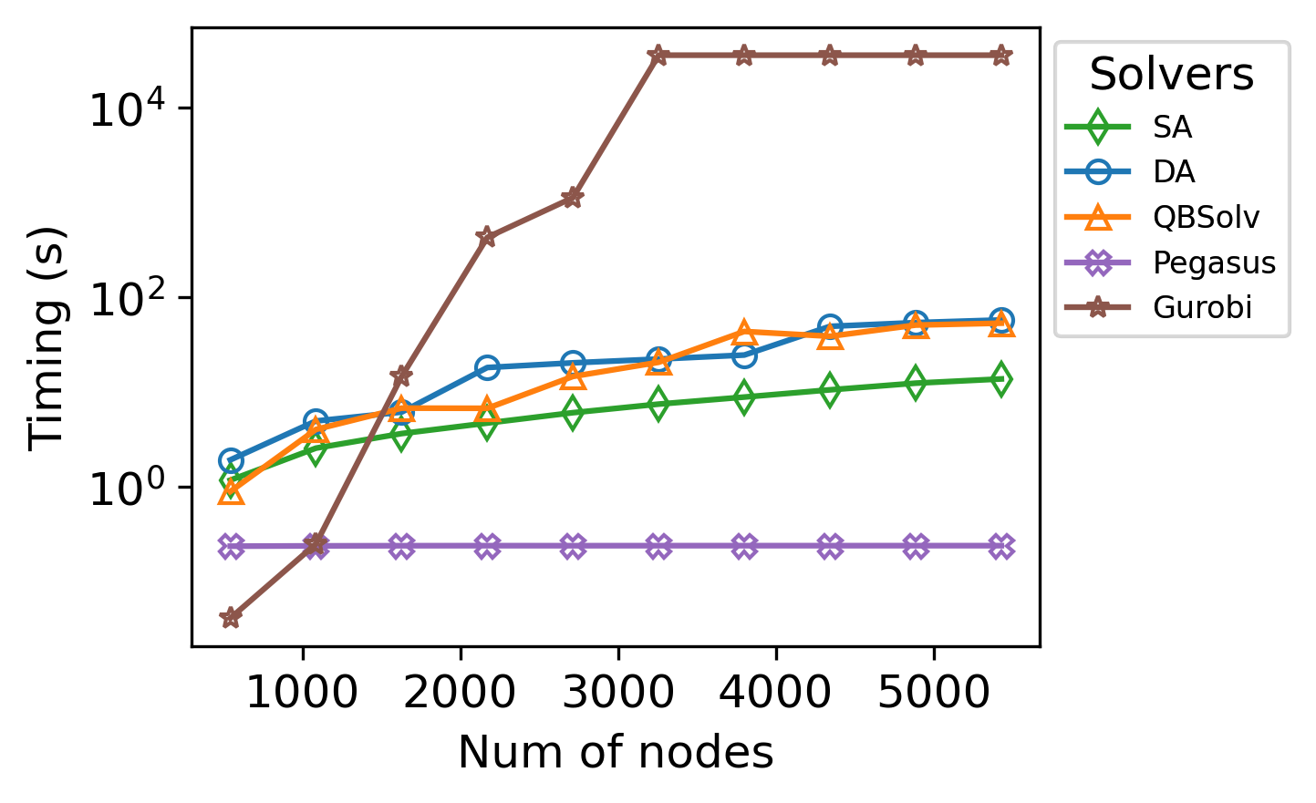
(a) Timing

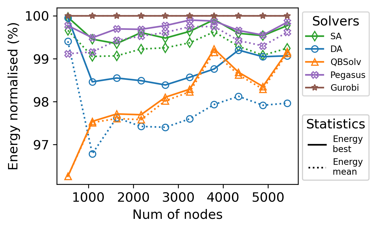
(b) Energy

Figure 1: Performance on Pegasus-like max-cut problems. X axis represents the number of nodes. (a) Timing. Y axis represents seconds in log scale. (b) Objective energy, normalised to that of Gurobi. Two statistics, mean energy (dotted lines) and best energy (solid lines), are included. For hyper-parameters, we use $T_{neal}=2000\mu s$ for D-Wave annealer, $\#iter=10^{6}$ for DA, and $\#sweep=10^{4}$ for SA

Fig. 1(a) shows the timing of the solvers on the Pegasus-like max-cut problems. Pegasus QPU spends about $200ms$ on all these problems. The total execution time of the QPU can be decomposed into programming time and sampling time. The sampling time is fixed because the QPU is based on the same annealing process. The programming time increases along with the problem size. Pegasus is generally 2-3 orders of magnitude faster then the classical annealing-based solvers. The difference in timing mostly comes from the fundamental difference in the working principles. The solving time of classical solvers depend on the size of a problem. Larger problem usually requires longer running time. The solving time of Gurobi increases sub-exponentially along with the size of the problem. Because we set the Gurobi program to terminate when its running exceeds ten hours, the second half of the Gurobi curve clips.

Fig.1(b) shows the objective energy, normalised to that of Gurobi. To describe the statistics of the results, we use solid curves to represent the energy of the best solution, and use the dotted curves to represent the mean energy of the solutions. Since max-cut is a maximisation problem, higher energy is better. The energy achieved by classical annealers and quantum annealer is not closely related with problem size. This experiment demonstrates the scalability of classical and quantum annealers. Pegasus outperforms all classical annealers on most of the problem instances by a margin of $1\%-3\%$ energy. DA performs better on the problem instances of size over 4000, which have higher connectivity than what smaller instances have.

We also have experiments on Chimera-like max-cut problems. Please find the details in the Appendix C.2.

3.1.2 Connectivity-varied max-cut problems

The Pegasus-like graph in the previous section is sparsely connected graphs and are not in favour of DA. According to Fujitsu’s official documentation Aramon et al. (2019), DA is designed for solving optimisation problems with densely connected graphs. In this section, we examine how connectivity affects the performance of an annealer. We make 32 randomly generated max-cut graphs, each of which has 145 nodes. The average degree of these graphs ranges from 1 to 140. For the Pegasus QPU, there will be auxiliary qubits and connections involved in the final embedding, since the connectivity-varying problems are mostly not a sub-graph of the Pegasus graph architecture.

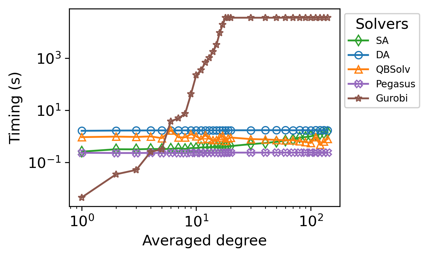
(a) Timing

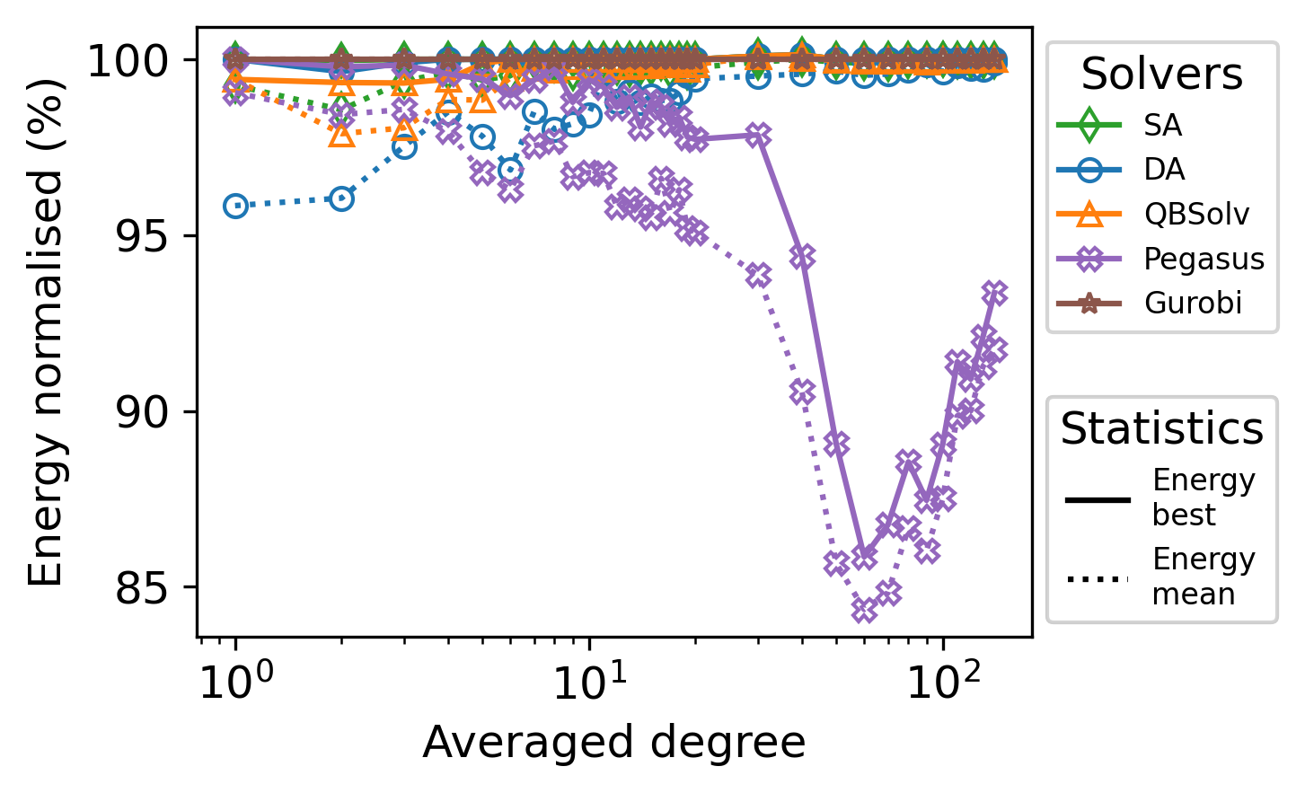
(b) Normalised energy

Figure 2: Performance on connectivity-varied max-cut problems. The plot setting is similar to that in Fig.1. For hyper-parameters, we use $T_{neal}=2000\mu s$ for D-Wave annealer, $\#iter=10^{6}$ for DA, and $\#sweep=10^{4}$ for SA

Fig.2(a) shows the time consumption of all solvers. Problems with degree over ten are challenging such that Gurobi cannot quickly traverse the solution spaces, so we set a timeout limit of ten hours. On the other hand, there are only 145 nodes in these graphs, which is “trivial” for classical annealers. DA, SA and QBSolv finish searching within one second, which is very close to the timing of Pegasus.

Fig.2(b) shows the objective energy of the solutions. All solvers, except Pegasus, can achieve 100% energy on almost all problem instances. The mean energy of DA improves as the connectivity increases. We have similar observations in Section 3.1.1, where the energy of DA improves as problem size increases. This suggest that DA performs better on densely connected problems. In comparison, the energy of Pegasus decreases when averaged degree is over 12. The mean energy could drop down to as low as 85%, which corresponds to averaged degree of 16. This suggests the Pegasus performs better on sparsely connected problems.

The problem setting of max-cut is straightforward. Many other problems have constraints that cannot be directly represented in existing annealers. An annealer may find a solution that violate the constraints. We shall see how the situation changes for such problem settings.

3.2 Minimum Vertex Cover

Given an undirected graph with a set of nodes $V$ and edges $E$, a vertex cover of a graph is a set of nodes that includes at least one endpoint of every edge of the graph. The Minimum Vertex Cover (MVC) problem is an optimisation problem that finds the smallest vertex cover of a given graph. MVC problem can be formulated as eq.2.

$$\mathrm{Minimize}\sum_{i\in V}x_{i}\quad\text{subject to}\quad x_{i}+x_{j}\geq 1,\;\forall(i,j)\in E$$ (2)

$x_{i}=1$ indicates node $i$ is in the cover and $x_{i}=0$ otherwise. The objective function minimises the number of nodes in the vertex cover, whereas the constraints ensure that at least one of the endpoints of each edge $(i,j)$ will be in the cover. In a quantum(-inspired) annealer, there is no corresponding mechanism to ensure the satisfaction of the constraints. A workaround is to lift the energy of configurations that violates the constraints and such that it becomes a less favourable solutions. This method is widely known as “penalty”. The penalty of MVC can be formulated in the form of $\alpha\cdot(1-x_{i}-x_{j}+x_{i}x_{j})$, where $\alpha$ represents a positive scalar penalty. A QUBO form for MVC is given by:

$$\mathrm{Minimize}\;\sum_{i\in V}x_{i}+\alpha\sum_{(i,j)\in E}(1-x_{i}-x_{j}+x_{i}x_{j})$$ (3)

The penalty term does not introduce new connections to the graph. The QUBO form has the same topology as that of the original problem. The choice of penalty weight $\alpha$ is application-specific. For eq.3, adding a node to a minimum vertex cover will increase the objective energy by one. Removing any node from a minimum vertex cover will increase the objective energy by $\alpha-1$. Glover et al. (2019) suggest any $\alpha>1$, for example, $\alpha=2$ would ensure that a solver can find solutions that satisfy the constraints of a MVC problem.

3.2.1 Connectivity-varied MVC problems

We reuse the connectivity-varied graphs in Section 3.1.2 for constructing MVC problems. We discover that some solvers have difficulty in finding feasible solutions with penalty weight $\alpha=2$. We set $\alpha=\max_{i\in V}\deg(i)$, which represents the highest degree in a graph. With this setting, we can understand the comparison between the annealers more clearly.

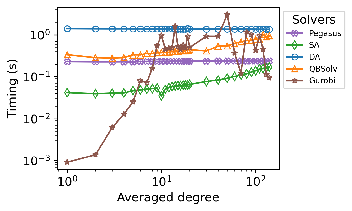
(a) Timing

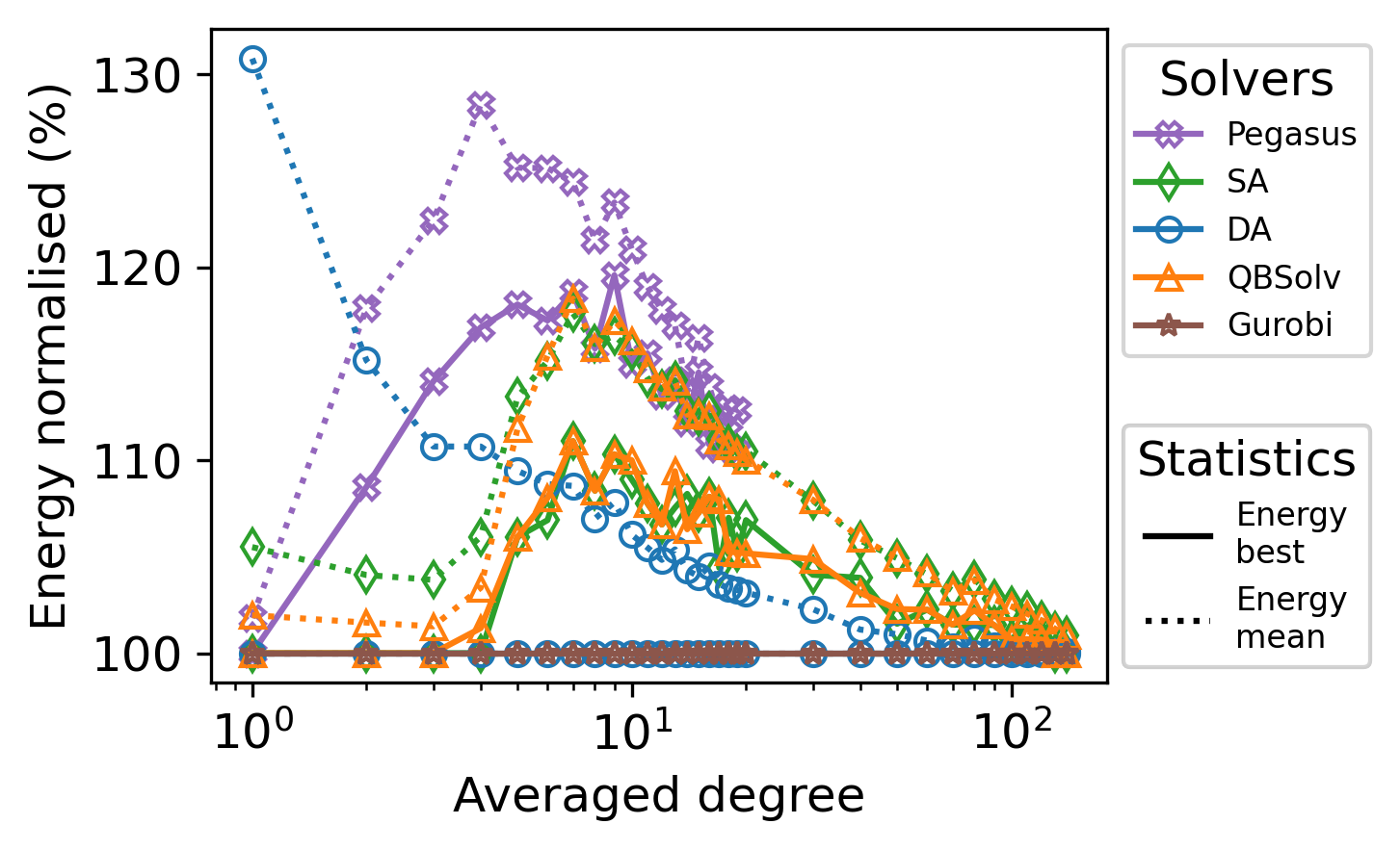
(b) Normalised energy

Figure 3: Performance on connectivity-varied MVC problems. The plot setting is similar to that in Fig.1, except that infeasible solutions are not counted in Fig.3(b). For hyper-parameters, we use $T_{neal}=2000\mu s$ for D-Wave annealer, $\#iter=10^{5}$ for DA, and $\#sweep=10^{2}$ for SA

Fig.3(a) shows the timing of the solver on the connectivity-varied MVC problems. Since we are using $T_{neal}=2000\mu s$ for Pegasus, it loses its leading position in terms of timing. This figure is similar to Fig.2(a), except the timing of Gurobi stops increasing when the averaged degree is above 10. All solutions obtained by Gurobi are global optimal solutions.

Fig.3(b) shows the objective energy of solutions, normalised to that of Gurobi. Since MVC is a minimisation problem, lower energy is better. The best energy curve of DA is always at 100%, which means it finds optimal solutions for all problems. It is overlapped with Gurobi. One can spot the markers of DA and Gurobi by zooming in. Pegasus find the optimal solution only when the average degree is equal to one. Then there is more than 20% performance drop as the degree increases. The Pegasus curve does not continue beyond a degree of 11 as it fails to find any feasible solution.

In annealing-based methods, we sample multiple times for a problem instance. If a problem has constraints, some samples of the QUBO form may not be feasible, i.e., does not satisfy with constraints. We introduce a metric called probability of feasibility, or $P_{f}$:

$$P_{f}=\frac{\text{Feasible \#samples}}{\text{Total \#samples}}\times 100\%$$ (4)

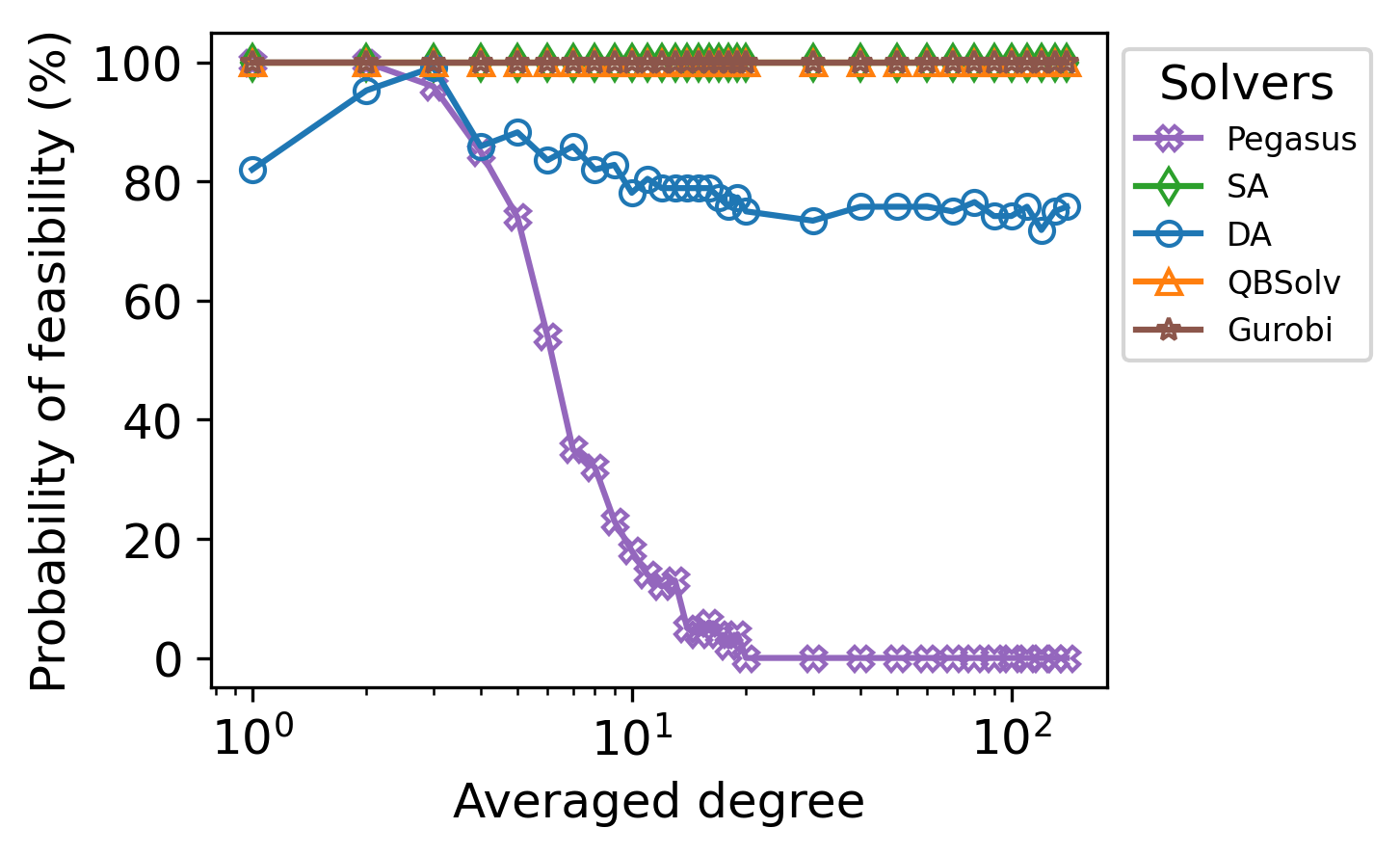
(a) Probability of feasibility

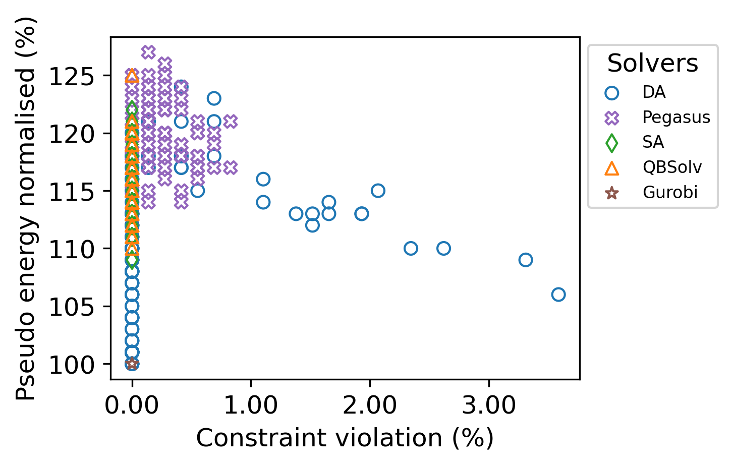
(b) Constraint violation

Figure 4: Feasibility in connectivity-varied MVC problems. a) X axis is averaged degree in log scale. Y axis is $P_{f}$ in percentage. Gurobi, SA and QBSolv always achieve 100% $P_{f}$, the curves of which are overlapped with each other and cannot be seen, but one can spot their markers by zooming in. b) The distribution of constraint violation on the problem instance with an averaged degree of 10. X axis is the constraint violation in percentage. Y axis is pseudo objective energy, normalised to that of Gurobi.

Fig.4(a) shows the relation between averaged degree and $P_{f}$. The SA curve is always 100%, which provides a sanity check of the choice of the penalty coefficient $\alpha$. The Pegasus curve drops to zero when the degree goes beyond 11. This is where the Pegasus curve stops in Fig.3(b). The Pegasus curve suggests it is struggling to find feasible solutions as the average degree increases. In fact, for the problem with 140 degrees, we have fine-tuned $\alpha$, or even remove the objective and solve the constraints solely, and still cannot find any feasible solution. DA in Fig.4(a) achieves about 80% $P_{f}$. With higher $\#iter$, e.g. $10^{6}$, it achieves 100% all the time. Gurobi always find feasible solutions because the constraints can be explicitly implemented in Gurobi and directly regulate the searching process.

We further investigate the constraint violation in a solution. This is for us to understand how easy it is to fix the violation and salvage promising solutions from broken ones. For MVC, the number of constraints is equal to the number of edges in a graph, according to eq.2. If two decision variables on two sides of an edge are all zeros, we count it a violation. We divide the number of violations in a solution by the number of constraints, and name the result as the percentage of constraint violation. We use pseudo energy to measure the quality of infeasible solutions, which is the original objective energy plus the non-zero penalty terms.

We examine the problem of degree equals to 10, because this is one of the most challenging instances, according to the time consumption of Gurobi. The relation between energy and constraint violation is shown in Fig.4(b). Each marker represents a solution. The left bottom corner, i.e., the coordinate (0.0, 1.0), is the global optima. The solutions of QBSolv and SA reside on the line of violation=0.0%, which means these solutions are feasible. On the other hand, many solutions from Pegasus distribute across 0%-1%, which are infeasible solutions. The distribution of the infeasible solutions of DA is similar to a Pareto frontier, in which if you emphasize more on fewer violations, you get higher energy. In some cases, one can see a similar frontier in quantum annealer’s constraint violations, which is available in Appendix D and E. Fixing broken constraints is another broad topic, which falls out side the scope of this paper. If fixation is not an option, one can also use these infeasible solutions as initialisation of another search.

3.2.2 DIMACS 10th Challenge

We further evaluate the annealers on real and random datasets extracted from the 10th DIMACS Challenge Bader et al. (2013). Eleven graphs are included in this benchmark. The number of nodes ranges from 34 to 22963. Please find the detailed of dataset in Appendix D.3.

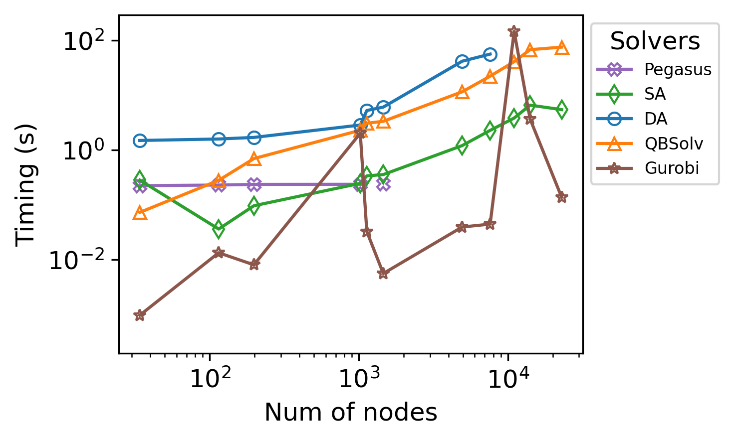
(a) Timing

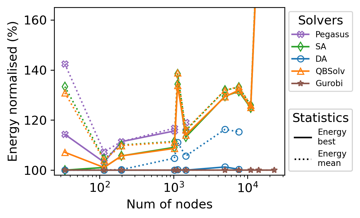
(b) Normalised energy

Figure 5: Performance on MVC problems from DIMACS 10th Challenge. The plot setting is similar to that in Fig.3. For hyper-parameters, we use $T_{neal}=2000\mu s$ for D-Wave annealer, $\#iter=10^{6}$ for DA, and $\#sweep=10^{2}$ for SA

In Fig.5(a), the timing of the solvers remains a similar trend compared to previous experiments. The Pegasus curve stops when the size of the problem is over 1024 because D-Wave’s minor embedding heuristic failed to map larger problems onto Pegasus. DA cannot handle the problem size over 8192.

According to Fig.5(b), DA outperforms Pegasus in terms of the quality of solutions, as well as problem size. If we check with Fig.6(a), we know that Pegasus is struggling to find feasible solutions, when the problem size is over 100. This matches with the results in previous section. In comparison, the solutions found by DA are mostly feasible.

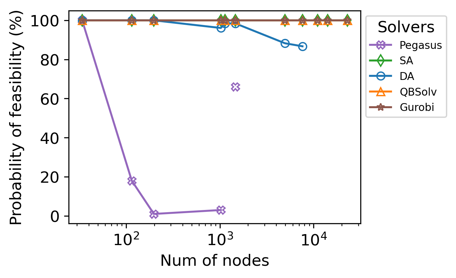
(a) Probability of feasibility

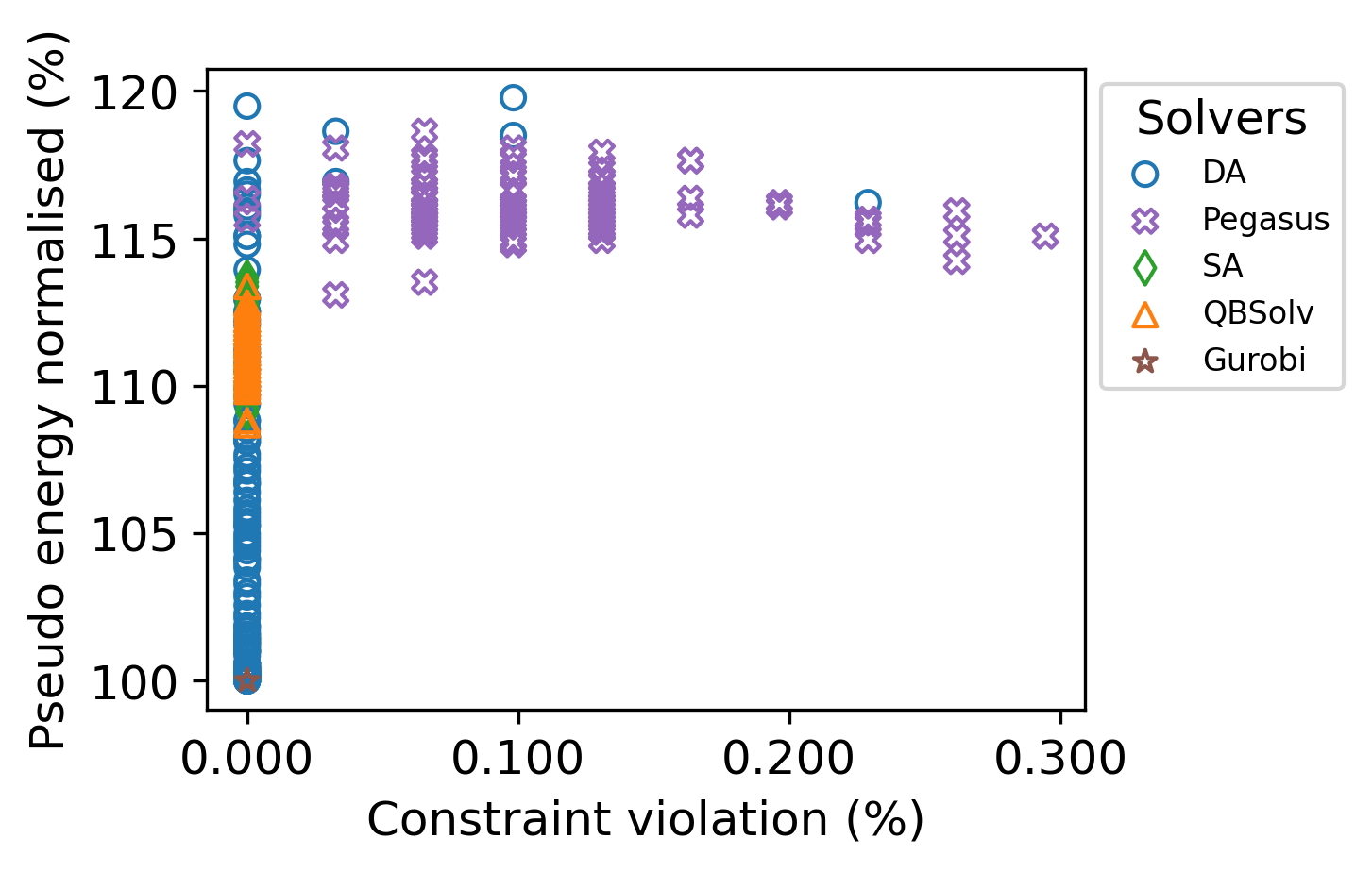
(b) Constraint violation

Figure 6: Feasibility on MVC problems from DIMACS 10th Challenge. The plot setting is similar to that in Fig.4. b) The constraint violation on the “delaunay_n10” problem

Fig.6(b) shows the relation between normalised energy and constraint violation on the famous “delaunay_n10” problem. We choose it because this is the largest that Pegasus can handle in this dataset. Most of the solvers have similar distributions of solutions, compared with Fig.4(b). For Pegasus, the distribution is not similar to a Pareto frontier. The normalised energy for Pegasus is around 1.18 and is independent of the constraint violation. We see this as a sign that the noises and errors overwhelm in the quantum annealer, such that the solutions are no longer related to the original problem.

We use the benchmark from DIMACS 10th Challenge in 2012, because we believe it closely follows the trend of requirements nowadays. However, most of the previous works on heuristic MVC methods are based on the benchmark from DIMACS 2nd Challenge in 1992. We evaluate benchmark from DIMACS 2nd as well and include the results in Appendix D.4. We also have experiments on a set of Pegasus-like MVC problems in Appendix D.1.

3.3 Quadratic Assignment Problem (QAP)

The Quadratic Assignment Problem (QAP) is a well-known combinatorial optimisation problem with a wide range of applications, such as backboard wiring, statistical analysis, placement of electronic components, etc.

QAP can be visualised as the problem of assigning $n$ facilities to $n$ locations. Between any two facilities, there are products transported back and forth, and the amount transported is called the flow. Between two locations there is some distance. Traffic is defined as the product of flow and distance. The problem is to assign facilities to locations such that the sum of traffic is minimised. The aim is to find an assignment of the facilities to the locations such that the sum of all products of flows and their corresponding distances is minimised, subject to the constraints that each facility is assigned to exactly one location and each location contains exactly one facility.

Formally, we assume $n$ is the number of facilities which is also the number of locations. $F=(f_{ij})$ is the flow matrix for facilities. Each entry represents the flow between facilities $i$ and $j$. $D=(d_{kl})$ is the distance matrix. Each entry represents the distance between location $i$ and $j$. $X=(x_{ij})$ is the binary decision matrix. Each entry represents whether facility $i$ is assigned to location $j$. Note that the dimension of $X$ is $n\times n$, which implies that there are $O(n^{2})$ binary decision variables. If the flow is given as the matrix $(f_{ij})$ and distance is given as the matrix $(d_{kl})$, then the objective function to minimise is:

Minimise $$\sum_{i=1}^{n}\sum_{j=1}^{n}\sum_{k=1}^{n}\sum_{l=1}^{n}f_{ij}d_{kl}x_{ik}x_{jl}$$ (5)

subject to $$\sum_{k=1}^{n}x_{ik}=1\qquad\forall 1\leq i\leq n$$ (6)

and $$\sum_{i=1}^{n}x_{ik}=1\qquad\forall 1\leq k\leq n$$ (7)

$x_{ik}$ is the binary decision variable representing whether facility $i$ goes to location $k$. The constraints ensure that one facility is assigned to a location exactly once.

To enable the annealing of a QAP, we have to subsume constraints eq.6 and 7 as a part of the objective function eq.5. Conventionally, we can encode the constraints as penalty terms which augment the objective function.

$$\begin{split}\text{Minimise}\quad&\sum_{i=1}^{n}\sum_{j=1}^{n}\sum_{k=1}^{n}\sum_{l=1}^{n}f_{ij}d_{kl}x_{ik}x_{jl}\\ +&\alpha(\sum_{k=1}^{n}x_{ik}-1)^{2}+\alpha(\sum_{i=1}^{n}x_{ik}-1)^{2}\end{split}$$ (8)

Eq.8 is a standard QUBO form of QAP. $\alpha$ is a penalty weight, which connects the original objective function eq.5 and the constraints eq.6 and 7. It can be shown that for QUBOs, the optimal solution to the augmented objective function also minimises the original objective function.

3.3.1 TinyQAP

A QAP with $n$ facilities and $n$ locations have $n^{2}$ variables, which often yields large models in practical settings. Compared to the max-cut and MVC problems, QAP is more demanding on the number of qubits. All problems in QAPLIB Burkard et al. (1997) are beyond the capability of a quantum annealer.

We generate a set of tiny QAP problems to facilitate the evaluation of quantum annealers. The problem size ranges from 3 to 12. We set penalty weight $\alpha=n\times\mathrm{max}\left(\left|C\right|\right)$, where $C$ represents a list of the coefficients of all linear and quadratic terms in eq.5. This setting follows the suggestion in Glover et al. (2019) about the “Scalar Penalty $P$”, with a little more emphasis on the feasibility. The settings are applied to all experiments in Section 3.3.

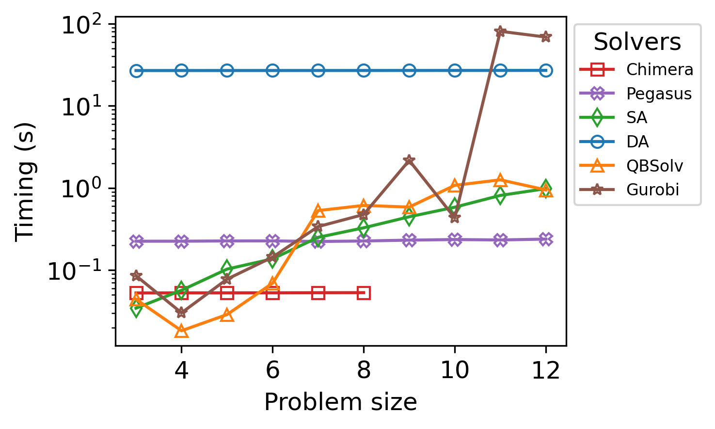
(a) Timing

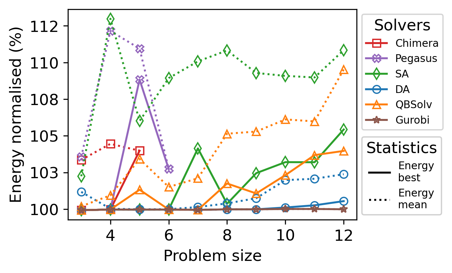
(b) Normalised energy

Figure 7: Performance on TinyQAP. The plot setting is similar to that in Fig.3. For hyper-parameters, we use $T_{neal}=200\mu s$ for D-Wave Chimera, $T_{neal}=2000\mu s$ for D-Wave Pegasus, $\#iter=10^{8}$ for DA, and $\#sweep=10^{3}$ for SA

In Fig.7(a), Chimera and Pegasus are not the fastest. The Chimera curve stops at 8, which corresponds to 64 decision variables. The largest complete graph that Chimera accepts is 65. QAP of $n=12$ is the up-limit of a Pegasus QPU can handle. DA is not designed for such trivial optimisation problems. We can see that the timing of DA does not scales up as the problem size increases.

As shown in Fig.7(b), Chimera only finds feasible solutions when $n\leq 4$. From Fig.8(a) We know that the $P_{f}$ of Chimera quickly drops to 0% when $n>4$. The Pegasus QPU managed to find feasible solutions for $n=5$, but its $P_{f}$ is very close to that of Chimera. This suggests Pegasus architecture does not have a clear advantage over the Chimera architecture. Please note that we are using quite large $T_{anneal}$ for Chimera and Pegasus, which generally leads to better feasibility. For Chimera, increasing $T_{anneal}$ by a factor of 10 does not give any improvement in terms of $P_{f}$, so we just demonstrate the results of $T_{neal}=200\mu s$. DA can find very promising solutions, which are all feasible and very close to the global optima.

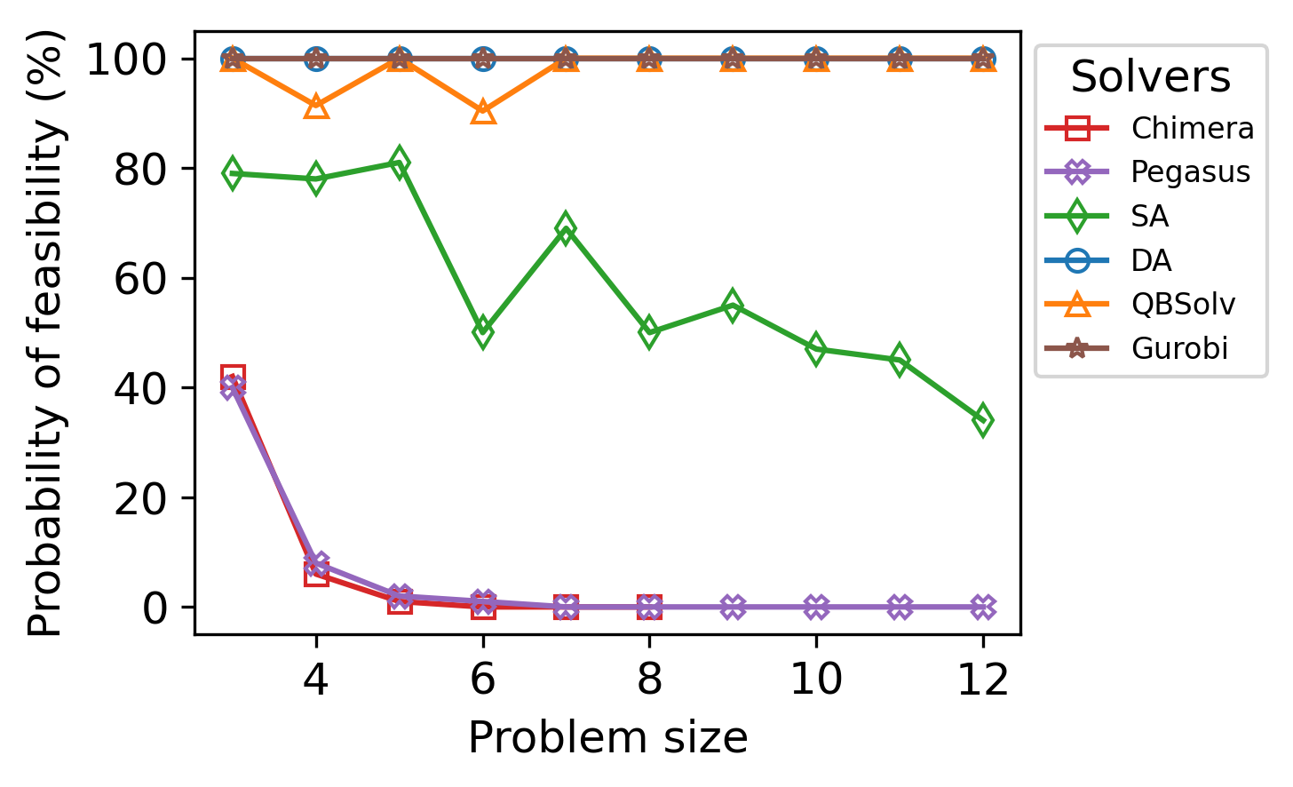
(a) Probability of feasibility

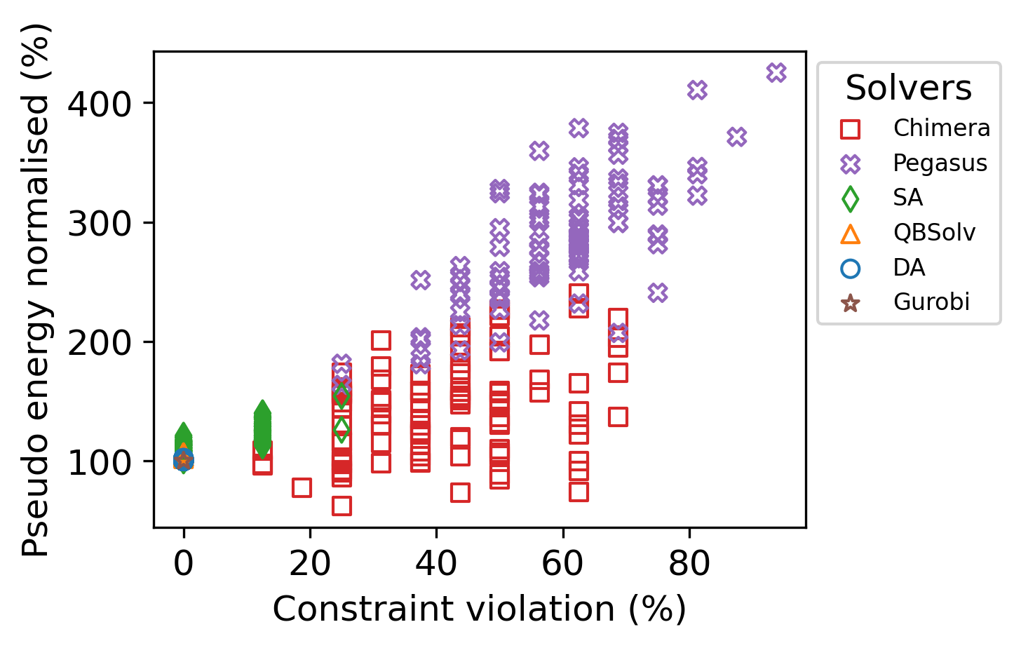
(b) Constraint violation

Figure 8: Feasibility on TinyQAP. The plot setting is similar to that in Fig.4 b) The constraint violation distribution on “tiny-08”.

We also investigate the constraint violation of the solutions to “tiny-08”, which allows us to compare Chimera and Pegasus. The constraints in QAP are one-to-one mapping constraints. For example, in the tiny-03 problem, we have 6 constraints, i.e., 3 constraints to ensure each facility is only assigned to one location, and another 3 constraints to ensure each location only accommodates one facility. From Fig.8(b) we see the solutions of QBSolv and DA reside at coordinate (0.0, 1.0), which means these solutions are all feasible and optimal. Some of the solutions of SA are infeasible, but with only one or two violations.

In comparison, the two quantum annealers are suffering from many constraint violations. From Fig.8(b) we see the energy distribution of Chimera and Pegasus is roughly proportional to the number of violations. This is partly because we put more emphasis on the feasibility of a solution and put high penalty in the objective energy. With the same penalty settings, the annealing-based classical solvers find feasible and competitive solutions most times, but neither of the two quantum annealers can find any feasible solutions. In fact, we have fine-tuned $\alpha$. We even try to solve the penalty term solely. Neither of the quantum annealers find any feasible solutions. We believe this is partly due to the mis-implementation of the problems on the quantum annealers because of the analog control errors in QPUs. Pearson et al. (2019). In this experiment the solutions of Chimera is closer to the optimal solution compared with Pegasus. However we cannot assert Chimera architecture is better than Pegasus, because we only have access to one QPU instance of each architecture and cannot rule out the impact of individual differences in the performance evaluation.

TinyQAP is too small for DA. We are going to push towards the limit of DA in the next experiment.

3.3.2 QAPLIB

We choose the Tai dataset from QAPLIB Burkard et al. (1997) because the size fits well with the purpose of our evaluation. We only use the instances Taixxa, which are uniformly generated. We do not include quantum annealers in this experiment because most of the problems are too large for them.

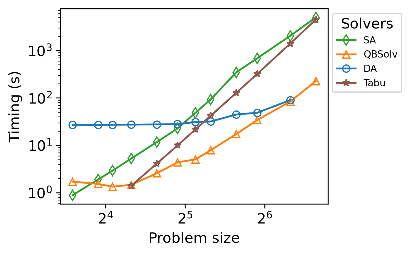
(a) Timing

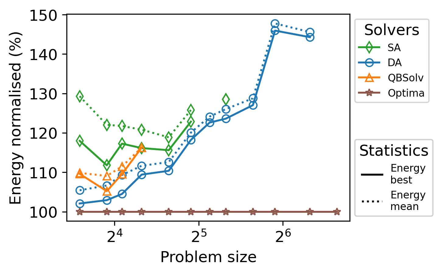
(b) Normalised energy

Figure 9: Performance on Tai benchmark. The plot setting is similar to that in Fig.3. For hyper-parameters, we use $T_{neal}=2000\mu s$ for D-Wave Pegasus, $\#iter=10^{8}$ for DA, and $\#sweep=3\times 10^{3}$ for SA. We obtain global optima from Burkard et al. (1997). The timing of Tabu algorithm is from Misevicius (2005)

According to Fig.9(a) DA has its advantage over SA when the problem size is over 30. It also outperforms SA and QBSolv in terms of objective energy in Fig.9(b). The hybrid method QBSolv find better solutions than SA, but not as good as DA. We also observe that both SA and QBSolv have difficulty in finding feasible solutions, according to Fig.10(a)

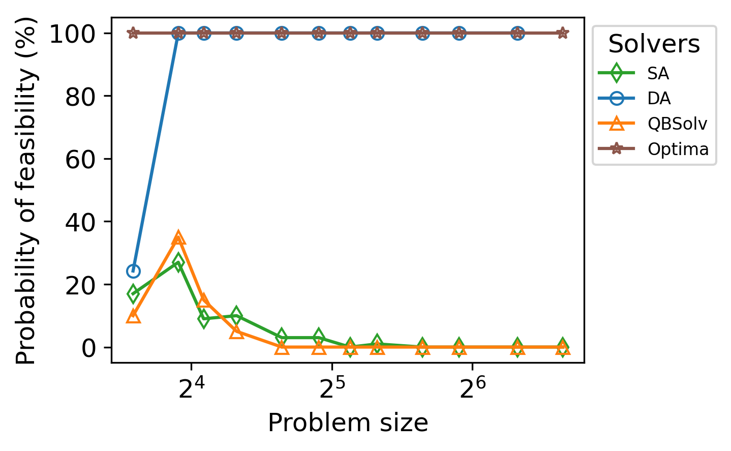
(a) Probability of feasibility

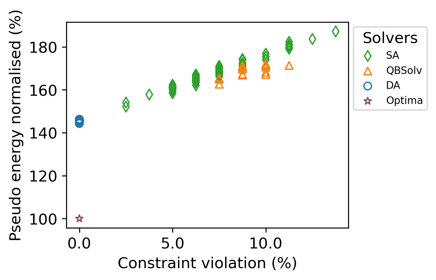
(b) Constraint Violation

Figure 10: Feasibility on Tai benchmark from QAPLIB. The plot setting is similar to that in Fig.4 b) The constraint violation distribution on “tai80a”.

Fig.10(b) is the constraint violation of solutions to “tai80a”. We choose this problem because it is the largest one in the dataset that can be handled by DA. All solutions of DA feasible. For SA and QBSolv, although none of their solutions is feasible, there is only about 3-15% of constraint violation, which means the violation fixation task is not very challenging.

Warehouse management is a representative application of QAP. A warehouse usually has items and locations that are much larger than the problem size in previous QAP datasets. We aim to develop a scalable method and facilitate Warehouse management problems with the power of quantum(-inspired) computers.

4 The Warehouse Assignment Problem

In warehouse management, order picking is a labour-intensive and costly activity. Tsige (2013) Consider the problem of assigning items to locations in a warehouse. How should the storage assignment be done, so that when orders come in and items are picked, the travel distance of the picker is at a minimum? For a company, the reduction of such distance translates to the reduction of labour costs. The objective is to find a decent assignment that minimises the travel distance for a given set of orders.

Consider a warehouse with a layout of Fig.11(a). It has three aisles and 30 locations in total. Each aisle can reach the two columns on its left and right. There is an Input/Output (I/O) point at the bottom left corner through which items are transported in and out of the warehouse.

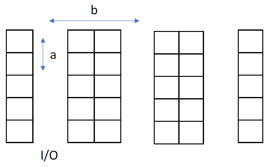
(a) Warehouse layout example

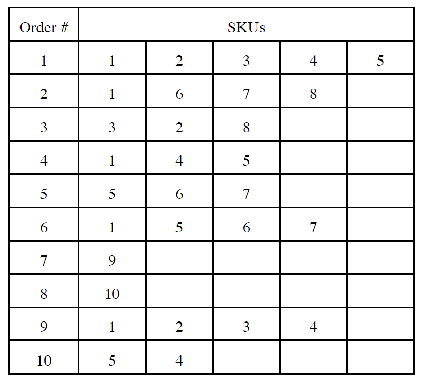
(b) Example of a set of orders

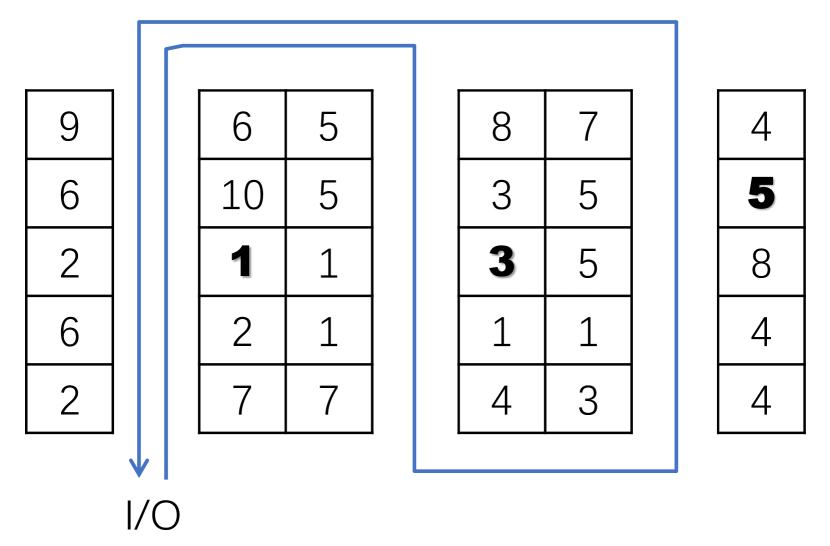
(c) S-shaped routing policy

Figure 11: Warehouse Assignment Problem

A set of orders is shown in Fig.11(b). There are 10 orders and 10 storage keep units (SKUs). An SKU represents a unique type of item. The 10 SKUs are labelled 1 to 10. There are a total of 30 items, each of which belongs to a particular SKU.

To pick an order, the picker always starts from the I/O point. It may follow a different route to collect all items. Among various routing strategies, S-shaped (traversal) is the most common and simplest routing policy used in practice. Tsige (2013) With this policy, the order picker begins by entering the aisle closest to the I/O point. If an aisle contains at least one item, the picker traverses the aisle over the entire length, otherwise, the picker skips that aisle. After picking the last item, the order picker takes the shortest route back to the I/O point. In this paper, we applied a modified S-shaped routing policy, in which a picker will not skip an aisle if there is no item in it. The modification provides a better match between the objective function of the warehouse assignment problem and QAP. An example of the S-shaped routing policy is illustrated in Fig.11(c). The picker collects the highlighted item in the first and last aisle by following an S-shaped route even if there is no item to pick in the second aisle.

It is easy to apply QAP to the setting of warehouse assignments. Ruijter (2007) To do so, simply replace “facilities” with “items”. The flow between items is defined to be the frequency at which their respective SKUs appear in the same order. This can be computed based on the incoming order set. The distance between locations is routing-specific. With our revised S-shaped routing policy, the distance between two items is roughly proportional to the number of columns between them, since the picker would in principle traverse those columns in a zig-zag manner.

4.1 Heuristics: Block Structure

What inspires the application of QAP in warehouse assignment is the idea to assign items with high flow closer to each other. Intuitively, this would reduce the amount of traffic in picking orders because the picker is more likely to travel a shorter distance in between items appearing in the order.

The block structure of QAP occurs in the distance matrix $(d_{ij})$. Suppose $V(H)$ is the nodes in a graph of the locations. There is a partition of $V(H)$ into $K$ subsets and a function that maps each location to its respective subset: $c:V(H)\rightarrow K$, where $K={1,2,\ldots,k}$, such that

$$d(x,y)=\begin{cases}\delta(x,y)&\text{ if }c(x)=c(y)\\ M(x,y)&\text{ if }c(x)\neq c(y)\end{cases}$$ (9)

where $\delta$ and $M$ are both functions. The concrete functions would depend on $d$, but with block structure $\delta$ would “usually” return smaller values than $M$. A special case is when $\delta$ and $M$ are constant with $\delta<M$, and $(d_{ij})$ will be a “block matrix”.

Consider an example with the following warehouse of 8 locations, with each location labelled as in Fig.12(a). Assume that the vertical distance is 1 and the horizontal distance is 3. The distance matrix looks like the one in Fig.12(b) (only the upper triangular part is shown).

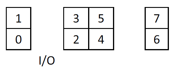
(a) Toy layout

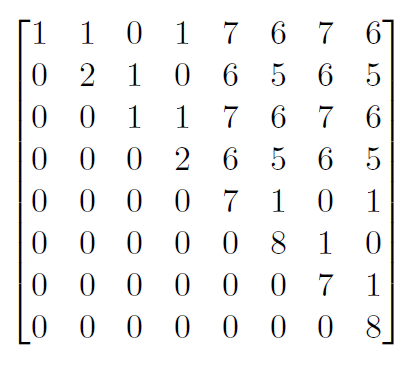
(b) Toy layout distance matrix

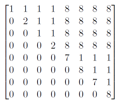
(c) Simplified distance matrix

Figure 12: Demonstration of block structure

Noticeably, the $4\times 4$ sub-matrix in the upper right corner, corresponding to the distance between the 1st and the 2nd aisles, is uniformly larger in number than the sub-matrices near the diagonal. In general, we could relabel the indices of locations such that the columns of a warehouse form intervals, and that when we move away from the diagonal, the matrix entries become larger because the columns are further away.

Since the above block-structure is observed, one simplification is that all locations within the same column have distance 1 (i.e. $\delta\equiv 1$) in between, and all locations in different columns have a larger distance, say 8 (i.e. $M\equiv 8$). Then the block structure becomes more pronounced as shown in Fig.12(c). Please note that the diagonal of the distance matrix represents the distance between the entry and a certain location. The calculation of the diagonal does not follow the block structure. That’s why the diagonal is the same in Fig.12(b) and Fig.12(c).

The simplification would normally be expected to flatten the energy landscape and remove tall and thick energy barriers. This benefits annealing-based computers, since energy barriers are notoriously challenging to both quantum and classical annealers. Quantum annealers use quantum mechanics to overcome energy barriers. For classical annealing, the parallel tempering method in DA and many other methods are proposed to overcome energy barriers. A flattened energy landscape is generally easier for annealing-based solvers to work with.

Similar to the way we can perform partitioning on locations, the item set can also be partitioned into $K$ of equal size, where $K$ is fixed to be $|K|$. Intuitively, we want items to appear together in high frequency to be assigned closer to each other. Therefore, we maximise the sum of interaction frequencies within the subsets and then assign each subset to a subset in the partition of $V(H)$, the set of locations. Note that $K$ divides $n$ is assumed, so that locations and items can be divided evenly.

4.2 Decomposition

Next, we describe the decomposition formally and provide proof of the theoretical boundary. To minimise the travelling distance, intuitively, we want to maximise the interaction frequencies of items within a block. This objective can be formally described as follows:

$$\text{Maximise}\quad\sum_{i,j=1}^{n}\sum_{l=1}^{k}f_{ij}x_{il}x_{jl}$$ (10)

Eq.10 denotes the sum of interaction frequencies among items within their respective subsets. $(x_{ij})$ is an $n\times k$ decision matrix. $x_{ij}$ denotes whether item $i$ goes to subset $j$. The objective comes with the following constraints:

$$\sum_{l=1}^{k}x_{il}=1\quad\forall i,1\leq i\leq n$$ (11)

$$\sum_{i=1}^{n}x_{il}\leq s\quad\forall l,1\leq l\leq k$$ (12)

Eq.11 means an item belongs to exactly one subset. Note that each subset can have at most $s=\frac{n}{k}$ items. Therefore, eq.12 means each subset must not exceed its capacity $s$.

Note that eq.10 is actually another QAP with a particular decision matrix (but with different constraints). Thus, it can be translated into a graph formulation. Suppose $V(G)$ and $E(G)$ are the nodes and edges in a graph of items. In the graph formulation, $(x_{ij})$ is equivalent to a function $g:V(G)\to K$, which maps an element of $V(G)$ into its subset, such that $g(i)=a\iff x_{ia}=1$. This function is well-defined due to constraint eq.11. Eq.10 can be converted to the equivalent graph formulation as follows:

$$\sum_{i,j=1}^{n}\sum_{l=1}^{k}f_{ij}x_{il}x_{jl}=\sum_{\begin{subarray}{c}(i,j)\in E(G)\\ g(i)=g(j)\end{subarray}}f(i,j)$$ (13)

which, intuitively, is the sum of flows within subsets. This is the setup for the theorem below, which states that with a solution to eq.10, an optimal solution to the overall QAP eq.5 can be constructed. The proof is available from Appendix F.5.

Theorem 1.

Let $d(x,y)=\begin{cases}\delta&c(x)=c(y)\\ M&c(x)\neq c(y)\end{cases}$ for some positive constants $\delta$ and $M$. Then there exists a $\varphi_{0}$ for which eq.5 is achieved, and $\varphi_{0}$ can be constructed from a solution to eq.10 denoted by $g_{0}$.

This theorem assumes a strong condition that $(d_{ij})$ only has two distinct values, $\delta$ for locations within an interval and $M$ in between intervals. This is a simplification of the block structure and $(d_{ij})$, in reality, is usually more complex.

However, the concept of intervals can be generalised such that when $\delta$ and $M$ are non-constant, a function $c$ can still be defined on $V(H)$ such that the sum of distances within intervals is minimised. The motivation for such construct is that when a warehouse does not exhibit a clear-cut column structure, one can still think of an abstract “column” as a group of close locations. Note that this definition automatically specialises to the previous definition of $c$ when $\delta$ and $M$ are constant. This intuition can be formally expressed as

Minimise $$\sum_{i,j=1}^{n}\sum_{l=1}^{k}d_{ij}x_{il}x_{jl}$$ (14)

Subject to $$\sum_{l=1}^{k}x_{il}=1\quad i\in[1,n]$$ (15)

and $$\sum_{i=1}^{n}x_{il}\leq s\quad l\in[1,k]$$ (16)

$(x_{ij})$ is an $n\times k$ decision matrix. $x_{ij}$ denotes whether item $i$ goes to location group $j$. Note that this graph partitioning problem can be thought of as the dual to eq.10, with maximisation changed to minimisation. In effect, items that are frequently ordered together will be assigned to locations that are closer together.

Now both the set of locations and the set of items have been divided into subsets of equal size. Between subsets of locations, the distances are maximal, and between subsets of items, the interaction frequency is minimal. The final step is to produce a bijection from the set of subsets of items to the set of subsets of locations, and for each pair of subsets in the bijection $(items,locs)$, there is a sub-QAP of size $O(\sqrt{n})$, and therefore a QUBO of size $O(n)$, where $n$ is the total number of items.

Note that this is subject to $n$ being a perfect square; in practical situations where $n$ is not a perfect square, compromise has to be made in either finding the nearest smaller perfect square and do the optimisation on the smaller set of items and locations only, or use integer divisors of $n$ other than $\sqrt{n}$, and correspondingly deal with sub-QAPs of sizes other than $\sqrt{n}$. For example, if there are $n=3600$ locations, it is possible to divide it into 40 groups of 90, where each sub-QAP will have $n=90$.

The overall procedure runs the decomposition in Subsection 4.2 and then solves each individual sub-QAP using the exterior penalty method. Each sub-QAP utilises a conversion procedure to transform it into QUBO solvable by quantum (-inspired) annealer. Finally, the procedure forms global solutions by aggregating solutions to sub-problems. The details of the overall procedure, the exterior penalty method and the conversion procedure are available in Appendix F.6 and F.7.

5 Experiments

The experiment has three objectives, namely 1) to evaluate the performance of the QAP decomposition heuristic in solving block-structural QAPs of various sizes, 2) to evaluate the effectiveness of the heuristic in minimising the warehouse picking distance, and 3) compare the performance of various computing hardware using different decomposition heuristics. In addition, we also included the heuristic algorithm “Tabu search” as a reference.

5.1 Comparison on QAP

We compare the performance of decomposition on QAP. Block-structural QAP instances WH-8, WH-90, WH-180, WH-270, WH-3600, and WH-8100 are synthesised using randomly generated order sets. The number corresponds to the size of a problem. The results obtained for each of the datasets are average values over three runs. Please refer to Appendix F.3 for details of dataset and experimental settings.

Table 1: QAP time comparison

Size	8	90	180	270	3600	8100
$T_{\text{QA}}$	0.016	-	-	-	-	-
$T_{\text{QBSolv}}$	0.37	379.95	7454	-	-	-
$T_{\text{DA}}$	3.70	23	-	-	-	-
$T_{\text{decomp}}$	-	-	60	68	983	2080
$T_{\text{Tabu}}$	0.02	0.08	0.15	0.19	23.5	64.3
$T_{\text{SA}}$	683	556	716	594	3447	6884

QA can only handle QAP of size 8 due to the limitations in the D-Wave Chimera architecture. From Table 1 we know that QA is the fastest among all others. Table 2 shows the energy of the solution found by QA is the highest. This matches with the results of experiments in Section 3.3.

DA can directly handle up to QAP of size 90. $T_{\text{DA}}$ 16 times faster than QBSolv on WH-90. In terms of the quality of the solutions, DA finds near-optimal solutions to WH-8. Although DA can handle a problem size of 90 directly without decomposition heuristics, the $E_{\text{DA}}$ is distinctly higher than that of Tabu and SA.

For problems larger than 90, we use decomposition heuristics to tackle the problem. $T_{\text{decomp}}$ in Table 1 is the time for DA solving all sub-problems. It scales linearly with the size of the problem. In terms of the quality of the solution, our decomposition heuristic can find a solution that is 14.3% lower than that of the random solutions on WH-180. However, as the number of partitions increases, the optimality against the random solution vanishes. For example, on WH-8100, there is no difference in energy between random solution and the decomposition heuristic.

Table 2: QAP energy comparison (lower is better)

Size	8	90	180	270	3600	8100
$E_{\text{QA}}$	119	-	-	-	-	-
$E_{\text{QBSolv}}$	81	$0.71m$	NA	-	-	-
$E_{\text{DA}}$	81	$0.67m$	-	-	-	-
$E_{\text{decomp}}$	-	-	$2.21m$	$15.9m$	$12.9b$	$115b$
$E_{\text{Tabu}}$	80	$0.64m$	$1.95m$	$14.4m$	$10.9b$	$103b$
$E_{\text{SA}}$	81	$0.64m$	$1.96m$	$14.4m$	$10.6b$	$91.7b$
$E_{\text{Random}}$	-	$0.75m$	$2.58m$	$17.5m$	$13.1b$	$115b$

• ‘$m$’ stands for ‘$\times 10^{6}$’ while ‘$b$’ means ‘$\times 10^{9}$’.

Tabu is faster than all other methods on most datasets, except WH-8. In terms of the solution’s quality, both Tabu and SA can find better solutions than other methods. QBSolv did not find any feasible solution for WH-180.

5.2 Comparison on Warehouse Management

We also generate a set of warehouse problems to test the effectiveness of the decomposition heuristic in reducing warehouse travel distance. The input data distribution is perturbed to provide modified versions of datasets in Section 5.1. The name of the resulting problems has a tailing letter “b”. This is to match the findings in Tsige (2013) that interaction-based methods such as QAP work well when 80% of ordered items are concentrated in 20% of the SKUs. In other words, there is a small set of commonly ordered products. The above assumptions are made about the order sets as well as the shape of the respective warehouses.

Table 3: Warehouse travel distance comparison

Name	ABC	COI	OOS	Random	decomp
WH-90b	733	876	773	741	765
WH-180b	1418	1434	1425	1418	1422
WH-270b	3457	4524	3084	3619	3098

A simulation framework is built to calculate the distance travelled given order, and an assignment. We include three representative assignment heuristics, i.e., Cube-per-order Index (COI) Malmborg and Bhaskaran (1990), class-based storage policy (ABC) Petersen et al. (2004), and Order-oriented-swapping (OOS) Mantel et al. (2007), as references. A brief review of these heuristics are available in Appendix F.1. Our decomposition heuristic is implemented based on DA, which solves a block-structured QAP generated from WH-270b. The numbers in Table 3 are the travelling distance of a picker, given different warehouse assignment policies. We run the experiment five times and get the averages to indicate the performance of these policies.

Table 3 shows that OOS is the best among the first three heuristics. The performance of our heuristics is very close to that of OOS. The objective function of QAP and the cost of warehouse assignment are not identical. Our decomposition heuristic does not perform as well as direct methods without decomposition from the point of view of QAP, but it performs well on warehouse assignment problems.

6 Discussion

6.1 Quantum(-inspired) Annealers: Pros, Cons and what’s Missing

Speed The running time of D-Wave Quantum Annealer (QA) depends on the settings of its annealing process and is independent of the problem size. The time of Fujitsu Digital Annealer (DA) depends on the problem size. In our experiments, the problem-solving time of QA is generally fast on simple problem settings. DA has a good scalability in terms problem size.

To accelerate QA and DA from a problem perspective, we can reduce the size of the problem. For example, smart encoding technique Tan et al. (2021) uses fewer qubits to represent larger problems for gate-based models. The equivalent research efforts in the domain of annealing-based computers is missing. On the other hand, problem simplification could also helps. For example, data scaling Goh et al. (2021) smoothens the energy landscape of a permutation optimisation problem and helps DA find promising results with fewer iterations. A more general simplification method is missing to facilitate solver for other combinatorial optimisation problems.

To accelerate QA and DA from a method perspective, we can optimise the annealing process for a quantum annealer Venturelli and Kondratyev (2019) and a classical annealer Isakov et al. (2015). This shortens the problem-solving time, as well as potentially improve of the optimality of the solutions. However, many works in this area are problem-specific and heavily parameterised. A general optimisation method is missing.

Optimality Overall, both QA and DA have a decrease in the quality of solutions as the problem size increases, although the reason behind are totally different. QA suffers from more errors in quantum mechanics Pudenz et al. (2014) and analog control Pearson et al. (2019) as the problem size increases. DA has difficulty in exploring the solution space as it expends quickly along with the increase of problem size.

QA outperforms DA in a simple problem setting, but loses its leading position when the problem setting gets complicated. Let $\mathbb{S}_{p}$ denotes the solution space to the original problem and $\mathbb{S}_{v}$ denotes the space expanded by the decision variables in the QUBO form. QA performs poorly when $\mathbb{S}_{p}$ is smaller than $\mathbb{S}_{v}$. In comparison, DA is less sensitive to this factor. For example, QA outperforms DA on max-cut in Section 3.1.2, but underperforms DA on MVC in Section 3.2.1, despite the two experiments share the same dataset. We reach this conclusion by comparing QA and DA on different problems settings, which is missing in existing benchmark works.

There has been quite a lot of research in improving annealing-based computers. Techniques for improving speed from a problem perspective could also improve the optimality. Error Correction Pudenz et al. (2014); Vinci et al. (2016) is a popular research direction for QA, but not DA. Furthermore, finetuning hyper-parameters such as the annealing process Venturelli and Kondratyev (2019), or penalty weight Huang et al. (2021) can also potentially improve its optimality.

6.2 Decomposition on QAP

Decomposition improves the scalability of annealing-based computers. Experiments in Section 5 suggest our heuristic solves block-structural QAP with improved quality when the size is limited below 270. However, for larger problem sizes, our heuristic gradually loses its utility.

Cases where decomposition fail. There could be a few reasons. First, solutions to sub-QAPs are not optimal. Second, the heuristic may be inaccurate as size increases. It is possible that when too many columns of 90 are stacked together, the effect of assigning item pairs in one column is superseded by the vast shape of the warehouse, such that even items from different columns, which have relatively low interaction frequency, contribute significantly to the overall traffic because the distance becomes large. Therefore, it is not advisable to split items and locations into too many subsets.

Matching the subsets. In Section 4.2, the heuristic partitions the items and locations according to an aggregate interaction-frequency measure and distance measure. This is a special case of the more generalised randomised decomposition technique in Mihić et al. (2018), in which the items and locations are randomly taken to form sub-QAPs and lead to promising results. Therefore, one of the possibilities is to add a random layer on top of the current decomposition layer. In a similar spirit, the subsets are matched randomly in this project. Instead, there could be other organised ways as mentioned in Section 4.2. When the number of bijections is small, the matching can be considered exhaustively to determine which one is the best. For example, for WH-180, there are only 2 item and location subsets. There are only 2 ways to match the subsets. A more interesting but much more difficult question is how a matching would be a good seed.

The overall decomposition heuristic is only proven to sustain optimality for a very restricted simplification. It would be encouraging if further advancements can be made in this direction, expanding the solution quality guarantee to a larger class of block-structural QAPs. However, it is so far unclear how that could be done because that would involve analysing the distance matrix case-by-case.

7 Conclusion

Recent quantum(-inspired) annealers show promise in solving combinatorial optimisation problems. In this paper, we compared a true quantum annealer with a CMOS digital annealer on three problems ranging from simple to complex ones. We also compare them in the context of decomposition. Experiments suggest that the performance of quantum(-inspired) annealers is closely related to the problem settings. Decomposition techniques extend the scalability of quantum(-inspired) annealers. However, getting promising solutions is still challenging for computing devices with limited capability. Through experiments and analysis, we highlighted the research directions that can improve the utility and scalability of quantum(-inspired) annealers.

References

- Glover et al. [2019] Fred Glover, Gary Kochenberger, and Yu Du. A tutorial on formulating and using qubo models, 2019.
- Kadowaki and Nishimori [1998] Tadashi Kadowaki and Hidetoshi Nishimori. Quantum annealing in the transverse ising model. Physical Review E, 58(5):5355, 1998.
- Poljak and Tuza [1995] Svatopluk Poljak and Zsolt Tuza. Maximum cuts and large bipartite subgraphs. DIMACS Series, 20:181–244, 1995.
- Bian et al. [2017] Zhengbing Bian, Fabian Chudak, William Macready, Aidan Roy, Roberto Sebastiani, and Stefano Varotti. Solving sat and maxsat with a quantum annealer: Foundations and a preliminary report. In International Symposium on Frontiers of Combining Systems, pages 153–171. Springer, 2017.
- Grant et al. [2021] Erica Grant, Travis S Humble, and Benjamin Stump. Benchmarking quantum annealing controls with portfolio optimization. Physical Review Applied, 15(1):014012, 2021.
- Inoue et al. [2020] Daisuke Inoue, Akihisa Okada, Tadayoshi Matsumori, Kazuyuki Aihara, and Hiroaki Yoshida. Traffic signal optimization on a square lattice using the d-wave quantum annealer. arXiv preprint arXiv:2003.07527, 2020.
- Sao et al. [2019] Masataka Sao, Hiroyuki Watanabe, Yuuichi Musha, and Akihiro Utsunomiya. Application of digital annealer for faster combinatorial optimization. Fujitsu Scientific and Technical Journal, 55(2):45–51, 2019.
- Vert et al. [2019] Daniel Vert, Renaud Sirdey, and Stephane Louise. On the limitations of the chimera graph topology in using analog quantum computers. In Proceedings of the 16th ACM international conference on computing frontiers, pages 226–229, 2019.
- [9] D-Wave Systems Inc. D-wave qpu architecture: Topologies. https://docs.dwavesys.com/docs/latest/c_gs_4.html. Accessed: 2021-09-01.
- Aramon et al. [2019] Maliheh Aramon, Gili Rosenberg, Elisabetta Valiante, Toshiyuki Miyazawa, Hirotaka Tamura, and Helmut G Katzgraber. Physics-inspired optimization for quadratic unconstrained problems using a digital annealer. Frontiers in Physics, 7:48, 2019.
- Naghsh et al. [2019] Zahra Naghsh, Mohammad Javad-Kalbasi, and Shahrokh Valaee. Digitally annealed solution for the maximum clique problem with critical application in cellular v2x. In ICC 2019 - 2019 IEEE International Conference on Communications (ICC), pages 1–7, 2019.
- Miasnikof et al. [2020] Pierre Miasnikof, Seo Hong, and Yuri Lawryshyn. Graph clustering via qubo and digital annealing. arXiv preprint arXiv:2003.03872, 2020.
- Maruo et al. [2020] Akito Maruo, Hajime Igarashi, Hirotaka Oshima, and Satoshi Shimokawa. Optimization of planar magnet array using digital annealer. IEEE Transactions on Magnetics, 56(3):1–4, 2020.
- Bass et al. [2021] Gideon Bass, Maxwell Henderson, Joshua Heath, and Joseph Dulny. Optimizing the optimizer: decomposition techniques for quantum annealing. Quantum Machine Intelligence, 3(1):1–14, 2021.
- Ohzeki et al. [2019] Masayuki Ohzeki, Akira Miki, Masamichi J Miyama, and Masayoshi Terabe. Control of automated guided vehicles without collision by quantum annealer and digital devices. Frontiers in Computer Science, 1:9, 2019.
- Albash and Lidar [2018] Tameem Albash and Daniel A Lidar. Demonstration of a scaling advantage for a quantum annealer over simulated annealing. Physical Review X, 8(3):031016, 2018.
- Şeker et al. [2020] Oylum Şeker, Neda Tanoumand, and Merve Bodur. Digital annealer for quadratic unconstrained binary optimization: a comparative performance analysis. arXiv preprint arXiv:2012.12264, 2020.
- Kowalsky et al. [2022] Matthew Kowalsky, Tameem Albash, Itay Hen, and Daniel A Lidar. 3-regular 3-xorsat planted solutions benchmark of classical and quantum heuristic optimizers. Quantum Science and Technology, 2022.
- Booth et al. [2017] Michael Booth, Steven P Reinhardt, and Aidan Roy. Partitioning optimization problems for hybrid classical. quantum execution. Technical Report, pages 01–09, 2017.
- Gideon Bass and Joshua Heath [2020] Max Henderson Gideon Bass and Joseph Dulny III Joshua Heath. Optimizing the optimizer: Decomposition techniques for quantum annealing. DEIM Forum, 2020.
- Mihić et al. [2018] Krešimir Mihić, Kevin Ryan, and Alan Wood. Randomized decomposition solver with the quadratic assignment problem as a case study. INFORMS Journal on Computing, 30(2):295–308, 2018.
- Stollenwerk et al. [2019] Tobias Stollenwerk, Elisabeth Lobe, and Martin Jung. Flight gate assignment with a quantum annealer. In International Workshop on Quantum Technology and Optimization Problems, volume 2018, pages 99–110, 2019.
- Yang and Dinneen [2016] Zongcheng Yang and Michael J Dinneen. Graph minor embeddings for d-wave computer architecture. Centre for Discrete Mathematics and Theoretical Computer Science, 2016.
- Bader et al. [2013] David A Bader, Henning Meyerhenke, Peter Sanders, and Dorothea Wagner. Graph partitioning and graph clustering, volume 588. American Mathematical Society Providence, RI, 2013.
- Burkard et al. [1997] Rainer E Burkard, Stefan E Karisch, and Franz Rendl. Qaplib–a quadratic assignment problem library. Journal of Global optimization, 10(4):391–403, 1997.
- Pearson et al. [2019] Adam Pearson, Anurag Mishra, Itay Hen, and Daniel A Lidar. Analog errors in quantum annealing: doom and hope. NPJ Quantum Information, 5:1–9, 2019.
- Misevicius [2005] Alfonsas Misevicius. A tabu search algorithm for the quadratic assignment problem. Computational Optimization and Applications, 30(1):95–111, 2005.
- Tsige [2013] Mersha T Tsige. Improving order-picking efficiency via storage assignments strategies. Master’s thesis, University of Twente, The Netherlands, February 2013.
- Ruijter [2007] Herwen Ruijter. Improved storage in a book warehouse: Design of an efficient tool for slotting the manual picking area at wolters-noordhoff. Master’s thesis, University of Twente, 2007.
- Malmborg and Bhaskaran [1990] Charles J Malmborg and Krishnakumar Bhaskaran. A revised proof of optimality for the cube-per-order index rule for stored item location. Applied Mathematical Modelling, 14(2):87–95, 1990.
- Petersen et al. [2004] Charles G. Petersen, Gerald R. Aase, and Daniel R. Heiser. Improving order-picking performance through the implementation of class-based storage. International Journal of Physical Distribution & Logistics Management, 34(7):534–544, 2004.
- Mantel et al. [2007] Ronald J Mantel, Peter C Schuur, and Sunderesh S Heragu. Order oriented slotting: a new assignment strategy for warehouses. European Journal of Industrial Engineering, 1(3):301–316, 2007.
- Tan et al. [2021] Benjamin Tan, Marc-Antoine Lemonde, Supanut Thanasilp, Jirawat Tangpanitanon, and Dimitris G Angelakis. Qubit-efficient encoding schemes for binary optimisation problems. Quantum, 5:454, 2021.
- Goh et al. [2021] Siong Thye Goh, Sabrish Gopalakrishnan, Jianyuan Bo, and Hoong Chuin Lau. A hybrid framework using a qubo solver for permutation-based combinatorial optimization, 2021.
- Venturelli and Kondratyev [2019] Davide Venturelli and Alexei Kondratyev. Reverse quantum annealing approach to portfolio optimization problems. Quantum Machine Intelligence, 1(1):17–30, 2019.
- Isakov et al. [2015] Sergei V Isakov, Ilia N Zintchenko, Troels F Rønnow, and Matthias Troyer. Optimised simulated annealing for ising spin glasses. Computer Physics Communications, 192:265–271, 2015.
- Pudenz et al. [2014] Kristen L Pudenz, Tameem Albash, and Daniel A Lidar. Error-corrected quantum annealing with hundreds of qubits. Nature communications, 5(1):1–10, 2014.
- Vinci et al. [2016] Walter Vinci, Tameem Albash, and Daniel A Lidar. Nested quantum annealing correction. npj Quantum Information, 2(1):1–6, 2016.
- Huang et al. [2021] Tian Huang, Siong Thye Goh, Sabrish Gopalakrishnan, Tao Luo, Qianxiao Li, and Hoong Chuin Lau. Qross: Qubo relaxation parameter optimisation via learning solver surrogates. In 2021 IEEE 41st International Conference on Distributed Computing Systems Workshops (ICDCSW), pages 35–40. IEEE, 2021.