Latent Unbalancedness in Three-Way Gravity Models

Many panel data sets used for pseudo-poisson estimation of three-way gravity models are implicitly unbalanced because uninformative observations are redundant for the estimation. We show with real data as well as simulations that this phenomenon, which we call latent unbalancedness, amplifies the inference problem recently studied by [7].
JEL Classification: C13, C23, C50, F10
Keywords: Asymptotic Bias Correction, Complete Separation, Fixed Effects, Pseudo-Poisson Maximum Likelihood

Introduction

Consider the “three-way” gravity model

$$y_{ijt}\coloneqq\exp(\beta\,x_{ijt}+\alpha_{it}+\gamma_{jt}+\eta_{ij})\,\omega_{ijt}\,,\;i,j\in\{1,\ldots,N\}\,,\;t\in\{1,\ldots,T\}\,,$$ (1)

where $y_{ijt}$ is the trade flow from country $i$ (exporter) to country $j$ (importer) at time $t$, $x_{ijt}$ a set of trade cost variables, $\beta$ the corresponding trade cost parameters, $\alpha_{it}$, $\gamma_{jt}$, and $\eta_{ij}$ the three sets of fixed effects capturing market sizes, multilateral resistances, and other (unobserved) time-invariant trade costs, respectively, and $\omega_{ijt}$ a multiplicative idiosyncratic error term. [7] (hereafter WZ) study the pseudo-poisson maximum likelihood estimator (hereafter FE-PPML) for the model parameters in (1). Under asymptotics where $N\rightarrow\infty$ and $T$ is fixed, WZ show that the estimator of $\beta$, $\hat{\beta}$, is consistent but that its distribution is distorted by a constant bias term of order $1/N$. To improve inference, they suggest to debias $\hat{\beta}$ using a bias correction. Their simulations show, that especially for samples with small $N$, inference can be significantly improved by debiasing $\hat{\beta}$.

One key advantage of FE-PPML is its genuine way of dealing with zero trade flows [5], which is an important feature of the estimator, because in practice at least some countries do not trade with each other. However, zero trade flows can lead to non-unique infinite FE-PPML estimates for $\alpha_{it}$, $\gamma_{jt}$, and $\eta_{ij}$. Consequently, all observations that are affected by these nonexistent estimates have zero log-likelihood contribution and thus are uninformative for the estimation of $\beta$. Since this phenomenon is not directly apparent to the researcher, we refer to it as latent unbalancedness to distinguish it from classical unbalancedness, where observations are missing or incomplete.

The remainder of this paper is as follows. Section 2 explains latent unbalancedness and its consequences for inference. Section 3 demonstrates the inference problem in a small-scale simulation study.

Latent Unbalancedness and its Consequences for Inference

Latent Unbalancedness

Uninformative observations and hence latent unbalancedness are a direct consequence of zero trade flows, which can be derived directly from the first-order conditions (FOC’s) of the FE-PPML:

$$\hat{\beta}\colon \sum_{i,j}^{N}\sum_{t=1}^{T}(y_{ijt}-\lambda_{ijt})x_{ijt}=0\,, \hat{\alpha}_{it}\colon \sum_{j=1}^{N}y_{ijt}-\lambda_{ijt}=0\,,$$ (2)

$$\hat{\gamma}_{jt}\colon \sum_{i=1}^{N}y_{ijt}-\lambda_{ijt}=0\,, \hat{\eta}_{ij}\colon \sum_{t=1}^{T}y_{ijt}-\lambda_{ijt}=0\,,$$

where $\lambda_{ijt}\coloneqq\exp(\beta\,x_{ijt}+\alpha_{it}+\gamma_{jt}+\eta_{ij})$. From equation (2) we can infer that, if a country pair $ij$ never trades at any point in time, than the FOC of $\hat{\eta}_{ij}$ is trivially satisfied if we set $\eta_{ij}=-\infty$, i.e. the corresponding estimate does not exist. Consequently, all other parameters of $\{\lambda_{ijt}\colon t\in\{1,\ldots,T\}\}$ become irrelevant for the estimation, since $\eta_{ij}=-\infty$ is sufficient to predict all zero trade flows independently of the remaining model parameters. Thus, for the estimation of $\beta$, all affected observations are uninformative and may as well be discarded from the sample. Similar arguments can be used for the FOC’s of $\hat{\alpha}_{it}$ and $\hat{\gamma}_{jt}$. For instance, if a country $i$ does not export to any country at time $t$, we can set $\alpha_{it}=-\infty$, and $\gamma_{jt}=-\infty$ if a country $j$ does not import from any other country at time $t$.

Furthermore, it is likely that after excluding uninformative observations, some country pairs appear only for one time period, i.e. become singletons. Independent of the remaining model parameters, $\eta_{ij}$ alone is sufficient to predict the corresponding trade flow for these singletons. Hence, these observations have zero log-likelihood contribution and thus are uninformative for the estimation of $\beta$. Again, we can use similar arguments for an exporting country $i$ at time $t$ that exports only to one country, or an importing country $j$ at time $t$ that only imports from one country. The supplement sketches a simple iterative algorithm that we used to detect uninformative observations.

Consequences for Inference

Although latent unbalancedness might not be a problem from an estimation point of view, it has consequences for inference. Uninformative observations have zero log-likelihood contribution and thus do not fulfill the assumption that the corresponding second-order derivatives are bounded away from zero (see Theorem 1 / Assumption (iii) in the Appendix of WZ).

To show what latent unbalancedness implies for WZ’s asymptotic bias result, it is useful to introduce their heuristic. Let $n$, $p_{\alpha}$, and $p_{\gamma}$ denote the sample size, the number of exporter-time fixed effects, and the number of importer-time fixed, respectively. The order of the bias can be approximated by $\text{bias}(\hat{\beta})\sim p_{\alpha}/n+p_{\gamma}/n$. Applied to a balanced panel with $n=N^{2}T$, $p_{\alpha}=NT$, and $p_{\gamma}=NT$, we get $\text{bias}(\hat{\beta})\sim 1/N+1/N$, which is exactly the order of the asymptotic bias derived by WZ. It appears further useful to distinguish between the number of exporters ($I=N$) and importers ($J=N$). Let $n^{\ast}<IJT$, $p_{\alpha}^{\ast}<IT$, and $p_{\gamma}^{\ast}<JT$ denote the sample size, the number of exporter-time fixed effects, and the number of importer-time fixed effects after excluding uninformative observations, respectively. With $n=n^{\ast}$, $p_{\alpha}=p_{\alpha}^{\ast}$, and $p_{\gamma}=p_{\gamma}^{\ast}$, we then get $\text{bias}(\hat{\beta})\sim 1/\overline{J}+1/\overline{I}$, where $\overline{I}\coloneqq n^{\ast}/p_{\gamma}^{\ast}<N$ and $\overline{J}\coloneqq n^{\ast}/p_{\alpha}^{\ast}<N$ are the average number of exporters and importers, respectively. The leading order of the bias is given by $1/\min(\overline{I},\overline{J})$. Thus, depending on how many observations are uninformative, the bias can be substantially larger than would be expected given the size of the initially balanced sample. As a consequence, researchers may incorrectly conclude that the asymptotic bias in their analysis is negligible, simply because their initial sample has a large $N$.

Figure 1: Consequences of Latent Unbalancedness in Industry-level Trade Data

Notes: Data taken from the replication package of WZ. Figure shows average number of exporters ($\overline{I}$) and importers ($\overline{J}$) for various 2 digit ISIC industries plus aggregate trade after excluding uninformative observations. The solid line indicates $N=167$, i.e. the initial number of trading countries in the data.

Figure 1 shows $\overline{I}$ and $\overline{J}$ in the industry-level trade data used by WZ, after excluding uninformative observations. Note that each sample initially covers $N=167$ countries that trade with each other for $T=5$ points in time. We find that dis-aggregated industry-level data is heavily affected by latent unbalancedness. This is not surprising, because the more trade flows are dis-aggregated, the more likely it is that some countries either do not have a particular industry or that some countries do not import certain products. On average across all industries, the order of the leading bias is $1/75$. This is more than twice than $1/167$, which is the order of the bias we would expect from the initial sample. The consequences for inference are most severe in the coal industry (industry 10). Here, the order of the leading bias is $1/22$, which is almost eight times $1/167$. The inference problem is least pronounced for the aggregated trade data with a leading bias of $1/143$.

Simulation Evidence

A simulation study demonstrates the inference problem. To mimic latent unbalancedness, we first generate balanced panels using DGP I of WZ,

$$y_{ijt} =\lambda_{ijt}\,\omega_{ijt}\,,$$ (3)

$$x_{ijt} =0.5\,x_{ijt-1}+\alpha_{it}+\gamma_{jt}+\eta_{ij}+\nu_{ijt}\,,$$

$$\omega_{ijt} =\exp(-0.5\,\log(1+\lambda_{ijt}^{-2})+(\log(1+\lambda_{ijt}^{-2}))^{-0.5}\,z_{ijt})\,,$$

$$z_{ijt} =0.3\,z_{ijt-1}+\xi_{ijt}\,,$$

where $i,j\in\{1,\ldots,N\}$, $t\in\{1,\ldots,T\}$, $\lambda_{ijt}=\exp(\beta\,x_{ijt}+\alpha_{it}+\gamma_{jt}+\eta_{ij})$, $\alpha_{it}$, $\gamma_{jt}$, and $\eta_{ij}$ are $\sim\operatorname{\text{iid.}\;}\operatorname{\mathcal{N}}(0,0.25)$, $\nu_{ijt}\sim\operatorname{\text{iid.}\;}\operatorname{\mathcal{N}}(0,\sqrt{0.5})$, $x_{ij0}=\eta_{ij}+\nu_{ij0}$, $z_{ij0}\sim\operatorname{\text{iid.}\;}\operatorname{\mathcal{N}}(0,1)$, $\xi_{ijt}\sim\operatorname{\text{iid.}\;}\operatorname{\mathcal{N}}(0,0.91)$, and $\operatorname{\mathcal{N}}(a,b)$ denotes the normal distribution with mean $a$ and variance $b$. Then, we set all trade flows of $\psi N^{2}$ country pairs with the smallest values of $\eta_{ij}$ to zero. Consequently, these observations become uninformative and can be excluded so that the final sample has $n^{\ast}=(1-\psi)N^{2}T\approx N\overline{N}T$ observations. We consider different fractions of missing observations $\psi\in\{0,0.1,\ldots,0.8,0.9\}$ and set $N=200$, $T=5$, and $\beta=1$. Thus, $\psi=0.9$ is comparable to the situation in the coal industry, where about 90% of the observations are uninformative. We analyze relative biases and ratios of bias to standard deviation for same estimators as WZ: an uncorrected estimator (FE-PPML), an analytically bias-corrected estimator (ABC), and a split-panel jackknife bias-corrected estimator (SPJ). Our results are based on $10{,}000$ simulated samples for each $\psi$.

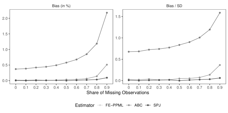
Figure 2: Relative Bias (in %) and Bias / SD of $\hat{\beta}$ for Different $\psi$

Notes: Figure shows relative biases (in %) and ratios of bias to standard deviation for different estimators for $\beta$: uncorrected FE-PPML, analytically corrected ABC, and split-panel jackknife corrected SPJ. $N=200$, $T=5$, and $\psi\in\{0,0.1,\ldots,0.8,0.9\}$. Results are based on $10{,}000$ simulated samples for each $\psi$.

Figure 2 summarizes the results. We find that biases increase with $\psi$, which is to be expected, given the heuristic, as the average number of trading countries ($\overline{N}$) decreases. Furthermore, the biases also increase relative to the dispersion of the estimators, which means that the centering of the standardized estimator, and thus the inference, gets worse as $\psi$ increases. The results demonstrate the importance of identifying latent unbalancedness in empirical work.

Concluding Remarks

We pointed out the relevance of latent unbalancedness for pseudo-poisson estimation of three-way gravity models. Researchers who are unaware of latent unbalancedness and thus rely on the initial sample size to assess the severity of the inference problem - recently shown by WZ - may be misled and mistakenly decide against using bias-corrected estimators. Latent unbalancedness appears to be especially prevalent in sparse networks, e.g. when analysing highly dis-aggregated trade flows as in the empirical application of WZ. Moreover, latent unbalancedness is clearly not only a problem for three-way FE-PPML, but also for other fixed effects maximum likelihood estimators. Finally, we should emphasize that our findings also carry over to classical unbalancedness, i.e. unbalancedness due to missing or incomplete observations, and that uninformative observations can also arise from other more complicated separation issues, as recently shown by [2].

Online Supplement for “Latent Unbalancedness in Three-Way Gravity Models”
by Daniel Czarnowske and Amrei Stammann

Appendix A Iterative Algorithm to Detect Uninformative Observations

We present a simple algorithm to detect all uninformative observations based on the definition in Section 2.2. The idea is as follows. We start with the initial sample and then work sequentially through the FOC’s of $\hat{\alpha}_{it}$, $\hat{\gamma}_{jt}$, and $\hat{\eta}_{ij}$. For instance, we compute $s_{it}=\sum_{j}y_{ijt}$ for each exporter-time combination $it$. If $s_{it}>0$, we keep the corresponding exporter-time observations, otherwise ($s_{it}=0$) we drop them. After we worked through all FOC’s, we check for singleton observations and drop them as well. We repeat these steps until we do not find any additional uninformative observation.

Algorithm.

(Detecting Uninformative Observations)

• Set $r=0$ and $n^{r}$ to the initial sample size, i.e. $n^{r}=138{,}610$ in our example. Repeat step 1–5 until $n^{r}=n^{r-1}$, i.e. we do not find any additional uninformative observations.

• For each exporter-time combination $it$, compute the sum of all trade flows $s_{it}$. If $s_{it}=0$, drop all observations of the exporter-time combination $it$, otherwise keep them.

• For each importer-time combination $jt$, compute the sum of all trade flows $s_{jt}$. If $s_{jt}=0$, drop all observations of the importer-time combination $jt$, otherwise keep them.

• For each country pair $ij$, compute the sum of all trade flows $s_{ij}$. If $s_{ij}=0$, drop all observations of country pair $ij$, otherwise keep them.

• Check all exporter-time combinations, importer-time combinations, and country pairs for singleton observations and drop them.

• Set $r=r+1$ and $n^{r}$ to the current sample size.

Appendix B Latent Unbalancedness in Industry-Level Trade Data

Table 1: Sample Sizes and Average Number of Exporters and Importers

Industry	Code	$n^{\ast}$	$n^{\ast}/{n}$	$\overline{I}$	$\overline{J}$
Agriculture	1	78,765	0.568	94	94
Forestry	2	41,707	0.301	50	52
Fishing	5	32,313	0.233	40	42
Coal	10	15,892	0.115	22	32
Metal Ores	13	20,357	0.147	29	32
Other Mining & Quarrying	14	45,933	0.331	55	58
Food & Beverages	15	87,915	0.634	105	105
Tobacco	16	31,256	0.226	38	46
Textiles	17	77,659	0.560	93	93
Apparel	18	71,111	0.513	85	86
Leather Products	19	63,452	0.458	76	77
Wood & Cork Products	20	61,175	0.441	73	74
Paper & Paper Products	21	59,554	0.430	71	74
Printed & Recorded Media	22	62,318	0.450	75	75
Coke & Refined Petroleum	23	52,214	0.377	63	65
Chemicals & Chemical Products	24	86,185	0.622	103	103
Rubber & Plastic Products	25	75,311	0.543	90	91
Non-Metallic Mineral Products	26	66,136	0.477	79	80
Basic Metal Products	27	66,078	0.477	79	80
Fabricated Metal Products (excl. Machinery)	28	76,095	0.549	91	91
Machinery & Equipment n. e. c.	29	85,955	0.620	103	103
Office, Accounting & Computer Equipment	30	65,219	0.471	78	78
Electrical Equipment	31	76,485	0.552	92	92
Communications Equipment	32	71,600	0.517	86	86
Medical & Scientific Equipment	33	72,790	0.525	87	87
Motor Vehicles, Trailers & Semi-trailers	34	73,715	0.532	88	89
Other Transport Equipment	35	57,217	0.413	69	70
Furniture & Other Manufacturing	36	75,156	0.542	90	90
Aggregate	Agg	119,040	0.859	143	143

• Notes: Data taken from the replication package of WZ. Each data set has $n=138{,}610$ observations and includes all bilateral trade flows of $N=167$ countries during years 1995, 2000, 2005, 2010, and 2015 ($T=5$). $n^{\ast}$, $\overline{I}$, and $\overline{J}$ denote the sample size, the average number of exporters and average number of importers after excluding uninformative observations, respectively.

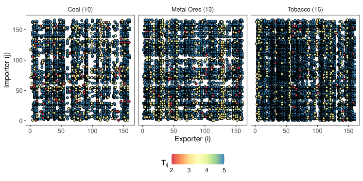
Figure 3: Latent Unbalancedness in Industries 10, 13, and 16

Notes: Data taken from the replication package of WZ. Figure shows patterns of latent unbalancedness in the three most affected industries. Each point indicates a trading country pair. The points differ in color to show how many times we observe the corresponding country pair.

Appendix C Additional Simulation Results

Simulation Evidence – More Detailed Results

Table 2: Simulation Results – $N=200$, $T=5$, and $\psi\in\{0,0.1,\ldots,0.8,0.9\}$

$\psi$	$\overline{N}$	$n$	Bias (in %)			Bias / SD
			FE-PPML	ABC	SPJ	FE-PPML	ABC	SPJ
0.0	200	200,000	0.371	0.016	0.005	0.677	0.029	0.010
0.1	180	180,005	0.385	0.013	0.001	0.684	0.022	0.001
0.2	160	160,005	0.420	0.021	0.005	0.725	0.036	0.009
0.3	140	140,000	0.444	0.010	0.008	0.741	0.017	0.013
0.4	120	120,005	0.493	0.013	0.012	0.774	0.020	0.018
0.5	100	100,005	0.578	0.034	0.000	0.836	0.048	0.000
0.6	80	80,000	0.677	0.040	0.011	0.902	0.052	0.015
0.7	60	60,000	0.848	0.063	0.022	1.008	0.074	0.025
0.8	40	40,005	1.187	0.140	0.034	1.195	0.138	0.033
0.9	20	20,005	2.177	0.512	0.094	1.589	0.366	0.062

• Notes: Table shows relative biases (in %) and ratios of bias to standard deviation for different estimators for $\beta$: uncorrected FE-PPML, analytically corrected ABC, and split-panel jackknife corrected SPJ. Results are based on $10{,}000$ simulated samples for each $\psi$.

Simulation Evidence – Confirm Validity of Heuristic

We conduct a simulation study to confirm the validity of the heuristic proposed by WZ. We first generate balanced panels with $N$ countries trading with each other for $T=5$ periods, i.e. each simulated sample has initially $n=N^{2}T$ observations. Then $\psi N^{2}$ country pairs are dropped randomly so that the final sample has $n^{\ast}=(1-\psi)N^{2}T\approx N\overline{N}T$ observations. We consider different fractions of missing observations $\psi\in\{0,0.1,\ldots,0.8,0.9\}$ and choose $N=\lfloor 20/(1-\psi)\rfloor$ so that $\overline{N}\approx 20$ remains roughly constant over $\psi$. We generate balanced panels following DGP I of WZ,

$$y_{ijt} =\lambda_{ijt}\,\omega_{ijt}\,,$$ (4)

$$x_{ijt} =0.5\,x_{ijt-1}+\alpha_{it}+\gamma_{jt}+\eta_{ij}+\nu_{ijt}\,,$$

$$\omega_{ijt} =\exp(-0.5\,\log(1+\lambda_{ijt}^{-2})+(\log(1+\lambda_{ijt}^{-2}))^{-0.5}\,z_{ijt})\,,$$

$$z_{ijt} =0.3\,z_{ijt-1}+\xi_{ijt}\,,$$

where $i,j\in\{1,\ldots,N\}$, $t\in\{1,\ldots,T\}$, $\lambda_{ijt}=\exp(\beta\,x_{ijt}+\alpha_{it}+\gamma_{jt}+\eta_{ij})$, $\alpha_{it}$, $\gamma_{jt}$, and $\eta_{ij}$ are $\sim\operatorname{\text{iid.}\;}\operatorname{\mathcal{N}}(0,0.25)$, $\nu_{ijt}\sim\operatorname{\text{iid.}\;}\operatorname{\mathcal{N}}(0,\sqrt{0.5})$, $x_{ij0}=\eta_{ij}+\nu_{ij0}$, $z_{ij0}\sim\operatorname{\text{iid.}\;}\operatorname{\mathcal{N}}(0,1)$, $\xi_{ijt}\sim\operatorname{\text{iid.}\;}\operatorname{\mathcal{N}}(0,0.91)$, and $\operatorname{\mathcal{N}}(a,b)$ denotes the normal distribution with mean $a$ and variance $b$. We set $\beta=1$ and consider the same estimators for $\beta$ as WZ: an uncorrected estimator (FE-PPML), an analytically bias-corrected estimator (ABC), and a split-panel jackknife bias-corrected estimator (SPJ). Our results are based on $10{,}000$ simulated samples for each $\psi$.

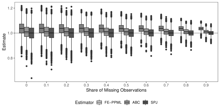
Figure 4: Estimates for $\beta$ for Different $\psi$

Notes: Figure shows boxplots of estimates for $\beta$ from different estimators: uncorrected FE-PPML, analytically corrected ABC, and split-panel jackknife corrected SPJ. Results are based on $10{,}000$ simulated samples for each $\psi$.

Figure 4 summarizes the results. As predicted by the heuristic, we find that the biases remain constant over $\psi$, i. e. depend on the average number of trading countries ($\overline{N}$). Furthermore, we find that increasing $\psi$ decreases the dispersion of the estimators, as indicated by the boxes becoming narrower. This was to be expected since the sample size $n^{\ast}$ grows with $\psi$. However, this also means that inference gets worse as $\psi$ increases, since biases increase relative to the dispersion of the estimators. In other words, confidence intervals constructed around the estimators become narrower without any improvement in their centering by increasing the sample size.

References

- [1] Adelin Albert and John A. Anderson “On the existence of maximum likelihood estimates in logistic regression models” In Biometrika 71.1, 1984, pp. 1–10
- [2] Sergio Correia, Paulo Guimarães and Thomas Zylkin “Verifying the existence of maximum likelihood estimates for generalized linear models” In arXiv preprint arXiv:1903.01633, 2021
- [3] C. Gourieroux, A. Monfort and A. Trognon “Pseudo Maximum Likelihood Methods: Theory” In Econometrica 52.3, 1984, pp. 681–700
- [4] Keith Head and Thierry Mayer “Chapter 3 - Gravity Equations: Workhorse,Toolkit, and Cookbook” In Handbook of International Economics 4, Handbook of International Economics Elsevier, 2014, pp. 131–195
- [5] JMC Santos Silva and Silvana Tenreyro “The log of gravity” In The Review of Economics and Statistics 88.4, 2006, pp. 641–658
- [6] JMC Santos Silva and Silvana Tenreyro “On the existence of the maximum likelihood estimates in Poisson regression” In Economics Letters 107.2, 2010, pp. 310–312
- [7] Martin Weidner and Thomas Zylkin “Bias and consistency in three-way gravity models” In Journal of International Economics 132, 2021, pp. 103513