Cluster-Robust Estimators for Bivariate Mixed-Effects Meta-Regression

Abstract

Meta-analyses frequently include trials that report multiple effect sizes based on a common set of study participants. These effect sizes will generally be correlated. Cluster-robust variance-covariance estimators are a fruitful approach for synthesizing dependent effects. However, when the number of studies is small, state-of-the-art robust estimators can yield inflated Type 1 errors. We present two new cluster-robust estimators, in order to improve small sample performance. For both new estimators the idea is to transform the estimated variances of the residuals using only the diagonal entries of the hat matrix. Our proposals are asymptotically equivalent to previously suggested cluster-robust estimators such as the bias reduced linearization approach. We apply the methods to real world data and compare and contrast their performance in an extensive simulation study. We focus on bivariate meta-regression, although the approaches can be applied more generally.

Keywords: Meta-regression, multivariate analysis, cluster-robust estimators, Monte-Carlo-simulation

1 Introduction

In psychometric and medical research, studies frequently report multiple dependent outcomes. These effects can be synthesized across studies, while incorporating study level moderators, via multivariate meta-regression (Berkey et al.,, 1998). This is a more sophisticated approach than averaging the effects within studies to create aggregate effects, which are then synthesized. A fruitful approach to achieve reliable inference in the case of a multivariate meta-regression is to use a cluster-robust (CR) variance-covariance estimator (Hedges et al.,, 2010). Robust estimators are designed to account for potential model misspecification. They can handle dependent effect size estimates and heteroscedastic model errors. A frequent problem in multivariate meta-analysis models is that it is difficult to impossible to compute the variance-covariance matrix of the vector of effect estimates. This is because trials frequently report neither the sampling covariances between study effects nor individual patient data (IPD). This is where CR estimators come into play: They have multiple advantages, such as providing consistent standard errors and asymptotically valid tests without requiring restrictive assumptions regarding the (correlation) structure of the model errors.

Cluster-robust estimators are an extension of heteroscedasticity consistent $(HC)$ estimators. $HC$ estimators, proposed by White, (1980) and later extended in Cribari-Neto, (2004) and Cribari-Neto et al., (2007), were first proposed in the meta-analytic literature by Sidik and Jonkman, (2005). They have been examined and applied for use in ANCOVA (Zimmermann et al.,, 2019), ordinary least squares regression (Hayes and Cai,, 2007) and mixed-effect meta-regression (Hedges et al.,, 2010; Viechtbauer et al.,, 2015; Welz and Pauly,, 2020). When trials report multiple effects stemming from the same study participants, their clustered, i.e. correlated nature should be accounted for. This is where CR estimators come in. The original formulations of both HC and CR estimators have been shown to possess a downward bias for variance components, as well as yielding highly inflated Type 1 errors of respective test procedures in case of a small number of studies/clusters (Viechtbauer et al.,, 2015; Tipton and Pustejovsky,, 2015; Welz and Pauly,, 2020). Therefore it is recommended to instead use one of various improvements that have been suggested. We discuss some of these, such as the bias reduced linearization approach and $CR_{3}$ as introduced in Bell and McCaffrey, (2002), as well as two new proposals in the chapter on cluster-robust estimators. These can be applied generally for multivariate meta-regression, but we focus specifically on the bivariate case.

First, we present the statistical model, as well as tests and confidence regions for the model coefficients in Section 2. In Section 3, we describe multiple CR estimators, including two new suggestions. In Section 4, we conduct a real world data analysis. Section 5 describes the design and results of our simulation study. We close with a discussion of the results and an outlook for future research (Section 6).

2 The Set-up

The usual multivariate mixed-effects meta-regression model (Jackson et al.,, 2011) is given by

$$\boldsymbol{Y_{i}}=\boldsymbol{X_{i}\beta+u_{i}+\varepsilon_{i}},\ i=1,\ldots,l,$$ (1)

where $k$ is the number of independent studies, $\boldsymbol{\beta}\in\mathbb{R}^{q}$ is a vector of coefficients and $\boldsymbol{X_{i}}$ a $p_{i}\times q$ design matrix of study-level covariates. In the following we will assume that there are $p$ effects of interest per study, but only $p_{i}\leq p$ effects are observed (reported) in study $i$, i.e. $\boldsymbol{Y_{i}}\in\mathbb{R}^{p_{i}}$. Furthermore, $\boldsymbol{u_{i}}$ is a random effect that is typically assumed to be multivariate normally distributed with $\boldsymbol{u_{i}}\sim\mathcal{N}(\boldsymbol{0,T_{i}})$ and $\boldsymbol{\varepsilon_{i}}$ is the within-study error with $\boldsymbol{\varepsilon_{i}}\sim\mathcal{N}(\boldsymbol{0,V_{i}})$. With $\boldsymbol{T_{i}}$ we refer to the $p_{i}\times p_{i}$ submatrix of the matrix $\boldsymbol{T}=\begin{pmatrix}\tau_{1}^{2}&\tau_{12}\\ \tau_{12}&\tau_{2}^{2}\end{pmatrix}$, denoting the $p\times p$ between-study variance-covariance matrix (under complete data). $\boldsymbol{V_{i}}$ refers to the corresponding $p_{i}\times p_{i}$ within-study variance-covariance matrix. A typical example would be a compound symmetry structure for $\boldsymbol{T_{i}}$, see Section 5 below. We rewrite model (1) in matrix notation as

$$\boldsymbol{Y=X\beta+u+\varepsilon},$$ (2)

with $\boldsymbol{\beta}\in\mathbb{R}^{q}$, $\boldsymbol{Y=(Y_{1}^{\prime},\ldots,Y_{K}^{\prime})^{\prime}}$, and design matrix X. Assuming that we have a block diagonal matrix of weights $\boldsymbol{\widehat{W}}=\text{diag}(\boldsymbol{\widehat{W}}_{1},\ldots,\boldsymbol{\widehat{W}}_{K})$, usually corresponding to the inverse variance weights with $\boldsymbol{\widehat{W}_{i}}=\left(\boldsymbol{\widehat{T}_{i}+V_{i}}\right)^{-1}$, then the weighted least squares estimator for $\boldsymbol{\beta}$ is given by (Hedges et al.,, 2010)

$$\boldsymbol{\hat{\beta}=(X^{\prime}\widehat{W}X)^{-1}X^{\prime}\widehat{W}Y}.$$ (3)

We will focus on constructing (multivariate) confidence regions for $\boldsymbol{\beta}$ and confidence intervals for the individual coefficients $\beta_{j},\ j=1,\ldots,q$ based on testing the hypotheses $H_{0}:\{\boldsymbol{\beta}=\boldsymbol{\beta}_{0}\}$ vs. $H_{1}:\{\boldsymbol{\beta}\neq\boldsymbol{\beta}_{0}\}$. We set $\boldsymbol{\Sigma}=\text{Cov}(\boldsymbol{\hat{\beta}})$ and denote estimates thereof by $\boldsymbol{\widehat{\Sigma}}$. We discuss specific choices for estimating $\boldsymbol{\Sigma}$ in Section 3.

Neglecting multiplicity, we note that a commonly used confidence interval for $\beta_{j},\ j=1,\ldots,q$ is given by

$$\hat{\beta}_{j}\pm\sqrt{\boldsymbol{\widehat{\Sigma}}_{jj}}z_{1-\alpha/2}.$$ (4)

Here $z_{1-\alpha/2}$ denotes the $1-\alpha/2$ quantile of the standard normal distribution and $\widehat{\boldsymbol{\Sigma}}_{jj}$ denotes the $j^{th}$ diagonal element of $\widehat{\boldsymbol{\Sigma}}$. A confidence interval with better small sample performance that is asymptotically equivalent for $k\rightarrow\infty$ is given by using the $t_{p(k)-q,1-\alpha/2}$ quantile instead, which refers to the $1-\alpha/2$ quantile of the $t$-distribution with $p(k)-q$ degrees of freedom. Here $p(k)\coloneqq\sum_{i=1}^{k}p_{i}$ is the total number of observed effects, which is equal to the number of studies $k$ in the univariate setting (Viechtbauer et al.,, 2015). Alternatively the degrees of freedom of the $t$ distribution can be estimated via a Satterthwaite approximation, as suggested by Bell and McCaffrey, (2002).

In order to construct a $(1-\alpha)$ confidence region for $\boldsymbol{\beta}$ we consider the usual Wald-type test-statistic (Tipton and Pustejovsky,, 2015)

$$Q=(\boldsymbol{\hat{\beta}}-\boldsymbol{\beta}_{0})^{\prime}\widehat{\boldsymbol{\Sigma}}^{-1}(\boldsymbol{\hat{\beta}}-\boldsymbol{\beta}_{0}),$$ (5)

Alternatively, if one were interested in testing more general hypotheses of the form $H_{0}:\{\boldsymbol{H}\boldsymbol{\beta}=\boldsymbol{c}\}$ vs. $H_{1}:\{\boldsymbol{H}\boldsymbol{\beta}\neq\boldsymbol{c}\}$ for some hypothesis matrix $\boldsymbol{H}\in\mathbb{R}^{s\times q}$ (which we assume to be of full rank) and vector $\textbf{c}\in\mathbb{R}^{s}$, then the test statistic becomes

$$Q_{\boldsymbol{H}}=(\boldsymbol{H}\boldsymbol{\hat{\beta}}-\boldsymbol{c})^{\prime}(\boldsymbol{H}\widehat{\boldsymbol{\Sigma}}\boldsymbol{H}^{\prime})^{-1}(\boldsymbol{H}\boldsymbol{\hat{\beta}}-\boldsymbol{c}),$$

For example, the special case of a test regarding a single regression coefficient $\beta_{a}$ would be given by $\boldsymbol{H}$ equal to a vector of length $q$ with a 1 at entry $a$ and 0 otherwise.

Under the null hypothesis $Q$ is approximately $\chi^{2}_{q}$-distributed (and $Q_{\boldsymbol{H}}$ approximately $\chi^{2}_{f}$-distributed with $f=\text{rank}(\boldsymbol{H})$), assuming $\boldsymbol{\Sigma}$ is positive definite. However, it is known that tests based on this approximation can perform poorly for small to moderate values of $k$ (Tipton and Pustejovsky,, 2015). An arguably better alternative is the $F$-test

$$\mathds{1}\left\{Q>qF_{q,k-q,1-\alpha}\right\},$$ (6)

where $F_{q,k-q,1-\alpha}$ denotes the $1-\alpha$ quantile of an $F$-distribution with $q$ and $k-q$ degrees of freedom. This is analogous to the $t$-tests for univariate coefficients and is superior to the test based on the asymptotic $\chi^{2}$-approximation (Tipton and Pustejovsky,, 2015). However, the $F$-test has been criticized for only performing well in certain scenarios (Tipton,, 2015). As a remedy for smaller $k$, Tipton and Pustejovsky, (2015) proposed to approximate $Q$ by a Hotelling’s $T^{2}$ distribution with parameters $q$ and (degrees of freedom) $\eta$, such that

$$\frac{\eta-q+1}{\eta q}Q\sim F(q,\eta-q+1).$$ (7)

They discuss different approaches for estimating the degrees of freedom $\eta$. Based on their research, they recommend an estimation approach, which they call “HTZ”. We briefly summarize this estimator, originally proposed by Zhang, (2012) for heteroscedastic one-way MANOVA, and refer to their paper for details.

First note that the statistic in (5) can also be written as $Q=\boldsymbol{z}^{\prime}\boldsymbol{S}^{-1}\boldsymbol{z}$ with $\boldsymbol{z}=\boldsymbol{\Sigma}^{-1/2}(\boldsymbol{\hat{\beta}}-\boldsymbol{\beta}_{0})$ and $\boldsymbol{S}=\boldsymbol{\Sigma}^{-1/2}\boldsymbol{\widehat{\Sigma}}\boldsymbol{\Sigma}^{-1/2}$. Under $H_{0}$, $\boldsymbol{z}$ is normally distributed with mean $\boldsymbol{0}$ and covariance $\boldsymbol{I}$ (Tipton and Pustejovsky,, 2015). Moreover, if $\boldsymbol{S}$ is a random $q\times q$ matrix such that $\eta\boldsymbol{S}$ follows a Wishart distribution with $\eta$ degrees of freedom and scale matrix $\boldsymbol{I}_{q}$, the estimator is given by

$$\hat{\eta}_{Z}=\frac{q(q+1)}{\sum_{a=1}^{q}\sum_{b=1}^{q}\text{Var}(s_{ab})}.$$

Here $s_{ab}$ denotes the entry $(a,b)$ of $\boldsymbol{S}$. This approach corresponds to setting the total variation in $\boldsymbol{S}$ equal to the total variation in a Wishart distribution (Tipton and Pustejovsky,, 2015).

However, our own simulations showed that there are situations when $\hat{\eta}_{Z}<q-1$ and therefore $\hat{\eta}_{Z}-q+1<0$. Specifically this frequently happened in cases with a small number of studies ($k\leq 5$). As the degrees of freedom in an $F$ distribution cannot be negative the HTZ approach is not applicable here. Therefore we will stick to the classical $F$-test (6), although we propose a small sample adjustment. In our simulations the $F$-test (6) leads to very liberal or conservative results, depending on the variance-covariance estimator used, in settings with $k=5$ studies. We therefore propose to truncate the denominator degrees of freedom at the value two, i.e. we consider the $F$-test

$$\mathds{1}\left\{Q>qF_{q,\max(2,k-q),1-\alpha}\right\}.$$ (8)

The simple motivation behind this adjustment is that for an $F_{m,n}$ distribution with degrees of freedom $m$ and $n$ the expected value $\frac{n}{n-2}$ only exists when $n>2$. We also tested a truncation of the denominator degrees of freedom at three. However, simulations indicate superior coverage of respective confidence intervals for a truncation at two.

Confidence regions for $\boldsymbol{\beta}$ can be derived via test inversion. For example, if (8) is a test for $H_{0}:\{\boldsymbol{\beta=\beta_{0}}\}$ vs. $H_{1}:\{\boldsymbol{\beta\neq\beta_{0}}\}$, then the set

$$\Lambda:=\left\{\boldsymbol{\beta}\in\mathbb{R}^{q}:(\boldsymbol{\hat{\beta}}-\boldsymbol{\beta})^{\prime}\widehat{\boldsymbol{\Sigma}}^{-1}(\boldsymbol{\hat{\beta}}-\boldsymbol{\beta})\leq qF_{q,\max(2,k-q),1-\alpha}\right\}$$ (9)

is a corresponding confidence region for $\boldsymbol{\beta}$.

A confidence ellipsoid can be obtained following Johnson et al., (2014), based on the eigenvalues $\hat{\lambda}_{j}$ and eigenvectors $\boldsymbol{\hat{e}}_{j}$ of $\widehat{\boldsymbol{\Sigma}}$. This means $\Lambda$ is an ellipsoid centered around $\boldsymbol{\hat{\beta}}$, whose axes are given by

$$\boldsymbol{\hat{\beta}}\pm\sqrt{\hat{\lambda}_{j}qF_{q,\max(2,k-q),1-\alpha}}\boldsymbol{\hat{e}}_{j},\ \ j=1,\ldots,q.$$

This means $\Lambda$ extends for $\sqrt{\hat{\lambda}_{j}qF_{q,\max(2,k-q),1-\alpha}}$ units along the estimated eigenvector $\boldsymbol{\hat{e}}_{j}$ for $j=1,\ldots,q$. Since the volume of an $n$-dimensional ellipsoid with axis lengths $a_{1},\ldots,a_{n}$ is given by (Wilson,, 2010)

$$V=\frac{2\pi^{n/2}}{n\Gamma(n/2)}\prod_{i=1}^{n}a_{i},$$

the volume of the confidence ellipsoid $\Lambda$ is equal to

$$V_{\Lambda}=\frac{2\pi^{q/2}}{q\Gamma(q/2)}\prod_{i=1}^{q}\sqrt{\hat{\lambda}_{i}qF_{q,\max(2,k-q),1-\alpha}}.$$

3 Cluster-Robust Covariance Estimators

Robust variance-covariance estimators, also known as sandwich estimators or Huber-White estimators, have been recommended as a promising alternative in the context of meta-regression (Hedges et al.,, 2010; Tipton,, 2015; Welz and Pauly,, 2020). Robust estimators are designed to account for potential model misspecification. They have many desirable properties, such as consistency under heteroscedasticity or asymptotic normality (Hedges et al.,, 2010) without making restrictive assumptions about the specific form of the effect sizes’ sampling distributions.

The reliability of confidence regions based on the statistic (5) depends on the quality of the estimator $\widehat{\boldsymbol{\Sigma}}$ for $\boldsymbol{\Sigma}=\text{Cov}(\boldsymbol{\hat{\beta}})$. The standard (Wald-type) estimator, which we will refer to as $ST$, is given by $(\boldsymbol{X^{\prime}\widehat{W}X})^{-1}$. The motivation behind this estimator is that the true covariance matrix of $\boldsymbol{\widehat{\beta}}$ (given correct weights) is equal to $\boldsymbol{\Sigma}=(\boldsymbol{X^{\prime}WX})^{-1}$ with $\boldsymbol{W}=\text{diag}\left(\boldsymbol{W_{1}},\ldots,\boldsymbol{W_{K}}\right)$ and $\boldsymbol{W_{i}}=\boldsymbol{T_{i}+V_{i}}$. However, this ignores the imprecision in the estimation of $\boldsymbol{T,V}$ and therefore in the estimation of W. In fact, if $\boldsymbol{T}$ is estimated poorly, this may lead to deviations from nominal Type 1 error and coverage of corresponding confidence regions (Sidik and Jonkman,, 2005).

In the case of univariate meta-analysis and meta-regression heteroscedasticity-consistent (HC) estimators can be applied (Sidik and Jonkman,, 2005; Viechtbauer et al.,, 2015; Welz and Pauly,, 2020). For multivariate meta-regression however, the correlated nature of the study effects needs to be taken into account. We therefore consider cluster-robust (CR) estimators. A selection of CR estimators is, e.g., implemented in the R package clubSandwich (Pustejovsky,, 2021). The package recommendation is the “bias reduced linearization” approach $CR_{2}$, which is discussed in detail in Tipton and Pustejovsky, (2015); Pustejovsky and Tipton, (2018). Sandwich estimators (of HC- as well as CR-type) are all of the general form

$$\widehat{\boldsymbol{\Sigma}}=\boldsymbol{(X^{\prime}\widehat{W}X)^{-1}X^{\prime}\widehat{W}\widehat{\Omega}\widehat{W}X(X^{\prime}\widehat{W}X)^{-1}},$$ (10)

with the differences lying in the central “meat” matrix $\widehat{\boldsymbol{\Omega}}$, surrounded by the “bread”. This form motivates the name “sandwich” estimator. $HC_{1}$ is arguably the best known sandwich estimator in the context of univariate meta-regression (Hedges et al.,, 2010; Viechtbauer et al.,, 2015; Tipton and Pustejovsky,, 2015). However, the extensions $HC_{3}$ and $HC_{4}$ are frequently recommended as superior alternatives in the non meta-analytic literature, see Cribari-Neto et al., (2007) for details, and have been shown to be superior to $HC_{1}$ (Long and Ervin,, 2000; Hayes and Cai,, 2007; Zimmermann et al.,, 2019). A natural extension of $HC_{1}$ for the multivariate setting and what we will refer to as $CR_{1}^{*}$ is defined as

$$\widehat{\boldsymbol{\Sigma}}_{CR_{1}^{*}}=\tfrac{k}{k-q}\boldsymbol{(X^{\prime}\widehat{W}X)^{-1}\left(\sum_{i=1}^{K}X_{i}^{\prime}\widehat{W}_{i}\widehat{\Omega}_{i}\widehat{W}_{i}X_{i}\right)(X^{\prime}\widehat{W}X)^{-1}},$$ (11)

where $\widehat{\boldsymbol{\Omega}}_{i}=\boldsymbol{E_{i}E_{i}^{\prime}}$ with $\boldsymbol{E_{i}}=\boldsymbol{Y_{i}-X_{i}\hat{\beta}}$ and $\frac{k}{k-q}$ is a correction factor that converges to 1 as $k$ goes to infinity. The motivation for this factor is to correct for a liberal behavior in case of few studies/clusters $k$; see the clubSandwich package for similar choices.

However, as our simulation study below will show, tests based on $CR_{1}^{*}$ are still quite liberal when $k$ is small. An alternative is to instead use a bias reduced linearization approach, which was originally proposed by Bell and McCaffrey, (2002) and further developed by Pustejovsky and Tipton, (2018). This estimator, called $CR_{2}$, is designed to be exactly unbiased under the correct specification of a working model. This is achieved via a clever choice of adjustment matrices in the formulation of the estimator, see Tipton and Pustejovsky, (2015); Pustejovsky and Tipton, (2018) for details. This is the recommended approach in the clubSandwich package (Pustejovsky,, 2021). Another alternative is the $CR_{3}$ estimator, which is a close approximation of the leave-one-(cluster)-out Jackknife variance-covariance estimator. $CR_{3}$ is also implemented in the clubSandwich package.

However, all of the estimators above can be unsatisfactory for small $k$, as our simulations will show. Therefore, in addition to these $CR$-estimators, we propose two others, which are extensions of the $HC_{3}$ and $HC_{4}$ estimators. Since $HC_{3}$ and $HC_{4}$ often outperform both $HC_{1}$ and $HC_{2}$ in the univariate regression setting (Long and Ervin,, 2000; Cribari-Neto,, 2004; Welz and Pauly,, 2020), one would suspect their respective cluster-robust extensions to outperform in the case of multivariate regression. We therefore define $CR_{3}^{*}$ and $CR_{4}^{*}$ via

$$\widehat{\boldsymbol{\Sigma}}_{CR_{3}^{*}}=\boldsymbol{(X^{\prime}\widehat{W}X)^{-1}\left(\sum_{i=1}^{K}X_{i}^{\prime}\widehat{W}_{i}\widehat{\Omega}_{3i}\widehat{W}_{i}X_{i}\right)(X^{\prime}\widehat{W}X)^{-1}},$$ (12)

$$\widehat{\boldsymbol{\Sigma}}_{CR_{4}^{*}}=\boldsymbol{(X^{\prime}\widehat{W}X)^{-1}\left(\sum_{i=1}^{K}X_{i}^{\prime}\widehat{W}_{i}\widehat{\Omega}_{4i}\widehat{W}_{i}X_{i}\right)(X^{\prime}\widehat{W}X)^{-1}}.$$ (13)

Here $\widehat{\boldsymbol{\Omega}}_{3i}$ is defined as

$$\widehat{\boldsymbol{\Omega}}_{3i}=\widehat{\boldsymbol{\Omega}}_{i}-\Delta+\Delta\cdot\left(\boldsymbol{I}_{p_{i}}-\text{diag}(\boldsymbol{H}_{i})\right)^{-2},$$ (14)

where $\boldsymbol{H}_{i}$ refers to the submatrix of $\boldsymbol{H}$ with entries pertaining to study $i$, $p_{i}$ is the number of observed effects in study $i$ and $\Delta=\text{diag}(\boldsymbol{E_{i}E_{i}^{\prime}})$. $\boldsymbol{H}$ refers to the hat matrix $\boldsymbol{H}=\boldsymbol{X(X^{\prime}\widehat{W}X)^{-1}X^{\prime}\widehat{W}}$. Furthermore, $\widehat{\boldsymbol{\Omega}}_{4i}$ is equal to (14) except $\Delta$ is multiplied with $\left(\boldsymbol{I}_{p_{i}}-\text{diag}(\boldsymbol{H}_{i})\right)^{-\delta_{i}}$, where $\delta_{i}=\min\left\{4,h_{ii}/\bar{h}\right\}$ with $h_{ii}$ denoting the $i$-$th$ diagonal element of $\boldsymbol{H}$ and $\bar{h}$ is the average of the values in the diagonal of the hat matrix. This data-dependent exponent stems from the $HC_{4}$ suggestion by Cribari-Neto, (2004). $HC_{4}$ performs well in univariate meta-regression (Welz and Pauly,, 2020) and therefore motivates an extension to the cluster-robust context.

We highlight that our proposed estimator $CR_{3}^{*}$ is different from the estimator $CR_{3}$ implemented in the R package clubSandwich as proposed by Bell and McCaffrey, (2002). Whereas the latter uses the entire hat matrix for each cluster, we propose to use just the diagonal elements. In contrast, the “meat” matrix for $CR_{3}$ is given by $\sum_{i=1}^{K}\boldsymbol{X_{i}^{\prime}\widehat{W}_{i}(I-H_{i})^{-1}\widehat{\Omega}_{i}(I-H_{i})^{-1}\widehat{W}_{i}X_{i}}$. Furthermore note that $CR_{3}^{*}$ is not even equal to the estimator with meat matrix given by

$$\sum_{i=1}^{K}\boldsymbol{X_{i}^{\prime}\widehat{W}_{i}(I-\text{diag}(H_{i}))^{-1}\widehat{\Omega}_{i}(I-\text{diag}(H_{i}))^{-1}\widehat{W}_{i}X_{i}}$$

because $\boldsymbol{\widehat{\Omega}_{i}}$ is in general not a diagonal matrix (only block-diagonal), due to the clustered nature of the data.

For univariate regression we were able to prove the asymptotic equivalence of all $HC$ estimators, which is formulated in the supplement of Welz and Pauly, (2020). Under some some weak regularity conditions it follows that the leverages asymptotically converge to zero, as the number of studies $k$ goes to infinity. Therefore, we expected similar results to hold for $CR$ estimators with analogous arguments. A theorem regarding the asymptotic equivalence of $CR$ estimators under regularity conditions is given in the supplement of this paper, along with a proof.

4 Data Analysis

We exemplify the methods presented in this manuscript with the analysis of a dataset containing 81 trials examining overall (OS) and/or disease-free survival (DFS) in neuroblastoma patients with amplified (extra copies) versus normal MYC-N genes. The data are contained in the R package metafor and were previously analyzed by Riley et al., (2003, 2007). Amplified MYC-N levels are associated with poorer outcomes. The effect measures are log hazard ratios with positive values indicating an increased risk of death or relapse/death for patients with higher MYC-N levels as compared to patients with lower levels. 17 studies reported both outcomes, 25 studies only reported DFS and 39 studies only reported OS.

The dataset contains the log hazard ratios and the corresponding sampling variances. However, since no information is available on the sampling covariances between OS and DFS we must make some assumptions with regard to our working model. In the spirit of a sensitivity analysis we will first assume a weaker correlation of $\varrho_{1}=0.5$ and subsequently a stronger correlation of $\varrho_{2}=0.8$ and then compare the results. This means for a hypothetical study $i$ that reports log hazard ratios for OS and DFS, $y_{i,OS}$ and $y_{i,DFS}$, with an assumed correlation of 0.5 along with respective sampling variances $\sigma_{i,OS}^{2}$ and $\sigma_{i,DFS}^{2}$, we have the sampling variance-covariance matrix $V_{i}=\begin{pmatrix}\sigma_{i,OS}^{2}&0.5\cdot\sigma_{i,OS}\sigma_{i,DFS}\\ 0.5\cdot\sigma_{i,OS}\sigma_{i,DFS}&\sigma_{i,DFS}^{2}\end{pmatrix}$.

We assume a multivariate meta-regression model that includes a random effect as in Section 2 as well as an unstructured (but positive definite) variance-covariance matrix. In the following we are interested in testing whether both pooled effects are different from zero. When the full dataset is analyzed, the Wald-test for $H_{0}:\{\boldsymbol{\beta=0}\}$ vs. $H_{1}:\{\boldsymbol{\beta\neq 0}\}$ returns a p-value $<0.001$ for all CR estimators and for both $\varrho_{1}$ and $\varrho_{2}$. However, let us assume we only had the data from studies 1-5, which all contain results for both OS and DFS. Such a situation is not unrealistic, considering the median number of studies per meta-analyses in a sample of 22,453 published meta-analyses from the Cochrane Database was three (Davey et al.,, 2011). This reduced dataset is shown in Table 1. The p-values for the estimators $CR_{1}*$, $CR_{3}*$, $CR_{4}*$, $CR_{2}$ and $ST$ for assumed correlations $\varrho_{1},\ \varrho_{2}$ are displayed in Table 2.

study	$y_{i}$	$v_{i}$	outcome
1	-0.11	0.45	DFS
1	-0.14	0.66	OS
2	0.30	0.07	DFS
2	0.67	0.08	OS
3	0.41	0.77	DFS
3	0.43	0.66	OS
4	0.47	0.29	DFS
4	2.08	0.45	OS
5	0.76	0.24	DFS
5	0.70	0.31	OS

Table 1: Sample of five studies containing log hazard ratios ($y_{i}$) for disease-free and overall survival and their respective sampling variances ($v_{i}$).

The results show that when the number of studies is small the p-values can vary substantially, depending on the choice of estimator. Furthermore, the results based on CR estimators appear to be more stable and depend much less on the underlying $\boldsymbol{V}$ matrix i.e. the assumed correlation between OS and DFS than the standard estimator $\boldsymbol{(X^{\prime}\widehat{W}X)^{-1}}$. This motivates the use of a CR approach over the standard variance-covariance estimator.

Estimators	p-values
	$\varrho_{1}$	$\varrho_{2}$
CR1*	0.073	0.075
CR3*	0.069	0.077
CR4*	0.076	0.090
CR2	0.054	0.055
ST	0.138	0.206

Table 2: p-values of Wald-tests based on CR estimators and the standard variance-covariance estimator $\boldsymbol{(X^{\prime}\widehat{W}X)^{-1}}$ for assumed correlations of $\varrho_{1}=0.5$ and $\varrho_{2}=0.8$.

5 Simulation Study

Simulation Design In order to assess the performance of the previously discussed methods, we conducted a Monte Carlo simulation. We considered $k\in\{5,10,20,40\}$ studies, average study sizes $N\in\{40,100\}$ with balanced treatment and control groups, coefficient vectors $\boldsymbol{\beta}=(\beta_{0},\beta_{1},\beta_{2},\beta_{3})^{\prime}\in\{(0,0,0,0)^{\prime},(0.2,0.2,0.1,0.1)^{\prime},(0.4,0.4,0.2,0.3)^{\prime}\}$, correlations $\varrho\in\{0,0.3,0.7\}$ and missing data ratios from $\{0,0.1,0.2,0.3,0.4\}$. The latter refers to the number of studies that only report one of the two effects of interest and $\varrho$ refers to the IPD correlations between the two observed outcomes. In the coefficient vector $\boldsymbol{\beta}$ the first two entries refer to the population means of the two effects of interest and the other two represent the effect of the study-level moderator on each effect respectively. Study sizes were varied, such that for an average study size $N$, $20\%$ of studies had size $0.8N,0.9N,\ldots,1.2N$ respectively. Datasets with missing data were generated by first simulating complete data and then removing entries completely at random.

The simulated study-level effects are (correlated) standardized mean differences (SMD). We estimated these SMDs via the adjusted Hedges’ $g$ (Hedges,, 1981)

$$g\coloneqq\frac{\Gamma(m/2)}{\sqrt{(m/2)}\Gamma((m-1)/2)}d$$

with $m=n_{T}+n_{C}-2$ and where $n_{T}$ and $n_{C}$ refer to the treatment and control group sizes. Hedges’ $g$ is defined as $d=(\bar{x}_{T}-\bar{x}_{C})/s^{*}$, with a pooled standard deviation $s^{*}=\sqrt{\frac{(n_{T}-1)s_{T}^{2}+(n_{C}-1)s_{C}^{2}}{m}}$, where $s_{T}^{2},s_{C}^{2}$ refer to the variances in the treatment and control groups respectively (Hedges,, 1981). This adjustment to Hedges’ $g$ yields an unbiased effect estimator (Lin and Aloe,, 2021). We generated the SMDs by first simulating individual participant data (IPD). The treatment and control group IPD observations $Y_{ij}^{T}$ and $Y_{ij}^{C}$ were drawn from bivariate normal distributions respectively. More precisely, for study $i=1,\ldots,k$ and participant $j=1,\ldots,N_{i}/2$ the observations are drawn from $Y_{ij}^{T}\sim\mathcal{N}(\theta_{i},P)$ and $Y_{ij}^{C}\sim\mathcal{N}(\boldsymbol{0},P)$ with $\theta_{i}=\boldsymbol{X\beta+u_{i}}$ and $P=\begin{pmatrix}1&\varrho\\ \varrho&1\end{pmatrix}$ is the population correlation matrix of the outcomes in study $i$. $\boldsymbol{X}$ is a $2\times q$ design matrix of covariates. In our specific simulation design of a single study-level covariate $x$ with potentially different influence on the two study effects we have $\boldsymbol{X}=\begin{pmatrix}1&0&x&0\\ 0&1&0&x\end{pmatrix}$.

For the heterogeneity matrix $\boldsymbol{T}$ we consider the two settings

$$\begin{pmatrix}\tau^{2}&0.2\tau^{2}\\ 0.2\tau^{2}&\tau^{2}\end{pmatrix}\text{and }\begin{pmatrix}\tau^{2}&0.4\tau^{2}\\ 0.4\tau^{2}&2\tau^{2}\end{pmatrix}.$$

For $M=N/2$ (average size of the treatment and control groups), we set $\tau^{2}:=\frac{2}{M}+\frac{\beta_{0}^{2}}{4M}=\frac{4}{N}+\frac{\beta_{0}^{2}}{2N}$, which is approximately equal to the sampling variance of the standardized mean difference (Borenstein et al.,, 2021). This corresponds to an $I^{2}$ value of 0.5. Here, $I^{2}$ refers to the percentage of the total variation across studies that is due to heterogeneity rather than sampling variation (Higgins and Thompson,, 2002).

We briefly discuss the covariance between two SMDs in the setting where we have a single treatment and control group but with different outcome measures. The resulting effect sizes will be correlated because the outcomes are collected from the same study participants. Olkin and Gleser, (2009) showed that a large sample estimate for the covariance between two SMDs $d_{1}$ and $d_{2}$ with estimated (raw data) correlation $\hat{\varrho}$ is given by

$$\widehat{\operatorname{Cov}}(d_{1},d_{2})=\hat{\varrho}\left(\tfrac{1}{n_{T}}+\tfrac{1}{n_{C}}\right)+\frac{\hat{\varrho}^{2}d_{1}d_{2}}{m}.$$ (15)

Thus we obtain

$$\widehat{\operatorname{Cov}}(g_{1},g_{2})=\left(\frac{\Gamma(m/2)}{\sqrt{(m/2)}\Gamma((m-1)/2)}\right)^{2}\left(\hat{\varrho}\left(\frac{1}{n_{T}}+\frac{1}{n_{C}}\right)+\frac{\hat{\varrho}^{2}d_{1}d_{2}}{m}\right).$$ (16)

All results are based on a nominal significance level $\alpha=0.05$. For each scenario we performed $N=5000$ simulation runs. The primary focus was on comparing empirical coverage of the confidence regions (9) with nominal coverage being $1-\alpha=0.95$. For 5000 iterations, the Monte Carlo standard error of the simulated coverage will be approximately $\sqrt{\frac{0.95\times 0.05}{5000}}\approx 0.31\%$ and assuming a power of 80% the Monte Carlo standard error of the simulated power will be approximately $\sqrt{\frac{0.8\times 0.2}{5000}}\approx 0.57\%$ (Morris et al.,, 2019).

All simulations were performed using the open-source software R. The R scripts written by the first author especially make use of the metafor package for meta-analysis (Viechtbauer,, 2010) as well as James Pustejovsky’s clubSandwich package.

Results

Figures 1–4 display the empirical coverage based on the adjusted $F$-test (8) and estimators $CR_{1}^{*}$, $CR_{3}^{*}$, $CR_{4}^{*}$, $CR_{2}$ and $ST$. $CR_{1}^{*}$ and $CR_{2}$ yield much less than nominal coverage 95% in all settings, but especially for $k<40$. $CR_{2}$ gives around 50% coverage for five studies, between 70-80% for ten, 82-87% for twenty and 88-91% coverage for forty studies. The $CR_{1}^{*}$ estimator yields between 25-50% coverage for five studies, 65-75% for ten, 80-86% for twenty and 87-91% for forty studies. It is interesting to observe a clustering of coverage results for the estimator $CR_{1}*$ and $k=5$ (depending on the inter-study correlation of effects) that cannot be observed for any other setting or estimator. The standard estimator $ST$ gives approximately correct coverage for $k\geq 20$ but is highly conservative for $k\leq 10$ studies, especially for five. $CR_{3}^{*}$ very consistently yields slightly more coverage than $CR_{4}^{*}$ in all settings except for $k=40$ where the difference between the two is negligible. For $k=5$ coverage based on $CR_{4}^{*}$ is approximately nominal and when based on $CR_{3}^{*}$ slightly conservative. For $k=10$ and $k=20$ $CR_{4}^{*}$ gives coverage around 91-92% and $CR_{3}^{*}$ around 93-94%. For $k=40$ both yield coverage around 92-94%.

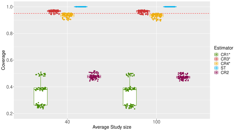
Figure 1: Coverage of the confidence set (9) based on an inversion of the adjusted $F$-test for $k=5$ studies.

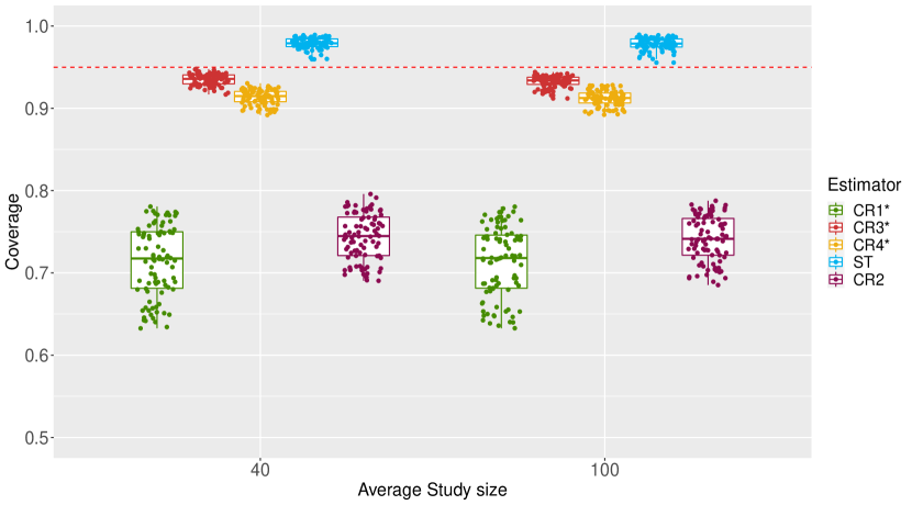
Figure 2: Coverage of the confidence set (9) based on an inversion of the adjusted $F$-test for $k=10$ studies.

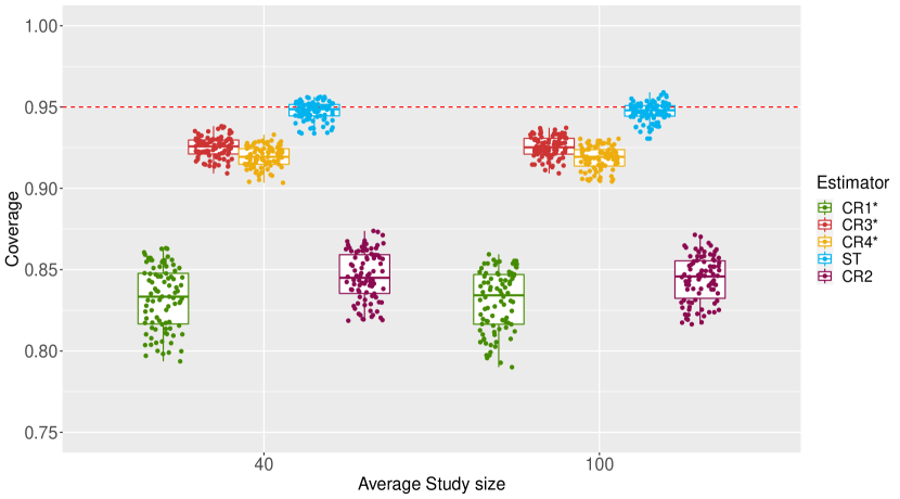
Figure 3: Coverage of the confidence set (9) based on an inversion of the adjusted $F$-test for $k=20$ studies.

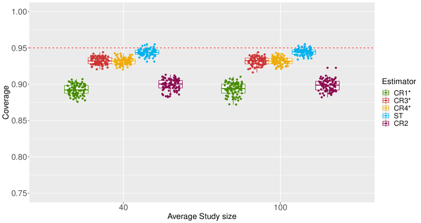
Figure 4: Coverage of the confidence set (9) based on an inversion of the adjusted $F$-test for $k=40$ studies.

In addition to these empirical coverage results, we also consider the power related to the respective tests and confidence regions. The power plots are provided in Figures 5 and 6 for $\boldsymbol{\beta}=(0.2,0.2,0.1,0.1)^{\prime}$ and $\boldsymbol{\beta}=(0.4,0.4,0.2,0.3)^{\prime}$ respectively. We show box plots to summarize the various simulation settings. For $\boldsymbol{\beta}=(0.4,0.4,0.2,0.3)^{\prime}$ power is monotone increasing in the number of studies $k$ for all estimators. For $\boldsymbol{\beta}=(0.2,0.2,0.1,0.1)^{\prime}$ power is monotone increasing in $k$ for $CR_{3}^{*},CR_{4}^{*}$ and $ST$, whereas for $CR_{1}^{*}$ and $CR_{2}$ power decreases from a median of approximately 70% and 60% to 55% and 52% respectively, when going from five to ten studies and then increases in $k$ beyond this point.

The differences in power between the considered estimators are small for a large number of studies and become more pronounced as the number of studies decreases. For forty studies the power based on all estimators is nearly identical for both choices of $\boldsymbol{\beta}$. For twenty studies power based on $CR_{1}^{*}$ and $CR_{2}$ is slightly higher than for the other estimators. $CR_{3}^{*}$, $CR_{4}^{*}$ and $ST$ yield approximately the same power for both choices of $\boldsymbol{\beta}$ and twenty studies. For $k=10$ and $\boldsymbol{\beta}=(0.2,0.2,0.1,0.1)^{\prime}$ the median power for $CR_{1}^{*}$ and $CR_{2}$ is around 55% and 52% respectively, whereas for $CR_{3}^{*}$, $CR_{4}^{*}$ and $ST$ it is around 25%, 31% and 20% respectively. For $k=10$ and $\boldsymbol{\beta}=(0.4,0.4,0.2,0.3)^{\prime}$ the median power for $CR_{1}^{*}$ and $CR_{2}$ is around 87%, whereas for $CR_{3}^{*}$, $CR_{4}^{*}$ and $ST$ it is around 70%, 74% and 73% respectively. For $k=5$ and $\boldsymbol{\beta}=(0.2,0.2,0.1,0.1)^{\prime}$ the median power for $CR_{1}^{*}$ and $CR_{2}$ is around 70% and 60% respectively, whereas for $CR_{3}^{*}$, $CR_{4}^{*}$ and $ST$ it is only around 8%, 12% and 0% respectively. For $k=5$ and $\boldsymbol{\beta}=(0.4,0.4,0.2,0.3)^{\prime}$ the median power for $CR_{1}^{*}$ and $CR_{2}$ is around 83% and 70% respectively, whereas for $CR_{3}^{*}$, $CR_{4}^{*}$ and $ST$ it is around 13%, 24% and 1% respectively.

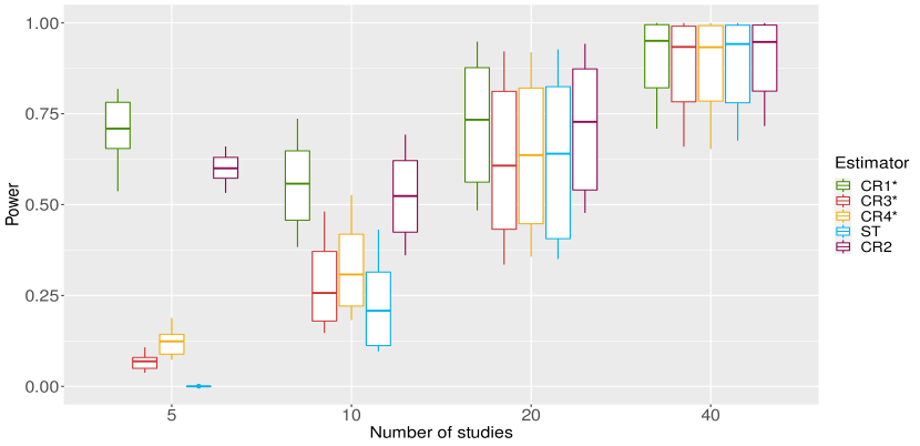
Figure 5: Box plots of power based on adjusted $F$-test for all settings with $\boldsymbol{\beta}=(0.2,0.2,0.1,0.1)^{\prime}$.

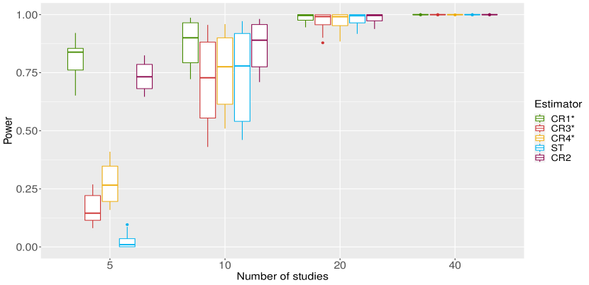
Figure 6: Box plots of power based on adjusted $F$-test for all settings with $\boldsymbol{\beta}=(0.4,0.4,0.2,0.3)^{\prime}$.

6 Discussion

Multivariate Meta-Regression is an important tool for synthesizing and interpreting results from trials reporting multiple, correlated effects. However, information on these correlations is rarely available to analysts, making it difficult to construct the variance-covariance $\boldsymbol{V}$ matrix of the studies’ sampling errors. Cluster-robust estimators allow for a correction of the standard errors, therefore enabling more reliable inference. In this paper we introduced two new proposals of CR estimators for use in multivariate meta-regression. We performed a simulation study, comparing these estimators with results based on two alternative CR estimators and the standard variance-covariance estimator with a focus on coverage and power of confidence sets and tests, as well as an illustrative real life data analysis. In our manuscript we only investigated the bivariate meta-regression setting, although all methods discussed are also applicable in higher dimensions. Further work is necessary to assess the viability of our suggestions in other settings, such as when the number of effects per study is greater than two.

Our main findings can be summarized as follows: The Zhang estimator, discussed in Tipton and Pustejovsky, (2015), can lead to a negative estimate of the denominator degrees of freedom in the $F$-distribution. This can occur when the number of studies is very small. The AHZ approach is therefore not recommendable for bivariate meta-regression if the number of studies is small ($k\leq 5$). Furthermore, when using the classical $F$-test in the bivariate setting, we recommend truncating the denominator degrees of freedom at two. The $CR_{1}^{*}$ and $CR_{2}$ estimators yield an empirical coverage that lies far below the nominal level $1-\alpha$ and the coverage based on the other estimators, especially for smaller numbers of studies. On the flip side the tests based on these two $CR$-estimators unsurprisingly have superior power. The $ST$ estimator has approximately correct coverage for $k\geq 20$ studies but is highly conservative for $k\leq 10$ studies. $CR_{3}^{*}$ and $CR_{4}^{*}$ yield approximately correct coverage for five studies. $CR_{3}^{*}$ also gives nearly correct coverage for ten studies whereas $CR_{4}^{*}$ becomes slightly liberal in this case.

Based on our results we recommend using either the $CR_{3}^{*}$ or $CR_{4}^{*}$ estimator for bivariate meta-regression if $k\leq 10$ with a very slight preference for $CR_{3}^{*}$. For an analysis with $k\geq 20$ studies the $ST$ estimator seems to work best.

A limitation of our simulation study is that the sampling covariances between study-level effects were available for the construction of weight matrices. As mentioned in the introduction, this is often not feasible in practice, requiring analysts to calculate weights using a specified working model for the covariance structure. Hedges et al., (2010) provide possible working models likely to be found in meta-analyses. They propose the use of approximately inverse variance weights, based on these working models.

An open question that requires further research is what the best testing procedure is when the number of studies $k$ is no greater than around five. Neither the adjusted Hotelling’s $T^{2}$ approach in combination with Zhang’s estimator for the degrees of freedom, which was recommended by Tipton and Pustejovsky, (2015), nor the naive or adjusted $F$-tests used in our simulations seem to be the ideal approach. This requires more intensive work that is outside the scope of this manuscript. For a discussion of alternative estimation approaches for the degrees of freedom in the adjusted Hotelling approach, we refer to Tipton and Pustejovsky, (2015). Another question for future research is whether other statistics or resampling approaches that have shown promising small sample approximations for heterogeneous MAN(C)OVA settings (Friedrich et al.,, 2017; Friedrich and Pauly,, 2018; Zimmermann et al.,, 2020) can also help in multivariate meta-regression models.

Data Availability Statement

The neuroblastoma dataset is contained in the R package metafor. All R scripts will be made publicly available, pending publication.

Supplement to “Cluster-Robust Estimators for Bivariate Mixed-Effects Meta-Regression”

Theorem 1.

Suppose there is a $k_{0}\in\mathbb{N}$ such that $k(\boldsymbol{X^{\prime}\widehat{W}X})^{-1}$ exists and is uniformly bounded element-wise for all $k\geq k_{0}$. Furthermore, let $\widehat{\boldsymbol{T}}$ be a consistent estimator for $\boldsymbol{T}$ and $\Lambda$ the confidence region defined in the main paper. Then the $CR$ estimators $CR_{0},CR_{1},CR_{2},CR_{3},CR_{3}^{*},$ $CR_{4}^{*}$ are asymptotically equivalent and we have $P(\Lambda\ni\boldsymbol{\beta})\longrightarrow 1-\alpha$ as $k\rightarrow\infty$.

Proof.

Let $k\in\mathbb{N}$ be the number of studies, $\boldsymbol{\beta}\in\mathbb{R}^{q}$ and $\textbf{X}\in\mathbb{R}^{k\times q}$. Furthermore, $\boldsymbol{\hat{\beta}}=\boldsymbol{(X^{\prime}\widehat{W}X)^{-1}X^{\prime}\widehat{W}y}$ and $\textbf{H}=\boldsymbol{X(X^{\prime}\widehat{W}X)^{-1}X^{\prime}\widehat{W}}$. Then

$$\textbf{H}\boldsymbol{X}=\boldsymbol{X(X^{\prime}\widehat{W}X)^{-1}X^{\prime}\widehat{W}X}=\textbf{X},$$

and since X is a design matrix with the first column equal to $\boldsymbol{1}_{kp}$, all row sums in H are equal to 1. Due to the regularity condition that there exists a $k_{0}\in\mathbb{N}$ such that $\forall\ k\geq k_{0}:\ k(\boldsymbol{X^{\prime}\widehat{W}X})^{-1}$ exists and is uniformly bounded element-wise, we have that for every $i,j\in\{1,\ldots,kp\}:h_{ij}\overset{a.s.}{\rightarrow}0$ as $k\rightarrow\infty$.

So for $i\in\{1,\ldots,k\}$ it holds that $\textbf{H}_{i}\rightarrow\textbf{0}$ as $k\rightarrow\infty$. Here $\textbf{H}_{i}$ refers to the submatrix of H with entries pertaining to study $i$. Thus $(\textbf{I}_{p_{i}}-\textbf{H}_{i})^{\eta}\longrightarrow\textbf{I}_{p_{i}}$ and also $(\textbf{I}_{p_{i}}-\text{diag}(\textbf{H}_{i}))^{\eta}\longrightarrow\textbf{I}_{p_{i}}$ as $k\rightarrow\infty$ for any $\eta\in\mathbb{R}$. It follows that $\boldsymbol{\widehat{\Sigma}}_{a}-\boldsymbol{\widehat{\Sigma}}_{b}\rightarrow\textbf{0}_{q\times q}$ as $k\rightarrow\infty$ for any choice of $a,b\in\{CR_{0},CR_{1}^{*},CR_{3},CR_{3}^{*},CR_{4}^{*}\}$, i.e. they are asymptotically equivalent.

Consider the test statistic

$$Q=\boldsymbol{(\hat{\beta}-\beta_{0})^{\prime}\widehat{\Sigma}^{-1}_{CR}(\hat{\beta}-\beta_{0})},$$

where $\boldsymbol{\widehat{\Sigma}}_{CR}$ is one of the considered $CR$ variance-covariance estimators. Then for any choice of $CR$ estimator (as they are all consistent) we have $\boldsymbol{\widehat{\Sigma}}_{CR}\rightarrow\boldsymbol{\Sigma}=\text{Cov}(\boldsymbol{\widehat{\beta}})$ as $k\rightarrow\infty$. It follows with Slutzky’s Lemma that $Q\overset{d}{\longrightarrow}\chi^{2}_{q}$ as $k\rightarrow\infty$ because with Lemma 2 in White, (1980), it holds that $\boldsymbol{\widehat{\Sigma}^{-1/2}_{CR}\widehat{\beta}}\overset{d}{\longrightarrow}\mathcal{N}(\boldsymbol{\beta},\boldsymbol{I}_{q})$. Furthermore it holds that $qF_{q,k-q,1-\alpha}\overset{d}{\longrightarrow}\chi^{2}_{q,1-\alpha}$ as $k\rightarrow\infty$ because $F_{q,k-q}\overset{d}{=}\frac{\chi_{q}^{2}/q}{\chi_{k-q}^{2}/(k-q)}$, where $\chi^{2}_{q},\chi^{2}_{k-q}$ are independent chi-squared distributed random variables with $q,k-q$ degrees of freedom and $\xi:=\chi^{2}_{k-q}/(k-q)\overset{a.s.}{\rightarrow}1$ as $k\rightarrow\infty$ since $\mathbb{E}(\xi)\equiv 1$ and $\text{Var}(\xi)=\frac{2}{k-q}\rightarrow 0$ for $k\rightarrow\infty$.

Therefore the confidence region $\Lambda$ from the main paper is an asymptotic $1-\alpha$ confidence region for $\boldsymbol{\beta}$.

∎

References

- Bell and McCaffrey, (2002) Bell, R. M. and McCaffrey, D. F. (2002). Bias reduction in standard errors for linear regression with multi-stage samples. Survey Methodology, 28(2):169–182.
- Berkey et al., (1998) Berkey, C., Hoaglin, D., Antczak-Bouckoms, A., Mosteller, F., and Colditz, G. (1998). Meta-analysis of multiple outcomes by regression with random effects. Statistics in Medicine, 17(22):2537–2550.
- Borenstein et al., (2021) Borenstein, M., Hedges, L. V., Higgins, J. P., and Rothstein, H. R. (2021). Introduction to meta-analysis. John Wiley & Sons.
- Cribari-Neto, (2004) Cribari-Neto, F. (2004). Asymptotic inference under heteroskedasticity of unknown form. Computational Statistics & Data Analysis, 45(2):215–233.
- Cribari-Neto et al., (2007) Cribari-Neto, F., Souza, T. C., and Vasconcellos, K. L. (2007). Inference under heteroskedasticity and leveraged data. Communication in Statistics - Theory and Methods, 36(10):1877–1888.
- Davey et al., (2011) Davey, J., Turner, R. M., Clarke, M. J., and Higgins, J. P. (2011). Characteristics of meta-analyses and their component studies in the Cochrane database of systematic reviews: a cross-sectional, descriptive analysis. BMC Medical Research Methodology, 11(1):1–11.
- Friedrich et al., (2017) Friedrich, S., Brunner, E., and Pauly, M. (2017). Permuting longitudinal data in spite of the dependencies. Journal of Multivariate Analysis, 153:255–265.
- Friedrich and Pauly, (2018) Friedrich, S. and Pauly, M. (2018). MATS: Inference for potentially singular and heteroscedastic MANOVA. Journal of Multivariate Analysis, 165:166–179.
- Hayes and Cai, (2007) Hayes, A. F. and Cai, L. (2007). Using heteroskedasticity-consistent standard error estimators in ols regression: An introduction and software implementation. Behavior Research Methods, 39(4):709–722.
- Hedges, (1981) Hedges, L. V. (1981). Distribution theory for Glass’s estimator of effect size and related estimators. Journal of Educational Statistics, 6(2):107–128.
- Hedges et al., (2010) Hedges, L. V., Tipton, E., and Johnson, M. C. (2010). Robust variance estimation in meta-regression with dependent effect size estimates. Research Synthesis Methods, 1(1):39–65.
- Higgins and Thompson, (2002) Higgins, J. P. and Thompson, S. G. (2002). Quantifying heterogeneity in a meta-analysis. Statistics in Medicine, 21(11):1539–1558.
- Jackson et al., (2011) Jackson, D., Riley, R., and White, I. R. (2011). Multivariate meta-analysis: potential and promise. Statistics in Medicine, 30(20):2481–2498.
- Johnson et al., (2014) Johnson, R. A., Wichern, D. W., et al. (2014). Applied multivariate statistical analysis, volume 6. Pearson London, UK:.
- Lin and Aloe, (2021) Lin, L. and Aloe, A. M. (2021). Evaluation of various estimators for standardized mean difference in meta-analysis. Statistics in Medicine, 40(2):403–426.
- Long and Ervin, (2000) Long, J. S. and Ervin, L. H. (2000). Using heteroscedasticity consistent standard errors in the linear regression model. The American Statistician, 54(3):217–224.
- Morris et al., (2019) Morris, T. P., White, I. R., and Crowther, M. J. (2019). Using simulation studies to evaluate statistical methods. Statistics in Medicine, 38(11):2074–2102.
- Olkin and Gleser, (2009) Olkin, I. and Gleser, L. (2009). Stochastically dependent effect sizes. The Handbook of Research Synthesis and Meta-Analysis, pages 357–376.
- Pustejovsky, (2021) Pustejovsky, J. (2021). clubSandwich: Cluster-Robust (Sandwich) Variance Estimators with Small-Sample Corrections. R package version 0.5.3.
- Pustejovsky and Tipton, (2018) Pustejovsky, J. E. and Tipton, E. (2018). Small-sample methods for cluster-robust variance estimation and hypothesis testing in fixed effects models. Journal of Business & Economic Statistics, 36(4):672–683.
- Riley et al., (2007) Riley, R. D., Abrams, K., Lambert, P., Sutton, A., and Thompson, J. (2007). An evaluation of bivariate random-effects meta-analysis for the joint synthesis of two correlated outcomes. Statistics in Medicine, 26(1):78–97.
- Riley et al., (2003) Riley, R. D., Burchill, S., Abrams, K. R., Heney, D., Lambert, P. C., Jones, D. R., Sutton, A. J., Young, B., Wailoo, A. J., and Lewis, I. (2003). A systematic review and evaluation of the use of tumor markers in paediatric oncology: Ewing’s sarcoma and neuroblastoma. Health Technology Assessment.
- Sidik and Jonkman, (2005) Sidik, K. and Jonkman, J. N. (2005). A note on variance estimation in random effects meta-regression. Journal of Biopharmaceutical Statistics, 15(5):823–838.
- Tipton, (2015) Tipton, E. (2015). Small sample adjustments for robust variance estimation with meta-regression. Psychological Methods, 20(3):375.
- Tipton and Pustejovsky, (2015) Tipton, E. and Pustejovsky, J. E. (2015). Small-sample adjustments for tests of moderators and model fit using robust variance estimation in meta-regression. Journal of Educational and Behavioral Statistics, 40(6):604–634.
- Viechtbauer, (2010) Viechtbauer, W. (2010). Conducting meta-analyses in R with the metafor package. Journal of Statistical Software, 36(3):1–48.
- Viechtbauer et al., (2015) Viechtbauer, W., López-López, J. A., Sánchez-Meca, J., and Marín-Martínez, F. (2015). A comparison of procedures to test for moderators in mixed-effects meta-regression models. Psychological Methods, 20(3):360–374.
- Welz and Pauly, (2020) Welz, T. and Pauly, M. (2020). A simulation study to compare robust tests for linear mixed-effects meta-regression. Research Synthesis Methods, 11(3):331–342.
- White, (1980) White, H. (1980). A heteroskedasticity-consistent covariance matrix estimator and a direct test for heteroskedasticity. Econometrica, 48(4):817–838.
- Wilson, (2010) Wilson, J. (2010). Volume of n-dimensional ellipsoid. Sciencia Acta Xaveriana, 1(1):101–6.
- Zhang, (2012) Zhang, J.-T. (2012). An approximate Hotelling T2-test for heteroscedastic one-way MANOVA. Open Journal of Statistics, 2(1):1–11.
- Zimmermann et al., (2019) Zimmermann, G., Pauly, M., and Bathke, A. C. (2019). Small-sample performance and underlying assumptions of a bootstrap-based inference method for a general analysis of covariance model with possibly heteroskedastic and nonnormal errors. Statistical Methods in Medical Research, 28(12):3808–3821.
- Zimmermann et al., (2020) Zimmermann, G., Pauly, M., and Bathke, A. C. (2020). Multivariate analysis of covariance with potentially singular covariance matrices and non-normal responses. Journal of Multivariate Analysis, 177:104594.
Acknowledgements
This work was supported by the German Research Foundation (DFG) (Grant no. PA-2409 7-1). The authors gratefully acknowledge the computing time provided on the Linux HPC cluster at TU Dortmund University (LiDO3), partially funded in the course of the Large-Scale Equipment Initiative by the German Research Foundation as project 271512359.
We would also like to thank James Pustejowsky for his helpful comments during the research phase for this manuscript.