A Variational Quantum Algorithm For Approximating Convex Roofs
George Androulakis and Ryan McGaha
Department of Mathematics, University of South Carolina, 1523 Greene St, Columbia, SC 29208, USA
giorgis@math.sc.edurmcgaha@email.sc.edu
Abstract.
Many entanglement measures are first defined for pure states of a bipartite Hilbert space, and then extended to mixed states via the convex roof extension.
In this article we alter the convex roof extension of an entanglement measure, to produce a sequence of extensions
that we call - extensions, for , where is a fixed continuous function which vanishes only at zero.
We prove that for any such function ,
and any continuous, faithful, non-negative function, (such as an entanglement measure), on the set of pure states of a finite dimensional bipartite Hilbert space, the collection of
- extensions of detects entanglement, i.e. a mixed state on a finite dimensional bipartite Hilbert space is separable,
if and only if
there exists such that the - extension of applied to is equal to zero.
We introduce a quantum variational algorithm which aims to approximate the - extensions of entanglement measures
defined on pure states. However, the algorithm does have its drawbacks. We show that this algorithm exhibits barren plateaus when
used to approximate the family of - extensions of the Tsallis entanglement entropy for a certain function and unitary ansatz of sufficient depth. In practice, if additional information about the state is known, then one needs to avoid using the suggested
ansatz for long depth of circuits.
The work presented here is part of the Ph.D. thesis of the second author which is conducted under
the supervision of the first author for the applied mathematics doctoral program at the University of
South Carolina. As such, results herein may reappear in the PhD dissertation of the second author.
1. Introduction
The detection and quantification of quantum entanglement is a fundamental problem in quantum information theory. A common method for such a quantification is via the use of entanglement measures and entanglement monotones [1, 2, 3, 4]. However, entanglement measures are often difficult to compute for arbitrary density operators, as many of these measures are defined via the convex roof construction. There are some classical numerical algorithms [5] for computing the convex roof of entanglement measures, and even some quantum variational algorithms [6] for computing the logarithmic negativity of arbitrary densities. In this article
we define a family of extensions of entanglement measures defined on pure states, and we introduce a quantum variational algorithm
which aims to approximate these extensions. We prove that the family of certain extensions of the Tsallis entanglement entropy
exhibits barrens plateaus.
First, let us review the definitions of entanglement measures and the convex roof construction in general.
All Hilbert spaces that we consider throughout this article are finite dimensional. Also, if is a Hilbert space
then will denote the set of all density operators on , (i.e. positive semidefinite operators, of trace equal to ).
Definition 1.1.
Let be a finite dimensional bipartite Hilbert space, i.e. for some finite dimensional Hilbert spaces and . Then a function is called an entanglement measure if the following three properties hold for all :
(1)
if and only if is separable, (i.e. is faithful).
(2)
If is a channel of Local Operations and Classical Communications,
(LOCC channel in short), , and is a channel for some convex coefficients and some states , then
. While the structure of LOCC channels is complicated in general, a thorough overview
of LOCC channels can be found in [7]. This property is referred as “LOCC monotonicity” or
“decrease on average under an LOCC channel”).
(3)
where and are unitaries on
and respectively, (i.e. is invariant under local unitaries).
If is defined only on the set of pure states of and satisfies the above properties - for all pure states
of , then we say that is an entanglement measure on the set of pure states of . If is defined only
on the set of pure states of and satisfies the above property for all pure states of , then we say that
is a faithful non-negative function on the set of pure states.
If is a bipartite Hilbert space and is an entanglement measure on the pure states of , then
one extends the domain of to the set of density operators on ,
using the convex roof extension which is defined by
(1)
where is the set of all convex decompositions of with respect to pure states,
often called pure state ensembles. More precisely, is defined by
(2)
It can be shown that the function given by Equation (1) is the largest convex function defined on the
set of all states of , which is less than
or equal to the function on the set of pure states of .
While at first glance it’s not clear that the infimum in Equation (1) is attained, it has indeed been proven
[8, 9] that the infimum is attained as long as the measure is norm continuous on the set of unit vectors of ,
(i.e. on the set of pure states of ).
Terminology 1.2.
The elements of
at which the infimum is achieved are called optimal pure state ensembles or simply OPSEs.
Probably the most prevalent example of an entanglement measure formed in this way is the entanglement of formation, which is first defined on pure states by
(3)
This definition is then extended to the set of all density operators by the convex roof extension method described in
Equation (1). It has been proven that the entanglement entropy is norm continuous on [10], and so the infimum, (OPSE), is always achieved in this case.
Another example of entanglement measurement formed in the same way is the Tsallis entanglement entropy , which is defined by
(4)
for all pure states . It is then extended to general mixed states of via the convex roof construction given in Equation (1), namely
(5)
The natural question that arises is how to find the optimal pure state ensembles that yield the infimum of the
extension of an entanglement measure which is defined on the pure state of a bipartite Hilbert space and is extended to
the mixed states using the convex roof extension. This is an important question because
once the OPSEs are known, then one can compute precisely the entanglement measure.
In this article we give a variational algorithm which aims at approximating the OPSE. It is well known that a main difficulty
in the convergence of variational optimization methods is the existence of Barren Plateaus [11, 12, 13, 14].
Unfortunately, even for
“simple” entanglement measures, such as the Tsallis entanglement measure, to determine whether or not a variational algorithm
has barren plateaus, is not an easy task.
In this article we study barren plateaus of a
variant of the convex roof extension method of the Tsallis entanglement
entropy,
instead of
studying barren plateaus of the Tsallis entanglement entropy itself, since the latter is significantly more technical.
Nevertheless in Section 4 we indicate how one can use the ideas presented here in order to examine barren plateaus of the Tsallis entanglement entropy. Additionally, we believe that our method adapted for the Tsallis entanglement entropy will only predict barren plateaus under
stronger assumptions on the depth of the ansatz than the depth assumptions used in this article. In practice, one will have to avoid using the ansatz
that we use this article for circuits of large depth. This can be possible
if additional information is known about the state whose entanglement is studied.
The variant of the convex roof extension method that we use here
does not yield an entanglement measure, but it is still allows us to detect
entanglement. It depends on a fixed function which vanishes only at zero,
and it yields a family of extensions indexed by the integers . The domains of these extensions increase with ,
and they become equal to the set of density operators on the Hilbert space when is large enough, (more precisely, when
strictly exceeds the dimension of the manifold of the density operators on the given bipartite Hilbert space).
These extensions decrease with respect to at any fixed density operator, and their infimum for all is equal to zero.
More precisely, we have the following definition.
Definition 1.3.
Let be a bipartite Hilbert space, be an entanglement measure on the set of pure states of , and
be a function that vanishes only at .
For every define the set of density operators of that can be written as a convex combination of at most
many pure states, i.e.
(6)
Note that
(i)
is equal to the set of pure states of , (in this case, ).
(ii)
for every , (since the ’s are allowed to be equal to zero).
(iii)
There exists such that , (indeed, by Caratheodory’s theorem in convex analysis, this happens when ).
Define a function by
We call the function the “- extension of ”. We call the sequence
the “sequence of -extensions of ”.
Remark 1.4.
Let be a finite dimensional bipartite Hilbert space, be a continuous, non-negative function on the set of pure states of ,
and
be a continuous function which vanishes only at . Then, for every the infimum in the
definition of is attained, (i.e. it is a minimum).
Indeed, since is finite dimensional, the set of pure states on is a compact set. Let denote the set
of pure states on . Also, the set
is compact as well. Now the function defined on by
is a continuous function, since both and are assumed to be continuous. Hence it achieves its minimum on its compact domain,
which finishes the proof of Remark 1.4.
Let be a finite dimensional bipartite Hilbert space, be a continuous non-negative function on the set of pure states of ,
and be a continuous function which vanishes only at . Let , and .
The tuple
with for all , ,
being pure states on , and ,
is called “Optimal Pure State Ensemble (OPSE) for , and ”.
In this article we study the sequence of -extensions of Tsallis
entanglement entropy , where is defined by .
We will denote by the sequence of -extensions of Tsallis entanglement entropy defined on the set of
pure states of a bipartite Hilbert space . More precisely, by combining Equation (4) and
Definition 1.3 we obtain
(7)
Remark 1.6.
The reason that we bound the length of the convex combinations in Definition 1.3 by a finite number ,
is because otherwise the infimum in Equation (7) would be equal to zero for every .
Indeed, in order to verify the statement of Remark 1.6, notice that if
for some
with and a sequence of pure states ,
then for every
we can write (i.e. we divide each by and we repeat times), and
which tends to zero as tends to infinity.
Given an entanglement measure on the set of pure states of a finite dimensional bipartite Hilbert space,
and a continuous function which vanishes only at , the
sequence of the -extensions of can be used in order to detect entanglement in the following sense:
Definition 1.7.
Let be a bipartite Hilbert space, and for every let be a subset of the set of density
matrices of , satisfying properties , and of Definition 1.3.
For every let a function . We say that the family
detects entanglement, if for every density operator on ,
is separable if and only if there exists such that and .
Proposition 1.8.
Let be any continuous, faithful, non-negative function on the set of pure states of a finite dimensional bipartite Hilbert space
. Let be a continuous function that vanishes only at zero.
Then, the - extensions of to the density operators of , detect entanglement, as in the previous definition.
Proof.
Let be a mixed state on such that for some . Then by Remark 1.4, there exists some pure state ensemble with and
(8)
If we assume without loss of generality that each , then it must follow that
for each . Since is a faithful, non-negative function on the set of pure states,
it must be true that is factorable for each . Thus can be written as a convex combination of factorable pure states, and is therefore separable.
Conversely, suppose that is separable. Then there exists some ensemble , of such that each is factorable.
Therefore for each and so
(9)
∎
2. The Algorithm
It is difficult to compute optimal pure state ensebles in Equation (1) or in Terminology 1.5, because the proof
for their existence, (given in Remark 1.4), is not constructive. However, methods for approximating them on a quantum computer are heavily implied by the following theorem [15, 16, 17, 18, 19].
Theorem 2.1(Purification Theorem).
Let be a finite dimensional Hilbert space and suppose that can be expressed as both of the following pure state ensembles:
and define
(10)
where is an orthonormal basis for . Then there exists a unitary such that .
This theorem tells us that any two pure state ensembles of the same length are related by a unitary map.
So if we already know one pure state ensemble of a given density, we can find all others simply by applying unitaries
on the ancilla space of a purification of . Hence we can minimize the quantity
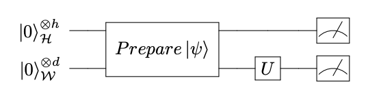
over the unitary group, where the and are as in the previous theorem, and is an arbitrary entanglement measure. Moreover, the theorem hints at using the following quantum circuit to achieve our goal.
Figure 1. The quantum circuit implied by the purification theorem.
Here and , while where is the ancilla space. In particular, is also the length of the pure state decompositions output from the circuit. Usually is taken to be greater than .
Examining the circuit, notice that after preparing the system in the state and applying the unitary , the system
is put into the superposition . When measuring the system, if the state
is observed on the ancilla space, then it must be the case that the top qubits are in the state
with certainty. Running this circuit a number of times allows the observer to experimentally reconstruct both and , and therefore compute the quantity . In order to find the optimal pure state ensemble we need
expressions for and in terms of .
By examining the circuit step by step, we see that the circuit first prepares the purification . The unitary is then
applied to the ancilla space resulting in the state . Lastly, measuring
the ancilla yields the states
(11)
where
(12)
And to access the state on the space , we partial trace the ancilla and use the partial cyclicity of the partial trace to arrive at the following expression for the states
(13)
for each in .
Convention 2.2.
Since all of the sums that follow range from 1 to , we will often write to mean .
The natural question that arises is how to search the unitary group for the unitary that minimizes the quantity where the and as in Equations (12) and (13) respectively, and is an entanglement measure or related function. There are several ways to accomplish this task, the most common being the utilization of a parametrization of the unitary group [20] and applying geometric optimization techniques as in [5], or the use of random parametrized quantum circuits [21, 22, 23, 6]. We choose the latter, as this choice will greatly simplify calculations in the proof of our main result. Specifically, we will use parametrized unitaries of the following form:
(14)
where is a Hermitian operator, for each , and is an entangling gate
independent of the parameters . Common choices for are a or ladder. In applications,
the operators are often taken to be a randomly chosen string of Pauli operators, which is the convention that we use. Indeed, it is well known that the gates , , , the phase gate and form a universal gate set, (see [24, Section 2.6]).
Since we have introduced the parameters into our unitaries, the ansatz we wish to train can be written
as , thus allowing us to use common
optimization techniques to approximate the minimum. Thus a quantum algorithm to approximate optimal pure state ensembles can be
summarized as below:
Input: An ensemble of a density matrix ,
and an optimization routine, (as in [25]).
Parameters: Initial parameters .
whileOptimization routine has not convergeddo
Prepare the purification on .
Construct as above and apply to the ancilla, .
Measure.
Use measurements to compute (or related quantities such as gradients as required by the chosen optimization technique).
Update according to optimization routine.
return .
Algorithm 1Variational Approximation of OPSE
An algorithm of this type is called a variational quantum algorithm(VQA) [26]. VQA has shown great success in various settings such as Hamiltonian Simulation and Quantum Machine Learning [21, 26, 27, 28] where most cost functions are physically implementable on a quantum computer. In the algorithm described above, we instead train a nonlinear cost function on the measurements of a physically implementable ansatz. While VQA is believed, (not yet proven), to offer a possible quantum advantage over classical algorithms for certain problems [26, Chapter 1 - Section C], there are still drawbacks, namely the issue of Barren Plateaus [11, 12, 13, 14]. These are regions of the training landscape on which the partial derivatives with respect to the parameters decrease exponentially as the number of qubits in the experiment increase. More precisely, we give the following definition.
Consider the ansatz in Equation (14) on qubits where , with objective function
(15)
Then the training landscape will contain barren plateaus in the parameter for some , if
(16)
where the variance is taken with respect to the Haar measure on the Unitary group, is the number of qubits, and
is a real number [13]. When this variance is exponentially small, the ansatz can become untrainable in practice because an exponentially large amount of precision will be required on the classical hardware to evaluate the derivatives. For instance, if it were shown that the variance is on the order of , where is the number of qubits, then systems with only 100 qubits can start creating difficulties since the number of classical bits required to differentiate the values of the gradient from 0 will be in the order of .
In this article we show that the --extension
of the Tsallis entanglement entropy for exhibits
barren plateaus when using the ansatz given in Equation (14)
of large depth, (thus in particular, if no additional information is
available about the state whose entanglement is examined). In practice, if additional information about the state is known, then one needs to avoid using the suggested
ansatz for long depth of circuits. Recall that
is given by Equation (7).
While the OPSE of will yield if we allow infinitely long decompositions as considered in
Remark 1.6, is still useful in
determining whether a state is entangled, as long as we consider decompositions of finite length, (by Proposition 1.8).
Also, obviously, is local unitary invariant (just as the Tsallis
entanglement entropy ), but is not LOCC monotonic.
In order to set the ground for Theorem 2.3, first
define the cost function for the algorithm, that needs to be minimized, to be equal to
which is given by
(17)
To simplify notation somewhat, we define by
(18)
For readability, we will usually suppress the parameters
and simply write .
Since, by Equation (4), can be equivalently rewritten
from Equation (7) to
(19)
we can write succinctly as
(20)
Notice that the last quantity is non-negative, since
for all positive operators . Indeed, let be the spectral decomposition of . Then all eigenvalues are non-negative and the are mutually orthogonal projections with for each . Thus
(21)
We show some modest limits on the trainability of as summarized by the following theorem.
Theorem 2.3.
If the parametrized circuit in Equation (14) is of sufficient depth, then for each , , where the objective function is defined in Equation (7), the variance is taken with respect to the Haar measure on the unitary group, and is the number of qubits.
Because of the length of the proof of the above theorem, its proof is presented in the appendix of this article.
Remark 2.4.
As shown in the proof of Theorem 2.3, the circuit must have a relatively large depth in order for a barren plateau to occur. Thus for most practical purposes, the ansatz should still be trainable since less expressive circuits are often used in practice. It is also possible to construct more “friendly”ansätze by taking into consideration properties of the given density matrix such as translation invariance.
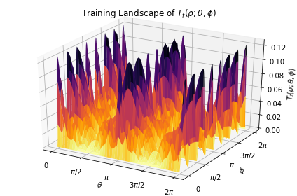
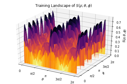
Figure 2. Training landscape of where is the maximally mixed state and .
3. Numerical Simulations
Recall that for a two qubit state , the concurrence [1, 29] is defined by
(22)
The concurrence is related to the von Neumann entanglement entropy via the formula
(23)
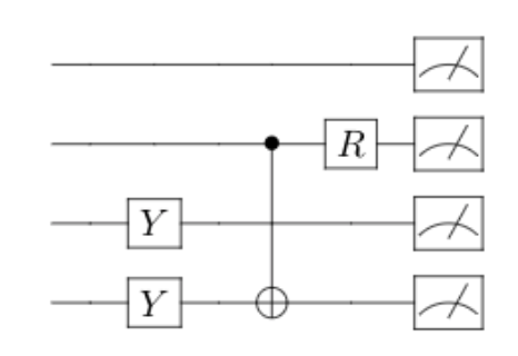
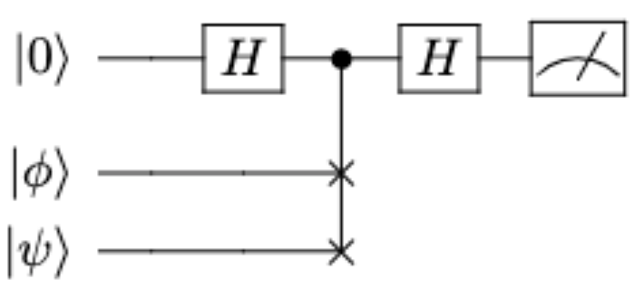
where is the standard binary entropy defined by [1]. Interestingly enough, it is possible to directly measure the concurrence of a 2 qubit quantum system if there is access to two decoupled copies of the same state [29]. One can do this using the quantum circuit in Figure 3, where the first two wires as well as the last two wires are in the state respectively, and is the unitary
(24)
Figure 3. Quantum circuit for directly measuring concurrence in 2 qubit states.
After applying these operations to the state , the probability amplitude of the state will be .
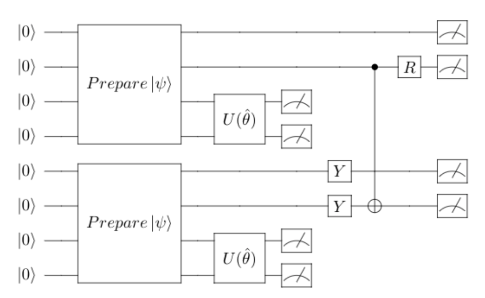
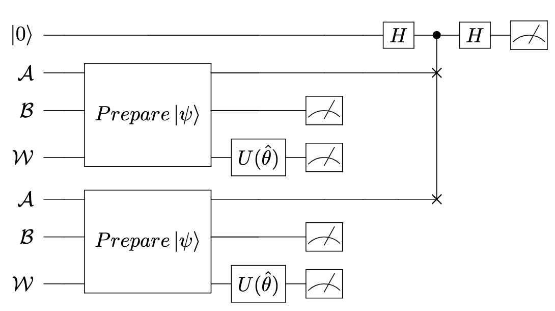
Using the above ideas, we can append the circuit for measuring the concurrence of a state to the pure state ensemble circuit, so that we can measure the concurrence of a 2 qubit ensemble of states directly, and therefore efficiently compute the entanglement of formation for 2 qubit states. The entire circuit for this process is given in Figure 4 for an arbitrary density matrix with a purification requiring two qubits.
Figure 4. Quantum circuit for variationally approximating the entanglement of formation by directly measuring the concurrence of pure state ensembles.
Let’s go through the circuit in Figure 4 step by step since there’s a lot going on. We first prepare the purification of a two qubit density operator on the first four and last four quantum registers so that we can access two decoupled copies of the pure state ensemble. Next we apply to both of the ancilla spaces and measure the ancillae. This will put the top two registers into the state , (as in Equation (13)), the third and fourth registers into the state , the 5th and 6th registers into the state , (again, as in Equation (13)), and the last two registers into the state , where . Thus the state of circuit at this point is then . If , then we can measure the concurrence by appending the circuit in Figure 3 to wires 1,2,5, and 6, and taking note of the frequency of the state where the first two registers are in state , the third and fourth are in state , the fifth and sixth are in state , and lastly the 7th and 8th are in the state . We then run this experiment a desired number of times to also make note of the probabilities as defined as in Equation (12) and the concurrence for each . Lastly we use the measurements to approximate the entanglement entropy in the equation below via
(25)
Using the maximally mixed state and its canonical purification with 4 ancillae, we simulated the above variational algorithm and showcase our results in Figures 5 and 6.
Figure 5. The training landscape of where is the maximally mixed state and .Figure 6. Convergence of the algorithm for the entanglement of formation of the maximally mixed state.
The python code corresponding to the simulations and plots can be found at https://github.com/TheMathDoctor/code_for_vqa_paper. These simulations made extensive use of both the numpy [30] and matplotplib [31] python libraries.
4. Approximating the Tsallis Entanglement Entropy Via The Swap Test
In this section we discuss some additional applications of the algorithm discussed in Section 2. Specifically, we show that it is possible to measure the convex roof extended Tsallis entanglement entropy directly using the swap test [32].
Recall that the swap test can be used to estimate the quantity with error using the circuit in Figure 7 using quantum queries. When running this circuit a large number of times, an observer will measure on the top wire with probability , and an observer will measure on the top wire with probability .
Figure 7. Quantum circuit used for the swap test.
To see how this is useful for computing the Tsallis entropy of a state, consider a density operator where and the are pure states which are not necessarily orthonormal.
Then . Thus, in order to compute the Tsallis entropy of which is given by , (not to be confused with the Tsallis entanglement entropy of a pure bipartite
state given in Equation (4)),
one needs to run the circuit in Figure 7 with inputs and for each and , measure the probability of measuring for each combination, and then weight the outputs by the appropriate probabilities . In summary, if approximate values of ’s can be computed,
then the Tsallis entropy of can be approximated via
(26)
Now we need to see how circuit is useful for approximating the Tsallis entanglement entropy, let
and let be a purification of as in Equation (10). Next
let and be as in Equations (13) and (12). Then, the Tsallis
entanglement entropy of can be approximated by minimizing the expression
(27)
with respect to the and . However, the swap test requires two copies of the state, so we need to have two adjacent copies the pure state ensemble circuit, each of them as in Figure 1, in order to access two copies the various ensembles of and then append the quantum circuit for the swap
test. Thus we need a quantum circuit very similar to the circuit in Figure 4. The full circuit
for this process is given in figure 8.
Figure 8. Quantum circuit for approximating Tsallis Entanglement Entropy
Let’s go through this circuit one operation at a time to understand what’s going on, so that we can point out some loose
quantum query complexity constraints on this process. Before we begin, notice that in this circuit, we specified wires for the Hilbert spaces and instead of specifying one wire for . The reason for this is that we need to partial trace (measure and discard) either the or subsystems in order to approximate the Tsallis entanglement entropy.
First, we need to prepare two decoupled copies of the purification of a given density and apply
to each ancilla . Then we measure each ancilla . If we obtain measurements
and on the two ancillas, then the state of the circuit will collapse into
, (where is on the top wire, and
and are on the wires representing the two copies of ).
If , then all other operations will produce no useful information and we just use the observations to
approximate and .
Otherwise, if , then the state of the circuit will be
. In this case, we measure the space with respect
to a fixed basis (say the standard -basis) and collect all measurements weighted according to their probabilities
into one density matrix on the space .
The density matrix that is obtained that way is equal to
for some probabilities
and some pure states on for each .
Therefore, upon measuring and discarding the wire(s) for the space , the first wire for will be in the state
, and the second wire for will be the state for some and
each appearing with probabilities and respectively.
Then, the swap test circuit given in Figure 7 is appended with inputs and
. As we noticed earlier, we will measure on the top wire with probability
.
Moreover, the state will occur with frequency where is the number of shots. One can then run this experiment a desired number of times in order approximate which can seen to be equal to
(28)
for each . Thus, the Tsallis entanglement entropy of is approximated by
(29)
Next we need to think about the algorithmic complexity of this approximation. In order for the quantum circuit to yield useful information both
ancillae must be in the same state for some . By equation (12), this happens with probability . Thus if we consider
the Bernoulli random variable such that “i=j”occurs with probability and “ij”occurs with
probability , then the expected number shots until the first success is given by . Since
for each , we can see that the average number of shots until the first success,
i.e. , is then greater than or equal to by applying Jensen’s inequality
using the convex function for .
And since where is the number of qubits in the system, we can see that the approximation will require exponentially many shots on average in order to compute within
some error for a fixed . Thus, while we are able to approximate the Tsallis entanglement entropy directly via the measurements of a quantum circuit, the process is inefficient.
While we do not prove it here, we suspect that there should be similar results for the von Neumann entanglement entropy
and related quantities using methods found in [33, 34]. We also leave as an open to problem to determine
if this objective function suffers from barren plateaus.
5. Concluding Remarks
We have shown how to access the different pure state ensembles of a given density operator using a quantum computer. We are thus able to approximate entanglement measures and related quantities that use convex roof constructions using a variational method and measurements from a parametrized quantum circuit. However we also show that the training landscape of a quantity related to the Tsallis entanglement entropy exhibits barren plateaus for a certain ansatz
and for circuits of large depth, effectively making the ansatz untrainable for large enough systems. In practice, if additional information about the state is known, then one needs to avoid using the suggested
ansatz for long depth of circuits. Lastly, we leave as an open problem the determination of barren plateaus of other entanglement measures and related quantities.
References
[1]
R. Horodecki, P. Horodecki, M. Horodecki, and K. Horodecki.
Quantum entanglement.
Rev.Mod.Phys., 81:865–942, 2009.
[2]
M. B. Plenio and S. Virmani.
An introduction to entanglement measures.
Quant. Inf. Comput., 7:1–51, 2007.
[3]
V. Vedral, M. B. Plenio, M. A. Rippin, and P. L. Knight.
Quantifying entanglement.
Phys.Rev.Lett., 78:2275–2279, 1997.
[4]
G. Vidal.
Entanglement monotones.
J.Mod.Opt., 47:355–376, 2000.
[5]
B. Röthlisberger, J. Lehmann, and D. Loss.
Numerical evaluation of convex-roof entanglement measures with
applications to spin rings.
Phys. Rev. A, 80, 2009.
[6]
K. Wang, Z. Song, X. Zhao, Z. Wang, and X. Wang.
Detecting and quantifying entanglement on near-term quantum devices,
2020.
[7]
E. Chitambar, D. Leung, L. Mancinska, M. Ozols, and A. Winter.
Everything you always wanted to know about locc (but were afraid to
ask).
Comm. Math. Phys., 328:303–326, 2014.
[8]
M. Shirokov.
On properties of the space of quantum states and their application to
the construction of entanglement monotones.
Izvestiya: Math., 2:849–882, 2010.
[9]
G. Androulakis and R. McGaha.
Some remarks on the entanglement number.
Quanta, 9:22–36, 2020.
[10]
M. Fannes.
A continuity property of the entropy density for spin lattice
systems.
Comm. Math. Phys., 31:291–294, 1973.
[11]
J. McClean, S. Boixo, V.. Smelyanskiy, R. Babbush, and H. Neven.
Barren plateaus in quantum neural network training landscapes.
Nature Communications, 9, 2018.
[12]
M. Cerezo, A. Sone, T. Volkoff, L. Cincio, and P. Coles.
Cost function dependent barren plateaus in shallow parametrized
quantum circuits.
Nature Communications, 12, 2021.
[13]
A. Arrasmith, Z. Holmes, M. Cerezo, and P. Coles.
Equivalence of quantum barren plateaus to cost concentration and
narrow gorges, 2021.
[14]
A. Pesah, M. Cerezo, S. Wang, T. Volkoff, A. Sornborger, and P. Coles.
Absence of barren plateaus in quantum convolutional neural networks.
Physical Review X, 11, 2021.
[15]
E. Schrödinger.
Probability relations between separated systems.
Proceedings of the Cambridge Philosophical Society,
32:446–452, 1936.
[16]
L. Houghston, R. Josza, and W. Wooters.
A complete classification of quantum ensembles having a given density
matrix.
Physical Letters A, 483:14–18, 1993.
[17]
N. Hadjisavvas.
Properties of mixtures on non-orthogonal states.
Letters in Mathematical Physics, 5:327–332, 1981.
[18]
N. Merman.
What do these correlations know about reality? nonlocality and the
absurd.
Foundations of Physics, 29:571–587, 1999.
[19]
N. Gisin.
Stochastic quantum dynamics and relativity.
Helvetica Physica Acta, 62:363–371, 1989.
[20]
C. Spengler, M. Huber, and B. Hiesmayr.
A composite parameterization of unitary groups, density matrices and
subspaces.
Journal of Physics A: Mathematical and Theoretical, 43, 2010.
[21]
A. Kandala, A. Mezzacapo, K. Temme, M. Takita, M. Brink, J. Chow, and
J. Gambetta.
Hardware-efficient variational quantum eigensolver for small
molecules and quantum magnets.
Nature, 548:242–246, 2017.
[22]
J. Romero, R. Babbush, J. McClean, C. Hempel, P. Love, and A. Aspuru-Guzik.
Strategies for quantum computing molecular energies using the unitary
coupled cluster ansatz.
Quantum Science and Technology, 4, 2018.
[23]
J. McClean, S. Boixo, V. Smelyanskiy, R. Babbush, and H. Neven.
Barren plateaus in quantum neural network training landscapes.
Nature Communications, 9, 2018.
[24]
Collin P. Williams.
Explorations in Quantum Computing.
Springer London, 2011.
[25]
W. Press, S. Teukolsky, W. Vetterling, and B. Flannery.
Numerical Recipes: The Art of Scientific Computing.
Cambridge University Press, 2007.
[26]
K. Bharti, A. Cervera-Lierta, T. H. Kyaw, T. Haug, S. Alperin-Lea, A. Anand,
M. Degroote, H. Heimonen, J. Kottmann, T. Menke, W. Mok, S. Sim, L. Kwek, and
A. Aspuru-Guzik.
Noisy intermediate-scale quantum (nisq) algorithms.
Reviews of Moder Physics, 94, 2022.
[27]
M. Cerezo, A. Arrasmith, R. Babbush, S. Benjamin, S. Endo, K. Fujii,
J. McClean, K. Mitarai, X. Yuan, L. Cincio, and P. Coles.
Variational quantum algorithms.
Nature Reviews Physics, 3(9):625–644, Aug 2021.
[28]
J. Lau, K. Bharti, T. Haug, and L. Kwek.
Noisy intermediate scale quantum simulation of time dependent
hamiltonians, 2021.
[29]
G. Romero, C. López, F. Lastra, E solano, and J.C. Retamal.
Direct measurement of concurrence for atomic two-qubit pure states.
Physical Review A, 75, 2007.
[30]
C. Harris, K. Millman, S. van der Walt, R. Gommers, P. Virtanen, D. Cournapeau,
E. Wieser, J. Taylor, S. Berg, N. Smith, R. Kern, M. Picus, S. Hoyer, M. van
Kerkwijk, M. Brett, A. Haldane, J. Fernández del Río, M. Wiebe,
P. Peterson, P. Gérard-Marchant, K. Sheppard, T. Reddy, W. Weckesser,
H. Abbasi, C. Gohlke, and T. Oliphant.
Array programming with NumPy.
Nature, 585(7825):357–362, September 2020.
[31]
J. Hunter.
Matplotlib: A 2d graphics environment.
Computing in Science & Engineering, 9(3):90–95, 2007.
[32]
Harry Buhrman, Richard Cleve, John Watrous, and Ronald de Wolf.
Quantum fingerprinting.
Physical Review Letters, 87, 2001.
[33]
Tom Gur, Min-Hsiu Hsieh, and Sathyawageeswar Subramanian.
Sublinear quantum algorithms for estimating von neumann entropy,
2021.
[34]
Qisheng Wang, Ji Guan, Junyi Liu, Zhicheng Zhang, and Mingsheng Ying.
New quantum algorithms for computing quantum entropies and distances,
2022.
[35]
L. Zhang.
Matrix integrals over unitary groups: An application of schur-weyl
duality, 2015.
[36]
B. Collins.
Moments and cumulants of polynomial random variables on unitary
groups, the itzykson-zuber integral, and free probability.
International Mathematics Research Notices, 17:953–982, 2003.
[37]
S. Matsumoto.
Weingarten calculus for matrix ensembles associated with compact
symmetric spaces.
World Scientific, 2, 2013.
[38]
M. Fukuda, R. König, and I. Nechita.
Rtni—a symbolic integrator for haar-random tensor networks.
Journal of Physics A: Mathematical and Theoretical,
52:425–303, 2019.
[39]
M. Fukuda, R. König, and I. Nechita.
Rtni_light_web, 2019.
[40]
A. Harrow and R. Low.
Random quantum circuits are approximate 2-designs.
Communications in Mathematical Physics, 291:257–302, 2009.
[41]
F. Brandão, A. Harrow, and M. Horodecki.
Local random quantum circuits are approximate polynomial-designs.
Communications in Mathematical Physics, 346:397–434, 2016.
Appendix A Integration Over The Unitary Group
In order to prove Theorem 2.3, we’ll need the following results on integrals over the unitary group [35, 36]:
Lemma A.1.
For any strings of indices and whose values range from to
(30)
where is the Haar-Measure on the Unitary group and Wg is the Weingarten function [37, 38].
While notation can make this lemma difficult to parse at first glance, notice that the integral is 0 when the number of complex conjugate entries of the matrix is different the number of non-conjugated entries. Unfortunately, the integrals used in this paper aren’t lucky enough to fall into this category and we must instead use the expression on the right hand side of the equation to evaluate our integrals. Since this expression can be difficult to understand at first, we supply a simple example of computing such an integral via this lemma.
Example A.2.
Let be unitary matrices on . Then the average gate fidelity between and , , is defined by
(31)
where is unit ball of .
Such an integral over pure states is defined by
(32)
where each is replaced by for some arbitrary state . Now let be a basis for and without loss of generality, set . Next write and suppose that has spectral decomposition
(33)
where with for each and is some unitary on . Using these substitutions, the integral in Equation(32) transforms as
(34)
Now using the translation invariance of the Haar measure on , we use a change of variable to simplify the above integral. Set so that . Therefore
(35)
We can now use the integration formula given in (A.1) to evaluate the integral in the last expression of the previous equation and we arrive at
(36)
where and . Since is a unitary, each has absolute value 1, and so
(37)
To compute the other sum, we use the fact that the sum of the eignvalues of a matrix is its trace, so that
(38)
Recalling that , we can see that where the inner product is taken to be the Hilbert-Schmidt inner product.
Thus it follows that
(39)
We can see that in order to compute these integrals, we must be familiar with the Weingarten function on the unitary group. In general, the Weingarten function can be difficult to compute, and we therefore include a table of values for the Weingarten function for the first four permutation groups as we’ll need these values in the computation of the variance of concern. In table (1), we list the cycle structure of a given permutation in the left hand column and the the value of in the right hand column. These values were computed using the tool [39] written by M. Fukuda et alii.
Table 1. Table of Values for the Weingarten function
Cycle Structure of
1
1,1
2
1,1,1
2,1
3
1,1,1,1
2,1,1
2,2
3,1
4
Notice that the value of the Weingarten function of a given permutation is dependent only on the cycle structure of a permutation. For example, let . This permutation has cycle structure 2,2 and so .
Before computing the mean and variance of the derivatives of the cost function , we must first discuss the probability distribution of unitaries produced by the circuits defined in Equation(14).
In order to make the notation more readable, suppose that for some and that . Then the derivative of with respect to can be written as
(40)
The derivative splits the circuit into two “pieces”, the left side and the right side which we define accordingly
(41)
which lets us write . Moreover, using this expression for the derivative of lets us express as
(42)
We will often write for readability so that
(43)
This splitting forces us to consider the distributions of the and separately. Therefore, just as in the paper [23] by McClean et alii, we write the probability distribution generated by the entire circuit as
(44)
where and are the Haar measure on , and are densities on , and is the dirac measure centered at the matrix. This distribution forces any unitary to be split as the product of two other unitaries and with their own distributions and respectively. To quantify these distribution we’ll need to use the notion of unitary k-designs. A distribution is defined to be a k-design if matches the Haar measure on the unitary group up to and including the k-th moment [40, 41, 35, 36]. In other words,
(45)
for all . In practice, exact -designs are costly to produce. And so we’ll also need the notion of an approximate -design [41]. We say that a a measure is an -approximate -design if and only if
(46)
for any , where and is the Haar measure on . Such measures are attainable in practice using only polynomially many gates in the number of qubits [40, 41], thus the result is relevant for NISQ devices.
With the distribution from Equation (44) in mind, we will split the computation of the mean and variance of into two cases; One in which we assume that is a 4-design, and the other in which is a 4-design. Note that this assumption is a practical one since it has been proven [40, 41] that polynomial depth quantum circuits such as those given in Equation (14) are approximate k-designs, if they are of sufficient depth. Therefore, since the gates used the ansatz of
Equation (14) form a universal gate set, if the depth of that
ansatz is sufficiently large, then at least one of and that appear in Equation (41) has sufficient depth in order to yield that or is a 4-design.
Next let’s expand the various components of using the definitions of and , given in Equations (12) and (18) respectively, for each .
(47)
It can be shown in a similar fashion that
(48)
Using the commutator expression given in Equation (42) for the derivative of as follows:
(49)
In the same way, a similar expression is found for :
(50)
Putting all of this together we see that
(51)
Also, has a similar expression:
(52)
which can be seen to be equal to
(53)
Putting all of this together, we can expand as
(54)
and then integrate this expression term by term using the expressions above. In what follows, we’ll fix an and integrate the terms and separately for clarity. After the computation of the integrals, we’ll then sum the results to arrive at the appropriate expected value.
Now notice that the expressions given in equations (51) and (53) are of the form
(55)
where for any choice of indices. Because we only need an upper estimate for our variance, we’ll soon see that we don’t need the exact values of the and that we’ll only use the fact that they are bounded in absolute value by 1. Next we need to integrate the above expression with respect to the distribution . Since only the expression is dependent on and , we can integrate this expression and substitute its value back into Equation (55).
In the integration formula given in Lemma A.1, the expressions that were integrated were given in terms of the coordinates of the unitaries, but the expression we currently have is not in this form. We must therefore force the expression into this form and expand the commutator . It’s easy to see that is, up to a multiple of , equal to
(56)
For our computations, we’ll just use the first term, , of the commutator since the computations with the second term are nearly identical. Suppose for now that is at least a 2-design, then is equal to the Haar-distribution up to the second moment. Thus
(57)
Using the translation invariance of the Haar-integral on the Unitary group, we define the change of variables with . The integral then becomes
(58)
The last thing that we need to do before using the integration formula is to express in terms of the coordinates of . To do this, first define so that
(59)
and thus
(60)
Substituting this expression back into the integral we see that
(61)
Notice that all of the row coordinates of the ’s in the integral are equal to , so we can suppress the terms in the integration formula from Lemma (A.1) since they are always equal to 1. The index also took the place of in the column coordinate of one of the s in the last expression of the above equation.Therefore the must be treated as a when using the integration formula from Lemma A.1. For clarity, we isolate the inner integral and compute it as follows:
(62)
Defining and substituting the last expression of the above equation back into Equation (61), we see that the value of the integral is equal to
(63)
Ignoring the integral and outside constants for the moment, let’s plug the expressions and into Equation (55) and try to bound the sum in absolute value. Substituting , we see that
(64)
Now taking absolute values,
(65)
Lastly using the Cauchy-Schwartz inequality and the fact that the Hilbert-Schmidt norm of a unitary matrix is equal to , we can see that
(66)
The computation when substituting the term is almost exactly the same so we omit it for brevity. We have thus showed that when is at least a 2 design and is an arbitrary distribution, the integral of Equation (55) is bounded in absolute value as
(67)
And since both and are both bounded by the above integral, it follows that
(68)
Therefore
(69)
This shows that the expected gradients converge exponentially to 0 in the number of qubits when is at least a 2-design and the distribution of is arbitrary.
Suppose now that the distribution of is at least a 2-design and the the distribution of is arbitrary. We will make almost the same change of variables as before with and . However we now define so that
(70)
Now using the same steps as in the first case in Equations (59) and (60), we arrive at the integral
(71)
And again we now substitute one of the expressions containing deltas into Equation (55) and bound the expression.
(72)
Since both the and are bounded in absolute value by 1, we see that
(73)
Now we the same steps as in Equations (68) and (69) to compute the expected value again. Thus in the case when is at least a 2-design and is given by an arbitrary distribution, we see that
(74)
We now need to compute the second moment of the . We will accomplish this by squaring the expression in Equation (54) and integrating term by term just as we did with mean. In order to compute these integrals, we need stronger,but still modest, assumptions on the distributions of amd . Namely we must split into cases when is a 4-design and is not, and vice versa. Note that such a circuit is indeed possible in practice and only needs to be of polynomial depth [41].
First let’s square the sum in Equation (54) to understand what we’re working with.
(75)
When multiplying term by term in the last line of the equation above, making substitutions using Equations (47) through (50) and using the same change of variables , we encounter expressions of the form
(76)
for each each fixed and . Just as we did in the computation of the mean, we will fix and , compute the appropriate integrals for each term, and sum the results at the end.
Again, we only need to worry about the terms of the above equation that involve only entries of , , or when integrating, and can substitute the values of these integrals back into the Equation. Because there are now two commutators, and , in the expression, we’ll need to break our proof into cases based on which terms of the commutator are multiplied together. To understand the cases better, let’s expand fully expand . Using the definitions of and respectively, we can see that
(77)
This first case we need to consider, case A, is when either the first term,
(78)
or the last term
(79)
are used in the computation of the integral of Equation (76). The computations involved in bounding the integral of those expression are almost idential to each other. The second case, case B, is when either of the middle terms in the above expansion of the commutator, are used in the computation of the integral of Equation (76). Let’s look at case A first. The expression that we want to integrate is given by
(80)
Thus we need to integrate expressions of the form:
(81)
Since the computations that follow are very similar for when either or is a 4-design respectively, we only provide the details for the first case. So suppose that is at least a 4-design , and again define to be so that the integral of the above expression is equal to
(82)
where the two lines are derived using the fact that is hermitian, and by expanding in terms of its coordinates. Since computing the exact value of this integral involves summing over , we’ll instead show the value of one of terms in the sum using and . It’ll be easy to see that each term has value on the order and that the choice of permutation doesn’t play a significant role in the computation.
These choices of permutations lead us to the following expression:
(83)
Ignoring the constant and substituting the right hand side of the equation into Equation (76) we obtain
(84)
Then ignoring the term for the moment, taking absolute values, and using the Cuachy-Schwartz inequality again, the above sum is less than or equal to
(85)
Choosing any other pair of permutation and will yield a result of the same magnitude. Since is of order at most for any , the integral of these terms must be of order at most . The computation for when is a 4-design will be similar to the previous case and will result in a value whose magnitude is of the order .
Now we need to consider case B, in which we substitute the middle terms from the commutator in Equation (77) into Equation (76) and integrate. Namely, we want to integrate expressions of the form
(86)
Now suppose that is at least a 4-design and define again. Then the above expression reduces to
(87)
This integral is a little trickier than the rest. Up to now the indices and , that were added when applying to a ket or bra, have been paired with a ,, or an when integrating. However, there is now the possibility that and can be paired with each other this time. When looking at the string of Kronecker deltas produced from the Haar integral, we must simplify the sum in Equation (76) based on two distinct cases. The first, when and are not paired with each other, and the second when and are paired with each other. Computationally, the first case is nearly identical to case A. We will only focus on the case in which and are paired with each other in the integration formula in Lemma A.1. Once again, we only focus on example permutations of this form, and leave it to the reader to see that the computations are unchanged by a different permutation as long as and are still paired with each other. For simplicity, take . Then integrating the above expression with respect to yields
(88)
Just like before, we ignore the leading constant for readability and substitute the above expression into (76) and bound it in absolute value.
(89)
Taking absolute values using Cauchy Schwartz again, we see that the magnitude of this sum is bounded by
(90)
Thus when multiplying by the appropriate evaluation of the Weingarten function, this expression is of order at most . And since there are terms in the integrand of the second moment given in Equation (75), the second moment must be of order . And therefore
(91)
Lastly, since where is the number of qubits, we see that the variance decreases exponentially in the number of qubits, implying the existence of barren plateaus in the training landscape of when using the ansatz in Equation (14) with sufficient depth.