Contrastive Graph Convolutional Networks for
Hardware Trojan Detection in Third Party IP Cores

Abstract

The availability of wide-ranging third-party intellectual property (3PIP) cores enables integrated circuit (IC) designers to focus on designing high-level features in ASICs/SoCs. The massive proliferation of ICs brings with it an increased number of bad actors seeking to exploit those circuits for various nefarious reasons. This is not surprising as integrated circuits affect every aspect of society. Thus, malicious logic (Hardware Trojans, HT) being surreptitiously injected by untrusted vendors into 3PIP cores used in IC design is an ever present threat. In this paper, we explore methods for identification of trigger-based HT in designs containing synthesizable IP cores without a golden model. Specifically, we develop methods to detect hardware trojans by detecting triggers embedded in ICs purely based on netlists acquired from the vendor. We propose GATE-Net , a deep learning model based on graph-convolutional networks (GCN) trained using supervised contrastive learning, for flagging designs containing randomly-inserted triggers using only the corresponding netlist. Our proposed architecture achieves significant improvements over state-of-the-art learning models yielding an average 46.99% improvement in detection performance for combinatorial triggers and 21.91% improvement for sequential triggers across a variety of circuit types. Through rigorous experimentation, qualitative and quantitative performance evaluations, we demonstrate effectiveness of GATE-Net and the supervised contrastive training of GATE-Net for HT detection.

I Introduction

Hardware Trojans (HTs) are malicious modifications to an integrated circuit (IC), which can change their intended functionality or cause them to malfunction. Parametric Trojans modify the existing logic of the circuit while functional Trojans are realized by adding transistors and gates to the circuit. HTs are also classified as always-on or triggered based on the mechanism of activation. Once activated, the Trojans alter the reliability, leak confidential information such as secret keys, or cause an IC to malfunction. They can cause an IC chip to become disabled or compromised, allowing an adversary to gain access to highly protected data [1].

The demand for high performance, low cost and multi-functional ICs continues to rise worldwide. To keep up with these demands, and to stand-out in the highly competitive market, chip designers, big corporations, and small start-ups alike either seek third-party intellectual property (3PIP) cores or employ third-party design houses to outsource standard and commonly used logic designs. Although this helps them focus on the novel features of their design, it significantly increases risk of a HT being implanted in the chip, as untrusted 3PIP vendors, or third party contractors working on the design, could surreptitiously insert a Trojan into the design. Even if the vendors and contractors are trustworthy, compromised design tools could implant HTs into a circuit without their knowledge [2]. A golden IC, that is, a verified Trojan-free version of an IC, is often used as a reference to detect Trojans using comparative analysis [3, 4, 5, 6, 7], e.g., ensuring that side-channels are consistent between the golden model and a chip for which we wish to establish the presence or absence of a HT. By their very nature 3PIP cores preclude the existence of golden models (as 3PIP is opaque to the user and its integrity can only be attested to by the potentially untrustworthy/compromised vendor), thus preventing the use of HT detection approaches based on golden models.

We present a methodology for applying machine learning (ML) models (specifically graph-convolutional networks, GCN) trained with supervised contrastive learning [8] for improved representation learning on the task of HT detection, without relying on a golden model, with the goal of detecting Trojans in ICs inserted prior to chip fabrication. We are interested in HT that are stealthy (i.e., do not affect IC operation until called upon by the attacker to do so) and may be easily activated by the attacker. To this end we focus on detecting HT that are triggered based upon input to the IC. We show promising results applying learning strategies to detect combinatorial and sequential HT triggers comprised of standard cells such as logic gates and flip-flops. We find that GCN models trained on circuit netlists with cell types as features are surprisingly effective at identifying circuits with embedded Trojan triggers. We find that GCN models perform significantly better than state-of-the-art baseline classifiers.

I-A Contributions

We propose Graph-Aware Trigger Detection Network  (GATE-Net ), a novel GCN-based supervised contrastive representation learning model for learning salient features of HT-embedded vs. HT-free circuits using only the gate-level netlist of the design.

1. GATE-Net does not rely on a golden model for trigger-based HT detection.

2. We are the first to employ Graph Convolutional Networks as a methodology to model hardware trigger detection using unstructured circuit data.

3. We present a rigorous analysis of the performance of GATE-Net and compare it with several state-of-the-art classification models for trigger-based HT detection.

4. We present a novel methodology to create datasets for HT detection research. Our dataset, with combinatorial and sequential trigger inserted circuits, in adjacency matrix form will be made publicly available along with our source code for the proposed GATE-Net model, trigger generation and embedding.

I-B Related Work

Side-channel analysis has been used to detect HTs at the circuit level by analyzing the power characteristics or timing delays in the infected circuit and comparing with that of a golden model[1]. The HT detection methods based on boolean function analysis on the circuit has also been proposed [9] [10]. These methods rely on the combinatorial logic of the circuits and therefore have limitations against the sequential HTs and become computationally expensive with increase in circuit size.

Recently, ML and deep learning models have shown promise in various fields like computer vision, natural language processing (NLP) and time series analysis and are increasingly being applied to HT detection. The structural and functional features derived from the gate-level representation of the circuits provide crucial data for learning models in detecting HTs. Yao et al. [11], in their proposed method FASTrust, performed structural feature analysis on the flow graphs created from the flipflops in the gate-level representation and Chen et al. [12] proposed ML-FASTrust by including the functional features of the combinatorial logic in addition to the structural features. In [13, 14, 15], the authors develop specific structural features, based on proximity to specific circuit components like flip-flops and also the count of nets (connection between two logic components) k-hops away from a particular net, in order to classify each net in a netlist as either a Trojan-net or a normal-net using support-vector machines (SVM) and Random Forest (RF) for classification. A gradient boosting classifier for HT detection is proposed in [16]. The classifier operates on features extracted from an abstract syntax tree (AST) derived form the netlist. In [17] a score-based mechanism is proposed for identifying HTs using 10 circuit component specific features used to provide weak supervision for the classification task. Shen et al. [18] propose LMDet, an NLP based approach for detecting HTs using n-gram sequencing. Hoque et al. [19] uses ensemble of three different ML models, namely RF, Naive Bayes and Adaptive Boosting over a set of structural and functional features.

The aforementioned methods do not explicitly operate on the entirety of the original graph domain obtained from the netlist. Functional features (and a limited set of structural features) in general may fail to capture the rich knowledge present in the circuit topology. GNN4TJ [20] is a recent model that uses data-flow-graph derived from RTL code for HT detection. In the semiconductor supply-chain, GATE-Net (which works with gate-level netlists) will capture HTs injected at all stages of design while GNN4TJ requires additional expensive reverse-engineering for HTs injected after Logic Synthesis. From the above-mentioned approaches, we implement the methods proposed by Kurihara et al.[15] and Hoque et al.[19] and evaluate GATE-Net against them in Section V.

Hardware Trojan Dataset: One of the challenges associated with conducting research in the field of HTs is the relative lack of publicly available Trojan-inserted circuits. This is particularly true when attempting to apply ML strategies which require large amounts of data for effective model training. The Trust-Hub benchmark [21] contains 96 Trojan-inserted circuits, sub-categorized by multiple taxonomies, such as trojan location and activation mechanism. Our criteria for HT selection is based on stealthiness and ease of activation; i.e., the HT must use a trigger that is activated via common, user-facing IC inputs. As only five of the circuits in the Trust-Hub benchmark contain trigger-based HT that are activated based on legitimate user input, we introduce (Section II) a method to generate trigger-based HT using the gate-level netlist of publicly available IP cores (Section IV-A).

I-C Learning Approach Introduction

The aforementioned methods are primarily based on specific feature engineering, hence a more general representation learning method which automatically extracts IC features is necessary to enable a generalizable HT detection framework. Neural networks have been effective at representation learning without explicit feature engineering. Recently, Graph Convolutional Networks (GCN) [22], a variant of deep neural networks capable of directly operating on irregular grids like graphs, have been successfully used across various disciplines like studying chemical compounds and molecular structure, in computer vision for scene generation, point cloud classification, for text classification in natural language processing. The various successes of GCNs are detailed in a recent comprehensive survey [23]. We employ a GCN based learning architecture GATE-Net for effective representation learning of hardware circuit features automatically, sans any manual feature engineering for HT trigger detection in ICs. In order to improve the representations learnt by GCNs we also employ a supervised variant of a recently popular representation learning approach called contrastive learning [24, 25, 26] and through extensive experiments demonstrate the effectiveness of GCNs combined with supervised contrastive learning for improved performance on HT detection.

I-D Threat Model

We assume that malicious actors have implanted a trigger-based HT into an IC during the design phase. The malicious actors can be either one (or a combination) of the following: a) an untrusted 3PIP core vendor who implants the Trojan in the IP core purchased by the designer to be used in the IC, b) a compromised design tool, used by 3PIP vendor or designer, c) an untrusted third party designer to whom the design is outsourced, or d) a malicious designer on the team from inside the organization. The 3PIP cores considered in the threat model are the soft (synthesizable) IP cores and it is assumed that the gate-level netlist of the final circuit design is available to the chip designer (defender).

The proposed approach is independent of the functionality of the HT once it is triggered, only that it is latent until triggered. The trigger can be either combinatorial or sequential. A combinatorial trigger having $N$ inputs is a logic cone consisting of AND gates and NOT gates with one output net that activates the Trojan when a particular $N$-bit combination appears at its inputs. A sequential trigger is a sequence detector consisting of logic gates and flip-flops that activates the Trojan when a specific sequence appears on the input net of the trigger at consecutive clock cycles. Example triggers can be seen in Fig. 1. These trigger types form the basis of nearly all published HT triggers. The trigger may be implanted anywhere in the circuit.

(a)

(b)

Figure 1: (a) A 4-input combinatorial trigger example (b) A sequential trigger example (’101’ sequence detector)

II Generation and Representation of Circuits

We now outline the data generation methodology adopted for our HT trigger detection task. Each benign circuit (i.e., a circuit lacking a HT) is converted to a compact adjacency matrix representation and randomly embedded with triggers. The inverse node fanins for each node of the resulting circuit (potentially embedded with triggers) is extracted and saved for use by a learning model for HT detection. Data generation is discussed below.

Circuit Adjacency Matrix: For a synthesized circuit $C$, a Circuit Adjacency Matrix $A\in\mathbb{B}^{|V|\times|V|}$ is binary, with $V$ nodes, and represents $C$ as a graph. A node corresponds to a cell (logic gates and flipflops), input or output of a circuit. The elements of $A$ indicate which nodes in $C$ are connected to each other. In addition to $A$, we also maintain a list of standard cell type corresponding to each node such that the $i^{th}$ element in the list corresponds to the standard cell type of the cell represented in $i^{th}$ row and $i^{th}$ column of $A$. No data is lost in representation of a circuit adjacency matrix as the entire circuit can be reproduced from it. An example adjacency matrix can be seen in Fig. 2. It depicts a full adder represented as a circuit adjacency matrix, and the gate representation of the circuit is shown beside it for reference. The types or2i, an2 and eo refer to the standard cells OR, AND and EXOR.

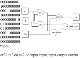
Figure 2: Full adder represented as a circuit adjacency matrix. The circuit is shown as gates on the right here as an illustration, this is not typically included in a circuit adjacency matrix.

Trigger Generation: Combinatorial and sequential triggers are generated as follows. For a combinatorial trigger, we specify the number of inputs desired. Then we create a tree structure starting with a single gate as the root node and continuing until the desired number of inputs has been achieved. Each node is randomly selected as either an AND gate, a NOT gate or an INPUT. AND gates have two child nodes, while NOT gates have one, and INPUTS are leaf nodes. When each leaf node is an INPUT the trigger structure is complete. Trees with incorrect number of INPUT nodes or ones where not all leaf nodes are INPUT, are discarded. In order to generate sequential triggers, we compile a script, which for a given sequence, generates a Verilog HDL code for a non-overlapping Mealy sequence. This HDL code is then synthesized to a gate-level netlist and then converted to circuit adjacency matrix.

Triggers thus generated are structurally and functionally representative of different types of combinatorial and sequential triggers that can be used in trigger-based HT [27]. For a combinatorial trigger, trigger size is equal to the number of inputs of the trigger and for a sequential trigger, it refers to the number of flipflops in the trigger circuit (equivalent to base-2 logarithm of input sequence length).

Trigger Embedding: Circuit adjacency matrices are then embedded with triggers by appropriately adding rows and columns equivalent to number of trigger nodes and creating appropriate connections between trigger inputs and randomly selected insertion nodes of the benign circuit adjacency matrix. In this way, each adjacency matrix is embedded with each trigger to yield multiple HT embedded adjacency matrices.

Inverse Node Fanin: These trigger-embedded circuit adjacency matrices are used as the starting point to extract inverse node fanins (INF). The INF of a node $i$ in $A$ is a subgraph consisting of all paths starting at a circuit input and terminating at $i$. The INF for a node is an effective representation of its neighborhood. An entire circuit can be described by specifying the INF for each node in the circuit. INFs for all circuit nodes are generated in a straight-forward manner from circuit adjacency matrices. For a graph of an HT-embedded circuit, we define trigger INF as the INF of the node corresponding to the output of the trigger and benign INFs as the INFs of all the other nodes in the graph. Note that some benign INFs may contain a few trigger nodes but never the complete trigger.

III HT Trigger Detection with GATE-Net 

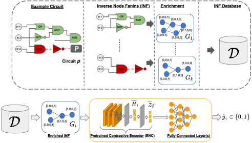
Figure 3:  GATE-Net : Graph-Aware Trigger Detection Network . Here, we illustrate the classification pipeline with the help of an example circuit. A circuit $p$ with $k$ cells in it’s netlist is broken down into $k$ INFs. Each INF is enriched with cell-types (one-hot encoding). Enriched INFs are represented as INF database $\mathcal{D}$. Each INF in $\mathcal{D}$ is passed into the classification model (orange box), wherein a latent representation $\bar{z}_{i}$ is obtained from the pretrained contrastive encoder (ENC). $\bar{z}_{i}$ is then supplied to a fully connected network (FCN) to obtain the final classification $\hat{\mathrm{y}}_{i}\,$ for $G_{i}$. The classification model consists of a contrastive encoder (ENC) (detailed in section. III-A) and a set of fully connected layers. The proposed classification pipeline is hence dependent ONLY on information available in the netlist and no further feature engineering is required.

A synthesized circuit can be viewed as a directed acyclic graph, hence we exploit GCN models which have demonstrated effectiveness in the context of unstructured data for effective HT trigger detection. Details about the GCN learning mechanism are provided in [22].

Let us consider a dataset $\mathcal{C}=\{C_{1},C_{2},...,C_{N}\}$ of hardware circuits, with each circuit potentially having a HT with a trigger and a payload embedded. Let us consider a circuit $C_{p}\in\mathcal{C}$; an HT embedded in $C_{p}$ comprises the trigger $t_{p}$ connected at one or more nets in $C_{p}$. Trigger $t_{p}$ is activated by a specific input pattern. Upon activation, $t_{p}$ activates the attached payload. We wish to detect the presence of HT in $C_{p}$ by training a learning model to detect $t_{p}$. Our learning model is trained only on the circuit’s netlist and we do not use any other features other than the gate-types of each gate in $C_{p}$. This deliberate restriction of our approach (i.e., to only use information available from the circuit netlist) is to ensure avoidance of cost associated with rich feature engineering pipelines that have been employed by previously proposed HT detection methods [13, 12, 19, 28, 15], preventing these methods from scaling to large circuit databases.

Fig. 3 depicts the full classification pipeline for HT trigger detection that we employ. We first extract INF for all nodes from the adjacency matrix representation of $C_{p}$ as outlined in Section II. Let $G^{p}_{i}$ be the INF of node $i$ for circuit $p$. $G^{p}_{i}$ is now considered a graph where each node (a cell in the original $C_{p}$) is enriched (tagged) with a one-hot vector indicating its cell-type. INF extraction and node-enrichment for each circuit in $C$ results in a dataset $\mathcal{D}=\{G^{1}_{1},..,G^{1}_{|V_{1}|},..,G^{p}_{1},..,G^{p}_{|V_{p}|},..,G^{N}_{|V_{N}|}\}$. Here, $|V_{i}|$ is the number of cells in $C_{i}$ (or nodes in $A_{i}$). Without loss of generality we can consider $\mathcal{D}$ to be a dataset of $m$ INFs $\mathcal{D}=\{G_{1},...,G_{m}\}$ extracted from all circuits in $\mathcal{C}$. In this work, we consider each $G_{i}$ to be an undirected graph. Our GATE-Net model is trained in a supervised manner to classify each graph $G_{i}$ as a benign or a trigger INF.

We can define the binary cross-entropy loss function to train GATE-Net for the task of HT detection as

$$\small\begin{split}\mathcal{L}&=-\frac{1}{m}\sum_{i=1}^{m}\mathrm{y}_{i}\mathrm{\textbf{ln}}(\hat{\mathrm{y}}_{i})+(1-\mathrm{y}_{i})\mathrm{\textbf{ln}}(1-\hat{\mathrm{y}}_{i})\\ \hat{\mathrm{y}}_{i}&=f_{\Theta}(\mathbf{x}_{i},\mathbf{A}_{i})\end{split}$$ (1)

where $f_{\Theta}$ represents the GATE-Net learning model comprised of a set of parameters $\Theta=\{\theta^{(1)},\theta^{(2)},..,\theta^{(L)}\}$ where each $\theta^{(r)}$ represents parameters for layer $r$. $f_{\Theta}$ is a function of $\mathbf{A}_{i}\in\mathbb{B}^{l\times l}$ the adjacency matrix of $G_{i}$ (assume $G_{i}$ has $l$ nodes) and $\mathbf{x}_{i}\in R^{l\times 1}$, a vector of node features (indicating cell-type) for each node in $G_{i}$. Note, although we employ only one-hot encoding of cell-types in this work, $\mathbf{x}_{i}$ can quite easily be augmented to include richer features if available, thereby making GATE-Net , a generic framework for representation learning for hardware circuits useful for various detection tasks.

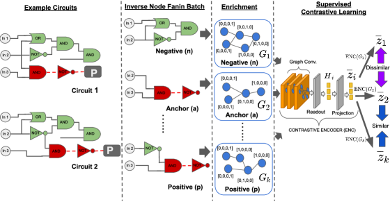
Figure 4: We illustrate the contrastive learning pipeline with an example scenario wherein $\mathcal{C}$ consists of only two circuits, each circuit broken down into INFs and corresponding enriched graphs to yield a total of $k$ INFs $\mathcal{D}=\{G_{1},..,G_{k}\}$. Specifically, we consider the effect of contrastive learning for the fanin $G_{2}$ i.e., the trigger fanin from circuit 1 (which is called the anchor (a) in contrastive learning parlance). Here, fanin $G_{k}$ (positive (p) in contrastive learning parlance) has the same label (i.e., belongs to the same class) as $G_{2}$, hence the contrastive loss (Eq. 3) constrains $\overline{z}_{2}$ and $\overline{z}_{k}$ to be similar while causing $\overline{z}_{1}$ (representation for $G_{1}$; called negative (n) instance in contrastive learning parlance) to be dissimilar to both $\overline{z}_{2}$ and $\overline{z}_{k}$.

III-A Supervised Contrastive Pretraining

Our GATE-Net model consists of two parts (i) a contrastive encoder (ENC) (inspired from the supervised contrastive learning model proposed by Khosla et al. in [8] for image classification) followed by (ii) multiple fully connected layers (FCN).

Embedding: The first part of ENC, consists of learning a latent embedding for the input graph $G_{i}$ which is achieved through three Graph Convolutional Network (GCN) layers interleaved with ReLU activation functions [29]. Each GCN layer involves a topology-aware representation learning mechanism.

$$\small H^{(r+1)}=\mathrm{ReLU}(D_{i}^{\frac{1}{2}}A_{i}D_{i}^{\frac{1}{2}}H^{(r)}\theta^{(r)})$$ (2)

In Eq. 2, $\mathrm{H}^{(r)}$ corresponds to the latent representation in the $r^{th}$ layer. $H^{(0)}=\mathbf{X}_{i}\in\mathbf{R^{l\times l}}$ (i.e., one-hot encodings for all nodes in $G_{i}$). $D_{i}$ is the degree matrix of $G_{i}$ and $\theta^{(r)}$ is the set of weights corresponding to layer $r$. The term $D_{i}^{\frac{1}{2}}A_{i}D_{i}^{\frac{1}{2}}$ indicates the symmetric normalized Laplacian matrix of $A_{i}$ and encodes the rich connectedness structure of the graph which is useful for propagating the node representations appropriately from one GCN layer to the next while also being employed in the message passing of node representations (details in  [22]). Intuitively, the $r^{th}$ GCN layer learns node embeddings (for all nodes in $G_{i}$) influenced by neighbors up to $r$-hops away.

Our GATE-Net model consists of three GCN layers and hence considers effects of nodes up to 3-hops away. These GCN layers yield a set of 3 latent representations $\{H^{(1)},..,H^{(3)}\}$. The latent representation $H_{3}\in\mathbb{R}^{l\times q}$ where $q$ represents the latent dimension and $l$ the number of nodes in $G_{i}$. $H_{3}$ is hence a matrix consisting of a q-dimensional latent representation for each node in $G_{i}$. A readout step is employed to transform these individual node-representations present in $H_{3}$ into a single representation $\overline{H}_{i}\in\mathbb{R}^{q\times 1}$ for the entire graph $G_{i}$. In GATE-Net , we employ mean pooling as the choice of readout layer and hence our final graph representation $\overline{H}_{i}$ is an element-wise mean of all the individual node representations present in $H_{3}$.

Projection: The second part of ENC comprises a linear transformation of $\overline{H}_{i}$ (normalized to lie on the unit hypersphere) to obtain a projected representation $\overline{z}_{i}\in\mathbb{R}^{q^{\prime}\times 1}$, in our case $q^{\prime}$ is the latent projection dimension set to 256. Hence, for each INF graph $G_{i}$ with $l$ nodes, the ENC yields a latent representation $\overline{z}_{i}\in\mathbb{R}^{q^{\prime}\times 1}$ projected onto the unit hypersphere.

Contrastive Loss Formulation: Most contrastive learning approaches proposed thus far [24, 25], have been unsupervised (or more specifically “self-supervised”) and due to the absence of explicit instance labels, rely on manipulating the input instance i.e., (cropping in case of images; adding or deleting nodes/edges in the case of graphs), and ensuring similar representations obtained for the original and manipulated instance. Overall, it has been found that contrastive learning approaches influence the learned representation (and improve model prediction quality) by lending greater structure to the latent space learned by the model.

In Fig. 4, an illustrative example of the effect of contrastive learning is presented. Let us consider a scenario with $\mathcal{C}$ comprising only of two circuits. Each circuit is broken down into its INFs and each node in every INF is enriched with its cell-type, as described previously in section III to obtain a dataset $\mathcal{D}$ of input graphs. Let us consider $\mathcal{D}=\{G_{1},...,G_{k}\}$ to comprise of $k$ INFs from circuits in $\mathcal{C}$. Since each of the two circuits in $\mathcal{C}$, has a trigger embedded, each circuit has a single INF which is labeled a trigger INF while the rest are benign INFs.

Each $G_{i}\in\mathcal{D}$ is operated on by the contrastive encoder (ENC) in GATE-Net , to obtain a set ${Z=\{\overline{z}_{1},\overline{z}_{2},..,\overline{z}_{k}|\overline{z}_{i}\in\mathbb{R}^{q^{\prime}\times 1}\}}$ of projected representation vectors on the unit hypersphere. Owing to our supervised problem context, there also exist a set of corresponding labels $\mathrm{Y}=\{\mathrm{y}_{1},..,\mathrm{y}_{\mathrm{k}}\}$ such that $\mathrm{y}_{i}\in\{0,1\}$. Given, $\mathcal{D},\mathrm{Z},\mathrm{Y}$, our supervised contrastive loss is described in Eq. 3

$$\small\sum\limits_{G_{i}\in\mathcal{D}}\frac{-1}{|P(i)|}\sum\limits_{p\in P(i)}\mathrm{log}\frac{\mathrm{exp}(\mathrm{z}_{i}\boldsymbol{\cdot}z_{p}/\tau)}{\sum\limits_{G_{j}\in\mathcal{D}^{\prime}(i)}\mathrm{exp}(z_{i}\boldsymbol{\cdot}z_{j}/\tau)}$$ (3)

Here, for each graph $G_{i}\in\mathcal{D}$ (note $G_{i}$ is referred to as the anchor graph), the set $P(i)$ includes all instances in $\mathcal{D}$ that have the same class label as $G_{i}$. Each member of $P(i)$ is considered a positive instance (in contrastive learning parlance) w.r.t the anchor instance $G_{i}$. The numerator of the logarithm in Eq. 3, calculates the dot product between the ENC generated latent representation of $G_{i}$ and ENC generated latent representation obtained for positive graph $G_{p}\in P(i)$. The denominator is a normalizing constant and is a summation of similar dot-products between $G_{i}$ and all other instances in $\mathcal{D}$ excluding $G_{i}$ (i.e., with all members in set ${\mathcal{D}^{\prime}(i)=\mathcal{D}\setminus\{G_{i}\}}$). Intuitively, Eq. 3 encourages representations $z_{i}$ belonging to the same class to be closer together while actively separating representations of different classes to be far apart. Hence, the goal of supervised contrastive learning coincides well with the general goal of classification pipelines which is to learn latent representations easily separable by a hyperplane between the various classes.

Pretraining: Hence, we employ the aforementioned supervised contrastive learning procedure as a pretraining step in our classification pipeline. Essentially this means, that the ENC model is first trained using the contrastive loss function in Eq. 3 after which the trained layers in ENC are frozen (i.e., the weights are unaffected by backpropagation).

Classification: This frozen ENC module is then combined with a 3-layer fully-connected network (FCN) which finally transforms $\overline{z}_{i}$ (i.e., each output of ENC) to predict the probability of $G_{i}$ containing a trigger.

IV Experimental Setup and Evaluation

We now detail the data used for training and evaluation of GATE-Net and also outline the evaluation procedure.

IV-A Dataset Description

In order to train GATE-Net to recognize trigger-based HTs, we required a database of circuits to be embedded with the triggers we generated. For this purpose, we use the open-source IP cores from Opencores.org [30]. The cores are compiled and synthesized to flattenned gate-level netlists using a standard CMOS cell library [31]. Of all the available standard cells in the library, we use only the basic set of cells, comprising of logic gates: AND, OR and NOT and flipflops: D-Flipflop, D-Flipflop with asynchronous reset and D-Flipflop with asynchronous set and asynchronous reset. The restriction to a limited set of cells is done to have structural similarity with the HT triggers discussed in Section II, thereby, not making the detection easier. We used IP cores written in Verilog HDL and Synopsys DC compiler [32] as synthesis tools. GATE-Net only requires synthesized flattened netlist Generally, our approach can be applied for netlist synthesis from any standard cell library and is independent of synthesis tools and HDL (Verilog/VHDL).

TABLE I: Evaluation dataset: Types of IP cores and total cell count

No.	IP Core description	Total Num. cells
1	Antilogarithm function	912
2	Logarithm function	441
3	Cellular automata pseudo random number generator	931
4	Simple serial peripheral interface (SPI)	968
5	Fixed point arithmetic module	2362
6	Wishbone to LPC bridge	723
7	Simon block cipher	1443
8	Wishbone controlled FM transmission	1445
9	Wishbone to AXI	1355
10	Digital phased lock loop	503
11	I2C slave	908
12	Random number generator	587
13	SPI-3 interface	709
14	Vedic mathermatics	827
15	USB host controller	10781
16	Hight block cipher	4534
17	Context adaptive variable length coding	5407
18	Signed division	4691

The set of IP cores used in evaluation and their size in terms of number of cells is shown in Table I. Each IP core is a benign circuit, synthesized and converted to the adjacency matrix representation and a HT trigger is inserted at a random insertion point. For each benign circuit, multiple instances of trigger-embedded circuits are generated with a distinct trigger and at distinct insertion points. We further divide the dataset for our HT detection experiments into: a) a dataset consisting of benign circuits embedded with combinatorial triggers and b) a dataset consisting of benign circuits embedded with sequential triggers. The procedure outlined in Section II is used to embed triggers of sizes 15–35 for combinatorial and 3–5 for sequential triggers. The INFs for both datasets are then extracted. Table II details the distribution of benign and trigger INFs in each dataset. We retain the imbalanced distribution of benign and trigger INFs to maintain a realistic, challenging classification setting.

We plan to publicly release a larger dataset, comprising of 58 IP cores, and comprehensive in terms of a) circuit sizes: the number of cells in synthesized gate-level netlists ranges from 200 to 200000; and b) application area: arithmetic, communication, and encryption, among others.

TABLE II: Dataset Statistics

Dataset	Experiment Type	Benign Fanins	Trigger Fanins
Comb. Triggers	Train	2161	1485
	Test	2222	232
Seq. Triggers	Train	1145	723
	Test	2977	2470

IV-B Testing Environments

We use the following two environments to test and compare GATE-Net with existing state of the art (SOTA) approaches:

Random-Shuffle Testing: In this type of testing, we randomly assign INFs to the training and testing sets. This would imply the possibility of benign INFs from the same circuit present in both training and testing sets. However, the actual INFs are NOT identical as each node has a unique INF and the INF for each node in a circuit is used ONLY once either in training or testing (never both). By the same reasoning, the trigger INFs will also be distinct in both the sets, where at best, the same trigger embedded in a different benign circuit can be encountered in both the sets.

Extrapolation-Based Testing: We also create a significantly more challenging testing scenario to gauge the power of strict extrapolation of the models considered. Here, we ensure that INFs in training and testing sets arise from disjoint sets of circuits. Furthermore, a trigger seen during training is never encountered during testing (not even embedded in a different circuit); in particular, triggers of different sizes are employed for training and test to ensure this. The circuits #1–#5 and #12–#18 of Table I are used in the training and the rest are used for testing. The circuits in training are embedded with combinatorial triggers of sizes 20–35 and sequential triggers of sizes 4,5 and circuits in testing with combinatorial triggers of sizes 10,15 and sequential triggers of size 3.

IV-C Evaluation

To inspect representation learning capability of GATE-Net , we compare it’s performance on the task of HT detection with standard SOTA classifiers presented by Kurihara et al. [15] and Hoque et al. [19]. For this purpose, we use the dataset comprising of IP cores numbered 1–7 from Table I, each embedded with 21 combinatorial triggers and 30 sequential triggers, thereby generating a total of 357 instances of trigger-embedded circuits (INF statistics in Table III). For each of these instances, we extract various structural and functional features presented in [15] and [19], shown in Table IV.

TABLE III: Dataset statistics for comparison against state-of-the-art approaches. Due to the expensive feature engineering required for Hoque et al. [19] and Kurihara et al. [15], models, it was intractable to evaluate them on the full dataset (Table II) and we hence employ a smaller subset for SOTA comparison.

Dataset	Experiment Type	Benign Fanins	Trigger Fanins
Comb. Triggers	Train	3138	126
	Test	768	29
Seq. Triggers	Train	3211	163
	Test	788	47

Kurihara et al. [15]: This approach uses 11 structural features to classify whether a net is a HT net or a normal net. We have extracted these features for each net in our gate-level netlists. The exceptions being feature #9, as the output of the trigger in our representation does not connect to the circuit, and feature #11 because we do not use multiplexers in our synthesized gate-level netlist.

Hoque et al. [19]: This approach uses 5 structural features and 9 functional features to classify whether a net is a HT net or a normal net. The structural features, #1–#4 are extracted from the gate-level netlist for each net and feature #5 is not used for the reason discussed above. The functional features, #6–#9 are extracted by synthesizing the HT-embedded circuits in the Xilinx Vivado tool by using the command report_switching_activity for each net. As only 2-input logic gates and D-flipflops are used in our approach, feature #10 is set to 1 for all nets. The controllability-based features, #11–#14 are not considered because the control value based identification, derived from boolean functional analysis, has limitations against HTs with sequential triggers as they are triggered by an input stream over a period of time [9].

The features, thus extracted, are assigned to each node in the adjacency matrix representation and the INFs are generated. Each node in the INFs is then passed on to the classifiers (used in [15] and [19] respectively). If more than 5% of the nodes in an INF are classified as trigger nodes, then the INF is detected as trigger INF.

TABLE IV: Structurual and Functional Features used in the State of the Art approaches

No.	Kurihara et al. [15]	Hoque et al. [19]
1	No. of immediate fan-in upto 4-level away from input side of net	No. of immediate fan-in of net
2	No. of immediate fan-in upto 5-level away from input side of net	No. of immediate fan-out of net
3	No. of flipflops upto 4-level away from input side of net	Cell type driving the net
4	No. of flipflops upto 3-level away from output side of net	Min. distance from primary input
5	No. of flipflops upto 4-level away from output side of net	Min. distance from primary output
6	No. of 4-level loops on the input side of net	Static probability
7	No. of 5-level loops on the output side of net	Signal rate
8	Min. levels to primary input	Toggle rate
9	Min. distance to primary output	Min. toggle rate
10	Min. levels to nearest flipflop	Entropy of the driver function
11	Min. levels to nearest multiplexer	Lowest controllability of inputs
12–14	–	Highest, average and standard deviation of controllability of inputs

Evaluation Metrics: We employ standard classification metrics precision (Prec), recall (Rec), F1 score [33] for evaluating model performance. Intuitively, precision penalizes the models for false positive classifications, i.e., classifying benign fanins as trigger fanins, while recall represents the proportion of all trigger fanins correctly identified by the model.

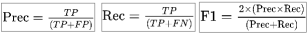
Figure 5: Evaluation Metrics.

The F1 score (range [0,1]) is the harmonic mean of precision and recall and a good indication of overall accuracy. In Fig. 5, TP, FP, FN indicate true-positive (i.e., trigger INF that is correctly identified), false-positive (benign INF falsely identified as trigger INF) and false-negative (trigger INF falsely identified as benign INF) classifications respectively.

V Results and Discussion

To evaluate the representation learning capability of GATE-Net , we conduct a performance comparison on a downstream task of HT detection for a variety of hardware circuits embedded with combinatorial and sequential triggers. In each case, we compare GATE-Net with state-of-the-art classification models, namely Kurihara et al. [15] and Hoque et al. [19]. Each of the aforementioned state-of-the-art baseline HT detection approaches involve extensive feature-engineering and extract various structural and functional features of the circuit which are then employed in the HT detection task as described in section IV-C. Our GATE-Net model on the other hand only uses the graph structure of each INF (section III) enriched with cell-types (i.e., all information available directly form the netlist).

Specifically, we inspect three aspects to verify the effectiveness of our proposed GATE-Net model:

1. Performance of GATE-Net compared to state-of-the-art HT detection techniques for combinatorial and sequential triggers embedded in INFs.

2. Effectiveness of contrastive learning of GATE-Net evaluated on a large expanded dataset comprising multiple trigger types and multiple groups of benign circuits, compared to a variant without contrastive learning for combinatorial and sequential INFs.

3. Finally, we also characterize the performance of GATE-Net on an extremely challenging extrapolation setting for a holistic analysis of performance.

V-A Comparison with State of the Art

We characterize the performance of our proposed GATE-Net architecture relative to state of the art HT detection models proposed by Kurihara et al. [15] in Table V. The comparison is performed in the context of detecting combinatorial as well as sequential triggers embedded in hardware circuits. We notice that in both cases GATE-Net is able to outperform the model proposed by Kurihara et al. [15] significantly.

TABLE V: Comparison of GATE-Net with a state of the art HT detection model presented by Kurihara et al. [15].

Expt. Type	Model	Precision	Recall	F1
Combinatorial	GATE-Net	0.95	0.9	0.87
	GATE-Net -noCont.	0	0	0
	Kurihara et al. [15]	0.83	0.4	0.54
Sequential	GATE-Net	1	0.92	0.96
	GATE-Net -noCont.	1	0.5	0.67
	Kurihara et al. [15]	0.68	0.87	0.76

Specifically, we notice that our model outperforms theirs by 61.11% on the F1 score metric for combinatorial triggers and by 26.32% for sequential trigger detection, in both cases yielding significant performance improvement over the state of the art model. In the case of combinatorial trigger detection (which from the results may be inferred to be the harder of the two tasks), there is a significant deterioration in the recall of the Kurihara et al. [15] model which is the main reason for performance degradation which indicates that this model is able to correctly identify only about 40% of the triggers in the combinatorial fanin dataset. There is also a drop in the precision of the Kurihara et al. [15] model for the sequential trigger detection task which is caused by the model detecting many false positives and from the table it may be inferred that the model is only correct 68% of the time where it identifies an INF as containing a sequential trigger. Such a high false positive rate may be costly. GATE-Net on the otherhand is able to achieve very high precision (i.e., low false positive rates) and recall (i.e., able to identify all the variety of triggers) for both combinatorial and sequential trigger datasets.

TABLE VI: Comparison of GATE-Net with a state of the art HT detection model presented by Hoque et al. [19]

Expt. Type	Model	Precision	Recall	F1
Combinatorial	GATE-Net	0.96	0.9	0.93
	GATE-Net -noCont.	0	0	0
	Hoque et al. [19]	0.94	0.55	0.7
Sequential	GATE-Net	1	0.89	0.94
	GATE-Net -noCont.	0.95	0.79	0.86
	Hoque et al. [19]	0.97	0.68	0.8

In Table VI, we compare the GATE-Net model with another state-of-the-art HT detection model proposed by Hoque et al. [19], once again evaluating all models in the context of detecting combinatorial and sequential trigger INFs. We once again observe that GATE-Net is able to outperform the state-of-the-art model by Hoque et al. [19] on both combinatorial and sequential HT deteciton tasks. However, unlike the Kurihara et al. model, we notice that the model proposed by Hoque et al. [19] has high precision (i.e., low false positive rates) in both combinatorial and sequential HT detection cases. This may be attributed to the fact that the classification model in this case is actually an ensemble of three classifiers (i.e., Random Forest, Gradient Boosting, Naive Bayes) which is provably superior than the individual Random Forest model employed by Kurihara et al. [15]. However, we notice that even in this case, the GATE-Net model outperforms the state of the art HT detection model by Hoque et al. [19] by 32.86% for combinatorial HT detection and by 17.5% for sequential HT detection. Once again the deterioration in performance of Hoque et al. [19] may be attributed to its inability to identify the variety of triggers resulting in the low recall value in both combinatorial and sequential HT detection contexts.

Finally, we also compared the GATE-Net -noCont. model which is a variant of the GATE-Net without the supervised contrastive pretraining phase. We observe some interesting trends consistent across Table V and Table VI. In both cases, we notice that the model is unable to recognize ANY combinatorial triggers. This may be attribured to the drastic data imbalance between the benign and trigger INFs during the training context of all models. It is interesting to note that contrastive learning in addition to allowing the model to learn better quality representations is also able to perform effectively in data imbalance contexts which is apparent from the results in both these tables by comparing performances of GATE-Net with GATE-Net -noCont. However, we also notice that GATE-Net -noCont. is able to yield a somewhat improved performance for the sequential HT detection task although still inferior to GATE-Net . We further investigate this comparative behavior between GATE-Net and its variant without contrastive learning in sec. V-B. Note that although both Table V and Table VI use datasets derived from the one detailed in Table III, due to the stochasticity in sampling of benign INFs for very large circuits (i.e., only INFs from a subset of benign nodes are sampled to make the INF extraction process tractable), the specific subsets of data may be slightly different although the overall data characteristics and experimental settings are identical across the two settings.

V-B Effectiveness of Contrastive Learning

In order to test the effect of contrastive learning, we evaluate the GATE-Net and GATE-Net -noCont. models on much larger datasets for combinatorial and sequential HT detection. To simulate data paucity, we use only 40% of the available data for training and the rest of the data is used for performance evaluation in this experiment.

TABLE VII: Effectiveness of Contrastive Learning in GATE-Net . We notice that GATE-Net outperforms variant without contrastive learning GATE-Net -noCont. in detection of both sequential and combinatorial triggers.

Expt. Type	Model	Precision	Recall	F1
Combinatorial	GATE-Net	0.99	0.98	0.99
	GATE-Net -noCont.	0.93	0.72	0.81
Sequential	GATE-Net	0.96	0.94	0.95
	GATE-Net -noCont.	0.9	0.95	0.92

In Table VII, we notice that GATE-Net i.e., the model with constrastive learning (pre-training) outperforms the variant without constastive learning i.e., GATE-Net -noCont. We also notice that the performance of the variant of GATE-Net without constastive learning deteriorates significantly for the combinatorial trigger detection task while the performance of GATE-Net with constrastive learning remains relatively consistent for both the trigger types, indicating that contrastive learning helps GATE-Net learn generalizable, robust representations of INFs for HT detection. We also notice that in the case of combinatorial trigger detection, the variant of GATE-Net without contrastive learning has low recall which implies that it is unable to recognize many of the variety of triggers present in the dataset while GATE-Net (i.e., with constrastive learning) is able to recall (i.e., correctly identify) 98% of the triggers in the dataset further showcasing the power of contrastive learning to enable models to learn highly generalizable representations. We see that GATE-Net outperforms its variant without contrastive learning by 22.22% for combinatorial HT detection and by 3.26% for the sequential HT detection. Fig. 6–6 qualitatively demonstrate the effect supervised contrastive pretraining has on the GATE-Net model representation thereby leading to superior performance over GATE-Net -noCont.

(a) Epoch 0

(b) Epoch 50

(c) Epoch 100

(d) Epoch 150

Figure 6: Principal Component Analysis (PCA) reduced 2D embeddings of the representations $\overline{z}_{i}$ incrementally learnt by GATE-Net ENC model during contrastive pretraining over the course of 150 epochs. We notice that embeddings of benign INFs (green) and trigger INFs (red), start from a random projection setup before training at Epoch 0 (a), and are increasingly separated ultimately leading to the maximally separated representation seen in (d). This illustrates the effect of contrastive learning in the GATE-Net pipeline. Such explicitly separable embeddings are absent in GATE-Net -noCont. leading to inferior performance.

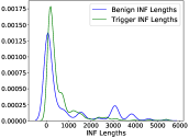
(a)

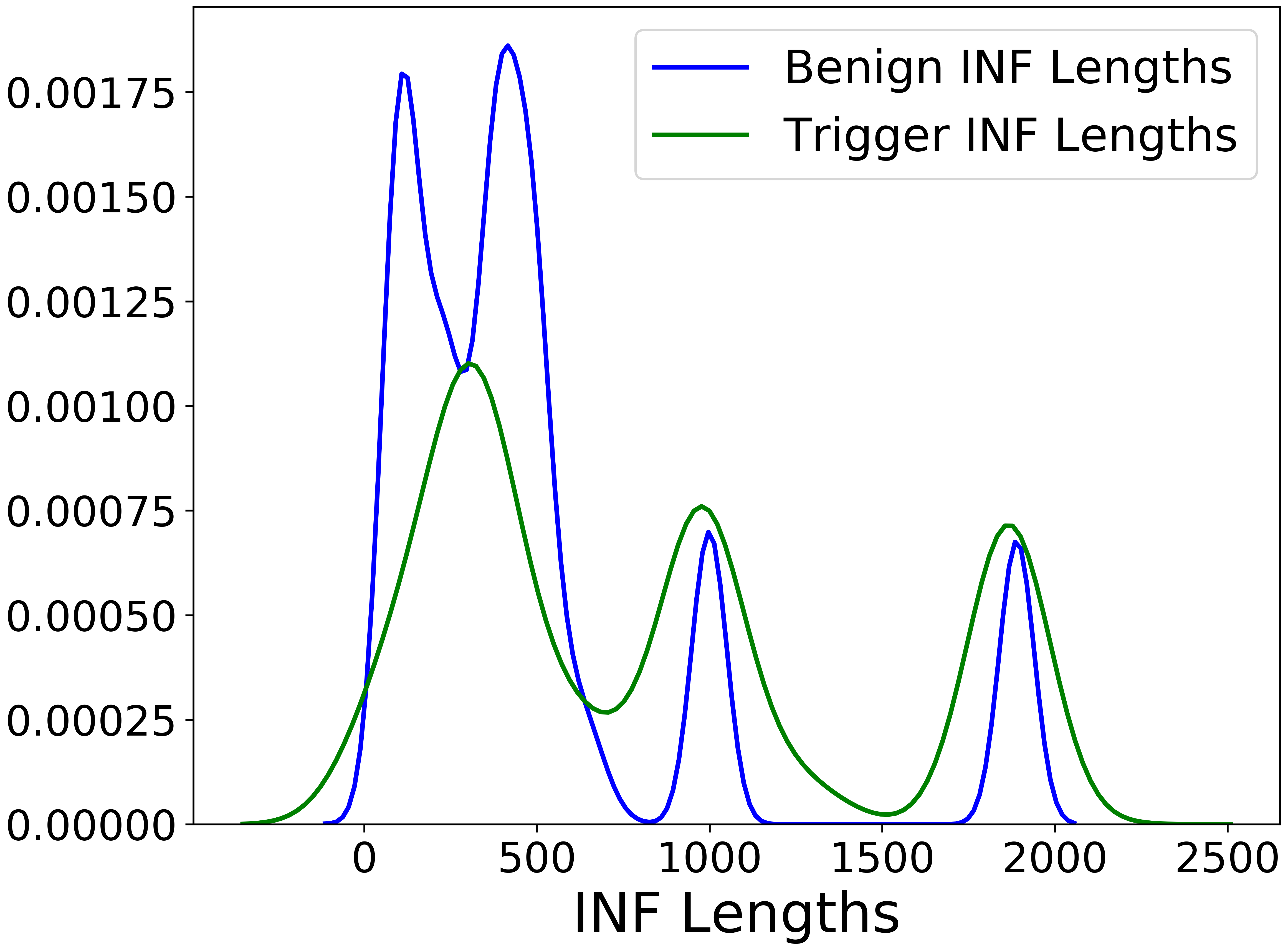
(b)

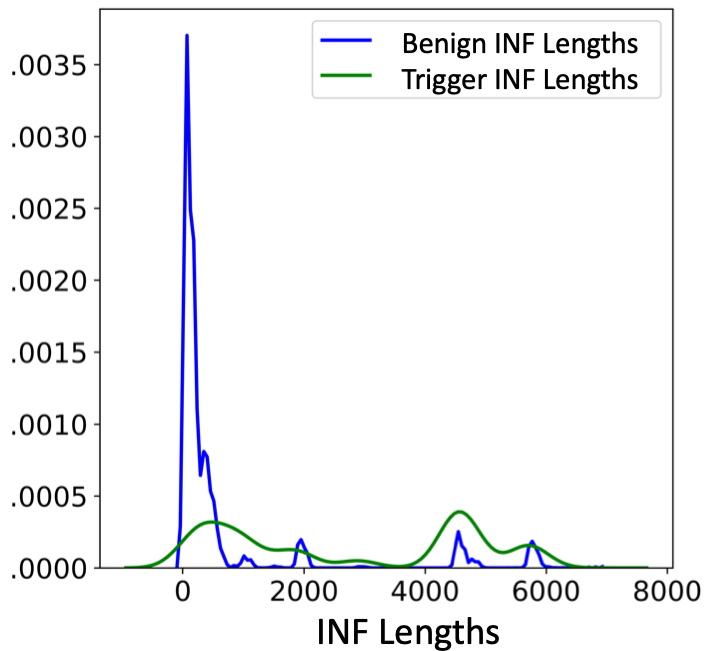
(c)

Figure 7: (a) INF length distribution random trigger insertion on synthetic data consisting only of AND,OR,NOT gates and combinatorial triggers. (b) INF length distribution on real circuit data embedded with comb. triggers with shallow trigger embedding (c) INF length distribution on real circuit data embedded with seq. triggers with shallow trigger embedding.

V-C Extrapolation Performance

We now evaluate the out-of-distribution generalization performance of GATE-Net , without explicitly training GATE-Net for this challenging experimental setting to understand out of the box behavior in this context and also to evaluate the effectiveness of contrastive learning in this context. To simulate out-of-distribution evaluation, we train our models only on a subset of the benign circuits and trigger sizes and evaluate model performance on triggers of different sizes embedded in completely different benign circuits.

TABLE VIII: Effectiveness of GATE-Net for out-of-distribution generalization compared with GATE-Net -noCont.

Expt. Type	Model	Precision	Recall	F1
Combinatorial	GATE-Net	0.38	0.67	0.48
	GATE-Net -noCont.	0.3	0.66	0.42
Sequential	GATE-Net	0.54	0.78	0.64
	GATE-Net -noCont.	0.51	0.82	0.63

We notice from Table VIII that both GATE-Net and GATE-Net -noCont. experience significant performance deterioration in the out-of-distribution extrapolation context. Specifically, the most significant deterioration occurs in the context of combinatorial HT detection which has been previously established to be the harder of the two detection tasks evaluated in this work. However, we still notice that in both cases, the F1 score of GATE-Net is higher than the variant without contrastive learning although the performance difference observed previously between the two models dwindled in the extrapolation setting inspected here. Our goal of evaluating GATE-Net in this challenging extrapolation context is not to display state-of-the-art performance results but rather to establish a baseline of performance of an out of the box model (GATE-Net ) which has not been explicitly trained to excel in out-of-distribution generalization tasks so future efforts may build upon our pipeline to improve performance.

Results Summary: GATE-Net outperforms all SOTA classification models compared for HT detection. Hence, our results demonstrate superior representation learning capacity of GATE-Net , for HT detection. Overall, we achieve an average 46.99% performance improvement in F1 score over the two SOTA baselines for detection of combinatorial triggers and 21.91% improvement for detecting sequential triggers. We also inferred from the results that contrastive learning is very effective in allowing GATE-Net to learn robust, generalizable representations even in the context of data paucity. As apparent from Table. VII, GATE-Net achieves average performance improvement of 12.74% in F1 score across combinatorial and sequential HT detection.

Security Analysis: We now evaluate effects of various trigger embedding procedures and their effect on the degree of difficulty in HT detection. One approach is to randomly embed triggers, wherein a trigger with $k$ inputs has $k$ randomly chosen circuit nets connected to it. An experiment on a simple dataset of circuits (consisting only of AND,OR and NOT gates) with randomly embedded triggers reveals interesting insights about the resulting INFs. In Fig. 7(a), We observe a noticeable difference in the models of INF length distributions for both benign and trigger INFs. Also, INF lengths of size 2500 and above may be safely be regarded as benign (a trivial but effective detection strategy in this case). To avoid such biases in INF length, we assume a sophisticated attacker who has control over the trigger embedding process and adopts a shallow embedding strategy wherein the trigger is embedded at most $k$-hops ($k=2$ in our case) away from circuit inputs. This strategy alleviates discrepancy in INF length distributions between trigger and benign INFs, see Fig. 7(b) and Fig. 7(c) which both show much better agreement between INF length densities between trigger and benign INFs for combinatorial and sequential triggers respectively. Triggers so embedded are harder to detect with trivial features like INF lengths.

VI Conclusion

In this paper we proposed GATE-Net , a novel machine learning model based on supervised contrastive pre-training and graph convolutional networks for HT detection employing only data available from the circuit netlist. Through rigorous experimentation and comparison with several state-of-the-art baseline models we show that GATE-Net achieves significantly better results for HT detection over a wide variety of circuit types with randomly embedded combinatorial (46.99% performance improvement over baselines) and sequential triggers (21.91% performance improvement over baselines). We also extensively evaluate the effect of supervised contrastive learning in GATE-Net and compare it with a variant of GATE-Net without contrastive learning and show qualitatively and quantitatively that supervised contrastive learning helps GATE-Net yield superior performance for HT detection. We also proposed and detailed a methodology for generating and representing circuits embedded with HT triggers and have publicly released data and code for GATE-Net , trigger generation and embedding. We also performed analysis of out-of-distribution generalization performance of GATE-Net to serve as an effective baseline for future HT detection endeavors. Finally, we performed a security analysis and detail advantages of a shallow trigger embedding procedure for better trigger masking in the circuits. In the future, we wish to extend our current GATE-Net approach and characterize its performance in the context of adversarial trigger generation models.

Acknowledgements: This work is supported in part by the National Science Foundation via grant DGE-1545362.

References

- [1] M. Tehranipoor and F. Koushanfar, “A survey of hardware trojan taxonomy and detection,” IEEE design & test of computers, vol. 27, no. 1, 2010.
- [2] Z. Huang et al., “A survey on machine learning against hardware trojan attacks: Recent advances and challenges,” IEEE Access, vol. 8, pp. 10 796–10 826, 2020.
- [3] H. Li et al., “A survey of hardware trojan detection, diagnosis and prevention,” in IEEE CAD/Graphics, 2015, pp. 173–180.
- [4] D. Agrawal et al., “Trojan detection using ic fingerprinting,” in IEEE SP’07, 2007, pp. 296–310.
- [5] R. S. Chakraborty et al., “Mero: A statistical approach for hardware trojan detection,” in Springer CHES, 2009, pp. 396–410.
- [6] R. S. Chakraborty, S. Narasimhan, and S. Bhunia, “Hardware trojan: Threats and emerging solutions,” in 2009 IEEE HLDVT, 2009, pp. 166–171.
- [7] F. Courbon et al., “A high efficiency hardware trojan detection technique based on fast sem imaging,” in DATE, 2015, pp. 788–793.
- [8] P. Khosla, P. Teterwak, C. Wang, A. Sarna, Y. Tian, P. Isola, A. Maschinot, C. Liu, and D. Krishnan, “Supervised contrastive learning,” arXiv preprint arXiv:2004.11362, 2020.
- [9] A. Waksman, M. Suozzo, and S. Sethumadhavan, “Fanci: identification of stealthy malicious logic using boolean functional analysis,” in Proceedings of the 2013 ACM SIGSAC conference on Computer & communications security. ACM, 2013, pp. 697–708.
- [10] J. Zhang, F. Yuan, L. Wei, Y. Liu, and Q. Xu, “Veritrust: Verification for hardware trust,” IEEE Transactions on Computer-Aided Design of Integrated Circuits and Systems, vol. 34, no. 7, pp. 1148–1161, 2015.
- [11] S. Yao, X. Chen, J. Zhang, Q. Liu, J. Wang, Q. Xu, Y. Wang, and H. Yang, “Fastrust: Feature analysis for third-party ip trust verification,” in 2015 IEEE International Test Conference (ITC). IEEE, 2015, pp. 1–10.
- [12] X. Chen, Q. Liu, S. Yao, J. Wang, Q. Xu, Y. Wang, Y. Liu, and H. Yang, “Hardware trojan detection in third-party digital intellectual property cores by multilevel feature analysis,” IEEE Transactions on Computer-Aided Design of Integrated Circuits and Systems, vol. 37, no. 7, pp. 1370–1383, 2017.
- [13] K. Hasegawa et al., “Hardware trojans classification for gate-level netlists based on machine learning,” in IEEE IOLTS, 2016.
- [14] K. Hasegawa, M. Yanagisawa, and N. Togawa, “Trojan-feature extraction at gate-level netlists and its application to hardware-trojan detection using random forest classifier,” in IEEE ISCAS, 2017, pp. 1–4.
- [15] T. Kurihara, K. Hasegawa, and N. Togawa, “Evaluation on hardware-trojan detection at gate-level ip cores utilizing machine learning methods,” in 2020 IEEE 26th International Symposium on On-Line Testing and Robust System Design (IOLTS), 2020, pp. 1–4.
- [16] T. Han et al., “Hardware trojans detection at register transfer level based on machine learning,” in IEEE ISCAS, 2019, pp. 1–5.
- [17] M. Oya et al., “A score-based classification method for identifying hardware-trojans at gate-level netlists,” in IEEE DATE, 2015.
- [18] H. Shen, H. Tan, H. Li, F. Zhang, and X. Li, “Lmdet: A “naturalness” statistical method for hardware trojan detection,” IEEE Transactions on Very Large Scale Integration (VLSI) Systems, vol. 26, no. 4, pp. 720–732, 2017.
- [19] T. Hoque, J. Cruz, P. Chakraborty, and S. Bhunia, “Hardware ip trust validation: Learn (the untrustworthy), and verify,” in 2018 IEEE International Test Conference (ITC), 2018, pp. 1–10.
- [20] R. Yasaei, S.-Y. Yu, and M. A. Al Faruque, “Gnn4tj: Graph neural networks for hardware trojan detection at register transfer level,” in 2021 Design, Automation & Test in Europe Conference & Exhibition (DATE). IEEE, 2021, pp. 1504–1509.
- [21] H. Salmani and M. Tehranipoor, “Trojan benchmarks,” https://www.trust-hub.org/benchmarks/trojan, accessed: 2019-06-28.
- [22] T. N. Kipf and M. Welling, “Semi-supervised classification with graph convolutional networks,” arXiv preprint arXiv:1609.02907, 2016.
- [23] Z. Wu et al., “A comprehensive survey on graph neural networks,” IEEE Transactions on Neural Networks and Learning Systems, 2020.
- [24] T. Chen, S. Kornblith, M. Norouzi, and G. Hinton, “A simple framework for contrastive learning of visual representations,” in International conference on machine learning. PMLR, 2020, pp. 1597–1607.
- [25] Y. You, T. Chen, Y. Sui, T. Chen, Z. Wang, and Y. Shen, “Graph contrastive learning with augmentations,” Advances in Neural Information Processing Systems, vol. 33, 2020.
- [26] A. Jaiswal, A. R. Babu, M. Z. Zadeh, D. Banerjee, and F. Makedon, “A survey on contrastive self-supervised learning,” Technologies, vol. 9, no. 1, p. 2, 2021.
- [27] J. Vosatka, “Introduction to hardware trojans,” in The Hardware Trojan War. Springer, 2018, pp. 15–51.
- [28] Q. Liu, P. Zhao, and F. Chen, “A hardware trojan detection method based on structural features of trojan and host circuits,” IEEE Access, vol. 7, pp. 44 632–44 644, 2019.
- [29] A. F. Agarap, “Deep learning using rectified linear units (relu),” arXiv preprint arXiv:1803.08375, 2018.
- [30] D. Lampret. (2019) Opencores. [Online]. Available: https://opencores.org/
- [31] J. D. Djigbenou and D. S. Ha, “Development and distribution of tsmc 0.25mu m standard cmos library cells,” in IEEE MSE, 2007, pp. 27–28.
- [32] Synopsys. Design compiler. [Online]. Available: https://www.synopsys.com/implementation-and-signoff/rtl-synthesis-test/dc-ultra.html
- [33] F. Pedregosa et al., “Scikit-learn: Machine learning in Python,” JMLR, vol. 12, pp. 2825–2830, 2011.