LiteTransformerSearch: Training-free Neural Architecture Search for Efficient Language Models

Abstract

The Transformer architecture is ubiquitously used as the building block of large-scale autoregressive language models. However, finding architectures with the optimal trade-off between task performance (perplexity) and hardware constraints like peak memory utilization and latency is non-trivial. This is exacerbated by the proliferation of various hardware. We leverage the somewhat surprising empirical observation that the number of decoder parameters in autoregressive Transformers has a high rank correlation with task performance, irrespective of the architecture topology. This observation organically induces a simple Neural Architecture Search (NAS) algorithm that uses decoder parameters as a proxy for perplexity without need for any model training. The search phase of our training-free algorithm, dubbed Lightweight Transformer Search (LTS), can be run directly on target devices since it does not require GPUs. Using on-target-device measurements, LTS extracts the Pareto-frontier of perplexity versus any hardware performance cost. We evaluate LTS on diverse devices from ARM CPUs to NVIDIA GPUs and two popular autoregressive Transformer backbones: GPT-2 and Transformer-XL. Results show that the perplexity of $16$-layer GPT-2 and Transformer-XL can be achieved with up to $1.5\times,2.5\times$ faster runtime and $1.2\times,2.0\times$ lower peak memory utilization. When evaluated in zero and one-shot settings, LTS Pareto-frontier models achieve higher average accuracy compared to the $350$M parameter OPT across $14$ tasks, with up to $1.6\times$ lower latency. LTS extracts the Pareto-frontier in under $3$ hours while running on a commodity laptop. We effectively remove the carbon footprint of hundreds of GPU hours of training during search, offering a strong simple baseline for future NAS methods in autoregressive language modeling.

1 Introduction

The Transformer architecture [42] has been used as the de-facto building block of most pre-trained language models like GPT [5]. A common problem arises when one tries to create smaller versions of Transformer models for edge or real-time applications (e.g. text prediction) with strict memory and latency constraints: it is not clear what the architectural hyperparameters should be, e.g., number of attention heads, number of layers, embedding dimension, and the inner dimension of the feed forward network, etc. This problem is exacerbated if each Transformer layer is allowed the freedom to have different values for these settings. This results in a combinatorial explosion of architectural hyperparameter choices and a large heterogeneous search space. For instance, the search space considered in this paper consists of over $10^{54}$ possible architectures.

Neural Architecture Search (NAS) is an organic solution due to its ability to automatically search through candidate models with multiple conflicting objectives like latency vs. task performance. The central challenge in NAS is the prohibitively expensive function evaluation, i.e., evaluating each architecture requires training it on the dataset at hand. Thus it is often infeasible to evaluate more than a handful of architectures during the search phase. Supernets [31] have emerged as a dominant paradigm in NAS which combine all possible architectures into a single graph and jointly train them using weight-sharing. Nevertheless, supernet training imposes constraints on the expressiveness of the search space [29] and is often memory-hungry [52, 6, 51] as it creates large networks during search. Additionally, training supernets is non-trivial as children architectures may interfere with each other and the ranking between sub-architectures based on task performance is not preserved [29].

We consider a different approach by proposing a training-free proxy that provides a highly accurate ranking of candidate architectures during NAS without need for costly function evaluation or supernets. Our scope is NAS for efficient autoregressive Transformers used in language modeling. We design a lightweight search method that is target hardware-aware and outputs a gallery of models on the Pareto-frontier of perplexity versus hardware metrics. We term this method Lightweight Transformer Search (LTS). LTS relies on our somewhat surprising observation: the decoder parameter count has a high rank correlation with the perplexity of fully trained autoregressive Transformers.

Given a set of autoregressive Transformers, one can accurately rank them using decoder parameter count as the proxy for perplexity. Our observations are also well-aligned with the power laws in [22], shown for homogeneous autoregressive Transformers, i.e., when all decoder layers have the same configuration. We provide extensive experiments that establish a high rank correlation between perplexity and decoder parameter count for both homogeneous and heterogeneous search spaces.

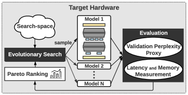
Figure 1: High-level overview of LTS. We propose a training-free zero-cost proxy for evaluating the validation perplexity of candidate architectures. Pareto-frontier search is powered by evolutionary algorithms which use the proposed proxy along with real latency and memory measurements on the target hardware to evaluate sampled architectures.

The above phenomenon coupled with the fact that a candidate architecture’s hardware performance can be measured on the target device leads to a training-free search procedure: pick one’s favorite discrete search algorithm (e.g. evolutionary search), sample candidate architectures from the search space; count their decoder parameters as a proxy for task performance (i.e., perplexity); measure their hardware performance (e.g., latency and memory) directly on the target device; and progressively create a Pareto-frontier estimate. While we have chosen a reasonable search algorithm in this work, one can plug and play any Pareto-frontier search method such as those in [20].

Building upon these insights, Figure 1 shows a high-level overview of LTS. We design the first training-free Transformer search that is performed entirely on the target (constrained) platform. As such, LTS easily performs a multi-objective NAS where several underlying hardware performance metrics, e.g., latency and peak memory utilization, are simultaneously optimized. Using our training-free proxy, we extract the $3$-dimensional Pareto-frontier of perplexity versus latency and memory in a record-breaking time of $<3$ hours on a commodity Intel Core i7 CPU. Notably, LTS eliminates the carbon footprint from hundreds of GPU hours of training associated with legacy NAS methods.

To corroborate the effectiveness of our proxy, we train over $2900$ Transformers on three large language modeling benchmark datasets, namely, WikiText-103 [27], One Billion Word [7], and Pile [17]. We use LTS to search for Pareto-optimal architectural hyperparameters in two popularly used autoregressive Transformer backbones, namely, Transformer-XL [10] and GPT-2 [32]. We believe decoder parameter count should be regarded as a competitive baseline for evaluating Transformer NAS, both in terms of ranking capabilities and easy computation. We open-source our code along with tabular information of our trained models to foster future NAS research on Transformers.

2 Related Work

Here, we discuss literature on automated search for Transformer architectures in the language domain. We refer to extensive surveys on NAS [14, 49] for a broader overview of the field.

Decoder-only Architectures. So et al. [37] search over TensorFlow programs that implement an autoregressive language model via evolutionary search. Since most random sequences of programs either have errors or underperform, the search has to be seeded with the regular Transformer architecture, termed “Primer”. As opposed to “Primer” which uses large computation to search a general space, we aim to efficiently search the “backbone” of traditional decoder-only Transformers. Additionally, the objective in “Primer” is to find models that train faster. Our objective for NAS, however, is to deliver Pareto-frontiers for inference, with respect to perplexity and hardware constraints.

Encoder-only Architectures. Relative to decoder-only autoregressive language models, encoder-only architectures like BERT [11] have received much more recent attention from the NAS community. NAS-BERT [50] trains a supernet to efficiently search for masked language models (MLMs) which are compressed versions of the standard BERT, Such models can then be used in downstream tasks as is standard practice. Similar to NAS-BERT, Xu et al. [51] train a supernet to conduct architecture search with the aim of finding more efficient BERT variants. They find interesting empirical insights into supernet training issues like differing gradients at the same node from different child architectures and different tensors as input and output at every node in the supernet. The authors propose fixes that significantly improve supernet training. Tsai et al. [41], Yin et al. [53], Gao et al. [16] also conduct variants of supernet training with the aim of finding more efficient BERT models.

Encoder-Decoder Related: Applying the well-known DARTS [24] approach to Transformer search spaces leads to memory-hungry supernets. To mitigate this issue, Zhao et al. [61] propose a multi-split reversible network and a memory-efficient backpropagation algorithm. One of the earliest papers that applied discrete NAS to Transformer search spaces was [36], which uses a modified form of evolutionary search. Due to the expense of directly performing discrete search on the search space, this work incurs extremely large computation overhead. Follow-up work by [46] uses the Once-For-All [6] approach to train a supernet for encoder-decoder architectures used in machine translation. Search is performed on subsamples of the supernet that inherit weights to estimate task accuracy. For each target device, the authors train a small neural network regressor on thousands of architectures to estimate latency. As opposed to using a latency estimator, LTS evaluates the latency of each candidate architecture on the target hardware. Notably, by performing the search directly on the target platform, LTS can easily incorporate various hardware performance metrics, e.g., peak memory utilization, for which accurate estimators may not exist. To the best of our knowledge, such holistic integration of multiple hardware metrics in Transformer NAS has not been explored previously.

3 Lightweight Transformer Search

We perform an evolutionary search over candidate architectures to extract models that lie on the Pareto-frontier. In contrast to the vast majority of prior methods that deliver a single architecture from the search space, our search is performed over the entire Pareto, generating architectures with a wide range of latency, peak memory utilization, and perplexity with one round of search. This alleviates the need to repeat the NAS algorithm for each hardware performance constraint.

To evaluate candidate models during the search, LTS uses a training-free proxy for the validation perplexity. By incorporating training-free evaluation metrics, LTS, for the first time, performs the entire search directly on the target (constrained) hardware. Therefore, we can use real measurements of hardware performance during the search. Algorithm 1 outlines the iterative process

Input: Search space $\mathcal{D}$, $n_{iter}$

Output: Perplexity-latency-memory Pareto-frontier $\mathbb{F}$

1 $\mathcal{L},\mathcal{M},\mathcal{P},\mathbb{F}\leftarrow\emptyset,\emptyset,\emptyset,\emptyset$

2 while $N\leq n_{iter}$ do

3       $\mathbb{F}^{\prime}\leftarrow$ Subsample($\mathbb{F}$)

4       $\mathbb{S}_{N}\leftarrow EA(\mathbb{F}^{\prime},\mathcal{D})$

       // hardware profiling

5       $\mathcal{L}\leftarrow\mathcal{L}\bigcup$ Latency($\mathbb{S}_{N}$)

6       $\mathcal{M}\leftarrow\mathcal{M}\bigcup$ Memory($\mathbb{S}_{N}$)

       // estimate perplexity

7       $\mathcal{P}\leftarrow\mathcal{P}\bigcup$ Proxy($\mathbb{S}_{N}$)

       // update the Pareto-frontier

8       $\mathbb{F}\leftarrow$ LowerConvexHull($\mathcal{P},\mathcal{L},\mathcal{M}$)

Algorithm 1 LTS’s training-free NAS

performed in LTS for finding candidate architectures in the search space ($\mathcal{D}$), that lie on the $3$-dimensional Pareto-frontier ($\mathbb{F}$) of perplexity versus latency and memory. At each iteration, a set of points ($\mathbb{F^{\prime}}$) are subsampled from the current Pareto-frontier. A new batch of architectures ($\mathbb{S}_{N}$) are then sampled from $\mathbb{F^{\prime}}$ using evolutionary algorithms ($EA(.)$). The new samples are evaluated in terms of latency ($\mathcal{L}$), peak memory utilization ($\mathcal{M}$), and validation perplexity ($\mathcal{P}$). Latency and memory are measured directly on the target hardware while the perplexity is indirectly estimated using our accurate and training-free proxy methods. Finally, the Pareto-frontier is recalibrated using the lower convex hull of all sampled architectures. In the context of multi-objective NAS, Pareto-frontier points are those where no single metric (e.g., perplexity, latency, and memory) can be improved without degrading at least one other metric [20]. To satisfy application-specific needs, optional upper bounds can be placed on the latency and/or memory of sampled architectures during search.

Search Space. Figure 2 shows all elastic parameters in LTS search space, namely, number of layers (n_layer), number of attention heads (n_head), decoder output dimension (d_model), inner dimension of the feed forward network (d_inner), embedding dimension (d_embed), and the division factor ($k$) of adaptive embedding [3]. These architectural parameters are compatible with popularly used autoregressive

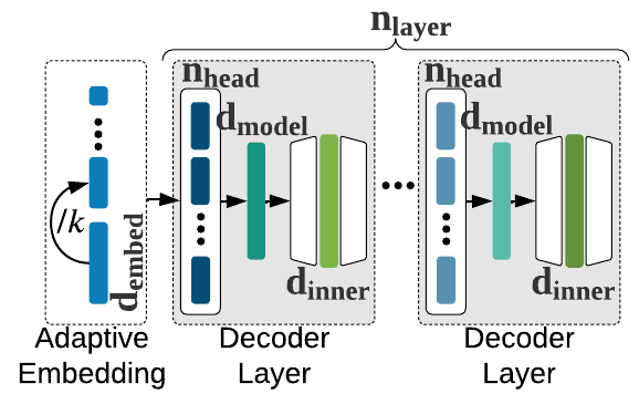
Figure 2: Elastic parameters in LTS search space.

Transformer backbones, e.g., GPT. For preliminaries on autoregressive Transformers, please see Appendix A. We adopt a heterogeneous search space where the backbone parameters are decided on a per-layer basis. This is in contrast to the homogeneous structure commonly used in Transformers [10, 5], which reuses the same configuration for all layers. Compared to homogeneous models, the flexibility associated with heterogeneous architectures enables them to obtain much better hardware performance under the same perplexity budget (see Section 4.4).

Heterogeneous search space was previously explored in [46]. However, due to the underlying supernet structure, not all design parameters can change freely. As an example, the dimensionality of the Q, K, V vectors inside the encoder and decoder layers is fixed to a large value of $512$ to accommodate inheritance from the supernet. Our search space, however, allows exploration of all internal dimensions without constraints. By not relying on the supernet structure, our search space easily encapsulates various Transformer backbones with different configurations of the input/output embedding layers and elastic internal dimensions.

LTS searches over the following values for the architectural parameters in our backbones: n_layer$\in\{2,\dots,16|1\}$, d_model$\in\{128,\dots,1024|64\}$, d_inner$\in\{256,\dots,4096|64\}$, and n_head$\in\{2,4,8\}$. Additionally we explore adaptive input embedding [3] with d_embed$\in\{128,256,512\}$ and factor $k\in\{1,2,4\}$. Once a d_model is sampled, we adjust the lower bound of the above range for d_inner to $2\times$d_model. Encoding this heuristic inside the search ensures that the acquired models will not suffer from training collapse. Our heterogeneous search space encapsulates more than $10^{54}$ different architectures. Such high dimensionality further validates the critical need for training-free NAS.

3.1 Training-free Architecture Ranking

$\blacktriangleright$ Low-cost Ranking Proxies. Recently, Abdelfattah et al. [1] utilize the summation of pruning scores over all model weights as the ranking proxy for Convolutional Neural Networks (CNNs), where a higher score corresponds to higher architecture rank in the search space. White et al. [48] analyze these and more recent proxies and find that no particular proxy performs consistently well over various tasks and baselines, while parameter and floating point operations (FLOPS) count proxies are quite competitive. However, they did not include Transformer-based search spaces in their analysis. To the best of our knowledge, low-cost (pruning-based) proxies have not been evaluated on Transformer search spaces in the language domain. Note that one cannot naively apply these proxies to language models. Specifically, since the embedding layer in Transformers is equivalent to a lookup operation, special care must be taken to omit this layer from the proxy computation. Using this insight, we perform the first systematic study of low-cost proxies for NAS on autoregressive Transformers for text prediction.

We leverage various pruning metrics, namely, grad_norm , snip  [23], grasp  [45], fisher  [40], and synflow  [38]. We also study jacob_cov  [26] and relu_log_det  [25] which are low-cost scoring mechanisms proposed for NAS on CNNs in vision tasks. While these low-cost techniques do not perform model training, they require forward and backward passes over the architecture to compute the proxy, which can be time-consuming on low-end hardware. Additionally, the aforesaid pruning techniques, by definition, incorporate the final softmax projection layer in their score assessment. Such an approach seems reasonable for CNNs dealing with a few classification labels, however, it can skew the evaluation for autoregressive Transformers dealing with a large output vocabulary space. To overcome these shortcomings, we introduce a zero-cost architecture ranking strategy in the next section that outperforms the proposed low-cost proxies in terms of ranking precision, is data free, and does not perform any forward/backward propagation.

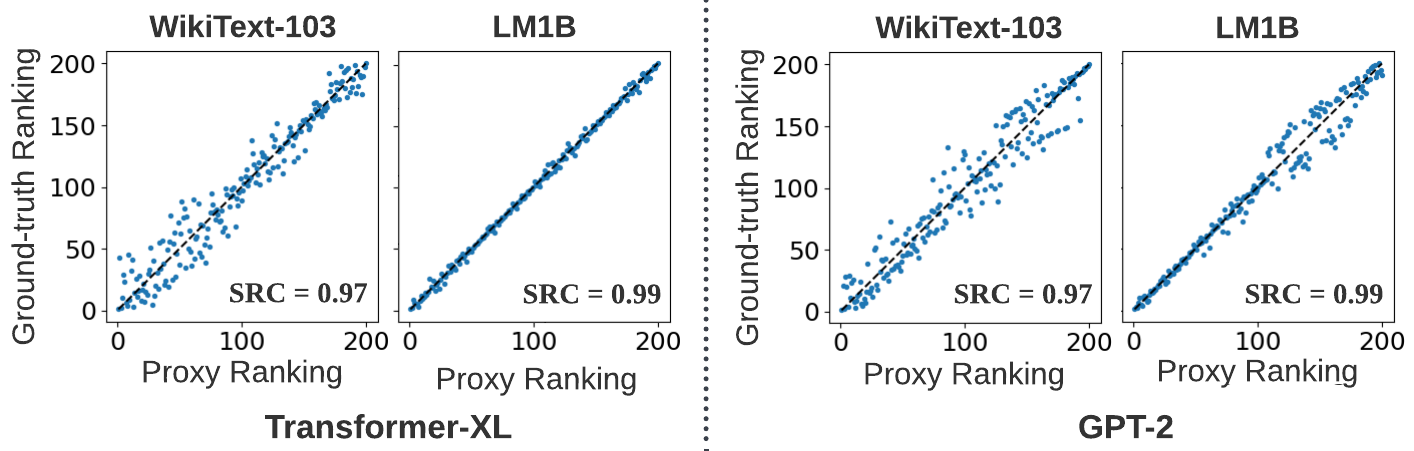
Figure 3: Our training-free zero-cost proxy based on decoder parameter count is highly correlated with the (ground truth) validation perplexity after full training. Each plot contains $200$ architectures sampled randomly from the search space of Transformer-XL or GPT-2 backbone.

$\blacktriangleright$ Decoder Parameter Count as a Proxy. We empirically establish a strong correlation between the parameter count of decoder layers and final model performance in terms of validation perplexity. We evaluate $200$ architectures sampled uniformly at random from the search space of two autoregressive Transformer backbones, namely, Transformer-XL and GPT-2. These architectures are trained fully on WikiText-103 and One Billion Word (LM1B) datasets, which consumes over $\mathbf{25000}$ GPU-hours on NVIDIA A100 and V100 nodes. We compare the ranking obtained using decoder parameter count proxy and the ground truth ranking after full training in Figure 3. On WikiText-103, zero-cost ranking using the decoder parameter count obtains a Spearman’s Rank Correlation (SRC) of $0.97$ with full training. SRC further increases to $0.99$ for the more complex LM1B benchmark on both backbones. This validates that the decoder parameter count is strongly correlated with final model performance, thereby providing a reliable training-free proxy for NAS.

4 Experiments

We conduct experiments to seek answers to the following critical questions:

How well can training-free proxies perform compared to training-based methods for estimating the performance of Transformer models?

How does model topology affect the performance of the proposed decoder parameter proxy?

Can our training-free decoder parameter count proxy be integrated inside a search algorithm to estimate the Pareto-frontier? How accurate is such an estimation of the Pareto?

Which models are on the Pareto-frontier of perplexity, latency, and memory for different hardware?

How well do LTS models perform in zero and one-shot settings compared to hand-designed variants when evaluated on downstream tasks?

We empirically answer questions , , , and in Sections 4.2, 4.3, 4.4, and 4.5 respectively. We further address question in Appendix C where we show the Pareto-frontier models extracted by the decoder parameter count proxy are very close to the ground truth Pareto-frontier with an average of $0.6\%$ perplexity difference. Additionally, we show the efficacy of the decoder parameter count proxy when performing search on different ranges of model sizes in Appendix C, Figure 12.

4.1 Experimental Setup

Please refer to Appendix B for information about the benchmarked datasets, along with details of our training and evaluation setup, hyperparameter optimization, and evolutionary search algorithm.

Backbones. We apply our search on two widely used autoregressive Transformer backbones, namely, Transformer-XL [10] and GPT-2 [32] that are trained from scratch with varying architectural hyperparameters. The internal structure of these backbones are quite similar, containing decoder blocks with attention and feed-forward layers. The difference between the backbones lies mainly in their dataflow structure; the Transformer-XL backbone adopts a recurrence methodology over past states coupled with relative positional encoding which enables modeling longer term dependencies.

Performance Criteria. To evaluate the ranking performance of various proxies, we first establish a ground truth ranking of candidate architectures by training them until full convergence. This ground truth ranking is then utilized to compute two performance criteria as follows:

$\blacktriangleright$ Common Ratio (CR): We define CR as the percentage overlap between the ground truth ranking of architectures versus the ranking obtained from the proxy. CR quantifies the ability of the proxy ranking to identify the top$k\%$ architectures based on their validation perplexity after full training.

$\blacktriangleright$ Spearman’s Rank Correlation (SRC): We use this metric to measure the correlation between the proxy ranking and the ground truth. Ideally, the proxy ranking should have high correlation with the ground truth over the entire search space as well as high-performing candidate models.

4.2 How do training-free proxies perform compared to training-based methods?

In this section, we benchmark several proxy methods for estimating the rank of candidate architectures. Specifically, we investigate three different ranking techniques, namely, partial training, low-cost methods, and number of decoder parameters.

$\blacktriangleright$ Partial Training. We first analyze the relationship between validation perplexity after a shortened training period versus that of full training for ranking candidate models. We stop the training after $\tau\in[1.25\%,87.5\%]$ of the total training iterations needed for model convergence. Figure 4 demonstrates the SRC and CR of partial training with various $\tau$s, evaluated on $100$ randomly selected models from the Transformer-XL backbone, trained on WikiText-103. The horizontal axis denotes the average time required for $\tau$ iterations of training across all sampled models. Intuitively, a higher number of training iterations results in a more accurate estimate of the final perplexity. Nevertheless, the increased wall-clock time prohibits training during search and also imposes the need for GPUs. Interestingly, very few training iterations, i.e., $1.25\%$, provide a very good proxy for final performance with an SRC of $>0.9$ on the entire population. Our training-free proxy, i.e., decoder parameter count, also shows competitive SRC compared to partial training.

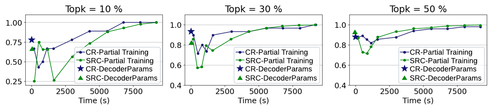
Figure 4: Comparison between partial training and our zero-cost proxy, i.e., decoder parameter count, in terms of ranking performance and timing overhead. Each subplot corresponds to a top$k\%$ of the randomly sampled models, based on their validation perplexity after full training.

$\blacktriangleright$ Low-cost Proxies. We benchmark various low-cost methods introduced in Section 3.1 on $200$ randomly sampled architectures from the Transformer-XL backbone, trained on WikiText-103. Figure 5 shows the SRC between low-cost proxies and the ground truth ranking after full training.

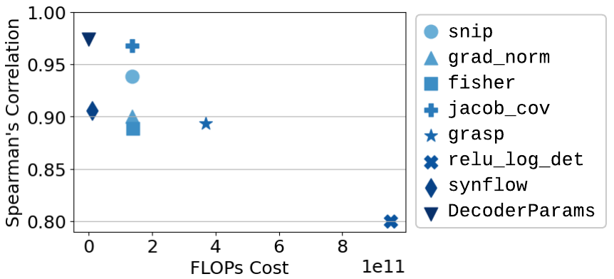
Figure 5: SRC between low-cost proxies and the ground truth ranking after full training of 200 randomly sampled Transformers. The decoder parameter count obtains the best SRC with zero cost.

We measure the cost of each proxy in terms of FLOPs. As seen, the evaluated low-cost proxies have a strong correlation with the ground truth ranking (even the lowest performing relu_log_det has $>0.8$ SRC), validating the effectiveness of training-free NAS on autoregressive Transformers. The lower performance of relu_log_det can be attributed to the much higher frequency of ReLU activations in CNNs, for which the method was originally developed, compared to Transformer-based architectures. Our analysis of randomly selected models with homogeneous structures also shows a strong correlation between the low-cost proxies and validation perplexity, with decoder parameter count outperforming other proxies (see Appendix D).

$\blacktriangleright$ Parameter Count. Figure 6a demonstrates the final validation perplexity versus the total number of model parameters for $200$ randomly sampled architectures from GPT-2 and Transformer-XL backbones. This figure contains two important observations: (1) the validation perplexity has a downward trend as the number of parameters increases, (2) The discontinuity is caused by the dominance of embedding parameters when moving to the small Transformer regime. We highlight several example points in Figure 6a where the architectures are nearly identical but the adaptive input embedding factor $k$ is changed. Changing $k\in\{1,2,4\}$ (shown with different colors in Figure 6a) varies the total parameter count without much influence on the validation perplexity.

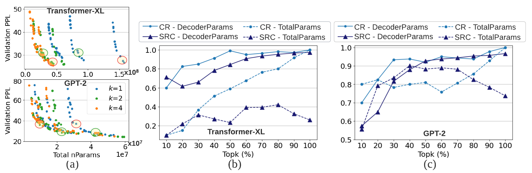
Figure 6: (a) Validation perplexity after full training versus total parameters for $200$ randomly sampled architectures trained on WikiText-103. The clear downward trend suggests a strong correlation between parameter count and perplexity. (b), (c) Performance of parameter count proxies for ranking the randomly sampled architectures with Transformer-XL and GPT-2 backbones.

The above observations motivate us to evaluate two proxies, i.e., total number of parameters and decoder parameter count. Figures 6b and 6c demonstrate the CR and SRC metrics evaluated on the $200$ randomly sampled models divided into top$k\%$ bins based on their validation perplexity. As shown, the total number of parameters generally has a lower SRC with the validation perplexity, compared to decoder parameter count. This is due to the masking effect of embedding parameters, particularly in the Transformer-XL backbone. The total number of decoder parameters, however, provides a highly accurate, zero-cost proxy with an SRC of $0.97$ with the perplexity over all models, after full training. We further show the high correlation between decoder parameter count and validation perplexity for Transformer architectures with homogeneous decoder blocks in the supplementary material, Appendix D. While our main focus is on autoregressive, decoder-only, Transformers, we provide preliminary results on the ranking performance of parameter count proxies for encoder-only and encoder-decoder Transformers in Appendix J.

4.3 How does variation in model topology affect decoder parameter count as a proxy?

The low-cost proxies introduced in Section 3.1, rely on forward and backward passes through the network. As such, they automatically capture the topology of the underlying architecture via the dataflow. The decoder parameter count proxy, however, is topology-agnostic. In this section, we investigate the effect of topology on the performance of decoder parameter count proxy. Specifically, we seek to answer whether for a given decoder parameter count budget, the aspect ratio of the architecture, i.e., trading off the width versus the depth, can affect the final validation perplexity.

We define the aspect ratio of the architecture as d_model (=width), divided by n_layer (=depth). This metric provides a sense of how skewed the topology is and has been used in prior works which study scaling laws for language models [22]. For a given decoder parameter count budget, we generate several random architectures from the GPT-2 backbone with a wide range of the width-to-depth aspect ratios. The generated models span wide, shallow topologies (e.g., d_model=$1256$, n_layer=$2$) to narrow, deep topologies (e.g., d_model=$112$, n_layer=$100$). Figure 7(a) shows the validation perplexity of said architectures after full training on WikiText-103 versus their aspect ratio. The maximum deviation (from the median) of the validation perplexity is $<12.8\%$ for a given decoder parameter count, across a wide range of aspect ratios $\in[1,630]$. Our findings on the heterogeneous search space complement the empirical results by [22] where decoder parameter count largely determines perplexity for homogeneous Transformer architectures, irrespective of shape (see Figure 5 in [22]).

We observe stable training when scaling models from the GPT-2 backbone up to $100$ layers, with the perplexity increasing only when the aspect ratio nears $1$. Nevertheless, such deep models are not part of our search space as they have high latency and are unsuitable for lightweight inference. For the purposes of hardware-aware and efficient Transformer NAS, decoder parameter count proxy holds a very high correlation with validation perplexity, regardless of the architecture topology as shown in Figure 7(a). We further validate the effect of topology on decoder parameter count proxy for the Transformer-XL backbone in Figure 14 of Appendix E. Our results demonstrate less than $7\%$ deviation (from the median) in validation perplexity for different aspect ratios $\in[8,323]$.

Note that while models with the same parameter count have very similar validation perplexities, the topology in fact affects their hardware performance, i.e., latency (up to $2.8\times$) and peak memory utilization (up to $5.5\times$), as shown in Figures 7(b) and 7(c). This motivates the need for incorporating hardware metrics in NAS to find the best topology.

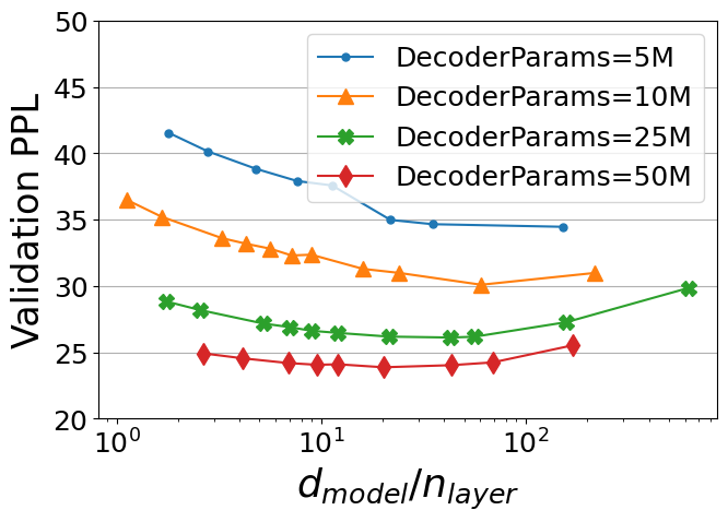
(a)

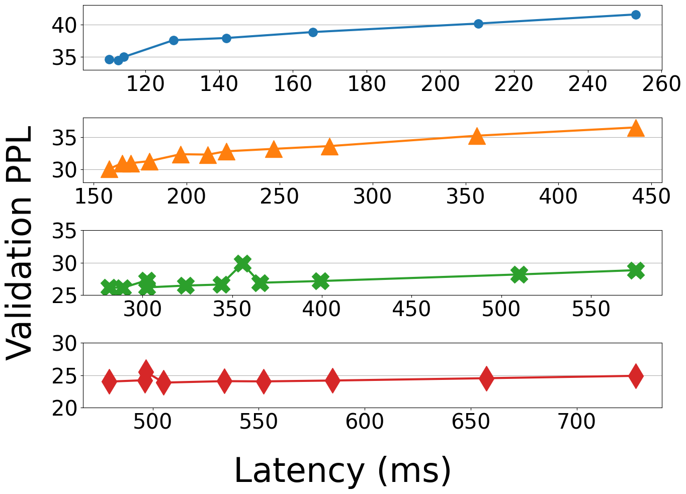
(b)

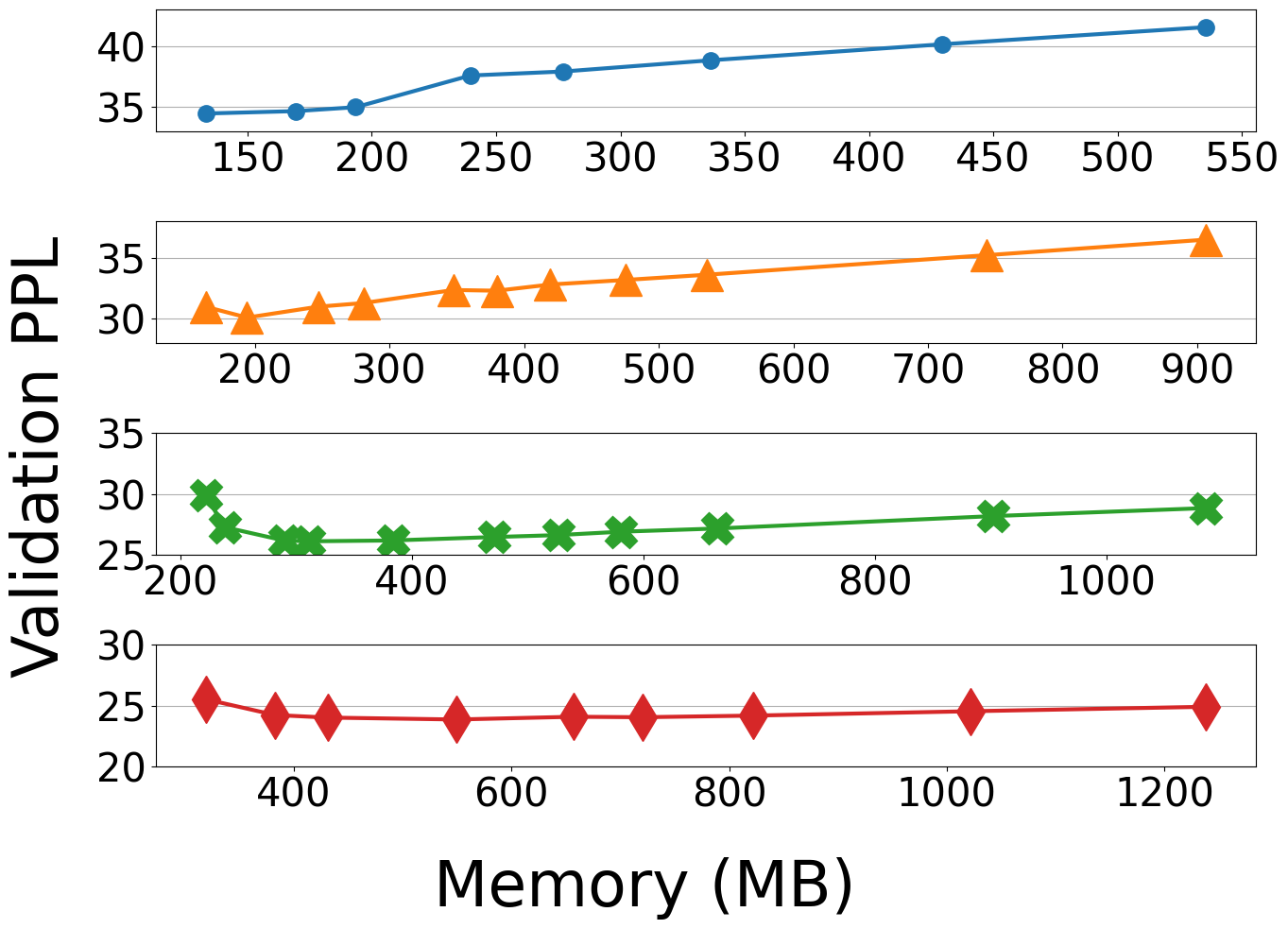
(c)

Figure 7: Validation perplexity after full training versus the (a) width-to-depth aspect ratio, (b) latency, and (c) peak memory utilization. Models are randomly generated from the GPT-2 backbone and trained on WikiText-103. For a given decoder parameter count, we observe low variation in perplexity across different models, regardless of their topology. The topology, however, significantly affects the latency (up to $2.8\times$) and peak memory utilization (up to $5.5\times$) for models with the same perplexity.

4.4 Pareto-frontier models for various hardware platforms

We run LTS on different target hardware and obtain a range of Pareto-optimal architectures with various latency/memory/perplexity characteristics. During search, we fix the adaptive input embedding factor to $k=4$ to search models that are lightweight while ensuring nearly on-par validation perplexity with non-adaptive input embedding. As the baseline Pareto, we benchmark the Transformer-XL (base) and GPT-2 (small) models with homogeneous layers $\in[1,16]$. This is because the straightforward way to produce architectures of different latency/memory is varying the number of layers (layer-scaling) [42, 10]. We compare our NAS-generated architectures with layer-scaled backbones and achieve better validation perplexity and/or lower latency and peak memory utilization. All baseline and NAS-generated models are trained using the same setup enclosed in Table 2 of Appendix B.

Figure 8 shows the Pareto-frontier architectures found by LTS versus the layer-scaled baseline. Here, all models are trained on the LM1B dataset (See Figure 16 in Appendix G for results on WikiText-103). Note that the Pareto-frontier search is performed in a $3$-dimensional space, an example of which is enclosed in Appendix F, Figure 15. For better visualization, in Figure 8 we plot $2$-dimensional slices of the Pareto-frontier with validation perplexity on the y-axis and one hardware performance metric (either latency or memory) on the x-axis.

As seen, in the low-latency regime, LTS consistently finds models that have significantly lower perplexity compared to naive scaling of the baseline Transformer-XL or GPT-2. On the Transformer-XL backbone, LTS finds architectures with an average of $19.8\%$ and $28.8\%$ lower latency and memory, while achieving similar perplexity compared to the baseline on ARM CPU. Specifically, the perplexity of the $16$-layer Transformer-XL base can be replicated on the ARM device with a lightweight model that is $1.6\times$ faster and utilizes $1.9\times$ less memory during execution. On the Corei7 CPU, the Pareto-frontier models found by LTS are on average $25.8\%$ faster and consume $30.0\%$ less memory under the same validation perplexity constraint. In this setting, LTS finds a model that replicates the perplexity of the $16$-layer Transformer-XL base while achieving $1.7\times$ faster runtime and $1.9\times$ less peak memory utilization. The savings are even higher on the GPU device, where the NAS-generated models achieve the same perplexity as the baseline with average $30.5\%$ lower latency and $27.0\%$ less memory. Specifically, an LTS model with the same perplexity as the $16$-layer Transformer-XL base has $2.5\times$ lower latency and consumes $2.0\times$ less peak memory on TITAN Xp.

On the GPT-2 backbone, NAS-generated models consume on average $11.8\%$ less memory while achieving the same validation perplexity and latency on an ARM CPU. The benefits are larger on Corei7 and TitanXP where the latency savings are $13.8\%$ and $11.9\%$, respectively. The peak memory utilization also decreases by $9.7\%$ and $12.9\%$, on average, compared to the baseline GPT-2s on Corei7 and TITAN Xp. Notably, NAS finds new architectures with the same perplexity as the $16$-layer GPT-2 with $1.3\times$, $1.5\times$ faster runtime and $1.2\times$ lower memory utilization on Corei7 and TITAN Xp.

Our heterogeneous search space allows us to find a better parameter distribution among decoder layers. Therefore, LTS delivers architectures with better performance in terms of perplexity, while reducing both latency and memory when compared to the homogeneous baselines. We provide the architecture of all baseline and LTS models shown in Figure 8 in Tables 4-7 of Appendix I.

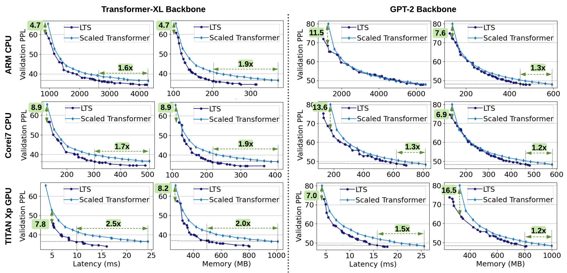
Figure 8: 2D visualization of the perplexity versus latency and memory Pareto-frontier found by LTS, versus the scaled backbone models with varying number of layers, trained on the LM1B dataset. Architectural parameters for models shown here are detailed in Appendix I.

$\blacktriangleright$ Search Efficiency. The main component in LTS search time is the latency/peak memory utilization measurement for candidate architectures since evaluating the model perplexity is instant using the decoder parameter count. Therefore, our search finishes in a few hours on commodity hardware, e.g., taking only $0.9$, $2.6$, and $17.2$ hours on a TITAN Xp GPU, Corei7 CPU, and an ARM core, respectively. To provide more context into the timing analysis, full training of even one $16$-layer Transformer-XL base model on LM1B using a machine with $8\times$ NVIDIA V100 GPUs takes $15.8$ hours. Once the Pareto-frontier models are identified, the user can pick a model based on their desired hardware constraints and fully train it on the target dataset. LTS is an alternate paradigm to that of training large supernets; our search can run directly on the target device and GPUs are only needed for training the final chosen Pareto-frontier model after search.

In Table 1 we study the ranking performance of partial training ($500$ steps) versus the decoder parameter count proxy for evaluating $1200$ architectures from the Transformer-XL backbone during LTS search. Astonishingly the decoder parameter count proxy gets higher SRC compared to partial training, while effectively removing training from the inner loop of search for NAS.

	Train Iter	GPU Hours	$CO_{2}$e (lbs)	SRC
Full Training	40,000	19,024	5433	1.0
Partial Training	500	231	66	0.92
	5,000	2690	768	0.96
# Decoder Params	0	0	$\sim$0	0.98

Table 1: Ranking abilities of full and partial training versus our proxy for $1200$ models sampled during LTS search. Training time is reported for WikiText-103 and NVIDIA V100 GPU. Decoder parameter count proxy obtains an SRC of $0.98$ using zero compute.

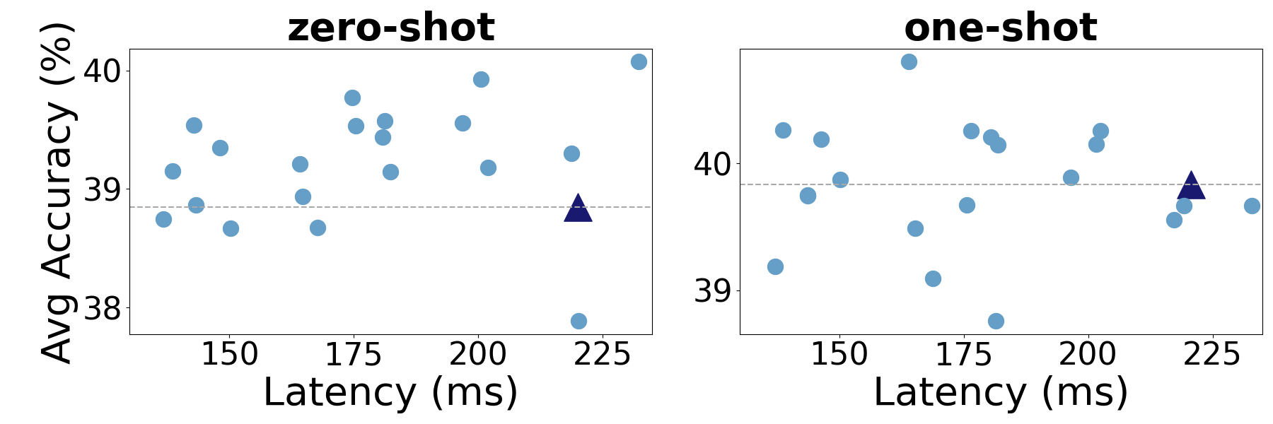
Figure 9: Average zero and one-shot accuracy obtained by LTS models (dots) and the baseline OPT-$350$M (triangle) across $14$ NLP tasks. Latency is measured on an A6000 NVIDIA GPU. Architectural parameters for all models shown here are detailed in Appendix I.

4.5 Zero and one-shot performance comparison of LTS models with OPT

Zhang et al. [58] open-source a set of pre-trained decoder-only language models, called OPT, which can be used for zero or few-shot inference on various NLP tasks. Below, we compare the performance of LTS Pareto-frontier models with the hand-designed OPT architecture in zero and one-shot settings.

We use LTS to search for language models with a GPT-2 backbone which have $300$M to $500$M total parameters to compare with the $350$M parameter OPT. Our search space is detailed in Appendix H. The search is conducted with latency as the target hardware metric and decoder parameter count as a proxy for perplexity. Once the search concludes, We train $20$ models from the Pareto-frontier along with OPT-$350$M on $28$B tokens from the Pile [17]. The pretrained models are then evaluated on $14$ downstream NLP tasks, namely, HellaSwag [57], PIQA [4], ARC (easy and challenge) [9], OpenBookQA [28], WinoGrande [34], and SuperGLUE [44] benchmarks BoolQ, CB, COPA, WIC, WSC, MultiRC, RTE, and ReCoRD. The training hyperparameters and the evaluation setup are outlined in Appendix B. Figure 9 shows the overall average accuracy obtained across all $14$ tasks versus the inference latency for LTS models and the baseline OPT. As shown, NAS-generated models achieve a higher average accuracy with lower latency compared to the hand-designed OPT-$350$M model. We provide a per-task breakdown of zero and one-shot accuracy in Appendix H, Figure 17.

$\blacktriangleright$ Zero-shot Performance. Figure 17(a) demonstrates the zero-shot accuracy obtained by LTS and OPT-$350$M on the benchmarked tasks. Compared to the OPT-$350$M architecture, LTS finds models that achieve higher accuracy and lower latency in the zero-shot setting on all evaluated downstream tasks. Specifically, the maximum achievable accuracy of our NAS-generated models is $0.2-8.6\%$ higher than OPT-$350$M with an average speedup of $1.2\times$. If latency is prioritized, LTS delivers models which are, on average, $1.5\times$ faster and up to $4.6\%$ more accurate than OPT-$350$M .

$\blacktriangleright$ One-shot Performance. Similar trends can be observed for one-shot evaluation as shown for different tasks in Figure 17(b). LTS Pareto-frontier models improve the per-task accuracy of OPT-$350$M on $12$ out of $14$ tasks by $0.1-8.0\%$, while achieving an average speedup of $1.2\times$. On the same tasks, LTS Pareto-frontier includes models that enjoy up to $1.6\times$ speedup over OPT-$350$M with an average $1.5\%$ higher accuracy. On the RTE task, the best LTS model has $0.4\%$ lower accuracy but $1.6\times$ faster runtime. On the WSC task, the best performing LTS model obtains a similar one-shot accuracy as OPT-$350$M, but with $1.5\times$ faster runtime.

5 Limitations and Future Work

Decoder parameter count provides a simple yet accurate proxy for ranking autoregressive Transformers. This should serve as a strong baseline for future works on Transformer NAS. Our focus is mainly on autoregressive, decoder-only transformers. We therefore, study perplexity as the commonly used metric for language modeling tasks. Nevertheless, recent literature on scaling laws for Transformers suggest a similar correlation between parameter count and task metrics may exist for encoder only (BERT-style) Transformers or encoder-decoder models used in neural machine translation (NMT) [19]. Additionally, recent findings [39] show specific scaling laws exist between model size and downstream task metrics, e.g., GLUE [43]. Inspired by these observations, we provide preliminary studies that suggest parameter count proxies may be applicable to Transformers in other domains. Detailed investigations of such zero-cost proxies for NAS on heterogeneous BERT-style or NMT models with new performance metrics is an important future avenue of research.

6 Acknowledgements

Professor Farinaz Koushanfar’s effort has been in parts supported by the NSF TILOS AI institute, award number CCF-2112665.

Checklist

1. For all authors…

   1. Do the main claims made in the abstract and introduction accurately reflect the paper’s contributions and scope? [Yes]

   2. Did you describe the limitations of your work? [Yes] See Sections 4.3, 5, and Appendix E

   3. Did you discuss any potential negative societal impacts of your work? [Yes] See Appendix K

   4. Have you read the ethics review guidelines and ensured that your paper conforms to them? [Yes]

2. If you are including theoretical results…

   1. Did you state the full set of assumptions of all theoretical results? [N/A]

   2. Did you include complete proofs of all theoretical results? [N/A]

3. If you ran experiments…

   1. Did you include the code, data, and instructions needed to reproduce the main experimental results (either in the supplemental material or as a URL)? [Yes] The source code for LTS is available at https://github.com/microsoft/archai/tree/neurips_lts/archai/nlp

   2. Did you specify all the training details (e.g., data splits, hyperparameters, how they were chosen)? [Yes] See Appendix B

   3. Did you report error bars (e.g., with respect to the random seed after running experiments multiple times)? [N/A]

   4. Did you include the total amount of compute and the type of resources used (e.g., type of GPUs, internal cluster, or cloud provider)? [Yes]

4. If you are using existing assets (e.g., code, data, models) or curating/releasing new assets…

   1. If your work uses existing assets, did you cite the creators? [Yes] See Appendix B

   2. Did you mention the license of the assets? [N/A] All used code are open-source and publicly available

   3. Did you include any new assets either in the supplemental material or as a URL? [Yes]

   4. Did you discuss whether and how consent was obtained from people whose data you’re using/curating? [N/A]

   5. Did you discuss whether the data you are using/curating contains personally identifiable information or offensive content? [N/A]

5. If you used crowdsourcing or conducted research with human subjects…

   1. Did you include the full text of instructions given to participants and screenshots, if applicable? [N/A]

   2. Did you describe any potential participant risks, with links to Institutional Review Board (IRB) approvals, if applicable? [N/A]

   3. Did you include the estimated hourly wage paid to participants and the total amount spent on participant compensation? [N/A]

Appendix A Preliminaries on Autoregressive Transformers

Perplexity. Perplexity is a widely used metric for evaluating the performance of autoregressive language models. This metric encapsulates how well the model can predict a word. Formally, perplexity of a language model $M$ is derived using the entropy formula as:

$$Perplexity(M)=2^{H(L,M)}=2^{-\sum_{x}L(x).log(M(x)))}$$ (1)

where $L$ represents the ground truth words. As seen, the perplexity is closely tied with the cross-entropy loss of the model, i.e., $H(L,M)$.

Parameter count. Contemporary autoregressive Transformers consist of three main components, namely, the input embedding layer, hidden layers, and the final (softmax) projection layer. The embedding layer often comprises look-up table-based modules that map the input language tokens to vectors. These vectors then enter a stack of multiple hidden layers a.k.a, the decoder blocks. Each decoder block is made up of an attention layer and a feed-forward network. Once the features are extracted by the stack of decoder blocks, the final prediction is generated by passing through the softmax projection layer. When counting the number of parameters in an autoregressive Transformer, the total parameters enclosed in the hidden layers is dubbed the decoder parameter count or equivalently, the non-embedding parameter count. These parameters are architecture-dependent and do not change based on the underlying tokenization or the vocabulary size. The embedding parameter count, however, accounts for the parameters enclosed in the input embedding layer as well as the final softmax projection layer as they are both closely tied to the word embedding and vocabulary size. We visualize an autoregressive Transformer in Figure 10, where the orange blocks contain the decoder parameters and grey blocks hold the embedding parameters.

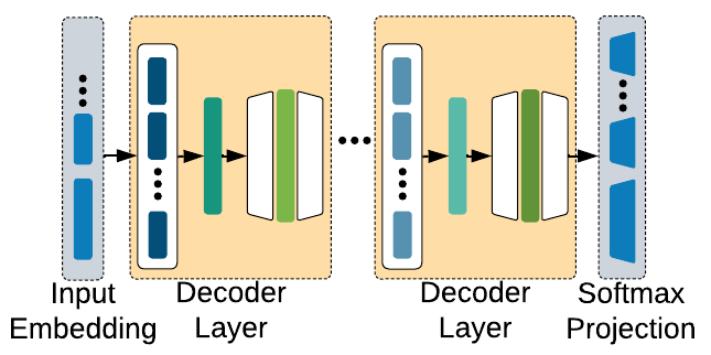
Figure 10: High-level visualization of different components in autoregressive Transformers. Here, the parameters enclosed in the orange blocks are counted as decoder parameters, while the parameters contained in the gray boxes are included in the embedding parameter count.

Appendix B Experimental Setup

Datasets. We conduct experiments on three datasets, namely, WikiText-103, LM1B, and the Pile. The datasets are tokenized using word-level and byte-pair encoding for models with Transformer-XL and GPT-2 backbones, respectively.

Training and Evaluation. We adopt the open-source code by [15] and [30] to implement the GPT-2 and Transformer-XL backbones, respectively. We further use the source code provided in [2] to implement the baseline OPT-$350$M and LTS models used in zero and one-shot evaluations. Table 2 encloses the hyperparameters used for training. In this paper, each model is trained separately from scratch. In many scenarios, the user only needs to train one model from the Pareto-frontier, which is selected based on their needs for perplexity, latency, and memory. However, if the users are interested in multiple models, they can either train all models separately or fuse them and train them simultaneously using weight sharing as in [46, 55]. As an example, if the user is interested in two particular models from the Pareto-frontier which have $3$ and $5$ layers, the user can fuse them into a single $5$-layer (super)net and train both models at the same time using weight sharing. The cost of training this supernet is roughly the same as training a $5$-layer model. Therefore, this simple trick can amortize the training cost for Pareto-frontier models.

Throughout the paper, validation perplexity is measured over a sequence length of $192$ and $32$ tokens for WikiText-103 and LM1B datasets, respectively. For our zero and one-shot evaluations, we adopt the open-source code by  Gao et al. [18]. Inference latency and peak memory utilization are measured on the target hardware for a sequence length of $192$, averaged over $10$ measurements. The sequence length is increased to $2048$ for latency comparison with the OPT baseline. We utilize PyTorch’s native benchmarking interface for measuring the latency and memory utilization of candidate architectures.

Choice of Training Hyperparameters. For each backbone, dataset, and task, we use the same training setup for all models generated by NAS. This is the common setting used in the vast majority of NAS papers, including popular benchmarks [12, 35, 56], due to the extremely high cost of NAS combined with hyperparameter optimization (HPO). The setup for our training hyperparameters is based on the evidence provided in prior art in Transformer design [22, 33, 19] and NAS [46, 62, 8]. Specifically, for the range of model sizes studied in this paper, prior work adopts the same batch size (see Table 2.1 in GPT-3 [5]), which suggests there is no significant benefit in optimizing the batch size per architecture. The original GPT-3 paper [5] also adopts the same learning rate scheduler for all models, regardless of their size. Similarly, authors of [22] show that the choice of learning rate scheduler does not have a significant effect on final model performance, which further validates that exploration of the scheduler will not alter the empirical findings in this paper.

Authors of [22] further provide a rule-of-thumb for setting the optimal learning rate (see Equation D.1 of [22]). This rule shows that changes in the optimal learning rate are negligible for the range of model sizes in our search space. We validate this by conducting an experiment that aims to find the optimal learning rate per architecture. We sweep the learning rate $\in[0.0001,0.001,0.01,0.1]$ for $100$ randomly sampled models from the GPT-2 backbone and train them on WikiText-103. The studied models span a wide range of configurations with $2-16$ layers and $2-65$M total parameters. We then pick the optimal learning rate for each architecture, i.e., the one which results in the lowest perplexity. We remeasure the correlation between newly obtained perplexities and the decoder parameter county proxy. Our learning rate optimization experiment results in two important observations: 1) for the vast majority of the architectures ($98\%$), the optimal learning rate is equal to $0.01$, i.e., the value used in all experiments (see Table 2), and 2) the ranking of architectures after convergence remains largely unchanged, leading to a correlation of $0.93$ with decoder parameter count, compared to $0.96$ when using the same learning rate for all models. The above evidence suggests that the same training setup can be used for all architectures in the search space, without affecting the results.

Table 2: LTS training hyperparameters for different backbones. Here, DO represents dropout layers.

Backbone	Dataset	Tokenizer	# Vocab	Optim.	# Steps	Batch size	LR	Scheduler	Warmup	DO	Attn DO
Transformer-XL	WT103	Word	267735	LAMB [54]	4e4	256	1e-2	Cosine	1e3	0.1	0.0
	LM1B	Word	267735	Adam	1e5	224	2.5e-4	Cosine	2e4	0.0	0.0
GPT-2	WT103	BPE	50264	LAMB [54]	4e4	256	1e-2	Cosine	1e3	0.1	0.1
	LM1B	BPE	50264	LAMB [54]	1e5	224	2.5e-4	Cosine	2e4	0.1	0.1
	Pile	BPE	50272	Adam	5.48e4	256	3e-5	Linear	715	0.1	0.0

Search Setup. Evolutionary search is performed for $30$ iterations with a population size of $100$; the parent population accounts for $20$ samples out of the total $100$; $40$ mutated samples are generated per iteration from a mutation probability of $0.3$, and $40$ samples are created using crossover.

Appendix C How Good is the Decoder Parameters Proxy for Pareto-frontier Search?

In this Section, we validate whether the decoder parameter count proxy actually helps find Pareto-frontier models which are close to the ground truth Pareto front. We first fully train all $1200$ architectures sampled from the Transformer-XL backbone during the evolutionary search (1). Using the validation perplexity obtained after full training, we rank all sampled architectures and extract the ground truth Pareto-frontier of perplexity versus latency. We train the models on the WikiText-103 dataset and benchmark Intel Xeon E5-2690 CPU as our target hardware platform for latency measurement in this experiment.

Figure 11 represents a scatter plot of the validation perplexity (after full training) versus latency for all sampled architectures during the search. The ground truth Pareto-frontier, by definition, is the lower convex hull of the dark navy dots, corresponding to models with the lowest validation perplexity for any given latency constraint. We mark the Pareto-frontier points found by the training-free proxy with orange color. As shown, the architectures that were selected as the Pareto-frontier by the proxy method are either on or very close to the ground truth Pareto-frontier.

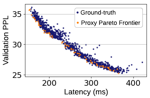
Figure 11: Perplexity versus latency Pareto obtained from full training of $1200$ architectures sampled during NAS on Transformer-XL backbone. Orange points are the Pareto-frontier extracted using decoder parameter count proxy, which lies close to the actual Pareto-frontier. Decoder parameter count holds an SRC of $0.98$ with the ground truth perplexity after full training.

We define the mean average perplexity difference as a metric to evaluate the distance ($d_{avg}$) between the proxy and ground truth Pareto-frontier:

$$d_{avg}=\frac{1}{N}\sum_{i=1}^{N}\frac{|p_{i}-p_{gt,i}|}{p_{gt,i}}$$ (2)

Here, $p_{i}$ denotes the $i$-th point on the proxy Pareto front and $p_{gt,i}$ is the closest point, in terms of latency, to $p_{i}$ on the ground truth Pareto front. The mean average perplexity difference for Figure 11 is $d_{avg}=0.6\%$. This small difference validates the effectiveness of our zero-cost proxy in correctly ranking the sampled architectures and estimating the true Pareto-frontier. In addition to the small distance between the prxoy-estimated Pareto-frontier and the ground truth, our zero-cost proxy holds a high SRC of $0.98$ over the entire Pareto, i.e., all $1200$ sampled architectures.

We further study the decoder parameter proxy in scenarios where the range of model sizes provided for search is limited. We categorize the total $1200$ sampled architectures into different bins based on the decoder parameters. Figure 12 demonstrates the SRC between the decoder parameter count proxy and the validation perplexity after full training for different model sizes. The proposed proxy provides a highly accurate ranking of candidate architectures even when exploring a small range of model sizes.

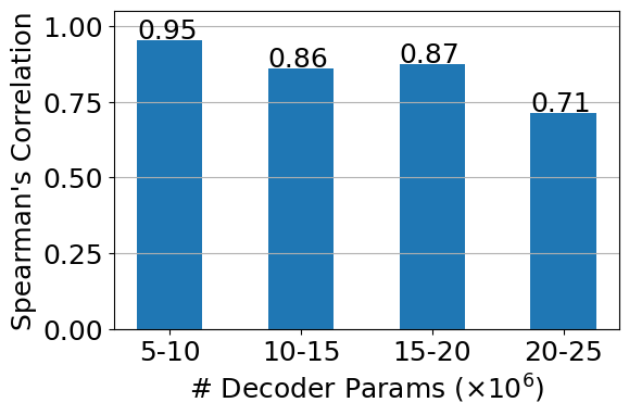
Figure 12: SRC between the decoder parameter count proxy and validation perplexity. Results are gathered on $1200$ models grouped into four bins based on their decoder parameter count. Our proxy performs well even when exploring within a small range of model sizes.

Appendix D Analysis on Homogeneous Models

In this section, we evaluate the efficacy of the proposed proxies on the homogeneous search space, i.e., when all decoder layers have the same parameter configuration. In this scenario, the parameters are sampled from the valid ranges in Section 3 to construct one decoder block. This block is then replicated based on the selected n_layer to create the Transformer architecture. In what follows, we provide experimental results gathered on $100$ randomly sampled Transformer models from the Transformer-XL backbone with homogeneous decoder blocks, trained on WikiText-103.

$\blacktriangleright$ Low-cost Proxies. Figure 13(a) demonstrates the SRC between various low-cost methods and the validation perplexity after full training. On the horizontal axis, we report the total computation required for each proxy in terms of FLOPs. Commensurate with the findings on the heterogeneous models, we observe a strong correlation between the low-cost proxies and validation perplexity, with the decoder parameter count outperforming other proxies. Note that we omit the relu_log_det method from Figure 13(a) as it provides a low SRC of $0.42$ due to heavy reliance on ReLU activations.

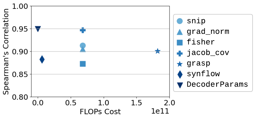
(a)

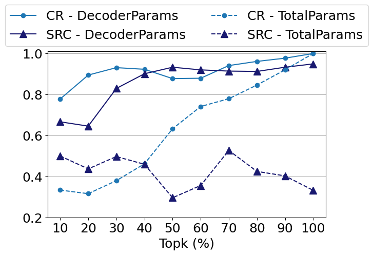
(b)

Figure 13: Experiments conducted on $100$ randomly sampled Transformers with homogeneous decoder blocks, trained on WikiText-103. (a) SRC between the ranking obtained from low-cost proxies and the ground truth ranking after full training. The decoder parameter count obtains the best SRC with zero cost. (b) Performance of parameter count proxies. The decoder parameter count provides a very accurate ranking proxy with an SRC of $0.95$ over all models.

$\blacktriangleright$ Parameter Count. As seen in Figure 13(b), the total parameter count has a low SRC with the validation perplexity while the decoder parameter count provides an accurate proxy with an SRC of $0.95$ over all architectures. These findings on the homogeneous search space are well-aligned with the observations in the heterogeneous space.

Appendix E How Does Model Topology Affect the Training-free Proxies?

Figure 14(a) shows the validation perplexity versus the aspect ratio of random architectures sampled from the Transformer-XL backbone and trained on WikiText-103. Here, the models span wide, shallow topologies (e.g., d_model=$1024$, n_layer=$3$) to narrow, deep topologies (e.g., d_model=$128$, n_layer=$35$). The maximum change in the validation perplexity for a given decoder parameter count is $<7\%$ for a wide range of aspect ratios $\in[8,323]$. Nevertheless, for the same decoder parameter count budget, the latency and peak memory utilization vary by $1.3\times$ and $2.0\times$ as shown in Figures 14(b) and 14(c).

For deeper architectures (more than $40$ layers) with the Transformer-XL backbone, we observe an increase in the validation perplexity, which results in a deviation from the pattern in Figure 14a. This observation is associated with the inherent difficulty in training deeper architectures, which can be mitigated with the proposed techniques in the literature [47]. Nevertheless, such deep models have a high latency, which makes them unsuitable for lightweight inference. For hardware-aware and efficient Transformer NAS, our search space contains architectures with less than $16$ layers. In this scenario, the decoder parameter count proxy holds a very high correlation with validation perplexity, regardless of the architecture topology as shown in Figure 14(a).

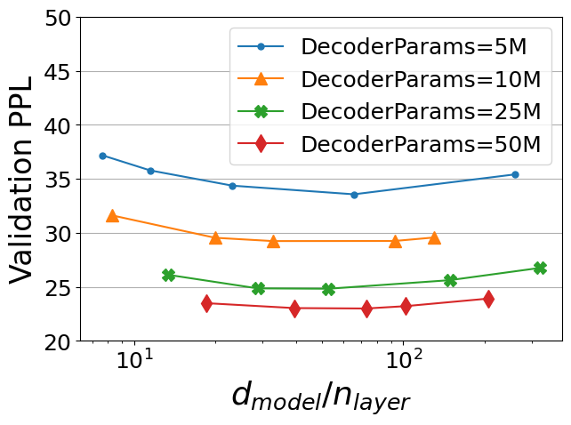
(a)

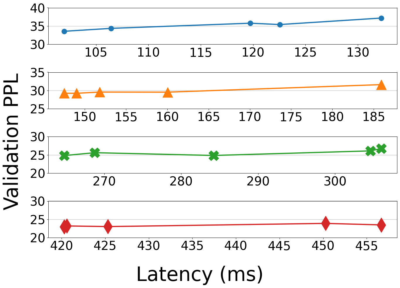
(b)

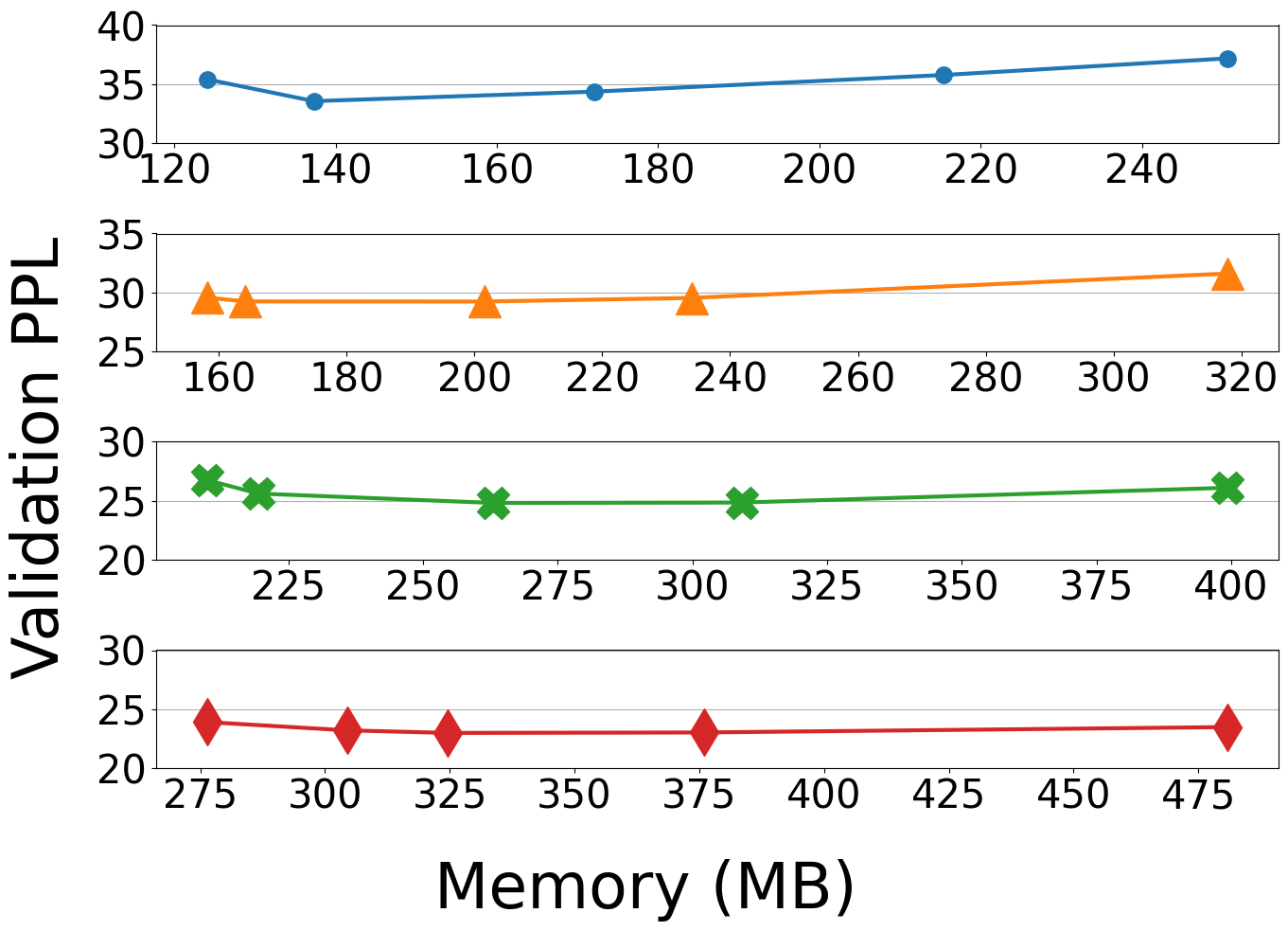
(c)

Figure 14: Validation perplexity after full training versus (a) the width-to-depth aspect ratio, (b) latency, and (c) peak memory utilization. Models are randomly generated from the Transformer-XL backbone and trained on WikiText-103. For a given decoder parameter count, we observe low variation in perplexity across different models, regardless of their topology. The topology, however, significantly affects the latency and peak memory utilization for models with the same perplexity.

Appendix F 3D Pareto Visualization

Figure 15 visualizes the $3$-dimensional Pareto obtained during search on the GPT-2 backbone. Here, the black and blue points denote regular and Pareto-frontier architectures, respectively. The pair of red dots are architectures which match in both memory and decoder parameter count ($\sim$ perplexity). However, as shown, their latency differs by $2\times$. The pair of green points correspond to models with the same decoder parameter count ($\sim$ perplexity) and latency, while the memory still differs by $30$MB, which is non-negligible for memory-constrained application. In a $2$-objective Pareto-frontier search of perplexity versus memory (or latency), each pair of red (or green) dots will result in similar evaluations. While in reality, they have very different characteristics in terms of the overlooked metric. This experiment validates the need for multi-objective Pareto-frontier search, which simultaneously takes into account multiple hardware performance metrics.

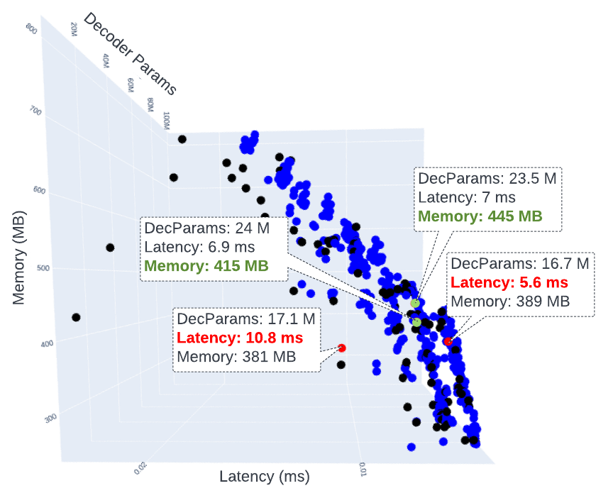
Figure 15: 3D visualization of our multi-objective NAS for the GPT-2 backbone on TITAN Xp GPU. Architectures with similar memory and decoder parameter count can result in drastically different runtimes (up to $2\times$ difference). Similarly, architectures with similar decoder parameter count and latency may have different peak memory utilization. Therefore, it is important to perform multi-objective NAS where several hardware characteristics are simultaneously taken into account when extracting the Pareto-frontier.

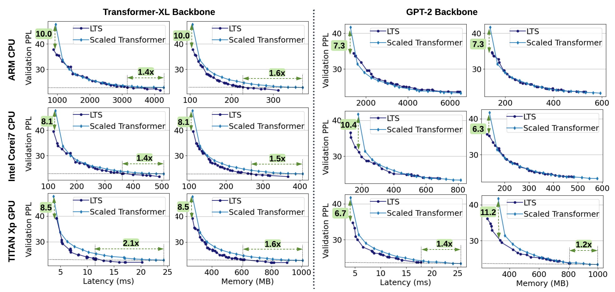
Figure 16: 2D visualization of the perplexity versus latency and memory Pareto-frontier found by LTS and scaled backbone models with varying number of layers. All models are trained on the WikiText-103 dataset. The architectural parameters for all models are enclosed in Appendix I.

Appendix G LTS Pareto-frontier on WikiText-103

We compare the Pareto-frontier architectures found by LTS with the baseline after full training on the WikiText-103 dataset in Figure 16. Commensurate with the findings on the LM1B dataset, the NAS-generated models outperform the baselines in at least one of the three metrics, i.e., perplexity, latency, and peak memory utilization. We note that the gap between the baseline models and those obtained from NAS is larger when training on the LM1B dataset. This is due to the challenging nature of LM1B, which exceeds the WikiText-103 dataset size by $\sim 10\times$. Thus, it is harder for hand-crafted baseline models to compete with the optimized LTS architectures on LM1B.

On the Transformer-XL backbone, the models on LTS Pareto-frontier for the ARM CPU have, on average, $3.8\%$ faster runtime and $20.7\%$ less memory under the same validation perplexity budget. On the Corei7, the runtime and memory savings increase to $13.2\%$ and $19.6\%$, respectively, while matching the baseline perplexity. We achieve our highest benefits on TITAN Xp GPU where LTS Pareto-frontier models have, on average, $31.8\%$ lower latency and $21.5\%$ lower memory utilization. Notably, the validation perplexity of the baseline $16$-layer Transformer-XL base can be achieved with a lightweight model with $2.1\times$ lower latency while consuming $1.6\times$ less memory at runtime.

On the GPT-2 backbone, LTS achieves $6.3-11.2$ lower perplexity in the low-latency-and-memory regime. As we transition to larger models and higher latency, our results show that the GPT-2 architecture is nearly optimal on WikiText-103 when performing inference on a CPU. The benefits are more significant when targeting a GPU; For any given perplexity achieved by the baseline, LTS Pareto-frontier on TITAN Xp delivers, on average, $9.0\%$ lower latency and $4.5\%$ lower memory. Therefore, the perplexity and memory of the baseline $16$-layer GPT-2 can be achieved by a new model that runs $1.4\times$ faster and consumes $1.2\times$ less memory on TITAN Xp.

Appendix H Zero and One-Shot Evaluation of LTS Models

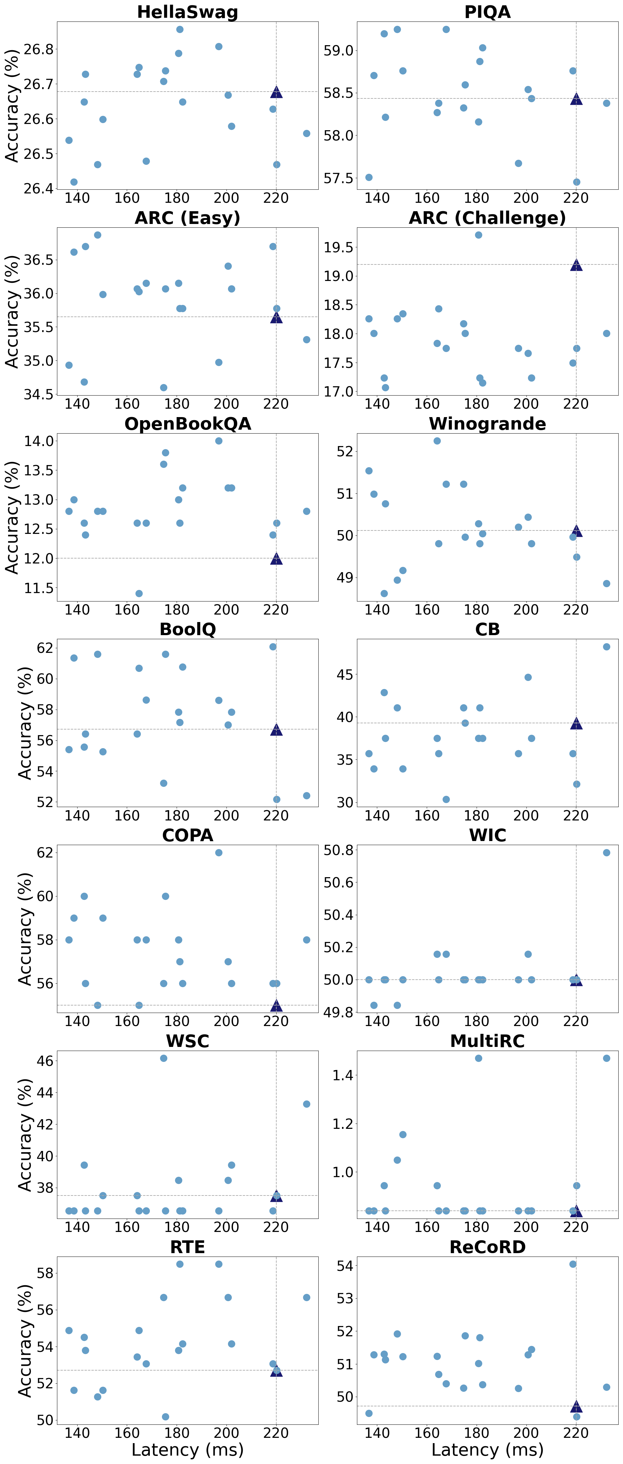
(a) zero-shot

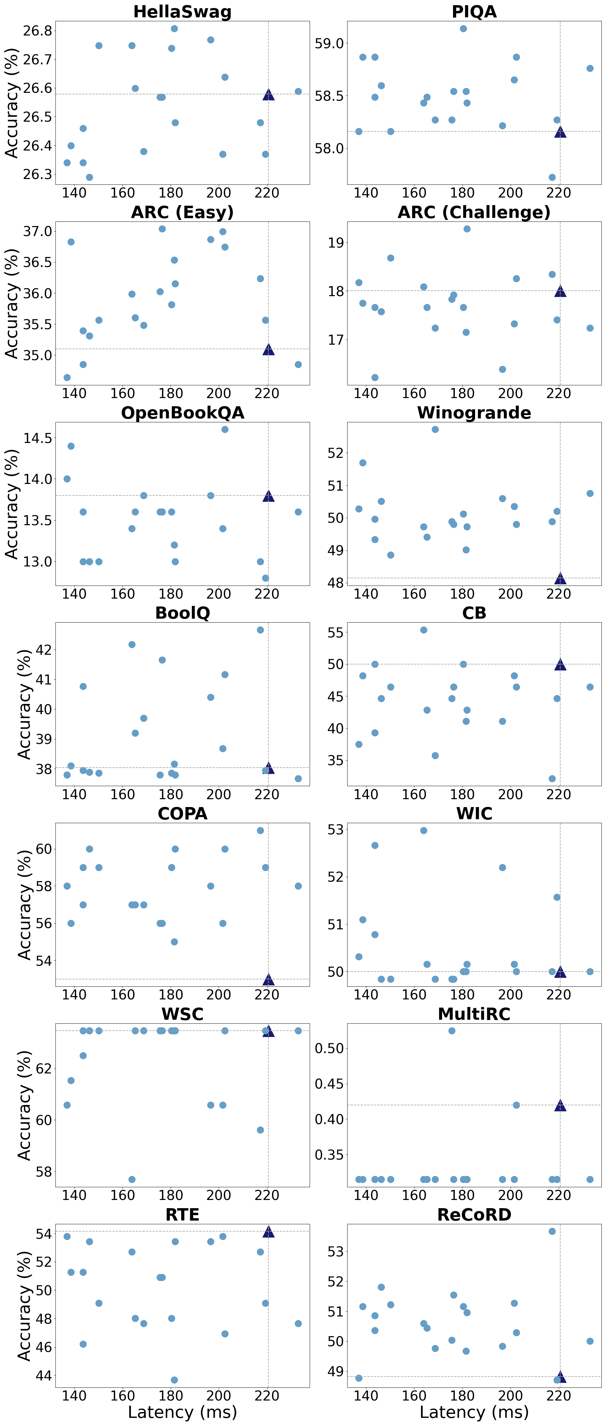
(b) one-shot

Figure 17: LTS Pareto-frontier models (dots) achieve a higher zero and one-shot accuracy with lower latency compared to the hand-designed OPT-$350$M model (triangle). Latency is measured on an A6000 NVIDIA GPU. Architectural parameters for all models shown here are detailed in Appendix I.

For this experiment, we design our search space to cover models with a similar parameter count budget as the OPT-$350$M model. To this end, we search over the following values for the architectural parameters: n_layer$\in\{3,\dots,29|1\}$, d_model$\in\{512,\dots,1472|64\}$, d_inner$\in\{512,\dots,6080|64\}$, and n_head$\in\{2,4,8,16\}$. To directly compare with OPT, we use a generic, non-adaptive embedding layer for our models. Therefore, the search space does not include the $k$ factor and d_embed=d_model.

Figures 17(a) and 17(b) show the per-task zero and one-shot performance of LTS models and OPT-$350$M. Please refer to Section 4.5 of the main paper for a summarization of the results in these figures.

Appendix I Architecture Details

Tables 4, 5, 6, 7 enclose the architecture parameters for the baseline and NAS-generated models in Figures 8 and 16 for Transformer-XL and GPT-2 backbones. Table 3 further holds the architecture details of models used in our zero and one-shot evaluations of Figures 9 and 17. For each target hardware, the rows of the table are ordered based on increasing decoder parameter count (decreasing validation perplexity). For all models, d_head=d_model/n_head and d_embed=d_model. For models in Tables 4, 5, 6, 7, the adaptive input embedding factor is set to $k=4$. The models in Table 3, however, use the generic, non-adaptive, input embedding ($k=1$) following the original OPT architecture [58].

Appendix J Transformers in other Domains

In what follows, we perform preliminary experiments on Transformers used on other domains to investigate the applicability of parameter-based proxies for ranking.

Encoder-only Transformers. BERT [11] is a widely popular Transformer composed of encoder blocks, which is used in a variety of tasks, e.g., question answering and language inference. The main difference between BERT and the Transformers studied in this paper is the usage of bidirectional versus causal attention. Specifically, the encoder blocks in BERT are trained to compute attention between each input token and all surrounding tokens. In autoregressive models, however, attention is only computed for tokens appearing prior to the current token. BERT is trained with a mixture of masked language modeling and next sentence prediction objectives to ensure applicability to language modeling as well as downstream language understanding tasks. We use the architectural parameters described in Section 3 to construct the search space and randomly sample $300$ models from the BERT backbone. We then train all models on WikiText-103 for 40K steps following the training setup provided in the original BERT paper [11] for the batch size, sequence length, optimizer, learning rate, vocabulary size, and tokenizer. Figure 18 demonstrates the CR and SRC of encoder parameter count and test perplexity measured on various top$k\%$ performing BERT models. As seen, both the encoder and total parameter count provide a highly accurate proxy for test perplexity of BERT, achieving an SRC of $0.96$ and $0.98$, respectively. This trend suggests that parameter-based proxies for NAS can be applicable to encoder-only search spaces as well.

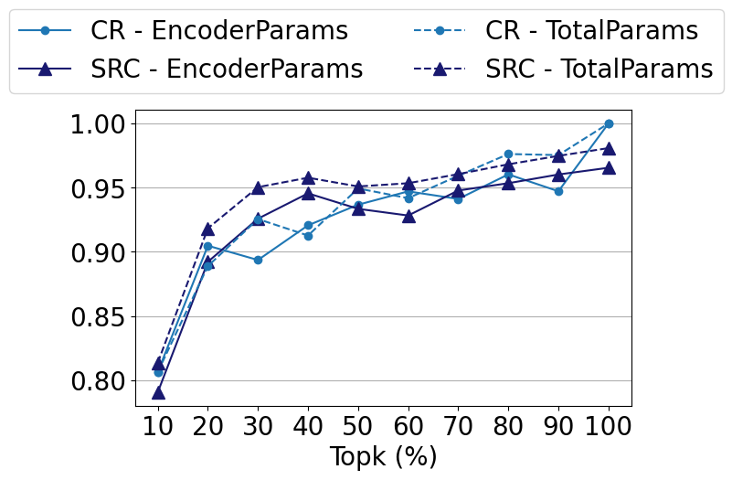
Figure 18: Performance of parameter count proxies on $300$ randomly sampled models from the BERT backbone, trained on WikiText-103. Both encoder and total parameter counts provide a very accurate ranking proxy with an SRC of 0.96 and 0.98 over all models, respectively.

Encoder-Decoder Transformers. Transformers in this domain comprise both encoder and decoder layers with bidirectional and causal attention computation. This unique structure makes these models suitable for sequence-to-sequence tasks such as Neural Machine Translation (NMT). Recent work [19] shows that the performance of encoder-decoder Transformers also follows a scaling law with model size. This power-law behavior between model size and performance can be leveraged to develop training-free proxies for ranking these architectures during search. We test our hypothesis by performing experiments on the open-source NMT benchmark by [60, 59] which consists of $2000$ Transformers trained on various language pairs. The pre-trained Transformers in this benchmark have homogeneous layers, i.e., the architectural parameters are the same for all layers and identical for the encoder and the decoder. In addition to architectural parameters, the search space for this benchmark also includes various BPE tokenization and learning rates. We, therefore, pre-process the benchmark by gathering all instances of Transformers for a fixed BPE. Then for each given architecture, we keep the results corresponding to the best-performing learning rate.

Figure 19 shows a heatmap of the SRC between parameter count proxies and perplexity as well as the BLEU score. As seen, the ranking performance of total parameter count versus non-embedding parameter count, i.e., parameters enclosed in the encoder and decoder blocks, is largely similar. On certain tasks, e.g., ‘ja-en’, ‘so-en’, and ‘sw-en’ the parameter count proxies perform quite well, achieving a high SRC with both the BLEU score and perplexity. Interestingly, on ‘so-en’ and ‘sw-en’, the parameter count and performance are inversely correlated, which may be due to the limited training data for these language pairs which gives smaller models a leading advantage over larger architectures. While these preliminary results show promise for parameter-based proxies in NAS for NMT, several aspects require further investigation, e.g., the effect of architectural heterogeneity and dataset size on the performance of these proxies. Studying these aspects may perhaps lead to a new formulation of training-free proxies for NMT and are out of scope for this paper.

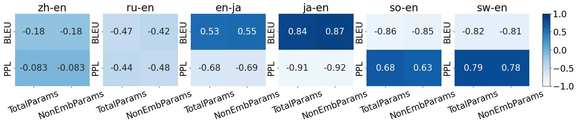
Figure 19: SRC between parameter count proxies and performance metrics, i.e., BLEU score and perplexity (PPL) for translation between various language pairs. The “NonEmbParams” label denotes the parameters enclosed in the encoder and decoder blocks while the “TotalParams” label corresponds to the total parameter count including those in the embedding layers. Here, darker versus lighter colors show a high positive and negative correlation, respectively.

Appendix K Ethics Statement and Broader Impact

We provide an extremely lightweight method for NAS on autoregressive Transformers. Our work is likely to increase the adoption of NAS in the NLP domain, providing several prevalent benefits:

Firstly, more widespread adoption of automated techniques, e.g., NAS eliminates the need for laborious trials and error for manual design of Transformer architectures, freeing up hundreds of hours of man-power as well as computational resources. Secondly, automating architecture design can trigger the generation of new models with superior performance, which benefits the ever-growing applications of NLP in the everyday life. Finally, by making the search algorithm efficient, we ensure it can be accessible to the general scientific public without need for any expensive mode training, thereby minimizing the unwanted byproducts of the Deep Learning era such as the carbon footprint, and power consumption. While the benefits of automation in NLP are plenty, it can lead to potential side effects that have not been yet fully unveiled. Since our work advances the use of NAS in the NLP design pipeline, there is need for scrutiny of the models which have been automatically designed with respect to aspects such as bias, misinformation, and nefarious activity, to name a few.

Table 3: Detailed architectural parameters for all models in Figure 9 with GPT-2 backbone.

	nlayer	dmodel	nhead	dinner	DecoderParams (M)
baseline (OPT-$350$M)	24	1024	16	4096	304.4
M1	26	1024	16	2816	261.4
M2	15	1280	16	4480	273.2
M3	24	1280	8	1856	274.3
M4	16	1344	8	3840	283.8
M5	14	1344	8	4800	284.8
M6	20	1216	4	3456	289.2
M7	16	1344	16	4096	294.8
M8	28	1344	8	1344	306.6
M9	28	1088	8	2816	306.7
M10	26	1152	16	2816	309.4
M11	25	832	2	5760	310.9
M12	20	1280	16	3456	310.9
M13	19	1280	8	3840	314.2
M14	26	1152	4	3008	320.9
M15	19	1472	8	2816	325.5
M16	13	1472	4	5568	329.0
M17	14	1480	2	5824	367.3
M18	20	1152	8	5760	374.3
M19	26	1024	4	5696	414.8
M20	25	1408	8	3136	422.3

Table 4: Detailed architectural parameters for all models in Figure 8 with Transformer-XL backbone.

		nlayer	dmodel	nhead	dinner	DecoderParams (M)
baseline		$\in$[1,16]	512	8	2048	-
ARM	M1	2	512	[2, 2]	[1216, 1280]	5.2
	M2	3	320	[2, 4, 2]	[1472, 2368, 3392]	6.2
	M3	2	512	[2, 2]	[2560, 2176]	7.5
	M4	2	512	[2, 2]	[3904, 1792]	8.5
	M5	2	640	[2, 2]	[3520, 3456]	13.0
	M6	2	704	[8, 2]	[3904, 3968]	16.1
	M7	2	832	[2, 2]	[3264, 3968]	19.0
	M8	2	960	[2, 2]	[3648, 3968]	23.9
	M9	2	960	[2, 2]	[3904, 3968]	24.4
	M10	3	960	[2, 2, 2]	[1856, 2368, 3392]	28.5
	M11	3	832	[2, 2, 2]	[3904, 3968, 3008]	28.5
	M12	3	960	[2, 4, 2]	[3328, 2368, 3200]	30.9
	M13	3	960	[4, 2, 2]	[3648, 3584, 3584]	34.6
	M14	3	960	[2, 2, 2]	[3904, 3584, 3456]	34.9
	M15	3	960	[2, 2, 8]	[4032, 3968, 3904]	36.7
	M16	4	896	[4, 2, 8, 2]	[3904, 3008, 3520, 3584]	41.2
	M17	4	960	[8, 8, 8, 4]	[4032, 3968, 2880, 3200]	45.5
	M18	4	960	[2, 2, 2, 2]	[3840, 3904, 3520, 3072]	46.0
	M19	4	960	[2, 2, 2, 2]	[4032, 3648, 3136, 4032]	47.0
	M20	4	960	[8, 2, 4, 8]	[4032, 3584, 3840, 3584]	47.4
	M21	4	960	[2, 2, 4, 2]	[3904, 3968, 3840, 3584]	47.8
	M22	5	960	[2, 2, 2, 2, 2]	[3904, 3968, 3264, 3456, 3200]	57.3
	M23	5	960	[2, 2, 2, 8, 2]	[3904, 3648, 3136, 3648, 3840]	58.0
	M24	6	960	[2, 2, 2, 2, 2, 8]	[3328, 2624, 3392, 2944, 3008, 3904]	64.6
	M25	6	960	[2, 2, 4, 2, 8, 8]	[3584, 2624, 3392, 3968, 3008, 3328]	65.9
	M26	6	960	[2, 4, 2, 2, 2, 2]	[2112, 3840, 3328, 3264, 3968, 3648]	66.4
	M27	6	960	[2, 4, 2, 2, 8, 2]	[3904, 3008, 3392, 3648, 3392, 3584]	67.9
	M28	6	960	[2, 2, 2, 2, 2, 4]	[3968, 3968, 3456, 3456, 3776, 2432]	68.1
	M29	6	960	[2, 4, 8, 4, 2, 8]	[3904, 3008, 3392, 3200, 3968, 3904]	68.8
	M30	6	960	[8, 8, 2, 4, 2, 4]	[3904, 3648, 3136, 3648, 3200, 3840]	68.8
	M31	6	960	[8, 4, 8, 4, 2, 8]	[3904, 3648, 3392, 3200, 3968, 3840]	69.9
	M32	8	896	[4, 2, 2, 4, 4, 2, 4, 8]	[3584, 3968, 3392, 3904, 2240, 1856, 2560, 3264]	76.6
	M33	8	896	[4, 2, 2, 2, 4, 4, 4, 2]	[3584, 3584, 3520, 2368, 2752, 4032, 3520, 3264]	79.9
	M34	9	896	[4, 2, 4, 4, 8, 2, 8, 8, 2]	[3840, 3136, 3520, 2880, 3200, 3008, 3328, 2560, 3136]	87.5
	M35	8	960	[2, 4, 4, 4, 4, 8, 2, 2]	[3968, 3584, 3520, 3072, 3968, 4032, 1856, 3712]	90.2
	M36	12	832	[2, 4, 4, 2, 2, 8, 8, 8, 4, 4, 2, 8]	[3136, 2112, 2112, 2368, 2752, 2432, 2432, 2176, 3456, 3712, 2880, 3712]	97.0
	M37	9	960	[4, 4, 8, 2, 2, 2, 8, 8, 2]	[2112, 3008, 3520, 3648, 3968, 4032, 1984, 3200, 3520]	97.2
	M38	9	960	[8, 2, 4, 2, 8, 8, 8, 2, 2]	[3968, 3008, 3520, 3200, 3200, 4032, 1984, 2816, 3520]	97.7
	M39	12	832	[4, 4, 4, 2, 2, 8, 4, 8, 2, 8, 2, 8]	[3136, 3968, 2112, 2368, 3072, 2240, 2624, 2112, 3456, 3072, 2880, 3264]	98.7
Corei7	M1	2	384	[2, 2]	[896, 2816]	4.3
	M2	2	576	[2, 2]	[1792, 2816]	8.6
	M3	2	576	[2, 2]	[1408, 3776]	9.3
	M4	2	832	[2, 2]	[1728, 1536]	12.4
	M5	2	768	[2, 2]	[3776, 1920]	14.7
	M6	2	768	[2, 2]	[2112, 3584]	14.7
	M7	2	832	[2, 2]	[3776, 3392]	18.9
	M8	2	832	[2, 2]	[3968, 3584]	19.5
	M9	2	960	[2, 4]	[1984, 3840]	20.4
	M10	2	960	[8, 8]	[3968, 3584]	23.7
	M11	2	960	[2, 2]	[3904, 3904]	24.2
	M12	3	896	[2, 2, 2]	[2304, 3904, 3904]	30.2
	M13	3	960	[2, 2, 4]	[2176, 3840, 2880]	30.9
	M14	3	960	[2, 2, 4]	[3776, 2880, 3904]	34.1
	M15	3	960	[2, 8, 2]	[3840, 3840, 3904]	36.1
	M16	3	960	[2, 8, 8]	[3904, 3840, 3904]	36.2
	M17	3	960	[2, 2, 8]	[3968, 3904, 3904]	36.5
	M18	4	960	[2, 4, 2, 2]	[3904, 2112, 4032, 3584]	44.6
	M19	4	960	[2, 2, 2, 4]	[2112, 3840, 3904, 3904]	44.9
	M20	4	960	[2, 4, 8, 4]	[3776, 3392, 3520, 3904]	46.5
	M21	4	960	[2, 2, 2, 4]	[3904, 3776, 3904, 3904]	48.2
	M22	5	960	[2, 2, 2, 2, 2]	[3776, 1984, 3904, 3904, 3456]	55.8
	M23	5	960	[2, 4, 2, 4, 2]	[3968, 3584, 3520, 3904, 3200]	58.0
	M24	5	960	[2, 4, 4, 4, 2]	[3776, 3840, 3904, 3904, 3968]	60.3
	M25	6	960	[2, 4, 4, 2, 2, 4]	[3776, 3840, 3904, 3904, 3008, 2304]	67.5
	M26	6	960	[2, 4, 2, 4, 2, 4]	[3776, 2112, 4032, 3584, 3200, 4032]	67.5
	M27	6	960	[2, 4, 2, 4, 4, 4]	[3776, 3840, 3904, 4032, 3648, 2432]	69.2
	M28	6	960	[4, 2, 8, 4, 2, 2]	[3840, 3712, 3520, 4032, 3200, 4032]	70.6
	M29	7	960	[2, 2, 8, 4, 2, 2, 4]	[3776, 3840, 3904, 1856, 3072, 3648, 4032]	78.7
	M30	8	960	[2, 2, 2, 4, 2, 4, 8, 2]	[3392, 1792, 3904, 3904, 3200, 2432, 1792, 2496]	80.9
	M31	8	960	[2, 2, 4, 4, 2, 4, 8, 2]	[3776, 3008, 4032, 3904, 3520, 3136, 1984, 3648]	88.8
	M32	8	960	[8, 2, 2, 4, 8, 4, 4, 8]	[3776, 3008, 3904, 3904, 2176, 4032, 4032, 3648]	91.6
	M33	13	768	[2, 8, 2, 4, 2, 2, 4, 2, 2, 8, 8, 8, 4]	[3776, 2112, 1600, 3904, 3840, 2880, 2304, 3200, 2048, 2944, 2816, 3328, 3968]	97.9
	M34	9	960	[4, 2, 4, 4, 4, 4, 8, 8, 2]	[3840, 3136, 3520, 4032, 3200, 4032, 3648, 2112, 2368]	98.9
	M35	9	960	[8, 2, 8, 8, 2, 4, 8, 2, 2]	[3520, 3008, 2880, 4032, 3200, 2432, 4032, 3904, 3136]	99.4

Table 5: Detailed architectural parameters for all models in Figure 8 with Transformer-XL backbone.

		nlayer	dmodel	nhead	dinner	DecoderParams (M)
baseline		$\in$[1,16]	512	8	2048	-
TITAN Xp	M1	2	384	[2, 2]	[1152, 2432]	4.2
	M2	2	448	[8, 2]	[2944, 3008]	7.4
	M3	2	576	[2, 2]	[2048, 1728]	7.7
	M4	2	512	[2, 2]	[2368, 3072]	8.2
	M5	2	832	[8, 2]	[3264, 3072]	17.5
	M6	2	768	[2, 2]	[3968, 4032]	18.2
	M7	2	896	[8, 4]	[4032, 2880]	20.4
	M8	2	960	[4, 8]	[3968, 3008]	22.6
	M9	2	960	[4, 8]	[3968, 3648]	23.9
	M10	2	960	[2, 2]	[3840, 3968]	24.2
	M11	3	896	[8, 4, 8]	[4032, 2112, 3392]	29.2
	M12	3	896	[2, 2, 2]	[3840, 2880, 3840]	31.0
	M13	3	960	[2, 2, 2]	[3584, 3072, 2624]	31.7
	M14	3	960	[4, 2, 2]	[3840, 3008, 3840]	34.4
	M15	3	960	[8, 2, 8]	[4032, 4032, 3520]	36.1
	M16	3	960	[2, 2, 8]	[3584, 4032, 4032]	36.2
	M17	3	960	[2, 2, 8]	[4032, 4032, 3840]	36.7
	M18	3	960	[8, 4, 8]	[4032, 4032, 4032]	37.1
	M19	4	896	[4, 4, 8, 8]	[4032, 3456, 3328, 3392]	41.6
	M20	4	960	[4, 2, 8, 8]	[3840, 3008, 3328, 3584]	44.9
	M21	4	960	[2, 2, 8, 8]	[4032, 3968, 3904, 3840]	48.7
	M22	4	960	[4, 2, 4, 4]	[3840, 4032, 3904, 4032]	48.8
	M23	5	960	[4, 2, 4, 4, 8]	[3840, 3008, 3392, 2496, 4032]	55.3
	M24	5	960	[4, 2, 8, 8, 8]	[3840, 3008, 3840, 3328, 3968]	57.6
	M25	5	960	[2, 2, 4, 4, 4]	[3968, 4032, 3328, 4032, 2752]	57.9
	M26	6	896	[8, 4, 8, 4, 8, 8]	[3328, 2112, 3392, 3904, 3328, 3264]	58.8
	M27	5	960	[8, 2, 8, 8, 4]	[4032, 3008, 3840, 3904, 3968]	59.1
	M28	5	960	[2, 4, 2, 2, 8]	[3968, 3968, 3840, 4032, 3904]	60.9
	M29	6	896	[2, 2, 4, 4, 2, 2]	[3840, 3968, 3840, 3328, 3904, 3904]	65.0
	M30	6	960	[4, 8, 8, 4, 8, 4]	[3072, 3584, 3392, 3840, 3328, 3712]	67.9
	M31	6	960	[4, 8, 8, 8, 4, 4]	[3840, 3584, 3392, 3328, 3968, 3776]	69.7
	M32	6	960	[4, 8, 8, 8, 8, 2]	[3840, 3840, 3392, 3840, 3328, 3712]	69.9
	M33	6	960	[4, 2, 2, 4, 2, 8]	[3840, 3008, 3840, 3904, 4032, 3392]	70.0
	M34	6	960	[2, 4, 8, 8, 4, 2]	[3840, 3968, 3840, 3328, 4032, 3776]	71.5
	M35	7	960	[4, 8, 8, 8, 8, 2, 8]	[3840, 3968, 3840, 3328, 3968, 3328, 4032]	82.8
	M36	8	960	[4, 2, 8, 8, 8, 4, 8, 8]	[3840, 3968, 3840, 3328, 3072, 3328, 4032, 3072]	91.6
	M37	10	896	[8, 4, 8, 8, 8, 2, 8, 2, 4, 8]	[4032, 3008, 3840, 2560, 3904, 3904, 3072, 3264, 2368, 2496]	98.4
	M38	12	832	[2, 4, 8, 8, 8, 8, 8, 8, 8, 8, 4, 2]	[3840, 2816, 2112, 3584, 3648, 2432, 2304, 3008, 2880, 1664, 2432, 3776]	99.0
	M39	9	960	[8, 8, 8, 4, 4, 8, 8, 4, 2]	[2752, 3456, 2880, 3904, 2752, 3904, 4032, 3264, 3136]	99.3
	M40	10	896	[8, 8, 8, 2, 8, 2, 2, 2, 8, 2]	[3840, 3072, 3840, 2560, 3648, 3328, 3840, 3008, 2880, 3328]	100.0

Table 6: Detailed architectural parameters for all models in Figure 8 with GPT-2 backbone.

		nlayer	dmodel	nhead	dinner	DecoderParams (M)
baseline		$\in$[1,16]	1024	12	3072	-
TITAN Xp	M1	3	256	[2, 2, 2]	[3072, 3776, 3904]	6.3
	M2	2	448	[2, 2]	[3456, 3776]	8.1
	M3	2	448	[2, 4]	[4032, 3904]	8.7
	M4	3	384	[2, 2, 2]	[3072, 2176, 4032]	8.9
	M5	2	576	[2, 2]	[3456, 3584]	10.8
	M6	4	448	[2, 2, 2, 2]	[4032, 3904, 1920, 3072]	14.8
	M7	4	512	[2, 2, 4, 2]	[3904, 3136, 1280, 2624]	15.4
	M8	2	832	[8, 2]	[3456, 3584]	17.3
	M9	2	960	[2, 8]	[3456, 3648]	21.0
	M10	2	960	[2, 2]	[3968, 3584]	21.9
	M11	5	640	[2, 2, 2, 2, 2]	[4032, 2560, 2176, 2304, 3136]	26.4
	M12	3	832	[2, 8, 4]	[3840, 3840, 3776]	27.4
	M13	5	704	[2, 2, 2, 4, 4]	[2368, 3648, 1856, 3712, 3200]	30.8
	M14	3	960	[2, 2, 2]	[3584, 3648, 4032]	32.7
	M15	3	960	[2, 2, 2]	[3904, 3520, 4032]	33.1
	M16	6	640	[2, 2, 2, 2, 2, 2]	[2624, 2560, 2880, 3776, 3648, 3840]	34.6
	M17	4	896	[2, 2, 4, 2]	[4032, 3712, 3328, 3072]	38.2
	M18	5	832	[2, 2, 2, 4, 4]	[3392, 3648, 2880, 3712, 3200]	41.9
	M19	4	960	[2, 2, 4, 2]	[3904, 3136, 3328, 3776]	42.0
	M20	4	960	[8, 8, 2, 4]	[3904, 3712, 4032, 3776]	44.4
	M21	6	832	[2, 2, 4, 2, 2, 2]	[3904, 3456, 4032, 1792, 3072, 2496]	47.9
	M22	5	896	[4, 2, 2, 2, 4]	[3968, 3200, 3840, 3328, 3648]	48.3
	M23	5	960	[2, 2, 2, 2, 2]	[3904, 3264, 3328, 3776, 3392]	52.4
	M24	5	960	[2, 2, 4, 2, 2]	[3584, 3456, 3776, 2944, 4032]	52.7
	M25	5	960	[2, 8, 2, 4, 2]	[3904, 3648, 4032, 3776, 3968]	55.6
	M26	6	960	[8, 8, 2, 2, 2, 2]	[3904, 2560, 2880, 3776, 2240, 3840]	59.1
	M27	6	960	[2, 2, 2, 4, 2, 2]	[2496, 3456, 3328, 3904, 3968, 2944]	60.8
	M28	6	960	[4, 2, 4, 4, 2, 8]	[4032, 3456, 3328, 3776, 4032, 2752]	63.2
	M29	6	960	[2, 2, 2, 4, 4, 4]	[3968, 3648, 3840, 3776, 3584, 2624]	63.4
	M30	7	960	[2, 2, 2, 4, 2, 4, 2]	[3904, 2368, 4032, 3008, 3520, 2944, 2496]	68.7
	M31	7	960	[2, 2, 4, 2, 2, 2, 4]	[3072, 3648, 3520, 3584, 3136, 1984, 3584]	69.1
	M32	7	960	[4, 2, 2, 2, 8, 2, 2]	[3712, 3648, 3584, 3520, 2752, 3008, 3392]	71.2
	M33	8	960	[2, 4, 4, 2, 2, 2, 2, 2]	[3904, 2816, 3072, 1920, 3328, 3456, 2304, 2368]	74.1
	M34	8	960	[2, 2, 2, 4, 2, 2, 8, 2]	[3520, 2368, 4032, 1792, 3200, 3776, 3200, 3648]	78.6
	M35	8	960	[4, 2, 4, 4, 8, 8, 4, 2]	[3520, 3712, 3328, 3776, 3200, 2752, 3200, 2112]	78.7
	M36	8	960	[8, 4, 2, 8, 2, 2, 2, 2]	[3520, 3840, 3328, 3776, 3200, 3776, 3968, 3648]	85.4
	M37	10	960	[2, 8, 2, 4, 2, 2, 4, 2, 8, 8]	[3648, 2560, 3776, 1792, 3968, 2752, 3200, 2368, 4032, 2368]	95.5
	M38	10	960	[2, 4, 2, 2, 4, 2, 4, 2, 4, 8]	[3840, 2240, 3328, 3776, 3648, 3200, 2944, 2368, 3968, 2880]	98.8
	M39	10	960	[2, 4, 2, 2, 2, 2, 4, 2, 4, 8]	[3840, 2240, 3328, 3776, 3200, 3200, 3968, 2368, 3968, 2816]	99.8

Table 7: Detailed architectural parameters for all models in Figure 8 with GPT-2 backbone.

		nlayer	dmodel	nhead	dinner	DecoderParams (M)
baseline		$\in$[1,16]	1024	12	3072	-
ARM	M1	2	512	[2, 2]	[1920, 1920]	6.0
	M2	3	320	[8, 2, 4]	[1920, 1920, 3712]	6.1
	M3	2	576	[2, 2]	[1344, 3200]	7.9
	M4	3	384	[2, 8, 2]	[3840, 2368, 3328]	9.1
	M5	5	384	[4, 4, 2, 4, 4]	[2880, 1920, 960, 2496, 1280]	10.3
	M6	2	768	[2, 2]	[1600, 2240]	10.6
	M7	5	320	[4, 2, 2, 4, 2]	[1344, 2240, 3776, 3008, 3648]	11.0
	M8	3	768	[2, 2, 4]	[1856, 1792, 1920]	15.7
	M9	3	704	[2, 2, 2]	[3136, 2112, 1920]	16.1
	M10	2	960	[4, 2]	[3584, 2304]	18.7
	M11	6	448	[4, 4, 2, 2, 4, 2]	[3072, 2112, 4032, 2688, 1600, 3072]	19.7
	M12	3	960	[4, 4, 2]	[2368, 2560, 2048]	24.5
	M13	4	704	[4, 8, 4, 2]	[3008, 3776, 2560, 3648]	26.3
	M14	5	704	[4, 2, 4, 2, 8]	[3584, 3136, 3776, 3072, 1856]	31.7
	M15	3	960	[2, 2, 2]	[3392, 3648, 3840]	32.0
	M16	4	960	[4, 2, 8, 2]	[2048, 3328, 1984, 1856]	32.5
	M17	7	704	[2, 4, 4, 4, 8, 2, 2]	[3008, 2560, 1920, 1856, 2112, 1728, 3136]	36.9
	M18	4	960	[2, 2, 4, 8]	[3392, 3456, 2432, 2304]	37.0
	M19	5	832	[4, 4, 4, 4, 4]	[3840, 1920, 4032, 3072, 3968]	41.9
	M20	5	960	[8, 4, 2, 2, 4]	[2560, 2048, 3648, 1728, 2304]	42.1
	M21	5	960	[4, 4, 2, 2, 2]	[3072, 2240, 1984, 2176, 3520]	43.4
	M22	5	960	[2, 4, 4, 4, 2]	[2496, 3648, 3328, 3392, 2112]	47.2
	M23	6	832	[4, 2, 4, 4, 2, 4]	[2496, 3200, 1664, 3904, 3520, 3840]	47.7
	M24	6	960	[8, 2, 2, 2, 8, 4]	[2304, 3328, 3456, 1856, 1792, 2112]	50.7
	M25	5	960	[4, 8, 2, 4, 4]	[3264, 2688, 4032, 3968, 3712]	52.4
	M26	6	960	[2, 4, 4, 2, 2, 2]	[3008, 2624, 4032, 2688, 3520, 2624]	57.7
	M27	6	960	[2, 4, 4, 2, 8, 2]	[2304, 3648, 3328, 3648, 3904, 1728]	57.8
	M28	6	960	[4, 4, 2, 4, 2, 2]	[3072, 2368, 4032, 4032, 3776, 3264]	61.6
	M29	7	960	[2, 2, 2, 8, 4, 8, 4]	[3008, 2304, 1920, 1984, 3520, 2816, 3712]	62.9
	M30	7	960	[2, 4, 4, 4, 4, 2, 2]	[3200, 4032, 2048, 2624, 2112, 2752, 2880]	63.6
	M31	7	960	[2, 4, 4, 4, 4, 2, 4]	[3584, 3648, 3328, 3392, 3200, 1984, 3200]	68.8
	M32	7	960	[2, 4, 8, 8, 2, 2, 8]	[3008, 3648, 3584, 3648, 3008, 1728, 3712]	68.8
	M33	7	960	[4, 4, 2, 4, 4, 8, 4]	[3584, 3840, 3328, 3392, 3136, 2944, 2496]	69.5
	M34	8	960	[8, 2, 2, 8, 2, 2, 8, 2]	[3008, 3648, 1792, 1984, 3008, 2816, 3712, 3520]	74.7
	M35	8	960	[2, 2, 2, 2, 8, 4, 4, 2]	[3008, 2304, 1792, 3008, 3520, 2880, 3712, 3456]	75.1
	M36	8	960	[2, 2, 2, 2, 2, 2, 4, 8]	[3008, 1792, 3840, 3392, 3520, 3136, 3712, 3520]	79.4
	M37	9	960	[2, 2, 4, 4, 8, 8, 4, 2, 4]	[1664, 1792, 2240, 3904, 3648, 3264, 2176, 3712, 1856]	79.9
	M38	11	832	[8, 4, 2, 4, 4, 2, 8, 4, 4, 8, 8]	[3072, 2368, 4032, 3968, 1664, 3968, 2176, 2624, 3840, 2176, 2112]	83.8
	M39	9	960	[4, 2, 4, 8, 2, 2, 4, 2, 4]	[2496, 3648, 3328, 3392, 3648, 1728, 2880, 3520, 2368]	85.1
	M40	9	960	[4, 2, 4, 8, 4, 2, 4, 2, 4]	[3072, 2816, 4032, 2560, 3648, 1728, 3840, 3264, 3456]	87.8
	M41	10	960	[8, 2, 4, 4, 2, 2, 4, 8, 2, 4]	[3648, 1792, 2432, 1856, 3392, 2304, 3776, 2944, 3136, 3904]	93.0
	M42	10	960	[8, 2, 2, 4, 2, 2, 2, 4, 2, 2]	[3264, 2048, 3520, 3904, 3840, 3840, 2624, 3072, 3776, 2304]	98.8
	M43	12	896	[4, 4, 4, 2, 4, 2, 4, 8, 8, 2, 4, 2]	[2048, 3136, 4032, 1792, 3584, 1728, 3136, 3008, 2560, 3200, 3648, 1728]	98.9
	M44	10	960	[4, 2, 8, 4, 2, 8, 4, 4, 4, 2]	[3584, 3968, 3328, 3904, 2368, 2112, 3904, 3520, 3328, 2688]	99.8
	M45	10	960	[8, 2, 4, 4, 4, 4, 4, 2, 2, 8]	[2688, 3200, 3840, 3392, 3520, 3136, 3392, 3520, 2880, 3200]	99.9
Corei7	M1	2	384	[2, 2]	[3840, 2432]	6.0
	M2	3	320	[2, 2, 2]	[2176, 3072, 2496]	6.2
	M3	2	512	[2, 2]	[1408, 2624]	6.2
	M4	3	384	[2, 2, 2]	[3264, 3456, 3584]	9.7
	M5	2	576	[2, 2]	[3136, 3648]	10.5
	M6	3	448	[2, 2, 2]	[4032, 3648, 4032]	12.9
	M7	4	448	[2, 2, 4, 4]	[3072, 3648, 4032, 1792]	14.5
	M8	2	768	[2, 2]	[3968, 3328]	15.9
	M9	4	576	[2, 2, 2, 2]	[3072, 2752, 3456, 3136]	19.6
	M10	2	960	[2, 2]	[3840, 3264]	21.0
	M11	4	640	[2, 2, 2, 2]	[2176, 3648, 3584, 1920]	21.1
	M12	3	960	[2, 2, 2]	[2176, 3264, 2432]	26.2
	M13	4	768	[2, 2, 2, 2]	[3584, 2112, 3392, 1920]	26.4
	M14	4	768	[2, 2, 2, 2]	[3584, 2560, 3776, 1536]	27.1
	M15	4	832	[2, 2, 2, 2]	[3904, 1984, 3392, 3136]	31.8
	M16	3	960	[2, 2, 2]	[3968, 4032, 2880]	32.0
	M17	5	768	[2, 2, 4, 2, 2]	[3648, 3072, 3392, 1984, 2944]	34.9
	M18	4	960	[2, 2, 2, 2]	[3136, 1984, 3392, 2944]	36.8
	M19	4	960	[2, 2, 2, 4]	[3968, 3456, 3584, 3136]	42.0
	M20	6	768	[4, 2, 2, 4, 2, 4]	[3584, 2112, 3456, 3136, 3840, 2560]	42.9
	M21	7	768	[2, 4, 2, 4, 4, 4, 2]	[2624, 1984, 2496, 3968, 2880, 2112, 4032]	47.5
	M22	5	960	[2, 2, 4, 2, 4]	[2176, 3264, 3392, 3008, 3328]	47.6
	M23	6	960	[4, 4, 2, 4, 2, 2]	[2048, 2624, 3520, 1984, 2880, 2624]	52.3
	M24	6	960	[2, 4, 4, 4, 2, 2]	[1792, 3456, 2752, 2240, 1664, 3840]	52.4
	M25	6	960	[4, 2, 2, 2, 4, 4]	[2176, 1664, 3648, 3136, 3968, 3904]	57.7
	M26	7	960	[2, 2, 4, 4, 2, 2, 8]	[2816, 1792, 3968, 1728, 1664, 3328, 2944]	60.9
	M27	7	896	[2, 2, 4, 2, 2, 2, 2]	[3904, 3264, 3328, 3968, 1728, 2624, 4032]	63.5
	M28	7	960	[4, 2, 4, 2, 2, 2, 2]	[3584, 2560, 1792, 1920, 3968, 2112, 3968]	64.1
	M29	8	960	[2, 2, 2, 4, 2, 2, 2, 4]	[3328, 2432, 2624, 2752, 1664, 2240, 2304, 2816]	68.3
	M30	7	960	[4, 2, 4, 2, 2, 2, 2]	[3904, 2304, 2368, 3584, 3264, 2880, 3904]	68.5
	M31	8	960	[4, 2, 4, 2, 2, 4, 2, 4]	[2560, 3648, 2624, 2112, 3328, 2112, 1792, 3328]	70.9
	M32	8	960	[4, 4, 4, 2, 2, 4, 2, 4]	[2560, 2304, 2624, 4032, 2688, 2624, 3840, 2816]	74.7
	M33	9	960	[2, 4, 2, 4, 2, 4, 2, 2, 4]	[3072, 3264, 2944, 1984, 2880, 3520, 2112, 2624, 1728]	79.6
	M34	10	896	[2, 2, 4, 2, 2, 2, 2, 2, 4, 2]	[2816, 3264, 3584, 1792, 3136, 3584, 2240, 2240, 1920, 2752]	81.2
	M35	9	960	[8, 2, 2, 2, 4, 4, 2, 4, 4]	[3904, 3648, 2432, 3136, 3264, 2816, 2240, 3072, 3840]	87.7
	M36	10	960	[4, 4, 2, 2, 4, 4, 2, 4, 4, 2]	[2176, 3264, 2752, 3136, 3968, 3520, 3776, 3328, 1728, 2496]	94.9
	M37	10	960	[4, 2, 4, 2, 2, 2, 2, 4, 2, 2]	[3904, 2112, 2496, 3968, 3968, 2624, 3904, 2304, 3200, 3840]	99.0
	M38	11	960	[4, 2, 2, 4, 2, 4, 2, 2, 4, 4, 4]	[2176, 4032, 3264, 3840, 2688, 1984, 1728, 2944, 1920, 2368, 3840]	99.8

References

- Abdelfattah et al. [2020] Mohamed S Abdelfattah, Abhinav Mehrotra, Łukasz Dudziak, and Nicholas Donald Lane. Zero-cost proxies for lightweight nas. In International Conference on Learning Representations, 2020.
- [2] Meta AI. Codebase for open pre-trained transformers. https://github.com/facebookresearch/metaseq.
- Baevski and Auli [2018] Alexei Baevski and Michael Auli. Adaptive input representations for neural language modeling. In International Conference on Learning Representations, 2018.
- Bisk et al. [2020] Yonatan Bisk, Rowan Zellers, Jianfeng Gao, Yejin Choi, et al. Piqa: Reasoning about physical commonsense in natural language. In Proceedings of the AAAI conference on artificial intelligence, volume 34, pages 7432–7439, 2020.
- Brown et al. [2020] Tom B Brown, Benjamin Mann, Nick Ryder, Melanie Subbiah, Jared Kaplan, Prafulla Dhariwal, Arvind Neelakantan, Pranav Shyam, Girish Sastry, Amanda Askell, et al. Language models are few-shot learners. arXiv preprint arXiv:2005.14165, 2020.
- Cai et al. [2019] Han Cai, Chuang Gan, Tianzhe Wang, Zhekai Zhang, and Song Han. Once-for-all: Train one network and specialize it for efficient deployment. In International Conference on Learning Representations, 2019.
- Chelba et al. [2013] Ciprian Chelba, Tomas Mikolov, Mike Schuster, Qi Ge, Thorsten Brants, Phillipp Koehn, and Tony Robinson. One billion word benchmark for measuring progress in statistical language modeling. arXiv preprint arXiv:1312.3005, 2013.
- Chen et al. [2021] Minghao Chen, Houwen Peng, Jianlong Fu, and Haibin Ling. Autoformer: Searching transformers for visual recognition. In Proceedings of the IEEE/CVF International Conference on Computer Vision, pages 12270–12280, 2021.
- Clark et al. [2018] Peter Clark, Isaac Cowhey, Oren Etzioni, Tushar Khot, Ashish Sabharwal, Carissa Schoenick, and Oyvind Tafjord. Think you have solved question answering? try arc, the ai2 reasoning challenge. arXiv preprint arXiv:1803.05457, 2018.
- Dai et al. [2019] Zihang Dai, Zhilin Yang, Yiming Yang, Jaime G Carbonell, Quoc Le, and Ruslan Salakhutdinov. Transformer-xl: Attentive language models beyond a fixed-length context. In Proceedings of the 57th Annual Meeting of the Association for Computational Linguistics, pages 2978–2988, 2019.
- Devlin et al. [2019] Jacob Devlin, Ming-Wei Chang, Kenton Lee, and Kristina Toutanova. Bert: Pre-training of deep bidirectional transformers for language understanding. In NAACL-HLT (1), 2019.
- Dong and Yang [2019] Xuanyi Dong and Yi Yang. Nas-bench-201: Extending the scope of reproducible neural architecture search. In International Conference on Learning Representations, 2019.
- Elsken et al. [2019a] Thomas Elsken, Jan Hendrik Metzen, and Frank Hutter. Efficient multi-objective neural architecture search via lamarckian evolution. In International Conference on Learning Representations, 2019a.
- Elsken et al. [2019b] Thomas Elsken, Jan Hendrik Metzen, and Frank Hutter. Neural architecture search: A survey, 2019b.
- [15] Hugging Face. Openai gpt2 by hugging face. https://huggingface.co/docs/transformers/model_doc/gpt2.
- Gao et al. [2021a] Jiahui Gao, Hang Xu, Han shi, Xiaozhe Ren, Philip L. H. Yu, Xiaodan Liang, Xin Jiang, and Zhenguo Li. Autobert-zero: Evolving bert backbone from scratch, 2021a.
- Gao et al. [2020] Leo Gao, Stella Biderman, Sid Black, Laurence Golding, Travis Hoppe, Charles Foster, Jason Phang, Horace He, Anish Thite, Noa Nabeshima, et al. The pile: An 800gb dataset of diverse text for language modeling. arXiv preprint arXiv:2101.00027, 2020.
- Gao et al. [2021b] Leo Gao, Jonathan Tow, Stella Biderman, Sid Black, Anthony DiPofi, Charles Foster, Laurence Golding, Jeffrey Hsu, Kyle McDonell, Niklas Muennighoff, Jason Phang, Laria Reynolds, Eric Tang, Anish Thite, Ben Wang, Kevin Wang, and Andy Zou. A framework for few-shot language model evaluation. https://github.com/facebookresearch/metaseq, September 2021b.
- Ghorbani et al. [2021] Behrooz Ghorbani, Orhan Firat, Markus Freitag, Ankur Bapna, Maxim Krikun, Xavier Garcia, Ciprian Chelba, and Colin Cherry. Scaling laws for neural machine translation. In International Conference on Learning Representations, 2021.
- Guerrero-Viu et al. [2021] Julia Guerrero-Viu, Sven Hauns, Sergio Izquierdo, Guilherme Miotto, Simon Schrodi, Andre Biedenkapp, Thomas Elsken, Difan Deng, Marius Lindauer, and Frank Hutter. Bag of baselines for multi-objective joint neural architecture search and hyperparameter optimization. arXiv preprint arXiv:2105.01015, 2021.
- Hu et al. [2019] Hanzhang Hu, John Langford, Rich Caruana, Saurajit Mukherjee, Eric J Horvitz, and Debadeepta Dey. Efficient forward architecture search. In H. Wallach, H. Larochelle, A. Beygelzimer, F. d'Alché-Buc, E. Fox, and R. Garnett, editors, Advances in Neural Information Processing Systems, volume 32. Curran Associates, Inc., 2019. URL https://proceedings.neurips.cc/paper/2019/file/6c468ec5a41d65815de23ec1d08d7951-Paper.pdf.
- Kaplan et al. [2020] Jared Kaplan, Sam McCandlish, Tom Henighan, Tom B Brown, Benjamin Chess, Rewon Child, Scott Gray, Alec Radford, Jeffrey Wu, and Dario Amodei. Scaling laws for neural language models. arXiv preprint arXiv:2001.08361, 2020.
- Lee et al. [2019] Namhoon Lee, Thalaiyasingam Ajanthan, and Philip Torr. SNIP: SINGLE-SHOT NETWORK PRUNING BASED ON CONNECTION SENSITIVITY. In International Conference on Learning Representations, 2019. URL https://openreview.net/forum?id=B1VZqjAcYX.
- Liu et al. [2019] Hanxiao Liu, Karen Simonyan, and Yiming Yang. DARTS: Differentiable architecture search. In International Conference on Learning Representations, 2019. URL https://openreview.net/forum?id=S1eYHoC5FX.
- Mellor et al. [2021a] Joe Mellor, Jack Turner, Amos Storkey, and Elliot J Crowley. Neural architecture search without training. In International Conference on Machine Learning, pages 7588–7598. PMLR, 2021a.
- Mellor et al. [2021b] Joseph Mellor, Jack Turner, Amos Storkey, and Elliot J. Crowley. Neural architecture search without training, 2021b. URL https://openreview.net/forum?id=g4E6SAAvACo.
- Merity et al. [2016] Stephen Merity, Caiming Xiong, James Bradbury, and Richard Socher. Pointer sentinel mixture models. arXiv preprint arXiv:1609.07843, 2016.
- Mihaylov et al. [2018] Todor Mihaylov, Peter Clark, Tushar Khot, and Ashish Sabharwal. Can a suit of armor conduct electricity? a new dataset for open book question answering. arXiv preprint arXiv:1809.02789, 2018.
- Ning et al. [2021] Xuefei Ning, Changcheng Tang, Wenshuo Li, Zixuan Zhou, Shuang Liang, Huazhong Yang, and Yu Wang. Evaluating efficient performance estimators of neural architectures. Advances in Neural Information Processing Systems, 34, 2021.
- [30] NVIDIA. Transformer-xl for pytorch. https://github.com/NVIDIA/DeepLearningExamples/tree/master/PyTorch/LanguageModeling/Transformer-XL.
- Pham et al. [2018] Hieu Pham, Melody Guan, Barret Zoph, Quoc Le, and Jeff Dean. Efficient neural architecture search via parameters sharing. In International Conference on Machine Learning, pages 4095–4104. PMLR, 2018.
- Radford et al. [2019] Alec Radford, Jeffrey Wu, Rewon Child, David Luan, Dario Amodei, Ilya Sutskever, et al. Language models are unsupervised multitask learners. OpenAI blog, 1(8):9, 2019.
- Raffel et al. [2020] Colin Raffel, Noam Shazeer, Adam Roberts, Katherine Lee, Sharan Narang, Michael Matena, Yanqi Zhou, Wei Li, Peter J Liu, et al. Exploring the limits of transfer learning with a unified text-to-text transformer. J. Mach. Learn. Res., 21(140):1–67, 2020.
- Sakaguchi et al. [2021] Keisuke Sakaguchi, Ronan Le Bras, Chandra Bhagavatula, and Yejin Choi. Winogrande: An adversarial winograd schema challenge at scale. Communications of the ACM, 64(9):99–106, 2021.
- Siems et al. [2020] Julien Siems, Lucas Zimmer, Arber Zela, Jovita Lukasik, Margret Keuper, and Frank Hutter. Nas-bench-301 and the case for surrogate benchmarks for neural architecture search. arXiv preprint arXiv:2008.09777, 2020.
- So et al. [2019] David R. So, Chen Liang, and Quoc V. Le. The evolved transformer, 2019.
- So et al. [2021] David R. So, Wojciech Mańke, Hanxiao Liu, Zihang Dai, Noam Shazeer, and Quoc V. Le. Primer: Searching for efficient transformers for language modeling, 2021.
- Tanaka et al. [2020] Hidenori Tanaka, Daniel Kunin, Daniel L Yamins, and Surya Ganguli. Pruning neural networks without any data by iteratively conserving synaptic flow. Advances in Neural Information Processing Systems, 33, 2020.
- Tay et al. [2021] Yi Tay, Mostafa Dehghani, Jinfeng Rao, William Fedus, Samira Abnar, Hyung Won Chung, Sharan Narang, Dani Yogatama, Ashish Vaswani, and Donald Metzler. Scale efficiently: Insights from pre-training and fine-tuning transformers. arXiv preprint arXiv:2109.10686, 2021.
- Theis et al. [2018] Lucas Theis, Iryna Korshunova, Alykhan Tejani, and Ferenc Huszár. Faster gaze prediction with dense networks and fisher pruning. arXiv preprint arXiv:1801.05787, 2018.
- Tsai et al. [2020] Henry Tsai, Jayden Ooi, Chun-Sung Ferng, Hyung Won Chung, and Jason Riesa. Finding fast transformers: One-shot neural architecture search by component composition, 2020.
- Vaswani et al. [2017] Ashish Vaswani, Noam Shazeer, Niki Parmar, Jakob Uszkoreit, Llion Jones, Aidan N Gomez, Łukasz Kaiser, and Illia Polosukhin. Attention is all you need. In Advances in neural information processing systems, pages 5998–6008, 2017.
- Wang et al. [2018] Alex Wang, Amanpreet Singh, Julian Michael, Felix Hill, Omer Levy, and Samuel R Bowman. Glue: A multi-task benchmark and analysis platform for natural language understanding. arXiv preprint arXiv:1804.07461, 2018.
- Wang et al. [2019] Alex Wang, Yada Pruksachatkun, Nikita Nangia, Amanpreet Singh, Julian Michael, Felix Hill, Omer Levy, and Samuel Bowman. Superglue: A stickier benchmark for general-purpose language understanding systems. Advances in neural information processing systems, 32, 2019.
- Wang et al. [2020a] Chaoqi Wang, Guodong Zhang, and Roger Grosse. Picking winning tickets before training by preserving gradient flow. In International Conference on Learning Representations, 2020a. URL https://openreview.net/forum?id=SkgsACVKPH.
- Wang et al. [2020b] Hanrui Wang, Zhanghao Wu, Zhijian Liu, Han Cai, Ligeng Zhu, Chuang Gan, and Song Han. Hat: Hardware-aware transformers for efficient natural language processing. In Proceedings of the 58th Annual Meeting of the Association for Computational Linguistics, pages 7675–7688, 2020b.
- Wang et al. [2022] Hongyu Wang, Shuming Ma, Li Dong, Shaohan Huang, Dongdong Zhang, and Furu Wei. Deepnet: Scaling transformers to 1,000 layers. arXiv preprint arXiv:2203.00555, 2022.
- White et al. [2022] Colin White, Mikhail Khodak, Renbo Tu, Shital Shah, Sébastien Bubeck, and Debadeepta Dey. A deeper look at zero-cost proxies for lightweight nas. In ICLR Blog Track, 2022. URL https://iclr-blog-track.github.io/2022/03/25/zero-cost-proxies/. https://iclr-blog-track.github.io/2022/03/25/zero-cost-proxies/.
- Wistuba et al. [2019] Martin Wistuba, Ambrish Rawat, and Tejaswini Pedapati. A survey on neural architecture search, 2019.
- Xu et al. [2021a] Jin Xu, Xu Tan, Renqian Luo, Kaitao Song, Jian Li, Tao Qin, and Tie-Yan Liu. Nas-bert. Proceedings of the 27th ACM SIGKDD Conference on Knowledge Discovery & Data Mining, Aug 2021a. doi: 10.1145/3447548.3467262. URL http://dx.doi.org/10.1145/3447548.3467262.
- Xu et al. [2021b] Jin Xu, Xu Tan, Kaitao Song, Renqian Luo, Yichong Leng, Tao Qin, Tie-Yan Liu, and Jian Li. Analyzing and mitigating interference in neural architecture search, 2021b.
- Xu et al. [2019] Yuhui Xu, Lingxi Xie, Xiaopeng Zhang, Xin Chen, Guo-Jun Qi, Qi Tian, and Hongkai Xiong. Pc-darts: Partial channel connections for memory-efficient architecture search. In International Conference on Learning Representations, 2019.
- Yin et al. [2021] Yichun Yin, Cheng Chen, Lifeng Shang, Xin Jiang, Xiao Chen, and Qun Liu. Autotinybert: Automatic hyper-parameter optimization for efficient pre-trained language models. arXiv preprint arXiv:2107.13686, 2021.
- You et al. [2019] Yang You, Jing Li, Sashank Reddi, Jonathan Hseu, Sanjiv Kumar, Srinadh Bhojanapalli, Xiaodan Song, James Demmel, Kurt Keutzer, and Cho-Jui Hsieh. Large batch optimization for deep learning: Training bert in 76 minutes. arXiv preprint arXiv:1904.00962, 2019.
- Zafrir et al. [2021] Ofir Zafrir, Ariel Larey, Guy Boudoukh, Haihao Shen, and Moshe Wasserblat. Prune once for all: Sparse pre-trained language models. arXiv preprint arXiv:2111.05754, 2021.
- Zela et al. [2021] Arber Zela, Julien Niklas Siems, Lucas Zimmer, Jovita Lukasik, Margret Keuper, and Frank Hutter. Surrogate nas benchmarks: Going beyond the limited search spaces of tabular nas benchmarks. In International Conference on Learning Representations, 2021.
- Zellers et al. [2019] Rowan Zellers, Ari Holtzman, Yonatan Bisk, Ali Farhadi, and Yejin Choi. Hellaswag: Can a machine really finish your sentence? arXiv preprint arXiv:1905.07830, 2019.
- Zhang et al. [2022] Susan Zhang, Stephen Roller, Naman Goyal, Mikel Artetxe, Moya Chen, Shuohui Chen, Christopher Dewan, Mona Diab, Xian Li, Xi Victoria Lin, et al. Opt: Open pre-trained transformer language models. arXiv preprint arXiv:2205.01068, 2022.
- [59] Xuan Zhang and Kevin Duh. Reproducible and efficient benchmarks for hyperparameter optimization of neural machine translation systems. https://github.com/Este1le/hpo_nmt.
- Zhang and Duh [2020] Xuan Zhang and Kevin Duh. Reproducible and efficient benchmarks for hyperparameter optimization of neural machine translation systems. Transactions of the Association for Computational Linguistics, 8:393–408, 2020.
- Zhao et al. [2021] Yuekai Zhao, Li Dong, Yelong Shen, Zhihua Zhang, Furu Wei, and Weizhu Chen. Memory-efficient differentiable transformer architecture search, 2021.
- Zhou et al. [2022] Qinqin Zhou, Kekai Sheng, Xiawu Zheng, Ke Li, Xing Sun, Yonghong Tian, Jie Chen, and Rongrong Ji. Training-free transformer architecture search. In Proceedings of the IEEE/CVF Conference on Computer Vision and Pattern Recognition, pages 10894–10903, 2022.