Theory of proximity effect in $s+p$-wave superconductor junctions

Abstract

We derive a boundary condition for the Nambu Keldysh Green’s function in diffusive normal metal / unconventional superconductor junctions applicable for mixed parity pairing. Applying this theory to a 1d model of $s+p$-wave superconductor, we calculate LDOS in DN and charge conductance of DN / $s+p$-wave superconductor junctions. When the $s$-wave component of the pair potential is dominant, LDOS has a gap like structure at zero energy and the dominant pairing in DN is even-frequency spin-singlet $s$-wave. On the other hand, when the $p$-wave component is dominant, the resulting LDOS has a zero energy peak and the dominant pairing in DN is odd-frequency spin-triplet $s$-wave. We show the robustness of the quantization of the conductance when the magnitude of $p$-wave component of the pair potential is larger than that of $s$-wave one. These results show the robustness of the anomalous proximity effect specific to spin-triplet superconductor junctions.

I Introduction

Superconducting proximity effect is one of the most fundamental problems in the physics of superconductivity, where a Cooper pair penetrates into normal metal attached to superconductor de Gennes (1969, 1964). In diffusive normal metal (DN) / superconductor junctions, the total resistance of the junction is seriously influenced by the penetrating Cooper pair in DN van Wees et al. (1992); Kastalsky et al. (1991); Larkin and Ovchinikov (1977); Volkov et al. (1993); Nazarov (1994); Yip (1995). This problem has been discussed by quasiclassical Green’s function method with the Usadel equation Usadel (1970); Kopnin (2001). To calculate charge conductance, the boundary condition of the Green’s function becomes a key ingredient. Kupriyanov and Lukichev (KL) derived a boundary condition (KL boundary condition) for spin-singlet $s$-wave superconductor junction with low transmissivity at the interface Kuprianov and Lukichev (1988). The obtained bias voltage dependent charge conductance has a distinctive behaviour as compared to that by Blonder Tinkham Klapwijk (BTK) theory Blonder et al. (1982) in ballistic junctions. Later, KL boundary condition was extended by Nazarov by taking account of the mesoscopic ballistic region near the interface Nazarov (1999). This theory can reproduce KL theory and BTK theory as limiting cases. The correction to KL boundary condition due to finite transparency has been studied Lambert et al. (1997); Laikhtman and Luryi (1994).

In order to extend charge transport theory available for unconventional superconductor junctions, one of the authors Y.T. $et$ $al.$ have developed a theory for a boundary condition (TN boundary condition) of Nambu Keldysh Green’s function Tanaka et al. (2003a, 2004). They have calculated the charge conductance between DN / unconventional superconductor junctions both for spin-singlet and spin-triplet superconductors. The most remarkable feature of unconventional superconductor is the generation of zero energy surface Andreev bound states (ZESABS) due to the sign change of the pair potential on the Fermi surface Buchholtz and Zwicknagl (1981); Hara and Nagai (1986); Löfwander et al. (2001); Bruder (1990); Hu (1994); Tanaka and Kashiwaya (1995); Kashiwaya and Tanaka (2000). The merit of TN boundary condition is that it can naturally take into account the effect of ZESABS Tanaka et al. (2003a). It has been clarified that ZESABS in spin-singlet $d$-wave superconductor can not penetrate into DN. This means that proximity effect and ZESABS are competing each other in spin-singlet $d$-wave superconductor junctions Tanaka et al. (2003a, 2004). On the other hand, in spin-triplet $p$-wave case, ZESABS can penetrate into DN and the resulting density of states in DN has a zero energy peak (ZEP) Tanaka and Kashiwaya (2004); Tanaka et al. (2005); Asano et al. (2006). This property is by contrast to the conventional proximity effect with spin-singlet $s$-wave superconductor junction, where the quasiparticle density of states has a zero energy gap Golubov and Kuprianov (1988); Belzig et al. (1996). In the extreme case, if spin-triplet $p$-wave pairing has a $p_{x}$-wave symmetry, where the lobe direction of $p$-wave pair potential is perpendicular to the interface, the total resistance of the junction at zero voltage does not depend on the resistances in DN and that at the interfaceTanaka and Kashiwaya (2004). In other words, the zero voltage conductance is quantized Asano and Tanaka (2013); Ikegaya et al. (2016). These exotic feature specific to spin-triplet superconductor junction is called the anomalous proximity effect Tanaka and Kashiwaya (2004); Tanaka et al. (2012); Asano and Tanaka (2013); Suzuki et al. (2019).

In order to understand the physical origin of the anomalous proximity effect, the symmetry of Cooper pair has been elucidated Tanaka and Golubov (2007). It has been understood that the symmetry of the Cooper pair in DN is not a spin-singlet $s$-wave but spin-triplet $s$-wave Tanaka and Golubov (2007). The latter symmetry belongs to the so called odd-frequency pairing where pair amplitude in DN has a sign change with the exchange of time of two electrons forming a Cooper pair Berezinskii (1974); Bergeret et al. (2005); Tanaka et al. (2012); Linder and Balatsky (2019); Cayao et al. (2020); Triola et al. (2020). Near the interface, it has been shown that spin-triplet $s$-wave pairing is generated due to the breakdown of the translational invariance Tanaka et al. (2007a, b); Eschrig et al. (2007). The induced pairing symmetry belongs to the so called odd-frequency pairing where pair amplitude has a sign change with the exchange of time of two electrons forming a Cooper pair Berezinskii (1974); Balatsky and Abrahams (1992); Abrahams et al. (1995); Coleman et al. (1997); Vojta and Dagotto (1999); Fuseya et al. (2003); Bergeret et al. (2001, 2005); Tanaka et al. (2012); Linder and Balatsky (2019); Cayao et al. (2020); Triola et al. (2020). This odd-frequency spin-triplet $s$-wave pairing can penetrate into diffusive normal metal by the anomalous proximity effect Tanaka and Golubov (2007). Thus, the anomalous proximity effect has a significant importance for the condensed matter physics Tanaka et al. (2012). To detect ZEP of LDOS in DN, T-shaped junction has been proposed Asano et al. (2007). It is noted that there is a relevant experimental report detecting a zero bias conductance peak in ${\mathrm{CoSi}}_{2}/{\mathrm{TiSi}}_{2}$ heterostructures Chiu et al. (2021).

Although the anomalous proximity effect has originated from the TN boundary condition [eq. (2) in Tanaka et al. (2003a)], this boundary condition shows a general relation of Nambu-Keldysh Green’s function at the interface rather symbolically. In the actual process to obtain LDOS and charge conductance, we must go through rather long and complicated calculations of retarded and Keldysh part of the Green’s function as shown in Ref. Tanaka et al. (2004, 2005). Only the cases with spin-triplet even-parity or spin-singlet odd-parity pair potential have been studied where the parity of the superconductor is a good quantum number. Recently, one of the authors Y.T. has found that eq. (2) of Ref. Tanaka et al. (2003a) can be expressed more compactly Tanaka (2021). Then, it becomes more transparent to show the derivation of the LDOS and charge conductance. Also, we can challenge more complicated situation where spin-triplet and spin-singlet pair potentials are mixed.

On the other hand, to clarify the pairing symmetry and superconducting property of non-centrosymmetric (NCS) superconductor has become a hot topic in this two decades Bauer et al. (2004). In NCS superconductors, since the spatial inversion symmetry is broken, spin-singlet pairing and spin-triplet one can mix each other and the resulting pair potential can have both spin-singlet even-parity and spin-triplet odd-parity components Gor’kov and Rashba (2001); Frigeri et al. (2004); Fujimoto (2007); Vorontsov et al. (2008). It has been revealed that in ballistic normal metal /$s+p$-wave superconductor junction with helical $p$-wave pairing, the tunneling conductance has a qualitatively different behaviour depending on whether $p$-wave component is dominant or not. If spin-triplet $p$-wave component is dominant, the resulting conductance has a zero bias conductance peak. On the other hand, when spin-singlet component is dominant gap like structure appears at zero voltage Tanaka et al. (2009). The present difference has been understood by the topological phase transition. If the $p$-wave component of the pair potential $\Delta_{p}$ is larger than the $s$-wave one $\Delta_{s}$, $s+p$-wave superconductor is in the topological phase with SABS. On the other hand, if $\Delta_{s}>\Delta_{p}$ is satisfied, it is in the non-topological phase without SABS Tanaka et al. (2009). Topological phase transition occurs at $\Delta_{s}=\Delta_{p}$, where the bulk energy gap of $s+p$-wave superconductor closes Tanaka et al. (2009). Similar feature has been predicted for LDOS in DN of DN/NCS superconductor junction Annunziata et al. (2012) and charge conductance in T-shaped junction Mishra et al. (2021). Based on these backgrounds, it is useful to derive the more compact boundary condition of the retarded and Keldysh part of the Nambu-Keldysh Green’s function applicable for mixed parity pairing case.

In this paper, we revisit the boundary condition of the Nambu-Keldysh Green’s function in DN/unconventional superconductor junctions derived in ref.Tanaka et al. (2003a). We derive the more compact formula of the boundary condition. We show that it is consistent with the formal boundary condition of Green’s function by Zaitsev Zaitsev (1984). We derive both the retarded part and the Keldysh part of the boundary conditions in a more compact way applicable for general situation including mixed parity case. We further show a clearer and shorter way to derive the charge conductance of the junction as compared to the previous derivation in Ref. Tanaka et al. (2004, 2005). We apply this new formula to mixed parity $s+p$-wave one-dimensional superconductor model and calculate LDOS, pair amplitude and charge conductance. When $s$-wave component of the pair potential is dominant, the dominant pairing in DN is even-frequency spin-singlet $s$-wave and local density of states (LDOS) of quasiparticle have a gap like structure. On the other hand, when spin-triplet $p$-wave component is dominant, the dominant pairing in DN is odd-frequency spin-triplet $s$-wave Tanaka and Golubov (2007); Tanaka et al. (2012). We show the robustness of the quantization of the conductance when the magnitude of $p$-wave component of the pair potential is larger than that of the $s$-wave one. These results show the robustness of the anomalous proximity effect against the inclusion of spin-singlet $s$-wave component of the pair potential when the $p$-wave component is dominant.

II Boundary condition of Green’s function

In this section, we revisit the outline of the derivation of the boundary condition of the Nambu-Keldysh Green’s function in diffusive normal metal / unconventional superconductor junctions. We show a more compact expression of the boundary condition of retarded and Keldysh part of the Green’s function.

II.1 Conventional spin-singlet $s$-wave superconductor junctions

Nazarov has derived a boundary condition of Nambu-Keldysh Green’s function at the interface in order to study charge transport in mesoscopic superconductor junctions Nazarov (1999). This theory reproduces the BTK theory when the resistance in the diffusive normal metal can be ignored. First, we explain the outline of the theory by Nazarov Nazarov (1999). We consider a diffusive normal metal (DN) ($x<0$) / superconductor (S) ($x>0$) junction model in 2D where the length of DN $L$ is much larger than mean free path $\ell=v_{F}\tau_{imp}$ with impurity scattering time $\tau_{imp}$. In DN, thermal diffusion length $\xi_{1}=\sqrt{D/2\pi T}$ is chosen much larger than $\ell$. Here, $v_{F}$ is the Fermi velocity and $D$ is the diffusion constant in the normal metal. As a model of the interface, $\delta$-function potential is used at $x=0$, where the transparency at the interface is given by $\sigma_{N}=\cos^{2}\theta/(\cos^{2}\theta+Z^{2})$ with barrier parameter $Z$ and an injection angle $\theta$. To make a boundary condition of the Green’s function, we assume that the interface zone $-L_{1}<x<L_{1}$ is composed of diffusive region $-L_{1}<x<-L_{2}$ and ballistic one with $-L_{2}<x<L_{1}$. Here, $L_{1}$ and $L_{2}$ satisfy $L_{1},L_{2}\ll\xi_{1}$, We denote the envelope function of Green’s function of N side (S side) at the interface by $\bar{g}_{1}$ ($\bar{g}_{2}$). Here $\bar{g}_{1}$ and $\bar{g}_{2}$ are Nambu-Keldysh Green’s function with directional space distinguishing quasiparticle with positive and negative group velocity. By using the interface matrix ${\bar{M}}$, $\bar{g}_{2}$ and $\bar{g}_{1}$ are related each other

$$\bar{g}_{2}=\bar{M}^{\dagger}\bar{g}_{1}\bar{M};\ \ \bar{M}=\left(\begin{array}[]{cc}\frac{1}{t^{*}}\check{\mathbb{I}}&\frac{r}{t}\check{\mathbb{I}}\\ -\frac{r}{t}\check{\mathbb{I}}&\frac{1}{t}\check{\mathbb{I}}\end{array}\right).$$ (II.1)

In general, $\check{\mathbb{I}}$ denotes a $8\times 8$ unit matrix in particle-hole, Keldysh and spin space. Here, $\bar{M}$ is defined for each injection channel and $t$ and $r$ express the coefficients of transmission and reflection with

$$\mid t\mid^{2}+\mid r\mid^{2}=1,\ tr^{*}+t^{*}r=0.$$

Nazarov has shown that $\bar{g}_{2}$ is given by Nazarov (1999)

$$\bar{g}_{2}=\left(\bar{Q}\bar{G}_{2}+\bar{G}_{1}\right)^{-1}\{2\bar{Q}+\left(\bar{G}_{1}-\bar{Q}\bar{G}_{2}\right)\bar{\Sigma}^{z}\},$$ (II.2)

for a spin-singlet $s$-wave superconductor junction with

$$\bar{G}_{1}=\left(\begin{array}[]{cc}\check{G}_{1}&\ \check{0}\\ \check{0}&\ \check{G}_{1}\end{array}\right),\ \ \bar{\Sigma}^{z}=\left(\begin{array}[]{cc}\check{\mathbb{I}}&\ \check{0}\\ \check{0}&\ -\check{\mathbb{I}}\end{array}\right),\ \ \bar{\mathbb{I}}=\left(\begin{array}[]{cc}\check{\mathbb{I}}&\ \check{0}\\ \check{0}&\ \check{\mathbb{I}}\end{array}\right),$$ (II.3)

$$\bar{G}_{2}=\left(\begin{array}[]{cc}\check{G}_{2}&\ \check{0}\\ \check{0}&\ \check{G}_{2}\end{array}\right),\ \ \check{G}_{2}=\check{G}(x=0_{+})$$ (II.4)

$$\bar{Q}=\bar{M}^{\dagger}\bar{M},\ \bar{\Sigma}^{z}=\bar{M}\bar{\Sigma}^{z}\bar{M}^{\dagger},\ \bar{Q}^{-1}=\bar{\Sigma}^{z}\bar{Q}\bar{\Sigma}^{z}$$ (II.5)

Here, $\check{G}(x)$ is a Nambu-Keldysh Green’s function and $\check{G}_{1}$ denotes

$$\check{G}_{1}=\check{G}\left(x=-L_{1}\right)\sim\check{G}\left(x=0_{-}\right)$$

When the decomposition of the Green’s function into an each spin sector is possible, $\check{G}_{1}$, $\check{G}_{2}$ and unit matrix $\check{I}$ become $4\times 4$ matricies. The boundary condition of the Green’s function is given by

$$\frac{L}{R_{d}}\left(\check{G}\left(x\right)\frac{\partial}{\partial x}\check{G}\left(x\right)\right)\Big{|}_{x=0_{-}}=-\frac{1}{R_{b}}\left<\check{I}\left(\theta\right)\right>$$ (II.6)

where $<\check{I}\left(\theta\right)>$ denotes the angular averaged current given by

$$\left<\check{I}\left(\theta\right)\right>=\displaystyle\frac{\displaystyle\int^{\pi/2}_{-\pi/2}d\theta\cos\theta\check{I}\left(\theta\right)}{\displaystyle\int^{\pi/2}_{-\pi/2}d\theta\cos\theta\sigma_{N}(\theta)}$$ (II.7)

Here, $R_{d}$ and $R_{b}$ are resistances in the DN and that at the interface. Matrix current $\check{I}(\theta)$ is given by

$$\check{I}(\theta)=\mathrm{Tr}[\bar{\Sigma}^{z}\bar{g}_{1}]=\mathrm{Tr}[\bar{\Sigma}^{z}\bar{g}_{2}].$$ (II.8)

Here, $\rm{Tr}$ denotes the summation of channels with various injection angles. In the actual calculation of $\check{I}(\theta)$, it is convenient to choose the basis where $\bar{Q}$ becomes a diagonalized matrix. In this basis, $\bar{\Sigma}^{z}$ is also transformed. $\bar{Q}$, $\bar{\Sigma}^{z}$ are given by

$$\bar{Q}=\left(\begin{array}[]{cc}q_{n}\check{\mathbb{I}}&\check{0}\\ \check{0}&q_{n}^{-1}\check{\mathbb{I}}\end{array}\right),\ \ \bar{\Sigma}^{z}=\left(\begin{array}[]{cc}\check{0}&\ \check{\mathbb{I}}\\ \check{\mathbb{I}}&\ \check{0}\end{array}\right).$$ (II.9)

Here, we denote the channel index $n$ corresponding to the injection angle $\theta$. Using the eigenvalue $q_{n}$, the transmissivity at the interface $\sigma_{N}$ is also expressed by

$$\sigma_{N}=\frac{4q_{n}}{(1+q_{n})^{2}}$$

As a result, $\bar{g}_{2}$ becomes Nazarov (1999)

$$\bar{g}_{2}=\left(\begin{array}[]{cc}q_{n}\check{G}_{2}+\check{G}_{1}&\check{0}\\ \check{0}&q_{n}^{-1}\check{G}_{2}+\check{G}_{1}\end{array}\right)^{-1}\left(\begin{array}[]{cc}2q_{n}\check{\mathbb{I}}&\check{G}_{1}-q_{n}\check{G}_{2}\\ \check{G}_{1}-q_{n}^{-1}\check{G}_{2}&2q_{n}^{-1}\check{\mathbb{I}}\end{array}\right).$$ (II.10)

Finally, $\check{I}(\theta)=\check{I}_{n}$ is given by

$$\check{I}_{n}=\check{I}\left(\theta\right)=\displaystyle\frac{2\sigma_{N}\left[\check{G}_{2},\check{G}_{1}\right]}{\left(4-2\sigma_{N}\right)\check{\mathbb{I}}+\sigma_{N}\left[\check{G}_{2},\check{G}_{1}\right]_{+}}$$ (II.11)

with

$$\check{G}^{2}_{1}=\check{G}^{2}_{2}=\check{\mathbb{I}},\ \ \left[\check{G}_{2},\check{G}_{1}\right]_{+}=\check{G}_{2}\check{G}_{1}+\check{G}_{1}\check{G}_{2}$$

II.2 Boundary condition of Unconventional superconductor junctions

Next, let us consider unconventional superconductor junctions. One of the authors Y.T. has extended Nazarov’s theory which is available for unconventional superconductor junctions Tanaka et al. (2003a, 2004, 2005). In this case, we must take into account the directional dependence of the Nambu Keldysh Green’s function in $\bar{G}_{2}$,

$$\bar{G}_{2}=\left(\begin{array}[]{cc}\check{G}_{2+}&0\\ 0&\check{G}_{2-}\end{array}\right).$$

Here, $\check{G}_{2+}$ and $\check{G}_{2-}$ are Green’s function for bulk state with different trajectory and they satisfy normalization condition

$$\check{G}^{2}_{2+}=\check{\mathbb{I}},\ \check{G}^{2}_{2-}=\check{\mathbb{I}}.$$

Owing to the presence of two kinds of Nambu-Keldysh Green’s function $\check{G}_{2+}$ and $\check{G}_{2-}$, surface Andreev bound states (SABS) can be naturally taken into account. It has been shown that $\bar{g}_{2}$ is given by Tanaka et al. (2003a, 2004)

$$\bar{g}_{2}=\left(\begin{array}[]{cc}q_{n}\check{H}_{+}+\check{G}_{1}&q_{n}\check{H}_{-}\\ q_{n}^{-1}\check{H}_{-}&q_{n}^{-1}\check{H}_{+}+\check{G}_{1}\end{array}\right)^{-1}\left(\begin{array}[]{cc}q_{n}\left(2\check{\mathbb{I}}-\check{H}_{-}\right)&\ \check{G}_{1}-q_{n}\check{H}_{+}\\ \check{G}_{1}-q_{n}^{-1}\check{H}_{+}&\ q_{n}^{-1}\left(2\check{\mathbb{I}}-\check{H}_{-}\right)\end{array}\right)$$ (II.12)

with

$$\check{H}_{+}\equiv(\check{G}_{2+}+\check{G}_{2-})/2,\ \check{H}_{-}\equiv(\check{G}_{2+}-\check{G}_{2-})/2.$$ (II.13)

The relations

$$\check{H}_{+}^{2}+\check{H}_{-}^{2}=\check{\mathbb{I}},\ \ \check{H}_{+}\check{H}_{-}+\check{H}_{-}\check{H}_{+}=\check{0},\ \ \check{\mathbb{I}}-\check{H}_{-}^{-2}=\left(\check{H}_{-}^{-1}\check{H}_{+}\right)^{2}$$ (II.14)

are satisfied. By using this relation, the matrix current (II.8) has been calculated. The details of the derivation are shown in Appendix A. $\check{I}_{n}$ is given by Tanaka et al. (2003a)

$$\check{I}_{n}={\rm Trace}[\bar{\Sigma}^{z}\bar{g}_{2}]=2\left[\check{G}_{1},\check{B}\right],$$ (II.15)

$$\check{B}=\left(\check{H}_{-}^{-1}\check{H}_{+}-\sigma_{1N}\left[\check{G}_{1},\check{H}_{-}^{-1}\right]-\sigma_{1N}^{2}\check{G}_{1}\check{H}_{-}^{-1}\check{H}_{+}\check{G}_{1}\right)^{-1}\left(\sigma_{1N}\left(\check{\mathbb{I}}-\check{H}_{-}^{-1}\right)+\sigma_{1N}^{2}\check{G}_{1}\check{H}_{-}^{-1}\check{H}_{+}\right),$$ (II.16)

with

$$\sigma_{1N}\equiv\frac{\sigma_{N}}{2-\sigma_{N}+2\sqrt{1-\sigma_{N}}}.$$ (II.17)

It is noted that Eq. (II.15) can be expressed more compactly. First, we simplify $\check{B}$ in eq. (II.16) Tanaka (2021). Using

$$\left(\check{\mathbb{I}}-\check{H}_{-}^{-1}+\sigma_{1N}\check{G}_{1}\check{H}_{-}^{-1}\check{H}_{+}\right)\left(\check{\mathbb{I}}+\check{H}_{-}^{-1}-\sigma_{1N}\check{G}_{1}\check{H}_{-}^{-1}\check{H}_{+}\right)$$

$$= \check{\mathbb{I}}-\check{H}_{-}^{-2}+\sigma_{1N}\left(\check{H}_{-}^{-1}\check{G}_{1}\check{H}_{-}^{-1}\check{H}_{+}+\check{G}_{1}\check{H}_{-}^{-1}\check{H}_{+}\check{H}_{-}^{-1}\right)-\sigma_{1N}^{2}\check{G}_{1}\check{H}_{-}^{-1}\check{H}_{+}\check{G}_{1}\check{H}_{-}^{-1}\check{H}_{+}$$

and

$$\check{\mathbb{I}}-\check{H}_{-}^{-2}=\left(\check{H}_{-}^{-1}\check{H}_{+}\right)^{2},\ \ \check{H}_{-}\check{H}_{+}=-\check{H}_{+}\check{H}_{-}$$ (II.18)

we derive

$$\left(\check{\mathbb{I}}-\check{H}_{-}^{-1}+\sigma_{1N}\check{G}_{1}\check{H}_{-}^{-1}\check{H}_{+}\right)\left(\check{\mathbb{I}}+\check{H}_{-}^{-1}-\sigma_{1N}\check{G}_{1}\check{H}_{-}^{-1}\check{H}_{+}\right)$$ (II.19)

$$= \left(\check{H}_{-}^{-1}\check{H}_{+}-\sigma_{1N}\left[\check{G}_{1},\check{H}_{-}^{-1}\right]-\sigma_{1N}^{2}\check{G}_{1}\check{H}_{-}^{-1}\check{H}_{+}\check{G}_{1}\right)\check{H}_{-}^{-1}\check{H}_{+}.$$

Then, the denominator of $\check{B}$ is transformed into

$$\left(\check{\mathbb{I}}-\check{A}\right)\left(\check{\mathbb{I}}+\check{A}\right)\check{H}_{+}^{-1}\check{H}_{-}$$ (II.20)

with

$$\check{A}\equiv\check{H}_{-}^{-1}-\sigma_{1N}\check{G}_{1}\check{H}_{-}^{-1}\check{H}_{+}.$$

On the other hand, the numerator of $\check{B}$ becomes

$$\sigma_{1N}\left(\check{\mathbb{I}}-\check{A}\right).$$ (II.21)

As a result, $\check{B}$ is expressed as

$$\check{B} = \sigma_{1N}\left[\left(\check{\mathbb{I}}-\check{A}\right)\left(\check{\mathbb{I}}+\check{A}\right)\check{H}_{+}^{-1}\check{H}_{-}\right]^{-1}\left(\check{\mathbb{I}}-\check{A}\right)$$ (II.22)

$$= \sigma_{1N}\check{H}_{-}^{-1}\check{H}_{+}\left(\check{\mathbb{I}}+\check{A}\right)^{-1}$$

$$= -\sigma_{1N}\left[\check{H}_{+}^{-1}\left(\check{\mathbb{I}}-\check{H}_{-}\right)+\sigma_{1N}\check{G}_{1}\right]^{-1}.$$

If we define

$$\check{C}\equiv\check{H}_{+}^{-1}\left(\check{\mathbb{I}}-\check{H}_{-}\right)$$ (II.23)

from eq. (II.13), $\check{C}$ satisfies the following normalization condition

$$\check{C}^{2}=\check{\mathbb{I}}.$$

The generation of SABS is naturally taken into account in $\check{C}$. In the case of spin-singlet $s$-wave superconductor,

$$\check{G}_{2+}=\check{G}_{2-}=\check{G}_{2}$$

is satisfied and $\check{C}$ is reduced to be $\check{G}_{2}$. Owing to the normalization condition of $\check{C}$, $\check{B}$ can be transformed as

$$\check{B} = -\sigma_{1N}\left(\check{C}+\sigma_{1N}\check{G}_{1}\right)^{-1}$$ (II.24)

$$= -\sigma_{1N}\left[\left(1+\sigma_{1N}^{2}\right)\check{\mathbb{I}}+\sigma_{1N}[\check{G}_{1},\check{C}]_{+}\right]^{-1}\left(\check{C}+\sigma_{1N}\check{G}_{1}\right).$$

By plugging this equation into eq. (II.15), we obtain

$$\check{I}_{n} = \check{I}\left(\theta\right)=2\left[\check{G}_{1},\check{B}\right]$$ (II.25)

$$= -2\sigma_{1N}\left[\left(1+\sigma_{1N}^{2}\right)\check{\mathbb{I}}+\sigma_{1N}\left[\check{G}_{1},\check{C}\right]_{+}\right]^{-1}\left[\check{G}_{1},\check{C}\right]$$

$$= 2\sigma_{N}\left[\left(4-2\sigma_{N}\right)\check{\mathbb{I}}+\sigma_{N}\left[\check{C},\check{G}_{1}\right]_{+}\right]^{-1}\left[\check{C},\check{G}_{1}\right].$$

Here, the following relation is used

$$\frac{\sigma_{1N}}{1+\sigma^{2}_{1N}}=\frac{\sigma_{N}}{2\left(2-\sigma_{N}\right)}.$$

This means that $\check{G}_{2}$ in eq.(II.11) is replaced with $\check{C}$.

As shown in Appendix B, eq. (II.25) satisfies Zaitsev’s boundary condition originally derived for spin-singlet $s$-wave superconductor junctions. We can calculate ${\rm Trace}[\bar{g}_{2}]$, ${\rm Trace}[\bar{g}_{1}]$, ${\rm Trace}[\bar{\Sigma}^{z}\bar{g}_{1}]$ as shown in eqs. (VII.15), (VII.17), and (VII.18), respectively. From these functions, we can define the interface Green’s function appearing in Zaitsev’s boundary condition $\check{g}_{1}^{s}$, $\check{g}_{2}^{s}$, $\check{g}_{1}^{a}$, and $\check{g}_{2}^{a}$, as shown in eqs. (VII.19), (VII.20), (VII.21) and (VII.22), respectively. Then, it is shown in Appendix B that the expressions satisfy Zaitsev’s boundary condition:

$$\check{g}^{a}\left[\left(1-\sigma_{N}\right)\left(\check{g}_{s+}\right)^{2}+\left(\check{g}_{s-}\right)^{2}\right]$$ (II.26)

$$= 4\sigma_{N}\left(1-\sigma_{N}\right)\left[\check{C},\check{G}_{1}\right]\left\{2\left(2-\sigma_{N}\right)\check{\mathbb{I}}+\sigma_{N}\left[\check{C},\check{G}_{1}\right]_{+}\right\}^{-2}$$

$$= \sigma_{N}\check{g}_{s-}\check{g}_{s+}$$

It is noted that eq. (II.25) is greatly simplified as compared to the original equation in Ref. Tanaka et al. (2003a) and is useful for the application to more complicated pair potentials.

In the above, $\check{H}_{+}$, $\check{H}_{-}$, $\check{C}$ are expressed as

$$\check{H}_{+}= \left(\begin{array}[]{cc}\hat{R}_{+}&\hat{K}_{+}\\ \hat{0}&\hat{A}_{+}\end{array}\right),\;\;\check{H}_{-}=\left(\begin{array}[]{cc}\hat{R}_{-}&\hat{K}_{-}\\ \hat{0}&\hat{A}_{-}\end{array}\right),\;\check{C}=\begin{pmatrix}\hat{C}_{R}&\hat{C}_{K}\\ \hat{0}&\hat{C}_{A}\end{pmatrix},\ \ \check{I}_{n}=\left(\begin{array}[]{cc}\hat{I}_{R}&\hat{I}_{K}\\ \hat{0}&\hat{I}_{A}\end{array}\right).$$ (II.33)

$\hat{R}_{+}$, $\hat{R}_{-}$, $\hat{C}_{R}$ and $\hat{I}_{R}$ are retarded parts, $\hat{K}_{+}$, $\hat{K}_{-}$ $\hat{C}_{K}$ and $\hat{I}_{K}$ are Keldysh ones, and $\hat{A}_{+}$, $\hat{A}_{-}$, $\hat{C}_{A}$ and $\hat{I}_{A}$ are advanced ones. On the other hand, the Green’s function in DN $\check{G}_{1}(x)$ is expressed by

$$\check{G}_{1}\left(x\right)=\begin{pmatrix}\hat{R}_{1}\left(x\right)&\hat{K}_{1}\left(x\right)\\ 0&\hat{A}_{1}\left(x\right)\end{pmatrix}$$ (II.34)

with retarded part $\hat{R}_{1}(x)$, Keldysh part $\hat{K}_{1}(x)$ and advanced one $\hat{A}_{1}(x)$. We denote $\hat{R}_{1}(x=0_{-})=\hat{R}_{1}$, $\hat{K}_{1}(x=0_{-})=\hat{K}_{1}$, and $\hat{A}_{1}(x=0_{-})=\hat{A}_{1}$. Then, the retarded part $\hat{I}_{R}$ is expressed by

$$\hat{I}_{R}\left(\theta\right)=2\sigma_{N}\left[2(2-\sigma_{N})\hat{\mathbb{I}}+\sigma_{N}\left(\hat{C}_{R}\hat{R}_{1}+\hat{R}_{1}\hat{C}_{R}\right)\right]^{-1}\left[\hat{C}_{R},\hat{R}_{1}\right].$$ (II.35)

with unit matrix $\hat{\mathbb{I}}$. Here, $\hat{C}_{R}$ is the retarded part of $\check{C}$ and is expressed by

$$\hat{C}_{R}=\hat{R}_{+}^{-1}\left(\hat{\mathbb{I}}-\hat{R}_{-}\right),$$ (II.36)

which satisfies $\hat{C}_{R}^{2}=\hat{\mathbb{I}}$ owing to the relation of $\hat{R}_{+}$ and $\hat{R}_{-}$.

In the following, we consider the situation where the decomposition of the Green’s function into each spin sector is possible. Both $\hat{C}_{R}$ and $\hat{R}_{1}$ are linear combinations of $\hat{\tau}_{1}$, $\hat{\tau}_{2}$ and $\hat{\tau}_{3}$ and $\hat{C}_{R}\hat{R}_{1}+\hat{R}_{1}\hat{C}_{R}$ is proportional to $\hat{\mathbb{I}}$ since it is an anticommutator of $2\times 2$ matricies. As a result, the denominator of $\hat{I}_{R}$ is proportional to $\hat{\mathbb{I}}$. Then, $\hat{I}_{R}$ is given by

$$\hat{I}_{R}=\frac{2\sigma_{1N}}{d_{R}}\left[\hat{C}_{R},\hat{R}_{1}\right]$$ (II.37)

with

$$d_{R}\hat{\mathbb{I}}\equiv\left(1+\sigma_{1N}^{2}\right)\hat{\mathbb{I}}+\sigma_{1N}\left(\hat{C}_{R}\hat{R}_{1}+\hat{R}_{1}\hat{C}_{R}\right).$$ (II.38)

First, let us discuss the boundary condition of the retarded part at $x=0$. In general, $\hat{R}_{1}(x)$ can be decomposed into

$$\hat{R}_{1}\left(x\right) = s_{1}\left(x\right)\hat{\tau}_{1}+s_{2}\left(x\right)\hat{\tau}_{2}+s_{3}\left(x\right)\hat{\tau}_{3}$$ (II.39)

$$= \cos\psi\sin\zeta\hat{\tau}_{1}+\sin\psi\sin\zeta\hat{\tau}_{2}+\cos\zeta\hat{\tau}_{3},$$

by using Pauli matrices in electron-hole space. $\zeta$ and $\psi$ follow from

$$D\left[\frac{\partial^{2}}{\partial x^{2}}\zeta-\left(\frac{\partial\psi}{\partial x}\right)^{2}\cos\zeta\sin\zeta\right]+2i\varepsilon\sin\zeta=0,$$ (II.40)

$$\frac{\partial}{\partial x}\left[\sin^{2}\zeta\left(\frac{\partial\psi}{\partial x}\right)\right]=0$$ (II.41)

In the case $\sin^{2}\zeta\left(\frac{\partial\psi}{\partial x}\right)\neq 0$, supercurrent without dissipation can flow with zero voltage. Since we are considering the charge transport in normal electrode / DN/superconductor junction, it is natural to assume $\frac{\partial\psi}{\partial x}=0$.

The retarded part of the boundary condition in eq.(II.6) is given by

$$\frac{L}{R_{d}}\left(\hat{R}_{1}\left(x\right)\frac{\partial}{\partial x}\hat{R}_{1}\left(x\right)\right)\Big{|}_{x=0_{-}}=-\frac{1}{R_{b}}\left<\hat{I}_{R}\left(\theta\right)\right>.$$ (II.42)

The angular average by an injection angle $\theta$ is given in eq. (II.7). By plugging $\frac{\partial\psi}{\partial x}=0$ into (II.42), the left side of eq. (II.42) is transformed into

$$\left.\frac{L}{R_{d}}\hat{R}_{1}\left(x\right)\frac{\partial}{\partial x}\hat{R}_{1}\left(x\right)\right|_{x=0_{-}}=\left.\frac{Li}{R_{d}}[-\sin\psi\hat{\tau}_{1}+\cos\psi\hat{\tau}_{2}]\left(\frac{\partial\theta}{\partial x}\right)\right|_{x=0_{-}}.$$ (II.43)

It is noted that $\hat{\tau}_{3}$ component of $<\hat{I}_{R}\left(\theta\right)>$ is absent in eq. (II.42) due to the absence of supercurrent. This means

$$\left<{\rm Trace}\left[\hat{I}_{R}\hat{\tau}_{3}\right]\right>=0.$$ (II.44)

$\psi$ is determined from this equation. On the other hand, $\zeta(x)=\zeta$ satisfies Usadel equation

$$D\frac{\partial^{2}}{\partial x^{2}}\zeta\left(x\right)+2i\varepsilon\sin\zeta\left(x\right)=0.$$ (II.45)

Next, we calculate the Keldysh part of the matrix current $\check{I}(\theta)$ given by

$$\check{I}\left(\theta\right) = 2\sigma_{1N}\begin{pmatrix}\left(1+\sigma_{1N}^{2}\right)\hat{\mathbb{I}}+\sigma_{1N}\left[\hat{C}_{R},\hat{R}_{1}\right]_{+}&\sigma_{1N}\left(\hat{D}_{1}+\hat{D}_{2}\right)\\ \hat{0}&\left(1+\sigma_{1N}^{2}\right)\hat{\mathbb{I}}+\sigma_{1N}\left[\hat{C}_{A},\hat{A}_{1}\right]_{+}\end{pmatrix}$$ (II.46)

$$\times \begin{pmatrix}\left[\hat{C}_{R},\hat{R}_{1}\right]&\hat{D}_{1}-\hat{D}_{2}\\ \hat{0}&\left[\hat{C}_{A},\hat{A}_{1}\right]\end{pmatrix}$$

with

$$\hat{D}_{1}\equiv\hat{C}_{R}\hat{K}_{1}+\hat{C}_{R}\hat{A}_{1},\ \hat{D}_{2}\equiv\hat{R}_{1}\hat{C}_{K}+\hat{K}_{1}\hat{C}_{A}.$$ (II.47)

The relation between the retarded and the advanced part of the Green’s function is given by

$$\hat{C}_{A}=-\hat{\tau}_{3}\hat{C}_{R}^{\dagger}\hat{\tau}_{3}\ \ \hat{A}_{1}=-\hat{\tau}_{3}\hat{R}_{1}^{\dagger}\hat{\tau}_{3}$$

and

$$\left(1+\sigma_{1N}^{2}\right)\hat{\mathbb{I}}+\sigma_{1N}\left(\hat{C}_{A}\hat{A}_{1}+\hat{A}_{1}\hat{C}_{A}\right)=d^{*}_{R}\hat{\mathbb{I}}.$$

The Keldysh component of $\hat{I}_{K}$ is given by

$$\hat{I}_{K}=\frac{2\sigma_{1N}}{\mid d_{R}\mid^{2}}\left[d_{R}^{*}\left(\hat{D}_{1}-\hat{D}_{2}\right)-\sigma_{1N}\left(\hat{D}_{1}+\hat{D}_{2}\right)\left[\hat{C}_{A},\hat{A}_{1}\right]\right]$$ (II.48)

$$\hat{K}_{1}=\left(\hat{R}_{1}-\hat{A}_{1}\right)f_{0N}\left(x\right)+\left(\hat{R}_{1}\hat{\tau}_{3}-\hat{\tau}_{3}\hat{A}_{1}\right)f_{3N}\left(x\right)$$

with $\hat{K}_{1}$ in eq. (II.47) and $\hat{C}_{K}$ given by

$$\hat{C}_{K}=\left(\hat{C}_{R}-\hat{C}_{A}\right)f_{S}\left(x\right)$$

with distribution function $f_{3N}(x)$, $f_{0N}(x)$ and $f_{S}(x)$.

By using above relations, $\hat{I}_{K}$ becomes

$$\hat{I}_{K} = \frac{2\sigma_{1N}}{\mid d_{R}\mid^{2}}\left[\left(1+\sigma_{1N}^{2}\right)\hat{\Lambda}_{1}+2\sigma_{1N}\hat{\Lambda}_{2}\right],$$ (II.49)

$$\hat{\Lambda}_{1} = \left[\hat{C}_{R}\hat{K}_{1}+\hat{C}_{K}\hat{A}_{1}-\hat{R}_{1}\hat{C}_{K}-\hat{K}_{1}\hat{C}_{A}\right],$$ (II.50)

$$\hat{\Lambda}_{2} = \left[\left(\hat{C}_{R}\hat{K}_{1}+\hat{C}_{K}\hat{A}_{1}\right)\hat{A}_{1}\hat{C}_{A}-\left(\hat{R}_{1}\hat{C}_{K}+\hat{K}_{1}\hat{C}_{A}\right)\hat{C}_{A}\hat{A}_{1}\right].$$ (II.51)

The explicit form of $\hat{\Lambda}_{1}$ and $\hat{\Lambda}_{2}$ are given by eqs. (VIII.4) and (VIII.5) in Appendix C. To obtain the charge current, we focus on the boundary condition given by eq. (II.6). From eq. (II.6), the $\hat{\tau}_{3}$ component of the boundary condition of the Keldysh component is given by

$$\frac{L}{R_{d}}\left.{\rm Trace}\left[\left(\hat{R}\frac{\partial}{\partial x}\hat{K}+\hat{K}\frac{\partial}{\partial x}\hat{A}\right)\hat{\tau}_{3}\right]\right|_{x=0_{-}}=-\frac{1}{R_{b}}\left<{\rm Trace}\left[\hat{I}_{K}\hat{\tau}_{3}\right]\right>.$$ (II.52)

By using eq. (VIII.6) in Appendix C, following relation is satisfied

$$\frac{L}{R_{d}}\left.{\rm Trace}\left[\left(\hat{R}\frac{\partial}{\partial x}\hat{K}+\hat{K}\frac{\partial}{\partial x}\hat{A}\right)\hat{\tau}_{3}\right]\right|_{x=0_{-}}=\left.4\left(\frac{\partial f_{3N}\left(x\right)}{\partial x}\right){\rm cosh}^{2}\zeta_{im}\right|_{x=0_{-}}.$$ (II.53)

with the imaginary part of $\zeta$ denoted by $\zeta_{im}$. Then, the boundary condition is expressed by

$$\left.4\left(\frac{L}{R_{d}}\right)\left(\frac{\partial f_{3}\left(x\right)}{\partial x}\right){\rm cosh}^{2}\zeta_{im}\right|_{x=0_{-}}=-\frac{1}{R_{b}}\left<{\rm Trace}\left[\hat{I}_{K}\hat{\tau}_{3}\right]\right>.$$ (II.54)

Below, we calculate

$$\left.\left(\frac{L}{R_{d}}\right)\left(\frac{\partial f_{3}\left(x\right)}{\partial x}\right){\rm cosh}^{2}\zeta_{im}\right|_{x=0_{-}}=-\frac{1}{4R_{b}}\left<{\rm Trace}\left[\hat{I}_{K}\hat{\tau}_{3}\right]\right>=-\frac{1}{R_{b}}\left<I_{K}\right>.$$ (II.55)

From eqs.(II.49), (II.50), (II.51), (VIII.11), and (VIII.12), ${\rm Trace}[\hat{I}_{K}\hat{\tau}_{3}]$ becomes

$${\rm Trace}\left[\hat{I}_{K}\hat{\tau}_{3}\right] = \frac{2\sigma_{1N}}{\mid d_{R}\mid^{2}}\biggl{[}{\rm Trace}\left[\left\{\left(\hat{C}_{R}+\hat{C}^{\dagger}_{R}\right)\hat{R}_{1}+\hat{R}^{\dagger}_{1}\left(\hat{C}_{R}+\hat{C}^{\dagger}_{R}\right)\right\}\hat{\tau}_{3}\right]\left(1+\sigma_{1N}^{2}\right)f_{0N}\left(x\right)$$ (II.56)

$$+ 2{\rm Trace}\left[\left\{\hat{\mathbb{I}}+\hat{C}^{\dagger}_{R}\hat{C}_{R}+\hat{R}^{\dagger}_{1}\left(\hat{\mathbb{I}}+\hat{C}^{\dagger}_{R}\hat{C}_{R}\right)\hat{R}_{1}\right\}\hat{\tau}_{3}\right]\sigma_{1N}f_{0N}\left(x\right)$$

$$- {\rm Trace}\left[\left\{\left(\hat{R}_{1}+\hat{R}^{\dagger}_{1}\right)\hat{C}_{R}+\hat{C}^{\dagger}_{R}\left(\hat{R}_{1}+\hat{R}^{\dagger}_{1}\right)\right\}\hat{\tau}_{3}\right]\left(1+\sigma_{1N}^{2}\right)f_{S}\left(x\right)$$

$$- 2{\rm Trace}\left[\left\{\hat{\mathbb{I}}+\hat{R}^{\dagger}_{1}\hat{R}_{1}+\hat{C}^{\dagger}_{R}\left(\hat{\mathbb{I}}+\hat{R}^{\dagger}_{1}\hat{R}_{1}\right)\hat{C}_{R}\right\}\hat{\tau}_{3}\right]\sigma_{1N}f_{S}\left(x\right)$$

$$+ {\rm Trace}\left[\left(\hat{R}_{1}+\hat{R}^{\dagger}_{1}\right)\left(\hat{C}_{R}+\hat{C}^{\dagger}_{R}\right)\right]\left(1+\sigma_{1N}^{2}\right)f_{3N}\left(x\right)$$

$$+ 2{\rm Trace}\left[\left(\hat{\mathbb{I}}+\hat{R}^{\dagger}_{1}\hat{R}_{1}\right)\left(\hat{\mathbb{I}}+\hat{C}^{\dagger}_{R}\hat{C}_{R}\right)\right]\sigma_{1N}f_{3N}\left(x\right)\biggr{]}.$$

Eqs.(II.37) and (II.56) are available for general cases of pair potentials. In the following section, we will use these equations for the specific model of unconventional superconductor junctions.

III Superconductor with Various Parity

In this section, we revisit the case of superconductors with spatial inversion symmetry where the pairing symmetry of superconductor is spin-singlet even-parity or spin-triplet odd-parity with time reversal symmetry. We consider spin-triplet paring where $z$ component of the spin momentum of Cooper pair is $S_{z}=0$. In that case, we calculate Nambu Keldysh Green’s function and derive the charge conductance of the junctions in a more compact way as compared to previous papers Tanaka et al. (2005, 2004). In the present case, we can choose the gauge of the pair potential so that $\hat{R}_{\pm}$ is expressed by

$$\hat{R}_{+}=g_{+}\hat{\tau}_{3}+f_{+}\hat{\tau}_{2},\ \hat{R}_{-}=g_{-}\hat{\tau}_{3}+f_{-}\hat{\tau}_{2},\$$ (III.1)

with $g_{\pm}=\varepsilon/\Omega_{\pm}$, $f_{\pm}=i\Delta_{\pm}/\Omega_{\pm}$, and

$$\Omega_{\pm}\equiv\lim_{\delta\rightarrow 0}\sqrt{\left(\varepsilon+i\delta\right)^{2}-\mid\Delta_{\pm}\mid^{2}}=\left\{\begin{array}[]{ll}\sqrt{\varepsilon^{2}-\mid\Delta_{\pm}\mid^{2}}&\varepsilon\geq\mid\Delta_{\pm}\mid\\ i\sqrt{\mid\Delta_{\pm}\mid^{2}-\varepsilon^{2}}&-\mid\Delta_{\pm}\mid\leq\varepsilon\leq\mid\Delta_{\pm}\mid\\ -\sqrt{\varepsilon^{2}-\mid\Delta_{\pm}\mid^{2}}&\varepsilon\leq-\mid\Delta_{\pm}\mid\end{array}\right..$$ (III.2)

We denote $\hat{C}_{R}$ as

$$\hat{C}_{R}=c_{1}\hat{\tau}_{1}+c_{2}\hat{\tau}_{2}+c_{3}\hat{\tau}_{3},$$

where $c_{1}$, $c_{2}$ and $c_{3}$ are expressed by

$$c_{1}=\frac{i\left(f_{+}g_{-}-g_{+}f_{-}\right)}{1+f_{+}f_{-}+g_{+}g_{-}},\ c_{2}=\frac{f_{+}+f_{-}}{1+f_{+}f_{-}+g_{+}g_{-}},\ c_{3}=\frac{g_{+}+g_{-}}{1+f_{+}f_{-}+g_{+}g_{-}}.$$ (III.3)

$g_{\pm}=g_{\pm}(\theta)$, and $f_{\pm}=f_{\pm}(\theta)$ are given by

$$g_{+}\left(\theta\right)=g_{-}\left(-\theta\right),\ f_{\pm}\left(\theta\right)=f_{\mp}\left(-\theta\right)$$ (III.4)

for spin-singlet even-parity superconductors and

$$g_{+}\left(\theta\right)=g_{-}\left(-\theta\right),\ f_{\pm}\left(\theta\right)=-f_{\mp}\left(-\theta\right)$$ (III.5)

for spin-triplet odd-parity superconductors Tanaka et al. (2005). Then, $c_{1}=c_{1}(\theta)$, $c_{2}=c_{2}(\theta)$, and $c_{3}=c_{3}(\theta)$ satisfy

$$c_{1}(\theta)=-c_{1}(-\theta),\ c_{2}(\theta)=c_{2}(-\theta),\ c_{3}(\theta)=c_{3}(-\theta)$$ (III.6)

for spin-singlet even-parity superconductor and

$$c_{1}(\theta)=c_{1}(-\theta),\ c_{2}(\theta)=-c_{2}(-\theta),\ c_{3}(\theta)=c_{3}(-\theta)$$ (III.7)

for spin-triplet odd-parity superconductor. From Eq. (II.44), we can determine the relation between $s_{1}$ and $s_{2}$ written by

$$\left<\frac{\sigma_{1N}\left(c_{1}\left(\theta\right)s_{2}-c_{2}\left(\theta\right)s_{1}\right)}{2-\sigma_{1N}+\sigma_{1N}\left(c_{2}\left(\theta\right)s_{2}+c_{3}\left(\theta\right)s_{3}+c_{1}\left(\theta\right)s_{1}\right)}\right>=0$$ (III.8)

with $\sigma_{1N}=\sigma_{1N}(\theta)=\sigma_{1N}(-\theta)$.

We decompose the denominator of eq. (III.8) by the summation of $d_{e}(\theta)$ and $d_{o}(\theta)$ with

$$d_{e}\left(\theta\right)=d_{e}\left(-\theta\right),\ \ d_{o}\left(\theta\right)=-d_{o}\left(-\theta\right).$$ (III.9)

For spin-singlet even-parity case, using eq. (III.6) $d_{e}(\theta)$ and $d_{o}(\theta)$ are given by

$$d_{e}(\theta)=\left(2-\sigma_{1N}\right)+\sigma_{1N}\left[c_{2}\left(\theta\right)s_{2}+c_{3}\left(\theta\right)\right],\ \ d_{o}\left(\theta\right)=\sigma_{1N}c_{1}\left(\theta\right).$$ (III.10)

Then,

$$\left<\frac{\sigma_{1N}\left(c_{1}\left(\theta\right)s_{2}-c_{2}\left(\theta\right)s_{1}\right)}{d_{e}\left(\theta\right)+d_{o}\left(\theta\right)s_{1}}\right>$$ (III.11)

$$= \frac{1}{2}\left[\left<\frac{\sigma_{1N}\left[c_{1}\left(\theta\right)s_{2}-c_{2}\left(\theta\right)s_{1}\right]}{d_{e}\left(\theta\right)+d_{o}\left(\theta\right)s_{1}}\right>+\left<\frac{\sigma_{1N}\left[-c_{1}\left(\theta\right)s_{2}-c_{2}\left(\theta\right)s_{1}\right]}{d_{e}\left(\theta\right)-d_{o}\left(\theta\right)s_{1}}\right>\right]$$

$$= -\left<\frac{\sigma_{1N}\left[d_{e}\left(\theta\right)c_{2}\left(\theta\right)+d_{o}\left(\theta\right)c_{1}\left(\theta\right)s_{2}\right]}{d_{e}^{2}\left(\theta\right)-s_{1}^{2}d_{o}^{2}(\theta)}\right>s_{1}=0.$$

From this relation, we obtain $s_{1}=0$ Tanaka et al. (2005).

On the other hand, for spin-triplet odd-parity pairing case, using eq. (III.7), $d_{e}(\theta)$ and $d_{odd}(\theta)$ are given by

$$d_{e}(\theta)=\left(2-\sigma_{1N}\right)+\sigma_{1N}\left[c_{1}\left(\theta\right)s_{1}+c_{3}\left(\theta\right)\right],\ \ d_{o}\left(\theta\right)=\sigma_{1N}c_{2}\left(\theta\right)$$ (III.12)

$$\left<\frac{\sigma_{1N}\left(c_{1}\left(\theta\right)s_{2}-c_{2}\left(\theta\right)s_{1}\right)}{d_{e}\left(\theta\right)+d_{o}\left(\theta\right)s_{2}}\right>$$ (III.13)

$$= \frac{1}{2}\left[\left<\frac{\sigma_{1N}\left[c_{1}\left(\theta\right)s_{2}-c_{2}\left(\theta\right)s_{1}\right]}{d_{e}\left(\theta\right)+d_{o}\left(\theta\right)s_{2}}\right>+\left<\frac{\sigma_{1N}\left[c_{1}\left(\theta\right)s_{2}+c_{2}\left(\theta\right)s_{1}\right]}{d_{e}\left(\theta\right)-d_{o}\left(\theta\right)s_{2}}\right>\right]$$

$$= \left<\frac{\sigma_{1N}\left[d_{e}\left(\theta\right)c_{1}\left(\theta\right)+d_{o}\left(\theta\right)c_{2}\left(\theta\right)s_{1}\right]}{d_{e}^{2}\left(\theta\right)-s_{2}^{2}d_{o}^{2}(\theta)}\right>s_{2}=0.$$

From this relation, we obtain $s_{2}=0$ Tanaka et al. (2005).

This means $\cos\psi=0$ for spin-singlet even-parity pairing and $\sin\psi=0$ for spin-triplet odd-parity pairing, respectively. To summarise $\hat{R}_{1}(x)$ becomes

$$\hat{R}_{1}\left(x\right)=s_{2}\left(x\right)\hat{\tau}_{2}+s_{3}\left(x\right)\hat{\tau}_{3}$$ (III.14)

for a spin-singlet superconductor and

$$\hat{R}_{1}\left(x\right)=s_{1}\left(x\right)\hat{\tau}_{1}+s_{3}\left(x\right)\hat{\tau}_{3}$$ (III.15)

for a spin-triplet one consistent with previous results Tanaka and Kashiwaya (2004); Tanaka et al. (2005, 2004).

Here, let us discuss about this physical meaning of the symmetry of a Cooper pair. In the DN, only $s$-wave pairing is possible due to the impurity scattering. Since there is no spin flip scattering at the interface, the symmetry of spin structure in DN is equivalent to that in the superconductor. It is noted that for the spin-singlet superconductor case, $\hat{R}_{1}(x)$ is expressed by $\hat{\tau}_{2}$ and $\hat{\tau}_{3}$ similar to bulk superconductor. This means that the symmetry of the Cooper pair in the DN is equivalent to that of the bulk, where the pairing symmetry is spin-singlet even-parity. On the other hand, for the spin-triplet superconductor case, $\hat{R}_{1}$ is expressed by $\hat{\tau}_{1}$ and $\hat{\tau}_{3}$, different from $\hat{R}_{2\pm}$. This implies that the different symmetry of Cooper pair, $i.e.$, an odd-frequency spin-triplet $s$-wave pair, is generated in the DN Tanaka and Golubov (2007); Tanaka et al. (2012).

The boundary condition of $\zeta(x)$ is given by Tanaka et al. (2003a, 2004); Tanaka and Kashiwaya (2004); Tanaka et al. (2005); Asano et al. (2006)

$$\frac{L}{R_{d}}\left.\left(\frac{\partial\zeta\left(x\right)}{\partial x}\right)\right|_{x=0_{-}}=\frac{\langle F_{1}\rangle}{R_{b}},$$ (III.16)

$$F_{1}=\frac{2\sigma_{N}\left(f_{S}\cos\zeta_{N}-g_{S}\sin\zeta_{N}\right)}{2-\sigma_{N}+\sigma_{N}\left(\cos\zeta_{N}g_{S}+\sin\zeta_{N}f_{S}\right)},$$ (III.17)

with $\zeta(x=0_{-})=\zeta_{N}$. If we denote $F_{1}=F_{1}(\theta)$, the angular average is expressed by

$$\langle F_{1}\left(\theta\right)\rangle=\frac{\int_{-\pi/2}^{\pi/2}d\theta\cos\theta F_{1}\left(\theta\right)}{\int_{-\pi/2}^{\pi/2}d\theta\sigma_{N}\cos\theta}.$$ (III.18)

Here $g_{S}$, and $f_{S}$ are

$$g_{S}=\left\{\begin{array}[]{cc}\left(g_{+}+g_{-}\right)/\left(1+g_{+}g_{-}+f_{+}f_{-}\right)&{\rm spin-triplet}\\ \left(g_{+}+g_{-}\right)/\left(1+g_{+}g_{-}+f_{+}f_{-}\right)&{\rm spin-singlet}\end{array}\right..$$ (III.19)

$$f_{S}=\left\{\begin{array}[]{cc}i\left(f_{+}g_{-}-f_{-}g_{+}\right)/\left(1+g_{+}g_{-}+f_{+}f_{-}\right)&{\rm spin-triplet}\\ \left(f_{+}+f_{-}\right)/\left(1+g_{+}g_{-}+f_{+}f_{-}\right)&{\rm spin-singlet}\end{array}\right..$$ (III.20)

Next, let us calculate ${\rm Trace}(\hat{I}_{K}\hat{\tau}_{3})$ by using $\zeta(x=0_{-})$, $s_{1}=s_{1}(x=0_{-})$, $s_{2}=s_{2}(x=0_{-})$, and $s_{3}=s_{3}(x=0_{-})$.

The details of the calculation are shown in Appendix D. ${\rm Trace}(\hat{I}_{K}\hat{\tau}_{3})$ is given by

$$\left<{\rm Trace}\left[\hat{I}_{K}\hat{\tau}_{3}\right]\right> = \left<\frac{2\sigma_{1N}}{\mid d_{R}\mid^{2}}{\rm Trace}\left[\left(\hat{R}_{1}+\hat{R}^{\dagger}_{1}\right)\left(\hat{C}_{R}+\hat{C}^{\dagger}_{R}\right)\right]\left(1+\sigma_{1N}^{2}\right)\right>f_{3N}\left(x\right)$$ (III.21)

$$+ \left<\frac{4\sigma_{1N}}{\mid d_{R}\mid^{2}}{\rm Trace}\left[\left(\hat{\mathbb{I}}+\hat{R}^{\dagger}_{1}\hat{R}_{1}\right)\left(\hat{\mathbb{I}}+\hat{C}^{\dagger}_{R}\hat{C}_{R}\right)\right]\sigma_{1N}\right>f_{3N}\left(x\right).$$

If we define $I_{K}$ as

$$I_{K}=\frac{1}{4}{\rm Trace}\left[\hat{I}_{K}\hat{\tau}_{3}\right]$$

the total resistance of the junction $R$ is given by Tanaka et al. (2004, 2005)

$$R=\frac{R_{b}}{\left<I_{K}\right>}+\frac{R_{d}}{L}\int_{-L}^{0}\frac{dx}{\cosh^{2}\zeta_{\rm{im}}\left(x\right)},$$ (III.22)

$$\langle I_{K}\rangle= \left\langle\frac{\sigma_{N}}{2}\frac{C_{0}}{\mid(2-\sigma_{N})+\sigma_{N}(\cos\zeta_{N}g_{S}+\sin\zeta_{N}f_{S})\mid^{2}}\right\rangle,$$ (III.23)

$$C_{0}= \sigma_{N}\left(1+\mid\cos\zeta_{N}\mid^{2}+\mid\sin\zeta_{N}\mid^{2}\right)\left[\mid g_{S}\mid^{2}+\mid f_{S}\mid^{2}+1+\mid\bar{f}_{S}\mid^{2}\right]$$

$$+4\left(2-\sigma_{N}\right)\left[\mathrm{Real}\left(g_{S}\right)\mathrm{Real}\left(\cos\zeta_{N}\right)+\mathrm{Real}\left(f_{S}\right)\mathrm{Real}\left(\sin\zeta_{N}\right)\right]$$

$$+4\sigma_{N}\mathrm{Imag}\left(f_{S}g_{S}^{*}\right)\mathrm{Imag}\left(\cos\zeta_{N}\sin\zeta_{N}^{*}\right),$$ (III.24)

Tanaka et al. (2005). Here, $\bar{f}_{S}$ is given by

$$\bar{f}_{S}=\left\{\begin{array}[]{cc}\left(f_{+}+f_{-}\right)/\left(1+g_{+}g_{-}+f_{+}f_{-}\right)&{\rm spin-triplet}\\ i\left(f_{+}g_{-}-g_{+}f_{-}\right)/\left(1+g_{+}g_{-}+f_{+}f_{-}\right)&{\rm spin-singlet}\end{array}\right..$$ (III.25)

Using $\Gamma_{\pm}$ defined by

$$\Gamma_{\pm}=\frac{\Delta_{\pm}}{\varepsilon+\Omega_{\pm}},$$ (III.26)

$g_{S}$, $f_{S}$, $\bar{f}_{S}$ are given by

$$g_{S}=\left\{\begin{array}[]{cc}\left(1+\Gamma_{+}\Gamma_{-}\right)/\left(1-\Gamma_{+}\Gamma_{-}\right)&{\rm spin-triplet}\\ \left(1+\Gamma_{+}\Gamma_{-}\right)/\left(1-\Gamma_{+}\Gamma_{-}\right)&{\rm spin-singlet}\end{array}\right.,$$ (III.27)

$$f_{S}=\left\{\begin{array}[]{cc}\left(\Gamma_{-}-\Gamma_{+}\right)/\left(1-\Gamma_{+}\Gamma_{-}\right)&{\rm spin-triplet}\\ i\left(\Gamma_{+}+\Gamma_{-}\right)/\left(1-\Gamma_{+}\Gamma_{-}\right)&{\rm spin-singlet}\end{array}\right.,$$ (III.28)

$$\bar{f}_{S}=\left\{\begin{array}[]{cc}i\left(\Gamma_{+}+\Gamma_{-}\right)/\left(1-\Gamma_{+}\Gamma_{-}\right)&{\rm spin-triplet}\\ \left(\Gamma_{-}-\Gamma_{+}\right)/\left(1-\Gamma_{+}\Gamma_{-}\right)&{\rm spin-singlet}\end{array}\right..$$ (III.29)

Then, $I_{K}$ is given by

$$I_{K} =\frac{\sigma_{N}}{2}\times$$

$$\frac{C_{1}}{\left|1-\left(1-\sigma_{N}\right)\Gamma_{+}\Gamma_{-}+\sigma_{N}\sin\left(\frac{\zeta_{N}}{2}\right)\left[-\left(1+\Gamma_{+}\Gamma_{-}\right)\sin\left(\frac{\zeta_{N}}{2}\right)+i\left(\Gamma_{+}+\Gamma_{-}\right)\cos\left(\frac{\zeta_{N}}{2}\right)\right]\right|^{2}}$$ (III.30)

$$C_{1} = 2\left[1+\sigma_{N}\mid\Gamma_{+}\mid^{2}+\left(\sigma_{N}-1\right)\mid\Gamma_{+}\Gamma_{-}\mid^{2}\right]$$ (III.31)

$$+ \sigma_{N}\sinh^{2}\left(\zeta_{Ni}\right)\left(1+\mid\Gamma_{+}\mid^{2}\right)\left(1+\mid\Gamma_{-}\mid^{2}\right)$$

$$+ \left(2-\sigma_{N}\right)\left(1-\mid\Gamma_{+}\Gamma_{-}\mid^{2}\right)\left[\cos\zeta_{Nr}\cosh\zeta_{Ni}-1\right]$$

$$- \left(2-\sigma_{N}\right)\cosh\zeta_{Ni}\sin\zeta_{Nr}{\rm Imag}\left[\left(\Gamma_{+}+\Gamma_{-}\right)\left(1-\Gamma^{*}_{+}\Gamma^{*}_{-}\right)\right]$$

$$- \sigma_{N}\cosh\zeta_{Ni}\sinh\zeta_{Ni}{\rm Real}\left[\left(\Gamma_{+}+\Gamma_{-}\right)\left(1+\Gamma^{*}_{+}\Gamma^{*}_{-}\right)\right],$$

for a spin-singlet superconductor and

$$I_{K} =\frac{\sigma_{N}}{2}\times$$

$$\frac{C_{1}}{\left|1-\left(1-\sigma_{N}\right)\Gamma_{+}\Gamma_{-}+\sigma_{N}\sin\left(\frac{\zeta_{N}}{2}\right)\left[-\left(1+\Gamma_{+}\Gamma_{-}\right)\sin\left(\frac{\zeta_{N}}{2}\right)-\left(\Gamma_{+}-\Gamma_{-}\right)\cos\left(\frac{\zeta_{N}}{2}\right)\right]\right|^{2}}$$ (III.32)

$$C_{1} = 2\left[1+\sigma_{N}\mid\Gamma_{+}\mid^{2}+\left(\sigma_{N}-1\right)\mid\Gamma_{+}\Gamma_{-}\mid^{2}\right]$$ (III.33)

$$+ \sigma_{N}\sinh^{2}\left(\zeta_{Ni}\right)\left(1+\mid\Gamma_{+}\mid^{2}\right)\left(1+\mid\Gamma_{-}\mid^{2}\right)$$

$$+ \left(2-\sigma_{N}\right)\left(1-\mid\Gamma_{+}\Gamma_{-}\mid^{2}\right)\left[\cos\zeta_{Nr}\cosh\zeta_{Ni}-1\right]$$

$$- \left(2-\sigma_{N}\right)\cosh\zeta_{Ni}\sin\zeta_{Nr}{\rm Real}\left[\left(\Gamma_{+}-\Gamma_{-}\right)\left(1-\Gamma^{*}_{+}\Gamma^{*}_{-}\right)\right]$$

$$- \sigma_{N}\cosh\zeta_{Ni}\sinh\zeta_{Ni}{\rm Imag}\left[\left(\Gamma^{*}_{+}-\Gamma^{*}_{-}\right)\left(1+\Gamma_{+}\Gamma_{-}\right)\ \right]$$

for a spin-triplet superconductor. Here, $\zeta_{Nr}$, $\zeta_{Ni}$ denote the real and imaginary part of $\zeta_{N}$, respectively. We have used $\Gamma_{+}(\theta)=\Gamma_{-}(-\theta)$ for spin-singlet superconductor and $\Gamma_{+}(\theta)=-\Gamma_{-}(-\theta)$ for spin-triplet supercopnductor with $\Gamma_{+}=\Gamma(\theta)$, $\Gamma_{-}=\Gamma(\pi-\theta)$ and the injection angle $\theta$. In the case for $R_{d}=0$, $\zeta_{N}=0$, $\zeta_{Nr}=0$, and $\zeta_{Ni}=0$ are satisfied. Then, $I_{K}$ reproduces the formula obtained in ballistic normal metal / unconventional superconductor junctions Tanaka and Kashiwaya (1995); Kashiwaya et al. (1996).

IV Charge conductance in non-centrosymmetric superconductor junctions

Since we get a more compact expression of the matrix current $\check{I}(\theta)$ as shown in eqs. (II.37) and (II.56) as compared to the previous one Tanaka et al. (2004, 2005), it is possible to challenge a more complicated system. In this section, we apply our boundary condition to a mixed parity superconductor junction. Mixed parity state like $s+p$-wave pairing is possible in non-centrosymmetric superconductors. Here, we assume that $S_{z}=0$ for the spin-triplet pair potential where the $d$-vector of spin-triplet pair potential is along the $z$-direction. In this case, we can discuss the retarded part of the Green’s function by a $2\times 2$ matrix denoting the spin index. To elucidate the charge conductance and LDOS based on analytical calculation in the limiting case, we focus on $s+p$-wave superconductor model in 1D. It is an interesting issue to clarify whether the anomalous proximity effect predicted in spin-triplet superconductor junction Tanaka et al. (2005, 2004) is robust with the inclusion of the additional $s$-wave component.

Here, $\Delta_{+}$ and $\Delta_{-}$ are given by

$$\Delta_{+}=\Delta_{s}+\Delta_{p},\ \Delta_{-}=\Delta_{s}-\Delta_{p}$$

for up-spin sector and these are given by

$$\Delta_{+}=-\Delta_{s}+\Delta_{p},\ \Delta_{-}=-\Delta_{s}-\Delta_{p}$$

for down-spin one. If we denote quasiclassical Green’s function for up and down spin sector as

$$g_{\pm\uparrow\left(\downarrow\right)}\hat{\tau}_{3}+f_{\pm\uparrow\left(\downarrow\right)}\hat{\tau}_{2},$$

$g_{\pm\uparrow(\downarrow)}$ and $f_{\pm\uparrow(\downarrow)}$ are given by

$$g_{+\uparrow} = g_{-\downarrow}=g_{+},\ g_{-\uparrow}=g_{+\downarrow}=g_{-},$$

$$f_{+\uparrow} = -f_{-\downarrow}=f_{+},\ f_{-\uparrow}=-f_{+\downarrow}=f_{-},$$ (IV.1)

with

$$f_{\pm}=\frac{\Delta_{\pm}}{\sqrt{\Delta^{2}_{\pm}-\varepsilon^{2}}},\ g_{\pm}=\frac{\varepsilon}{\sqrt{\varepsilon^{2}-\Delta^{2}_{\pm}}}.$$ (IV.2)

We define $\hat{C}_{R\uparrow(\downarrow)}$ for up(down) spin sector as

$$C_{R\uparrow\left(\downarrow\right)}=c_{1\uparrow(\downarrow)}\hat{\tau}_{1}+c_{2\uparrow(\downarrow)}\hat{\tau}_{2}+c_{3\uparrow(\downarrow)}\hat{\tau}_{3}.$$

By using coefficients defined in eq. (III.3), we derive

$$c_{1\uparrow} = c_{1\downarrow}=c_{1},\ c_{2\uparrow}=-c_{2\downarrow}=c_{2},$$

$$c_{3\uparrow} = c_{3\downarrow}=c_{3}.$$ (IV.3)

In DN side, we write Green’s function of Usadel equation as

$$\hat{R}_{1\uparrow(\downarrow)}\left(x\right)=s_{1\uparrow(\downarrow)}\hat{\tau}_{1}+s_{2\uparrow(\downarrow)}\hat{\tau}_{2}+s_{3\uparrow(\downarrow)}\hat{\tau}_{3}$$

with

$$s_{1\uparrow}=\cos\psi_{\uparrow}\sin\zeta_{\uparrow},\ s_{2\uparrow}=\sin\psi_{\uparrow}\sin\zeta_{\uparrow},\ s_{3\uparrow}=\cos\zeta_{\uparrow}$$ (IV.4)

and

$$s_{1\downarrow}=\cos\psi_{\downarrow}\sin\zeta_{\downarrow},\ s_{2\downarrow}=\sin\psi_{\downarrow}\sin\zeta_{\downarrow},\ s_{3\downarrow}=\cos\zeta_{\downarrow}.$$ (IV.5)

Due to the absence of a supercurrent, $\psi_{\uparrow\left(\downarrow\right)}$ is independent of $x$. The relation of the $\hat{\tau}_{3}$ component of the boundary condition of eq. (III.8), is greatly simplified in 1d model case with

$$c_{1\uparrow}\sin\psi_{\uparrow}=c_{2\uparrow}\cos\psi_{\uparrow}\ \ c_{1\downarrow}\sin\psi_{\downarrow}=c_{2\downarrow}\cos\psi_{\downarrow}.$$

Then, we obtain

$$\cos\psi_{\uparrow} = \frac{c_{1\uparrow}}{\sqrt{c^{2}_{1\uparrow}+c^{2}_{2\uparrow}}}=\frac{c_{1}}{\sqrt{c^{2}_{1}+c^{2}_{2}}}=\cos\psi,$$

$$\cos\psi_{\downarrow} = \frac{c_{1\downarrow}}{\sqrt{c^{2}_{1\downarrow}+c^{2}_{2\downarrow}}}=\frac{c_{1}}{\sqrt{c^{2}_{1}+c^{2}_{2}}}=\cos\psi.$$ (IV.6)

$$\sin\psi_{\uparrow} = \frac{c_{2\uparrow}}{\sqrt{c^{2}_{1\uparrow}+c^{2}_{2\uparrow}}}=\frac{c_{2}}{\sqrt{c^{2}_{1}+c^{2}_{2}}}=\sin\psi$$

$$\sin\psi_{\downarrow} = \frac{c_{2\uparrow}}{\sqrt{c^{2}_{1\downarrow}+c^{2}_{2\downarrow}}}=-\frac{c_{2}}{\sqrt{c^{2}_{1}+c^{2}_{2}}}=-\sin\psi.$$ (IV.7)

If we define $\alpha_{\uparrow(\downarrow)}$ as follows

$$\hat{C}_{R\uparrow\left(\downarrow\right)}\hat{R}_{1\uparrow\left(\downarrow\right)}+\hat{R}_{1\uparrow\left(\downarrow\right)}\hat{C}_{R\uparrow\left(\downarrow\right)}=2\alpha_{\uparrow\left(\downarrow\right)}\hat{\mathbb{I}},$$ (IV.8)

$\alpha_{\uparrow}$ and $\alpha_{\downarrow}$ are given by

$$\alpha_{\uparrow} \equiv \left(c_{1\uparrow}\cos\psi_{\uparrow}+c_{2\uparrow}\sin\psi_{\uparrow}\right)\sin\zeta_{\uparrow}+c_{3\uparrow}\cos\zeta_{\uparrow}$$ (IV.9)

$$= \left(c_{1}\cos\psi+c_{2}\sin\psi\right)\sin\zeta_{\uparrow}+c_{3}\cos\zeta_{\uparrow}$$

$$= \sqrt{c_{1}^{2}+c_{2}^{2}}\sin\zeta_{\uparrow}+c_{3}\cos\zeta_{\uparrow},$$

$$\alpha_{\downarrow} \equiv \left(c_{1\downarrow}\cos\psi_{\downarrow}+c_{2\downarrow}\sin\psi_{\downarrow}\right)\sin\zeta_{\downarrow}+c_{3\downarrow}\cos\zeta_{\downarrow}$$ (IV.10)

$$= \left(c_{1}\cos\Psi+c_{2}\sin\psi\right)\sin\zeta_{\downarrow}+c_{3}\cos\zeta_{\downarrow}$$

$$= \sqrt{c_{1}^{2}+c_{2}^{2}}\sin\zeta_{\downarrow}+c_{3}\cos\zeta_{\downarrow}.$$

In the following, we denote $\hat{R}_{1\uparrow(\downarrow)}(x=0_{-})=R_{1\uparrow(\downarrow)}$, $\hat{K}_{1\uparrow(\downarrow)}(x=0_{-})=K_{1\uparrow(\downarrow)}$, $\hat{A}_{1\uparrow(\downarrow)}(x=0_{-})=A_{1\uparrow(\downarrow)}$, and $\zeta_{\uparrow(\downarrow)}(x=0_{-})=\zeta_{N\uparrow(\downarrow)}$. Then, the boundary condition of $\zeta_{\uparrow(\downarrow)}(x)$ becomes

$$\left.L\left(\frac{\partial\zeta_{\uparrow}\left(x\right)}{\partial x}\right)\right|_{x=0_{-}}=\frac{2R_{d}}{R_{b}}\frac{\sqrt{c_{1}^{2}+c_{2}^{2}}\cos\zeta_{N\uparrow}-c_{3}\sin\zeta_{N\uparrow}}{2-\sigma_{N}+\sigma_{N}\left(\sqrt{c_{1}^{2}+c_{2}^{2}}\sin\zeta_{N\uparrow}+c_{3}\cos\zeta_{N\uparrow}\right)}$$ (IV.11)

$$\left.L\left(\frac{\partial\zeta_{\downarrow}\left(x\right)}{\partial x}\right)\right|_{x=0_{-}}=\frac{2R_{d}}{R_{b}}\frac{\sqrt{c_{1}^{2}+c_{2}^{2}}\cos\zeta_{N\downarrow}-c_{3}\sin\zeta_{N\downarrow}}{2-\sigma_{N}+\sigma_{N}\left(\sqrt{c_{1}^{2}+c_{2}^{2}}\sin\zeta_{N\downarrow}+c_{3}\cos\zeta_{N\downarrow}\right)}$$ (IV.12)

and

$$\zeta_{\uparrow}\left(x=-L\right)=\zeta_{\downarrow}\left(x=-L\right)=0.$$ (IV.13)

Both $\zeta_{\uparrow}$ and $\zeta_{\downarrow}$ satisfy

$$D\frac{\partial^{2}}{\partial x^{2}}\zeta_{\uparrow\left(\downarrow\right)}\left(x\right)+2i\varepsilon\sin\zeta_{\uparrow\left(\downarrow\right)}\left(x\right)=0.$$ (IV.14)

Then, we obtain

$$\zeta_{\uparrow}\left(x\right)=\zeta_{\downarrow}\left(x\right)=\zeta$$ (IV.15)

and

$$s_{1\uparrow}=s_{1\downarrow}=s_{1},\ \ s_{2\uparrow}=-s_{2\downarrow}=s_{2},\ \ s_{3\uparrow}=s_{3\downarrow}=s_{3},$$ (IV.16)

with

$$s_{1}=\cos\psi\sin\zeta,\ s_{2}=\sin\psi\sin\zeta,s_{3}=\cos\zeta.$$ (IV.17)

Here, $s_{1}$ and $s_{2}$ express the spin-triplet pair amplitude and the spin-singlet one, respectively. Since only $s$-wave pairing is possible in DN, $s_{1}$ and $s_{2}$ correspond to the odd-frequency and even-frequency pair amplitude, respectively. Here, we show calculated results of normalized local density of states by its value in the normal state $\rho(\varepsilon)$ and pair amplitudes $s_{1}$ and $s_{2}$, where $\rho(\varepsilon)$ is given by

$$\rho(\varepsilon)={\rm Real}[\cos\zeta].$$ (IV.18)

Here, we focus on $s_{1}$, $s_{2}$ and $\rho(\varepsilon)$ at DN/S interface $x=0$. We choose $E_{Th}=0.02\Delta_{0}$, $R_{d}/R_{b}=0.5$, and $Z=0.75$ in the following calculations. $\Delta_{s}$ and $\Delta_{p}$ are set to be $\Delta_{s}+\Delta_{p}=\Delta_{0}$ and changing their ratio.

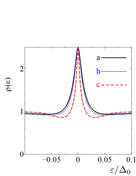
Figure 1: Normalized local density of states $\rho(\varepsilon)$ at $x=0$ by its value in the normal state is plotted as a function of $\varepsilon$. $E_{Th}=0.02\Delta_{0}$, $R_{d}/R_{b}=0.5$, and $Z=0.75$. (a)$\Delta_{p}=\Delta_{0}$ and $\Delta_{s}=0$, (b)$\Delta_{p}=0.7\Delta_{0}$ and $\Delta_{s}=0.3\Delta_{0}$, and (c)$\Delta_{p}=0.53\Delta_{0}$ and $\Delta_{s}=0.47\Delta_{0}$.

In Fig. 1, $\rho(\varepsilon)$ is plotted for $\Delta_{p}>\Delta_{s}$. The resulting $\rho(\varepsilon)$ always has a ZEP irrespective of the value of $\Delta_{s}$. It is noted that $\rho(\varepsilon=0)$ is independent of the value of $\Delta_{s}$ for $\Delta_{p}>\Delta_{s}$. We can show that $c_{1}$ and $c_{3}$ in eqs. (IV.11) and (IV.12) are proportional to $1/\varepsilon$ around $\varepsilon=0$ and satisfy $c_{1}=ic_{3}$. Then, $\zeta$ is analytically obtained as

$$\zeta=\frac{2R_{d}i}{\sigma_{N}R_{b}L}\left(x+L\right),$$ (IV.19)

independent of the magnitude of $\Delta_{s}$. The peak width of $\rho(\varepsilon)$ becomes narrower only in the regime where $\Delta_{s}$ becomes the same order to that of $\Delta_{p}$ (curve (c) in Fig. 1).

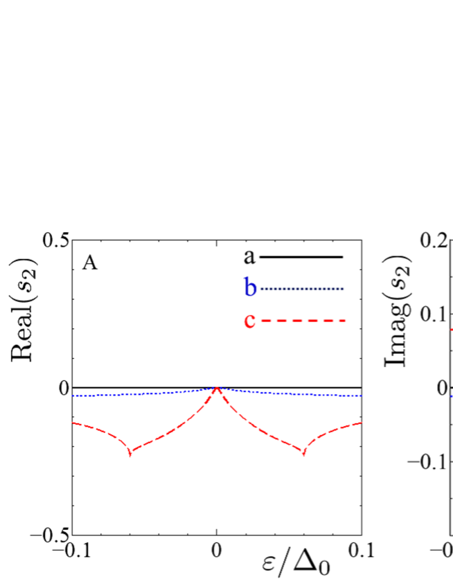
Figure 2: Real and Imaginary parts of even-frequency pair amplitude $s_{2}$ at $x=0$ is plotted as a function of $\varepsilon$ in Figs.2A and 2B, respectively. $E_{Th}=0.02\Delta_{0}$, $R_{d}/R_{b}=0.5$, and $Z=0.75$. (a)$\Delta_{p}=\Delta_{0}$ and $\Delta_{s}=0$, (b)$\Delta_{p}=0.7\Delta_{0}$ and $\Delta_{s}=0.3\Delta_{0}$, and (c)$\Delta_{p}=0.53\Delta_{0}$ and $\Delta_{s}=0.47\Delta_{0}$.

In Fig.2, the even-frequency pair amplitude $s_{2}$ is plotted for the same parameters used in Fig. 1. The real (imaginary) part of $s_{2}$ is an even (odd) function of $\varepsilon$. This $\varepsilon$ dependence is consistent with DN/$s$-wave or DN/$d$-wave superconductor junctions Tanaka et al. (2004); Tanaka and Golubov (2007). For $\Delta_{s}=0$, $s_{2}$ becomes zero [curves (a) in Figs.2A and Fig.2B] and the magnitude of $s_{2}$ is also suppressed for $\Delta_{s}=0.3\Delta_{0}$ [curves (b) in Figs.2A and Fig.2B]. Only when the magnitude of $\Delta_{s}$ becomes the same order with that of $\Delta_{p}$, $s_{2}$ is a little bit enhanced at nonzero $\varepsilon$ [curves (c) in Figs.2A and Fig.2B].

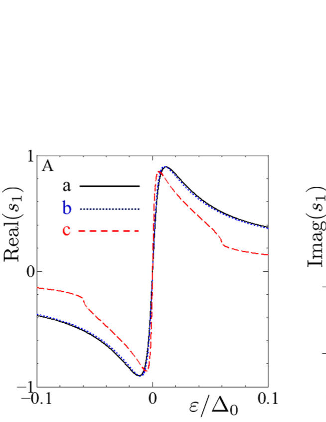
Figure 3: Real and Imaginary parts of odd-frequency pair amplitude $s_{1}$ at $x=0$ is plotted as a function of $\varepsilon$ in Figs.3A and 3B, respectively. $E_{Th}=0.02\Delta_{0}$, $R_{d}/R_{b}=0.5$, and $Z=0.75$. (a)$\Delta_{p}=\Delta_{0}$ and $\Delta_{s}=0$, (b)$\Delta_{p}=0.7\Delta_{0}$ and $\Delta_{s}=0.3\Delta_{0}$, and (c)$\Delta_{p}=0.53\Delta_{0}$ and $\Delta_{s}=0.47\Delta_{0}$.

The corresponding odd-frequency pair amplitude $s_{1}$ is shown in Fig.3. The obtained real (imaginary) part of $s_{1}$ is an odd (even) function of $\varepsilon$. These features are consistent with that in DN/p-wave superconductor junctions Tanaka and Kashiwaya (2004); Tanaka and Golubov (2007). The real part of $s_{1}$ is enhanced around $\varepsilon=0$ for all three cases (Fig. 3A). On the other hand, the magnitude of the imaginary part of $s_{1}$ has a sharp zero energy peak (ZEP) at $\varepsilon=0$. The value of $s_{1}$ at $\varepsilon=0$ is independent of $\Delta_{s}$. The peak width becomes narrower with the increase of $\Delta_{s}$ (Fig. 3B). These features are quite similar to $\rho(\varepsilon)$. Since the magnitude of $s_{1}$ exceeds that of $s_{2}$ for all cases, proximity effect in this parameter region is governed by the odd-frequency pairing even in the presence of $s$-wave pair potential.

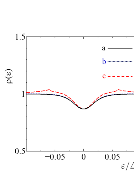
Figure 4: Normalized local density of states $\rho(\varepsilon)$ by its value in the normal state is plotted as a function of $\varepsilon$. $E_{Th}=0.02\Delta_{0}$, $R_{d}/R_{b}=0.5$, and $Z=0.75$. (a)$\Delta_{s}=\Delta_{0}$ and $\Delta_{p}=0$, (b)$\Delta_{s}=0.7\Delta_{0}$ and $\Delta_{p}=0.3\Delta_{0}$, and (c)$\Delta_{s}=0.53\Delta_{0}$ and $\Delta_{p}=0.47\Delta_{0}$.

Next, we look at the case for $\Delta_{s}>\Delta_{p}$. In Fig. 4, $\rho(\varepsilon)$ is plotted for (a)$\Delta_{s}=\Delta_{0}$ and $\Delta_{p}=0$, (b)$\Delta_{s}=0.7\Delta_{0}$ and $\Delta_{p}=0.3\Delta_{0}$, and (c)$\Delta_{s}=0.53\Delta_{0}$ and $\Delta_{p}=0.47\Delta_{0}$. $\rho(\varepsilon)$ always has a dip structure around $\varepsilon=0$. The curves (a) and (b) almost overlap each other within this energy window. The line shapes of $\rho(\varepsilon)$ is consistent with standard proximity effect in DN/$s$-wave superconductor junctions.

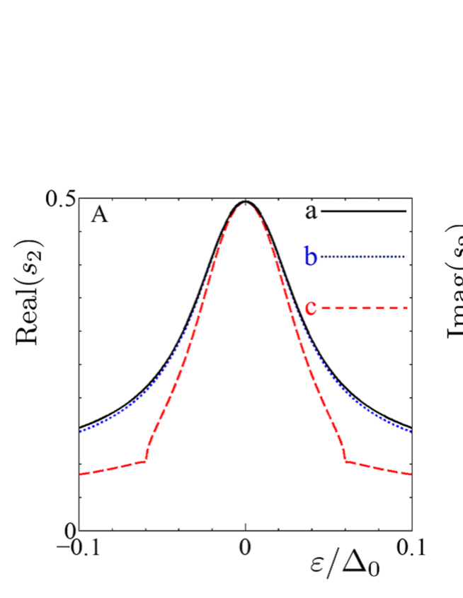
Figure 5: Real and Imaginary parts of even-frequency pair amplitude $s_{2}$ is plotted as a function of $\varepsilon$ in Figs.5A and 5B, respectively. $E_{Th}=0.02\Delta_{0}$, $R_{d}/R_{b}=0.5$, and $Z=0.75$. (a)$\Delta_{s}=\Delta_{0}$ and $\Delta_{p}=0$, (b)$\Delta_{s}=0.7\Delta_{0}$ and $\Delta_{p}=0.3\Delta_{0}$, and (c)$\Delta_{s}=0.53\Delta_{0}$ and $\Delta_{p}=0.47\Delta_{0}$.

In Fig.5, even-frequency pair amplitude $s_{2}$ is plotted for the same parameters used in the calculation of $\rho(\varepsilon)$ in Fig. 4. The real (imaginary) part of $s_{2}$ is an even(odd) function of $\varepsilon$ similar to the case of Fig. 2. As compared to the $p$-wave dominant case (Fig. 2), the magnitude of $s_{2}$ is enhanced. The real part of $s_{2}$ has a peak at $\varepsilon=0$.

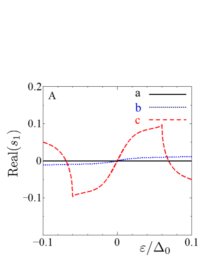
Figure 6: Real and Imaginary parts of odd-frequency pair amplitude $s_{1}$ is plotted as a function of $\varepsilon$ in Figs.6A and 6B, respectively. $E_{Th}=0.02\Delta_{0}$, $R_{d}/R_{b}=0.5$, and $Z=0.75$. (a)$\Delta_{s}=\Delta_{0}$ and $\Delta_{p}=0$, (b)$\Delta_{s}=0.7\Delta_{0}$ and $\Delta_{p}=0.3\Delta_{0}$, and (c)$\Delta_{s}=0.53\Delta_{0}$ and $\Delta_{p}=0.47\Delta_{0}$.

The corresponding odd-frequency pair amplitude $s_{1}$ is shown in Fig.6. The obtained real (imaginary) part of $s_{1}$ is an odd (even) function of $\varepsilon$ similar to the case of Fig. 3. Without $p$-wave pair potential, $s_{1}$ vanishes as shown in curve (c). As compared to $p$-wave dominant cases [curves (a)-(c) in Fig. 3], the magnitudes of $s_{1}$ are suppressed. The imaginary part of $s_{1}$ is always zero at $\varepsilon=0$. Since the magnitude of $s_{2}$ exceeds that of $s_{1}$ for all cases, proximity effect in this region is governed by even-frequency pairing even in the presence of $p$-wave pair potential.

Next, we discuss the charge conductance. From eqs. (IV.16) and (IV.3), we can show

$$\hat{R}_{1\downarrow}\left(x\right)=-\hat{\tau}_{2}\hat{R}_{1\uparrow}\left(x\right)\hat{\tau}_{2},\ \ \hat{C}_{R\downarrow}=-\hat{\tau}_{2}\hat{C}_{R\uparrow}\hat{\tau}_{2}.$$ (IV.20)

In the following, using these relations, we calculate the Keldysh component of the Green’s function. We denote $\hat{I}_{K}$ for each spin sector as $\hat{I}_{K\uparrow(\downarrow)}$. ${\rm Trace}(\hat{I}_{K\uparrow(\downarrow)}\hat{\tau}_{3})$ is expressed as

$${\rm Trace}\left[\hat{I}_{K\uparrow(\downarrow)}\hat{\tau}_{3}\right]=\frac{2\sigma_{1N}}{\mid d_{R\uparrow\left(\downarrow\right)}\mid^{2}}\left(S_{1\uparrow\left(\downarrow\right)}+S_{2\uparrow\left(\downarrow\right)}+S_{3\uparrow\left(\downarrow\right)}+S_{4\uparrow\left(\downarrow\right)}+S_{5\uparrow\left(\downarrow\right)}+S_{6\uparrow\left(\downarrow\right)}\right).$$ (IV.21)

The details of the calcuation of $S_{1\uparrow\left(\downarrow\right)}$, $S_{2\uparrow\left(\downarrow\right)}$, $S_{3\uparrow\left(\downarrow\right)}$, $S_{4\uparrow\left(\downarrow\right)}$, $S_{5\uparrow\left(\downarrow\right)}$, and $S_{6\uparrow\left(\downarrow\right)}$ in eq.(IV.21) is shown in Appendix E. Summing up the contribution from both up and down spin sectors, we obtain the following relation

$${\rm Trace}\left[\hat{I}_{k\uparrow}\hat{\tau}_{3}\right]+{\rm Trace}\left[\hat{I}_{k\downarrow}\hat{\tau}_{3}\right]$$ (IV.22)

$$= \frac{4\sigma_{1N}f_{3N}\left(x=0_{-}\right)}{\mid d_{R}\mid^{2}}$$

$$\times {\rm Trace}\left[\left(\hat{R}_{1\uparrow}+\hat{R}^{\dagger}_{1\uparrow}\right)\left(\hat{C}_{R\uparrow}+\hat{C}^{\dagger}_{R\uparrow}\right)\left(1+\sigma^{2}_{1N}\right)+2\sigma_{1N}\left(\hat{\mathbb{I}}+\hat{C}_{R\uparrow}\hat{C}^{\dagger}_{R\uparrow}\right)\right].$$

The boundary condition of the up spin sector of the Keldysh component at $x=0$ becomes

$$\left.\frac{L}{R_{d}}{\rm Trace}\left[\hat{\tau}_{3}\left(\hat{R}_{\uparrow}\left(x\right)\frac{\partial}{\partial x}\hat{K}_{\uparrow}\left(x\right)+\hat{K}_{\uparrow}\left(x\right)\frac{\partial}{\partial x}\hat{A}_{\uparrow}\left(x\right)\right)\right]\right|_{x=0_{-}}=-\frac{1}{R_{b}}{\rm Trace}\left<\left[\hat{\tau}_{3}\hat{I}_{K\uparrow}\right]\right>.$$ (IV.23)

The left side of this boundary condition becomes

$$\left.-2{\rm Imag}\left(s^{*}_{1\uparrow}s_{2\uparrow}\right)\left(\frac{\partial f_{0N}}{\partial x}\right)\right|_{x=0_{-}}\left.+2\left(1+\mid s_{1\uparrow}\mid^{2}+\mid s_{2\uparrow}\mid^{2}+\mid s_{3\uparrow}\mid^{2}\right)\left(\frac{\partial f_{3N}}{\partial x}\right)\right|_{x=0_{-}}.$$ (IV.24)

The corresponding boundary condition for down spin sector is

$$\left.\frac{L}{R_{d}}{\rm Trace}\left[\hat{\tau}_{3}\left(\hat{R}_{\downarrow}\left(x\right)\frac{\partial}{\partial x}\hat{K}_{\downarrow}\left(x\right)+\hat{K}_{\downarrow}\left(x\right)\frac{\partial}{\partial x}\hat{A}_{\downarrow}\right)\right]\right|_{x=0_{-}}=-\frac{1}{R_{b}}\left<{\rm Trace}\left[\hat{\tau}_{3}\hat{I}_{K\downarrow}\right]\right>.$$ (IV.25)

The left side of this boundary condition becomes

$$\left.-2{\rm Imag}\left(s^{*}_{1\downarrow}s_{2\downarrow}\right)\left(\frac{\partial f_{0N}}{\partial x}\right)\right|_{x=0_{-}}\left.+2\left(1+\mid s_{1\downarrow}\mid^{2}+\mid s_{2\downarrow}\mid^{2}+\mid s_{3\downarrow}\mid^{2}\right)\left(\frac{\partial f_{3N}}{\partial x}\right)\right|_{x=0_{-}}.$$ (IV.26)

Since $s_{1\uparrow}=s_{1\downarrow}=s_{1}$ and $s_{2\uparrow}=-s_{2\downarrow}=s_{2}$ are satisfied, we obtain using eqs. (IV.24) and (IV.26)

$$\left.\frac{4L}{R_{d}}\left(1+\mid s_{1}\mid^{2}+\mid s_{2}\mid^{2}+\mid s_{3}\mid^{2}\right)\left(\frac{\partial f_{3N}}{\partial x}\right)\right|_{x=0_{-}}$$ (IV.27)

$$= -\frac{1}{R_{b}}\left<{\rm Trace}\left[\hat{\tau}_{3}\left(\hat{I}_{K\uparrow}+\hat{I}_{K\downarrow}\right)\right]\right>=-\frac{8}{R_{b}}\left<I_{K}\right>,$$

with

$$I_{K}=\frac{\sigma_{1N}f_{3N}\left(x=0_{-}\right)}{2\mid d_{R}\mid^{2}}{\rm Trace}\left[\left(\hat{R}_{1\uparrow}+\hat{R}^{\dagger}_{1\uparrow}\right)\left(\hat{C}_{R\uparrow}+\hat{C}^{\dagger}_{R\uparrow}\right)\left(1+\sigma^{2}_{1N}\right)+2\sigma_{1N}\left(\hat{\mathbb{I}}+\hat{C}_{R\uparrow}\hat{C}^{\dagger}_{R\uparrow}\right)\right].$$ (IV.28)

The resulting boundary condition is given by

$$\left.\left[{\rm cosh}^{2}\zeta_{im}+\mid\sin\zeta\mid^{2}{\rm sinh}^{2}\psi_{im}\right]\left(\frac{\partial f_{3N}}{\partial x}\right)\right|_{x=0_{-}}=-\frac{R_{d}}{R_{b}L}f_{3N}\left(x=0_{-}\right)\left<I_{K}\right>$$ (IV.29)

with $\zeta_{im}={\rm Imag}\zeta$ and $\psi_{im}={\rm Imag}\psi$. Since we are considering 1d case, $\left<I_{K}\right>$ is simply given by

$$\left<I_{K}\right>=\frac{I_{K}}{\sigma_{N}}.$$

From the Keldysh part of the Usadel equation in the present case, we obtain

$$D\frac{\partial}{\partial x}{\rm Trace}\left[\hat{\tau}_{3}\left(\hat{R}_{\uparrow\left(\downarrow\right)}\frac{\partial}{\partial x}\hat{K}_{\uparrow\left(\downarrow\right)}+\hat{K}_{\uparrow\left(\downarrow\right)}\frac{\partial}{\partial x}\hat{A}_{\uparrow\left(\downarrow\right)}\right)\right]=0.$$ (IV.30)

From this equation, we obtain

$$\left.\left[{\rm cosh}^{2}\zeta_{im}+\mid\sin\zeta\mid^{2}{\rm sinh}^{2}\psi_{im}\right]\left(\frac{\partial f_{3N}\left(x=0_{-}\right)}{\partial x}\right)\right|_{x=0_{-}}=-\frac{R_{d}}{R_{b}L}f_{3N}\left(x=0_{-}\right)\left<I_{K}\right>=C_{0}.$$ (IV.31)

The electric current from both spin up and down components are given by

$$I_{e} = -\frac{L}{4eR_{d}}\int^{\infty}_{0}d\varepsilon{\rm Trace}\left[\hat{\tau}_{3}\left(\hat{R}_{1\uparrow}\frac{\partial}{\partial x}\hat{K}_{1\uparrow}+\hat{R}_{1\downarrow}\frac{\partial}{\partial x}\hat{K}_{1\downarrow}+\hat{K}_{1\uparrow}\frac{\partial}{\partial x}\hat{A}_{1\uparrow}+\hat{K}_{1\downarrow}\frac{\partial}{\partial x}\hat{A}_{1\downarrow}\right)\right]$$ (IV.32)

$$= -\frac{2L}{eR_{d}}\int^{\infty}_{0}d\varepsilon\left(\frac{\partial f_{3N}\left(x=0_{-}\right)}{\partial x}\right)F(\zeta,\psi)$$

with

$$F(\zeta,\psi)={\rm cosh}^{2}\zeta_{im}+\mid\sin\zeta\mid^{2}{\rm sinh}^{2}\psi_{im}.$$ (IV.33)

From eq. (IV.31), the following relation is satisfied

$$\left(\frac{\partial f_{3N}\left(x=0_{-}\right)}{\partial x}\right)=\frac{C_{0}}{F\left(\zeta,\psi\right)},$$ (IV.34)

we obtain

$$f_{3N}\left(0\right)\left[1+\frac{R_{d}\left<I_{K}\right>}{R_{b}L}\int^{0}_{-L}\frac{dx}{F\left(\zeta,\phi\right)}\right]=f_{3N}(x=-L)$$ (IV.35)

From eqs. (IV.31), (IV.32), (IV.34), and (IV.35), $I_{e}$ is given by

$$I_{e}=\frac{2}{e}\int^{\infty}_{0}d\varepsilon\frac{f_{3N}(x=-L)}{\frac{R_{b}}{\left<I_{K}\right>}+\frac{R_{d}}{L}\int^{0}_{-L}\frac{dx}{F\left(\zeta,\psi\right)}},$$ (IV.36)

with

$$f_{3N}\left(x=-L\right)=\frac{1}{2}\left[{\rm tanh}\left[\left(\varepsilon+eV\right)/\left(2T\right)\right]-{\rm tanh}\left[\left(\varepsilon-eV\right)/\left(2T\right)\right]\right].$$

Here, we have used units with $k_{B}=1$. At sufficiently low temperatures, total resistance of the junction is given by

$$R=\frac{1}{2}\left[\frac{R_{b}}{\left<I_{K}\right>}+\frac{R_{d}}{L}\int^{0}_{-L}\frac{dx}{F\left(\zeta,\psi\right)}\right].$$ (IV.37)

The corresponding resistance becomes

$$R_{N}=\frac{1}{2}\left(R_{d}+R_{b}\right)$$

The normalized conductance of the junction by its value in the normal state is given by

$$\sigma_{T}\left(eV\right)=\frac{R_{N}}{R}=\frac{R_{b}+R_{d}}{\frac{R_{b}}{\left<I_{K}\right>}+\frac{R_{d}}{L}\int^{0}_{-L}\frac{dx}{F\left(\zeta,\psi\right)}}.$$ (IV.38)

By denoting $\zeta(x=0)=\zeta_{N}$ and the imaginary part of $\zeta_{N}$ as $\zeta_{Ni}$, $I_{K}$ is given by

$$I_{K}=\frac{\sigma_{N}\left[2\left(2-\sigma_{N}\right)\Lambda_{c1}+\sigma_{N}\Lambda_{c2}\right]}{2\mid\Gamma_{+}\Gamma_{-}\mid\mid\left(2-\sigma_{N}\right)\left(1-\Gamma_{+}\Gamma_{-}\right)+\sigma_{N}\left[\left(1+\Gamma_{+}\Gamma_{-}\right)\cos\zeta_{N}+2i\sqrt{\Gamma_{+}\Gamma_{-}}\sin\zeta_{N}\right)\mid^{2}},$$ (IV.39)

$$\Lambda_{c1} = {\rm Real}\left[\left(\Gamma_{-}-\Gamma_{+}\right)\left(1-\Gamma^{*}_{+}\Gamma^{*}_{-}\right)\right]{\rm Imag}\left[\sqrt{\Gamma_{+}\Gamma_{-}}\left(\Gamma^{*}_{+}-\Gamma^{*}_{-}\right)\sin^{*}\zeta_{N}\right]$$ (IV.40)

$$+ {\rm Imag}\left[\left(\Gamma^{*}_{+}+\Gamma^{*}_{-}\right)\left(1-\Gamma_{+}\Gamma_{-}\right)\right]{\rm Real}\left[\sqrt{\Gamma_{+}\Gamma_{-}}\left(\Gamma^{*}_{+}+\Gamma^{*}_{-}\right)\sin^{*}\zeta_{N}\right]$$

$$+ 2{\rm Real}\left(\cos\zeta_{N}\right)\left(1-\mid\Gamma_{+}\mid^{2}\mid\Gamma_{-}\mid^{2}\right)\mid\Gamma_{+}\mid\mid\Gamma_{-}\mid,$$

$$\Lambda_{c2} = \left(1+\mid\Gamma_{+}\mid^{2}\right)\left(1+\mid\Gamma_{-}\mid^{2}\right)$$ (IV.41)

$$\times \left[4\left(1+{\rm sinh}^{2}\zeta_{Ni}\right)\mid\Gamma_{+}\mid\mid\Gamma_{-}\mid+\mid\sin\zeta_{N}\mid^{2}\left(\mid\Gamma_{+}\mid^{2}-\mid\Gamma_{-}\mid^{2}\right)\right]$$

$$+ 2{\rm Imag}\left[\sqrt{\Gamma_{+}\Gamma_{-}}\left(\Gamma^{*}_{+}+\Gamma^{*}_{-}\right)\sin^{*}\zeta_{N}\cos\zeta_{N}\right]{\rm Real}\left[\left(\Gamma_{+}+\Gamma_{-}\right)\left(1+\Gamma^{*}_{+}\Gamma^{*}_{-}\right)\right]$$

$$+ 2{\rm Real}\left[\sqrt{\Gamma_{+}\Gamma_{-}}\left(\Gamma^{*}_{+}-\Gamma^{*}_{-}\right)\sin^{*}\zeta_{N}\cos\zeta_{N}\right]{\rm Imag}\left[\left(\Gamma_{+}-\Gamma_{-}\right)\left(1+\Gamma^{*}_{+}\Gamma^{*}_{-}\right)\right]$$

$$- 2\mid\sin\zeta_{N}\mid^{2}\left(\mid\Gamma_{+}\mid^{2}-\mid\Gamma_{-}\mid^{2}\right){\rm Real}\left[\left(\Gamma_{+}-\Gamma_{-}\right)\left(\Gamma^{*}_{+}+\Gamma^{*}_{-}\right)\right],$$

using $\Gamma_{\pm}$ as defined in eq. (III.26). In Figs. 7 and 8, we plot charge conductance per a spin $\sigma_{S}(eV)$ and normalized one $\sigma_{T}(eV)$ as a function of $eV$. $\sigma_{S}(eV)$ is given by

$$\sigma_{S}(eV)=\frac{\sigma_{T}\left(eV\right)}{R_{d}+R_{b}}.$$

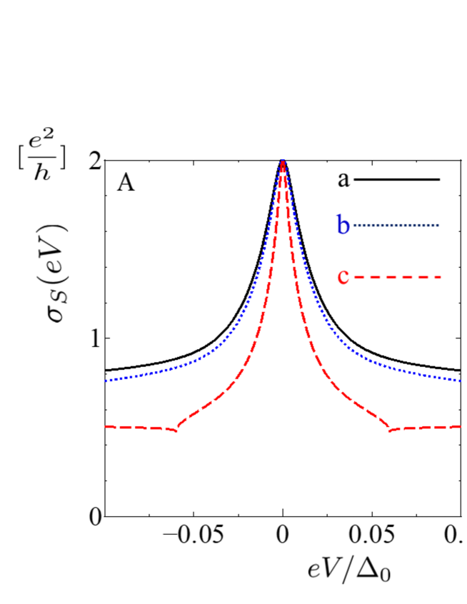
Figure 7: Charge conductance per a spin $\sigma_{S}(eV)$ and normalized one by its value in the normal state $\sigma_{T}(eV)$ is plotted as a function of $\varepsilon$ in Figs.7A and 7B, respectively. $E_{Th}=0.02\Delta_{0}$, $R_{d}/R_{b}=0.5$, and $Z=0.75$. (a)$\Delta_{p}=\Delta_{0}$ and $\Delta_{s}=0$, (b)$\Delta_{p}=0.7\Delta_{0}$ and $\Delta_{s}=0.3\Delta_{0}$, and (c)$\Delta_{p}=0.53\Delta_{0}$ and $\Delta_{s}=0.47\Delta_{0}$.

In Fig. 7, we plot $\sigma_{S}(eV)$ and $\sigma_{T}(eV)$ for $\Delta_{p}>\Delta_{s}$. In all cases, $\sigma_{S}(eV)$ has a sharp peak at $eV=0$ and $\sigma(eV=0)$ is always $2e^{2}/h$ independent of the magnitude of $\Delta_{s}$. We can explain this reason in the following. At $eV=\varepsilon=0$, $\Lambda_{c1}$ in eq. (IV.40) becomes zero since $1=\Gamma_{+}\Gamma_{-}$ is satisfied. On the other hand, $\Lambda_{c2}$ becomes

$$\Lambda_{c2}=16\left[{\rm cosh}^{2}\zeta_{Ni}+{\rm Imag}\left(\sin\zeta^{*}_{N}\cos\zeta_{N}\right)\right]=8\left[1+\exp\left(-2\zeta_{Ni}\right)\right].$$ (IV.42)

Then, we get

$$I_{K}=1+\exp\left(2\zeta_{Ni}\right).$$ (IV.43)

By using $\zeta$ calculated in eq.(IV.19) and $\psi=0$, we can show

$$\int^{0}_{-L}dx\frac{1}{{\rm\cosh}^{2}\left[\zeta_{Ni}\left(x+L\right)\right]}=\frac{\sigma_{N}R_{b}}{2}{\rm tanh}\zeta_{Ni}$$

in eq. (IV.38) with

$$\zeta_{Ni}=\frac{2R_{d}}{\sigma_{N}R_{b}L}.$$

Then, we obtain

$$\sigma_{S}(eV=0)=\frac{1}{2}R_{b}\sigma_{N}=\frac{2e^{2}}{h}.$$

This perfect resonance at zero voltage has been shown for the spin-triplet $p$-wave superconductor junction Tanaka and Kashiwaya (2004); Tanaka et al. (2005) ($\Delta_{s}=0$ in the present case) and its physical origin has been also interpreted by the index theorem Ikegaya et al. (2016). It is noted that the present perfect resonance remains even in the presence of $\Delta_{s}$. We also show the normalized value of charge conductance in its value in normal state $\sigma_{T}(eV)$ in Fig. 7B for $-1.2\Delta_{0}<eV<1.2\Delta_{0}$. $\sigma_{T}(eV)$ has a dip like structure at $\Delta_{p}\pm\Delta_{s}$.

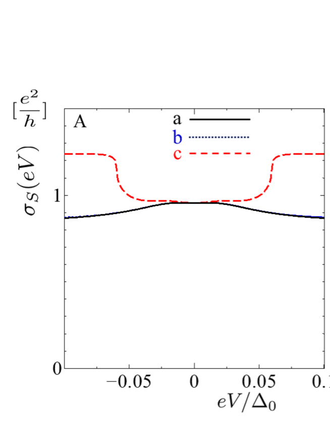
Figure 8: $\sigma_{S}(eV)$ and $\sigma_{T}(eV)$ are plotted as a function of $\varepsilon$ in Figs.8A and 8B, respectively. $E_{Th}=0.02\Delta_{0}$, $R_{d}/R_{b}=0.5$, and $Z=0.75$. (a)$\Delta_{s}=\Delta_{0}$ and $\Delta_{p}=0$, (b)$\Delta_{s}=0.7\Delta_{0}$ and $\Delta_{p}=0.3\Delta_{0}$, and (c)$\Delta_{s}=0.53\Delta_{0}$ and $\Delta_{p}=0.47\Delta_{0}$.

In Fig. 8, we plot the $\sigma_{S}(eV)$ and $\sigma_{T}(eV)$ for $\Delta_{s}>\Delta_{p}$ where even-frequency pair amplitude is dominant. Around $eV=0$, both $\sigma_{S}(eV)$ and $\sigma_{T}(eV)$ are slightly enhanced for (a)$\Delta_{p}=0$ and (b)$\Delta_{p}=0.3\Delta_{0}$. This is due to the coherent Andreev reflection in DN by conventional proximity effect by even-frequency pairing Yip (1995); Volkov et al. (1993); Tanaka et al. (2003b). For $\Delta_{p}=0.43\Delta_{0}$, this peak structure disappears. At the same time, odd-frequency pair amplitude $s_{1}$ is enhanced shown in curve (c) in Fig. 6. We also show the normalized value of charge conductance in its value in normal state $\sigma_{T}(eV)$ in Fig. 8B for $-1.2\Delta_{0}<eV<1.2\Delta_{0}$. The derivative of each curve has a sharp change at $eV=\pm\Delta_{0}$ for $\Delta_{p}=0$ [curve (c) in Fig. 8B], $eV=\pm\Delta_{0}$ and $eV=\pm 0.4\Delta_{0}$ for $\Delta_{p}=0.3\Delta_{0}$ [curve (b) in Fig. 8B], and $eV=\pm\Delta_{0}$ and $eV=\pm 0.06\Delta_{0}$ for $\Delta_{p}=0.47\Delta_{0}$ [curve (c) in Fig. 8B].

V Conclusion

In this paper, we have revisited the boundary condition of the Nambu Keldysh Green’s function in DN/unconventional superconductor junctions. We have derived a more compact expression of the boundary condition of the Nambu-Keldysh Green’s function and shown that it is consistent with the formal boundary condition of Green’s function derived by Zaitsev Zaitsev (1984). We have shown both retarded part and Keldysh part of the boundary condition available for general situation including mixed parity cases. We have demonstrated a clearer and shorter way to derive the expression for the charge conductance of the junction both for spin-singlet or spin-triplet superconductor cases studied before Tanaka et al. (2004, 2005). By applying this formula to a one-dimensional $s+p$-wave superconductor model, we have calculated LDOS, pair amplitude and charge conductance. When the $s$-wave component of the pair potential is dominant, the dominant pairing in DN is even-frequency spin-singlet $s$-wave one and the local density of states (LDOS) of quasiparticle have a minimum at zero energy. On the other hand, when spin-triplet $p$-wave component is dominant, the dominant pairing in DN is odd-frequency spin-triplet $s$-wave and LDOS has a zero energy peak. We have shown the robustness of the quantization of the conductance when the magnitude of the $p$-wave component of the pair potential is larger than that of $s$-wave one. These results show that the anomalous proximity effect owing to the odd-frequency pairing is robust with respect to the inclusion of $s$-wave component of the pair potential when the $p$-wave one is dominant. In this paper, in order to understand the essence of the crossover of the proximity effect from anomalous one due to the odd-frequency pairing to conventional one by the even-frequency pairing, we have used a one-dimensional model. Extension to two-dimensional model of $s+p_{x}$-wave superconductor is an important forthcoming work. As a $p$-wave pair potential, it is a challenging issue to choose chiral $p$-wave and helical $p$-wave pairing. Up to now, charge transport has been calculated in $s$ + chiral $p$-wave and $s$ + helical $p$-wave superconductor junction in the ballistic limit Burset et al. (2014); Tanaka et al. (2009). It is timely to study the proximity effect in these junctions. Extension of the present work to diffusive ferromagnet (DF) / $s+p$-wave junction is also an interesting topic Yokoyama et al. (2007) from the view point of superconducting spintronics Eschrig (2015); Linder and Robinson (2015).

VI Appendix A

Here, we explain the derivation of $\check{I}_{n}$ in Tanaka et al. (2003a) step by step Tanaka (2021). We choose the basis in order to diagonalize $\bar{Q}$. Then, $\bar{G}_{2}$ can be written as

$$\bar{G}_{2}=\begin{pmatrix}\check{H}_{+}&\check{0}\\ \check{0}&\check{H}_{+}\end{pmatrix}+\begin{pmatrix}\check{H}_{-}&\check{0}\\ \check{0}&\check{H}_{-}\end{pmatrix}\bar{\Sigma}^{z}.$$

Using the basis which diagonalizes $\bar{Q}$, $\bar{g}_{2}$ is obtained as shown in (II.12)Tanaka et al. (2003a, 2004) with

$$\bar{\Sigma}_{z}=\begin{pmatrix}\check{0}&\check{\mathbb{I}}\\ \check{\mathbb{I}}&\check{0}\end{pmatrix}.$$

The matrix current $\check{I}_{n}$

$$\check{I}_{n}\equiv{\rm Tr}\left[\bar{\Sigma}^{z}\bar{g}_{2}\right]$$

is obtained as

$$\check{I}_{n}= \left[\check{H}_{-}-\left(q_{n}^{-1}\check{H}_{+}+\check{G}_{1}\right)\check{H}_{-}^{-1}\left(q_{n}\check{H}_{+}+\check{G}_{1}\right)\right]^{-1}\left(2\check{\mathbb{I}}-\check{H}_{-}\right)$$

$$+ \left[\check{H}_{-}-\left(q_{n}\check{H}_{+}+\check{G}_{1}\right)\check{H}_{-}^{-1}\left(q_{n}^{-1}\check{H}_{+}+\check{G}_{1}\right)\right]^{-1}\left(2\check{\mathbb{I}}-\check{H}_{-}\right)$$

$$+ \left[\left(q_{n}\check{H}_{+}+\check{G}_{1}\right)-\check{H}_{-}\left(q_{n}^{-1}\check{H}_{+}+\check{G}_{1}\right)^{-1}\check{H}_{-}\right]^{-1}\left(\check{G}_{1}-q_{n}\check{H}_{+}\right)$$

$$+ \left[\left(q_{n}^{-1}\check{H}_{+}+\check{G}_{1}\right)-\check{H}_{-}\left(q_{n}\check{H}_{+}+\check{G}_{1}\right)^{-1}\check{H}_{-}\right]^{-1}\left(\check{G}_{1}-q_{n}^{-1}\check{H}_{+}\right)$$

$$= \left[\check{H}_{-}-\left(q_{n}\check{H}_{+}+\check{G}_{1}\right)\check{H}_{-}^{-1}\left(q_{n}^{-1}\check{H}_{+}+\check{G}_{1}\right)\right]^{-1}$$

$$\times \left[\left(2\check{\mathbb{I}}-\check{H}_{-}\right)-\left(q_{n}\check{H}_{+}+\check{G}_{1}\right)\check{H}_{-}^{-1}\left(\check{G}_{1}-q_{n}^{-1}\check{H}_{+}\right)\right]$$

$$+ \left[\check{H}_{-}-\left(q_{n}^{-1}\check{H}_{+}+\check{G}_{1}\right)\check{H}_{-}^{-1}\left(q_{n}\check{H}_{+}+\check{G}_{1}\right)\right]^{-1}$$

$$\times \left[\left(2\check{\mathbb{I}}-\check{H}_{-}\right)-\left(q_{n}^{-1}\check{H}_{+}+\check{G}_{1}\right)\check{H}_{-}^{-1}\left(\check{G}_{1}-q_{n}\check{H}_{+}\right)\right].$$ (VI.1)

By using the following relations between $\check{H}_{-}$ and $\check{H}_{+}$,

$$\check{H}_{-}-\check{H}_{+}\check{H}^{-1}_{-}\check{H}_{+}=\check{H}^{-1}_{-},\ \ \check{H}_{-}\check{H}_{+}=-\check{H}_{+}\check{H}_{-},$$

$\check{I}_{n}$ is transformed as

$$\check{I}_{n} =\left[\check{H}_{-}^{-1}-\check{G}_{1}\check{H}_{-}^{-1}\check{G}_{1}-\frac{1}{q_{n}}\check{G}_{1}\check{H}_{-}^{-1}\check{H}_{+}-q_{n}\check{H}_{+}\check{H}_{-}^{-1}\check{G}_{1}\right]^{-1}$$

$$\times\left[2\check{\mathbb{I}}-\check{H}_{-}^{-1}-\check{G}_{1}\check{H}_{-}^{-1}\check{G}_{1}+\frac{1}{q_{n}}\check{G}_{1}\check{H}_{-}^{-1}\check{H}_{+}+q_{n}\check{H}_{-}^{-1}\check{H}_{+}\check{G}_{1}\right]$$

$$+\left[\check{H}_{-}^{-1}-\check{G}_{1}\check{H}_{-}^{-1}\check{G}_{1}-q_{n}\check{G}_{1}\check{H}_{-}^{-1}\check{H}_{+}-\frac{1}{q_{n}}\check{H}_{+}\check{H}_{-}^{-1}\check{G}_{1}\right]^{-1}$$

$$\times\left[2\check{\mathbb{I}}-\check{H}_{-}^{-1}-\check{G}_{1}\check{H}_{-}^{-1}\check{G}_{1}+q_{n}\check{G}_{1}\check{H}_{-}^{-1}\check{H}_{+}+\frac{1}{q_{n}}\check{H}_{-}^{-1}\check{H}_{+}\check{G}_{1}\right]$$

$$=\frac{1}{2}\left[\check{H}_{-}^{-1}-\check{G}_{1}\check{H}_{-}^{-1}\check{G}_{1}-\frac{1}{q_{n}}\check{G}_{1}\check{H}_{-}^{-1}\check{H}_{+}-q_{n}\check{H}_{+}\check{H}_{-}^{-1}\check{G}_{1}\right]^{-1}$$

$$\times\biggl{[}-\left(\check{H}_{-}^{-1}-\check{G}_{1}\check{H}_{-}^{-1}\check{G}_{1}-\frac{1}{q_{n}}\check{G}_{1}\check{H}_{-}^{-1}\check{H}_{+}-q_{n}\check{H}_{+}\check{H}_{-}^{-1}\check{G}_{1}\right)$$

$$\phantom{\times}+2\left(\check{\mathbb{I}}-\check{G}_{1}\check{H}_{-}^{-1}\check{G}_{1}+q_{n}\check{H}_{-}^{-1}\check{H}_{+}\check{G}_{1}\right)\biggr{]}$$

$$+\frac{1}{2}\left[\check{H}_{-}^{-1}-\check{G}_{1}\check{H}_{-}^{-1}\check{G}_{1}-\frac{1}{q_{n}}\check{G}_{1}\check{H}_{-}^{-1}\check{H}_{+}-q_{n}\check{H}_{+}\check{H}_{-}^{-1}\check{G}_{1}\right]^{-1}$$

$$\times\biggl{[}\left(\check{H}_{-}^{-1}-\check{G}_{1}\check{H}_{-}^{-1}\check{G}_{1}-\frac{1}{q_{n}}\check{G}_{1}\check{H}_{-}^{-1}\check{H}_{+}-q_{n}\check{H}_{+}\check{H}_{-}^{-1}\check{G}_{1}\right)$$

$$\phantom{\times}+2\left(\check{\mathbb{I}}-\check{H}_{-}^{-1}+\frac{1}{q_{n}}\check{G}_{1}\check{H}_{-}^{-1}\check{H}_{+}\right)\biggr{]}$$

$$+\frac{1}{2}\left[\check{H}_{-}^{-1}-\check{G}_{1}\check{H}_{-}^{-1}\check{G}_{1}-q_{n}\check{G}_{1}\check{H}_{-}^{-1}\check{H}_{+}-\frac{1}{q_{n}}\check{H}_{+}\check{H}_{-}^{-1}\check{G}_{1}\right]^{-1}$$

$$\times\biggl{[}-\left(\check{H}_{-}^{-1}-\check{G}_{1}\check{H}_{-}^{-1}\check{G}_{1}-q_{n}\check{G}_{1}\check{H}_{-}^{-1}\check{H}_{+}-\frac{1}{q_{n}}\check{H}_{+}\check{H}_{-}^{-1}\check{G}_{1}\right)$$

$$\phantom{\times}+2\left(\check{\mathbb{I}}-\check{G}_{1}\check{H}_{-}^{-1}\check{G}_{1}+\frac{1}{q_{n}}\check{H}_{-}^{-1}\check{H}_{+}\check{G}_{1}\right)\biggr{]}$$

$$+\frac{1}{2}\left[\check{H}_{-}^{-1}-\check{G}_{1}\check{H}_{-}^{-1}\check{G}_{1}-q_{n}\check{G}_{1}\check{H}_{-}^{-1}\check{H}_{+}-\frac{1}{q_{n}}\check{H}_{+}\check{H}_{-}^{-1}\check{G}_{1}\right]^{-1}$$

$$\times\biggl{[}\left(\check{H}_{-}^{-1}-\check{G}_{1}\check{H}_{-}^{-1}\check{G}_{1}-q_{n}\check{G}_{1}\check{H}_{-}^{-1}\check{H}_{+}-\frac{1}{q_{n}}\check{H}_{+}\check{H}_{-}^{-1}\check{G}_{1}\right)$$

$$\phantom{\times}+2\left(\check{\mathbb{I}}-\check{H}_{-}^{-1}+q_{n}\check{G}_{1}\check{H}_{-}^{-1}\check{H}_{+}\right)\biggr{]}.$$ (VI.2)

Applying the normalization condition of $\check{G}_{1}$ given by $\check{G}_{1}^{2}=\check{\mathbb{I}}$, we obtain

$$\check{I}_{n}=$$

$$\left[\check{H}_{-}^{-1}-\check{G}_{1}\check{H}_{-}^{-1}\check{G}_{1}-\frac{1}{q_{n}}\check{G}_{1}\check{H}_{-}^{-1}\check{H}_{+}+q_{n}\check{H}_{-}^{-1}\check{H}_{+}\check{G}_{1}\right]^{-1}\!\left[\check{\mathbb{I}}-\check{G}_{1}\check{H}_{-}^{-1}\check{G}_{1}+q_{n}\check{H}_{-}^{-1}\check{H}_{+}\check{G}_{1}\right]$$

$$+\!\left[\check{H}_{-}^{-1}-\check{G}_{1}\check{H}_{-}^{-1}\check{G}_{1}-\frac{1}{q_{n}}\check{G}_{1}\check{H}_{-}^{-1}\check{H}_{+}+q_{n}\check{H}_{-}^{-1}\check{H}_{+}\check{G}_{1}\right]^{-1}\!\!\left[\check{\mathbb{I}}-\check{H}_{-}^{-1}+\frac{1}{q_{n}}\check{G}_{1}\check{H}_{-}^{-1}\check{H}_{+}\right]$$

$$+\!\left[\check{H}_{-}^{-1}-\check{G}_{1}\check{H}_{-}^{-1}\check{G}_{1}-q_{n}\check{G}_{1}\check{H}_{-}^{-1}\check{H}_{+}+\frac{1}{q_{n}}\check{H}_{-}^{-1}\check{H}_{+}\check{G}_{1}\right]^{-1}\!\!\left[\check{\mathbb{I}}-\check{G}_{1}\check{H}_{-}^{-1}\check{G}_{1}+\frac{1}{q_{n}}\check{H}_{-}^{-1}\check{H}_{+}\check{G}_{1}\!\right]$$

$$+\!\left[\check{H}_{-}^{-1}-\check{G}_{1}\check{H}_{-}^{-1}\check{G}_{1}-q_{n}\check{G}_{1}\check{H}_{-}^{-1}\check{H}_{+}+\frac{1}{q_{n}}\check{H}_{-}^{-1}\check{H}_{+}\check{G}_{1}\right]^{-1}\!\left[\check{\mathbb{I}}-\check{H}_{-}^{-1}+q_{n}\check{G}_{1}\check{H}_{-}^{-1}\check{H}_{+}\right]$$

$$=\left\{q_{n}\!\left[\check{G}_{1},\check{H}_{-}^{-1}\right]-\check{H}_{-}^{-1}\check{H}_{+}+q_{n}^{2}\check{G}_{1}\check{H}_{-}^{-1}\check{H}_{+}\check{G}_{1}\right\}^{-1}\!\left[q_{n}\!\left(\check{G}_{1}-\check{H}_{-}^{-1}\check{G}_{1}\right)+q_{n}^{2}\check{G}_{1}\check{H}_{-}^{-1}\check{H}_{+}\check{G}_{1}\right]$$

$$+\left\{q_{n}\!\left[\check{G}_{1},\check{H}_{-}^{-1}\right]-\check{H}_{-}^{-1}\check{H}_{+}+q_{n}^{2}\check{G}_{1}\check{H}_{-}^{-1}\check{H}_{+}\check{G}_{1}\right\}^{-1}\!\left[q_{n}\!\left(\check{G}_{1}-\check{G}_{1}\check{H}_{-}^{-1}\right)+\check{H}_{-}^{-1}\check{H}_{+}\right]$$

$$+\!\left\{\frac{1}{q_{n}}\left[\check{G}_{1},\check{H}_{-}^{-1}\right]-\check{H}_{-}^{-1}\check{H}_{+}+\frac{1}{q_{n}^{2}}\check{G}_{1}\check{H}_{-}^{-1}\check{H}_{+}\check{G}_{1}\right\}^{-1}$$

$$\phantom{+}\times\!\left[\frac{1}{q_{n}}\left(\check{G}_{1}-\check{H}_{-}^{-1}\check{G}_{1}\right)+\frac{1}{q_{n}^{2}}\check{G}_{1}\check{H}_{-}^{-1}\check{H}_{+}\check{G}_{1}\right]$$

$$+\!\left\{\frac{1}{q_{n}}\left[\check{G}_{1},\check{H}_{-}^{-1}\right]-\check{H}_{-}^{-1}\check{H}_{+}+\frac{1}{q_{n}^{2}}\check{G}_{1}\check{H}_{-}^{-1}\check{H}_{+}\check{G}_{1}\right\}^{-1}\!\left[\frac{1}{q_{n}}\left(\check{G}_{1}-\check{G}_{1}\check{H}_{-}^{-1}\right)+\check{H}^{-1}_{-}\check{H}_{+}\right].$$ (VI.3)

Since $q_{n}$ is expressed by $\sigma_{N}$,

$$q_{n}=\sigma_{N}/(1-\sqrt{1-\sigma_{N}})^{2},$$

the relations

$$\frac{1}{\left(1+q_{n}\right)^{2}}=\frac{1}{4}\left(1-\sqrt{1-\sigma_{N}}\right)^{2},\quad\frac{q_{n}}{\left(1+q_{n}\right)^{2}}=\frac{\sigma_{N}}{4},\quad\frac{q_{n}^{2}}{\left(1+q_{n}\right)^{2}}=\frac{1}{4}\left(1+\sqrt{1-\sigma_{N}}\right)^{2}$$

are satisfied. By using these relations, $\check{I}_{n}$ is given by

$$\check{I}_{n}=\left\{\sigma_{N}\left[\check{G}_{1},\check{H}_{-}^{-1}\right]-(1-\sqrt{1-\sigma_{N}})^{2}\check{H}_{-}^{-1}\check{H}_{+}+(1+\sqrt{1-\sigma_{N}})^{2}\check{G}_{1}\check{H}_{-}^{-1}\check{H}_{+}\check{G}_{1}\right\}^{-1}$$

$$\times\!\left[\sigma_{N}\!\left(2\check{G}_{1}-\left[\check{H}^{-1}_{-},\check{G}_{1}\right]_{+}\right)\!+\left(1+\sqrt{1-\sigma_{N}}\right)^{2}\check{G}_{1}\check{H}_{-}^{-1}\check{H}_{+}\check{G}_{1}+\left(1-\sqrt{1-\sigma_{N}}\right)^{2}\!\check{H}_{-}^{-1}\check{H}_{+}\right]$$

$$+\left\{\sigma_{N}\left[\check{G}_{1},\check{H}_{-}^{-1}\right]-(1+\sqrt{1-\sigma_{N}})^{2}\check{H}_{-}^{-1}\check{H}_{+}+(1-\sqrt{1-\sigma_{N}})^{2}\check{G}_{1}\check{H}_{-}^{-1}\check{H}_{+}\check{G}_{1}\right\}^{-1}$$

$$\times\!\left[\sigma_{N}\!\left(2\check{G}_{1}-\left[\check{H}_{-}^{-1},\check{G}_{1}\right]_{+}\right)\!+\left(1-\sqrt{1-\sigma_{N}}\right)^{2}\check{G}_{1}\check{H}_{-}^{-1}\check{H}_{+}\check{G}_{1}+\left(1+\sqrt{1-\sigma_{N}}\right)^{2}\!\check{H}_{-}^{-1}\check{H}_{+}\right]$$

Here, by using $\sigma_{1N}=\sigma_{N}/(1+\sqrt{1-\sigma_{N}})^{2}$,

$$\sigma_{1N}^{2}=\left(\frac{1-\sqrt{1-\sigma_{N}}}{1+\sqrt{1-\sigma_{N}}}\right)^{2}$$

is satisfied and $\check{I}_{n}$ is expressed using $\sigma_{1N}$ as follows.

$$\check{I}_{n} =\left\{\sigma_{1N}\left[\check{G}_{1},\check{H}_{-}^{-1}\right]-\sigma_{1N}^{2}\check{H}_{-}^{-1}\check{H}_{+}+\check{G}_{1}\check{H}_{-}^{-1}\check{H}_{+}\check{G}_{1}\right\}^{-1}$$

$$\phantom{=}\times\left\{\sigma_{1N}\left(2\check{G}_{1}-\left[\check{H}_{-}^{-1},\check{G}_{1}\right]_{+}\right)+\sigma_{1N}^{2}\check{H}_{-}^{-1}\check{H}_{+}+\check{G}_{1}\check{H}_{-}^{-1}\check{H}_{+}\check{G}_{1}\right\}$$

$$+\left\{\sigma_{1N}\left[\check{G}_{1},\check{H}_{-}^{-1}\right]-\check{H}_{-}^{-1}\check{H}_{+}+\sigma_{1N}^{2}\check{G}_{1}\check{H}_{-}^{-1}\check{H}_{+}\check{G}_{1}\right\}^{-1}$$

$$\phantom{=}\times\left\{\sigma_{1N}\left(2\check{G}_{1}-\left[\check{H}_{-}^{-1},\check{G}_{1}\right]_{+}\right)+\check{H}_{-}^{-1}\check{H}_{+}+\sigma_{1N}^{2}\check{G}_{1}\check{H}_{-}^{-1}\check{H}_{+}\check{G}_{1}\right\}$$

$$=\left\{\sigma_{1N}\left[\check{G}_{1},\check{H}_{-}^{-1}\right]-\sigma_{1N}^{2}\check{H}_{-}^{-1}\check{H}_{+}+\check{G}_{1}\check{H}_{-}^{-1}\check{H}_{+}\check{G}_{1}\right\}^{-1}$$

$$\phantom{=}\times\{\left[\sigma_{1N}\left[\check{G}_{1},\check{H}_{-}^{-1}\right]-\sigma_{1N}^{2}\check{H}_{-}^{-1}\check{H}_{+}+\check{G}_{1}\check{H}_{-}^{-1}\check{H}_{+}\check{G}_{1}\right]$$

$$\phantom{=}+2\sigma_{1N}\left(\check{G}_{1}-\check{G}_{1}\check{H}_{-}^{-1}\right)+2\sigma_{1N}^{2}\check{H}^{-1}_{-}\check{H}_{+}\}$$

$$+\left\{\sigma_{1N}\left[\check{G}_{1},\check{H}_{-}^{-1}\right]-\check{H}_{-}^{-1}\check{H}_{+}+\sigma_{1N}^{2}\check{G}_{1}\check{H}_{-}^{-1}\check{H}_{+}\check{G}_{1}\right\}^{-1}$$

$$\phantom{=}\times\{-\left[\sigma_{1N}\left[\check{G}_{1},\check{H}_{-}^{-1}\right]-\check{H}_{-}^{-1}\check{H}_{+}+\sigma_{1N}^{2}\check{G}_{1}\check{H}_{-}^{-1}\check{H}_{+}\check{G}_{1}\right]$$

$$\phantom{=}+2\sigma_{1N}\left(\check{G}_{1}-\check{H}_{-}^{-1}\check{G}_{1}\right)+2\sigma_{1N}^{2}\check{G}_{1}\check{H}_{-}^{-1}\check{H}_{+}\check{G}_{1}\}$$

$$=2\left\{\sigma_{1N}\left[\check{G}_{1},\check{H}_{-}^{-1}\right]-\sigma_{1N}^{2}\check{H}_{-}^{-1}\check{H}_{+}+\check{G}_{1}\check{H}_{-}^{-1}\check{H}_{+}\check{G}_{1}\right\}^{-1}$$

$$\phantom{=}\times\left\{\sigma_{1N}\left(\check{G}_{1}-\check{G}_{1}\check{H}_{-}^{-1}\right)+\sigma_{1N}^{2}\check{H}^{-1}_{-}\check{H}_{+}\right\}$$

$$+2\left\{\sigma_{1N}\left[\check{G}_{1},\check{H}_{-}^{-1}\right]-\check{H}_{-}^{-1}\check{H}_{+}+\sigma_{1N}^{2}\check{G}_{1}\check{H}_{-}^{-1}\check{H}_{+}\check{G}_{1}\right\}^{-1}$$

$$\phantom{=}\times\left\{\sigma_{1N}\left(\check{G}_{1}-\check{H}_{-}^{-1}\check{G}_{1}\right)+\sigma_{1N}^{2}\check{G}_{1}\check{H}_{-}^{-1}\check{H}_{+}\check{G}_{1}\right\}$$ (VI.4)

If we define $\check{A}_{c}$ and $\check{A}_{a}$ as

$$\check{A}_{c}\equiv -\left\{\sigma_{1N}\left[\check{G}_{1},\check{H}_{-}^{-1}\right]-\sigma_{1N}^{2}\check{H}_{-}^{-1}\check{H}_{+}+\check{G}_{1}\check{H}_{-}^{-1}\check{H}_{+}\check{G}_{1}\right\}^{-1}$$

$$\times\left\{\sigma_{1N}\left(\check{G}_{1}-\check{G}_{1}\check{H}_{-}^{-1}\right)+\sigma_{1N}^{2}\check{H}^{-1}_{-}\check{H}_{+}\right\}$$

$$\check{A}_{a}\equiv -\left\{\sigma_{1N}\left[\check{G}_{1},\check{H}_{-}^{-1}\right]-\check{H}_{-}^{-1}\check{H}_{+}+\sigma_{1N}^{2}\check{G}_{1}\check{H}_{-}^{-1}\check{H}_{+}\check{G}_{1}\right\}^{-1}$$

$$\times\left\{\sigma_{1N}\left(\check{G}_{1}-\check{H}_{-}^{-1}\check{G}_{1}\right)+\sigma_{1N}^{2}\check{G}_{1}\check{H}_{-}^{-1}\check{H}_{+}\check{G}_{1}\right\}$$

$\check{A}_{c}=-\check{G}_{1}\check{A}_{a}\check{G}_{1}$ is satisfied. Here, defining

$$\check{B}\equiv\check{A}_{a}\check{G}_{1}$$

$\check{I}_{n}$ is expressed by

$$\check{I}_{n}=2\left[\check{G}_{1},\check{B}\right]$$

with

$$\check{B}=\left(\check{H}_{-}^{-1}\check{H}_{+}-\sigma_{1N}\left[\check{G}_{1},\check{H}_{-}^{-1}\right]-\sigma_{1N}^{2}\check{G}_{1}\check{H}_{-}^{-1}\check{H}_{+}\check{G}_{1}\right)^{-1}\left\{\sigma_{1N}\left(\check{\mathbb{I}}-\check{H}_{-}^{-1}\right)+\sigma_{1N}^{2}\check{G}_{1}\check{H}_{-}^{-1}\check{H}_{+}\right\}.$$ (VI.5)

VII Appendix B

In this section, we show that our obtained boundary condition is consistent with Zaitsev’s one Zaitsev (1984) although we are considering unconventional superconductor junctions. Zaitsev disussed the boundary condition of quasiclassical Green’s function as shown in Fig. 9 assuming a spin-singlet $s$-wave pair potential. He defined $\check{g}_{1}^{s}$, $\check{g}_{1}^{a}$, $\check{g}_{2}^{s}$, $\check{g}_{2}^{a}$ as

$$\check{g}_{1}^{s}=\frac{1}{2}\left(\check{g}_{1}^{+}+\check{g}_{1}^{-}\right),\ \ \check{g}_{1}^{a}=\frac{1}{2}\left(\check{g}_{1}^{+}-\check{g}_{1}^{-}\right),$$ (VII.1)

and

$$\check{g}_{2}^{s}=\frac{1}{2}\left(\check{g}_{2}^{+}+\check{g}_{2}^{-}\right),\ \check{g}_{2}^{a}=\frac{1}{2}\left(\check{g}_{2}^{+}-\check{g}_{2}^{-}\right),$$ (VII.2)

both left and right sides.

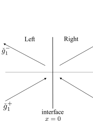
Figure 9: Schematic picture showing trajectory of quasiclassical Green’s function, $\check{g}_{1}^{+}$, $\check{g}_{1}^{-}$, $\check{g}_{2}^{+}$, and $\check{g}_{2}^{-}$. Left and right corresponds to normal metal or superconductor.

By using these functions, $\check{g}_{s}^{+}$ and $\check{g}_{s}^{-}$ are defined at the interface as

$$\check{g}_{s}^{+}\equiv\frac{1}{2}\left(\check{g}_{1}^{s}+\check{g}_{2}^{s}\right),\\ \check{g}_{s}^{-}\equiv\frac{1}{2}\left(\check{g}_{1}^{s}-\check{g}_{2}^{s}\right).$$ (VII.3)

The Zaitsev’s boundary condition is given by

$$\check{g}_{a}=\check{g}_{1}^{a}=\check{g}_{2}^{a},\ \$$ (VII.4)

$$\check{g}_{a}\left[\left(1-\sigma_{N}\right)\left(\check{g}_{s}^{+}\right)^{2}+\left(\check{g}_{s}^{-}\right)^{2}\right]=\sigma_{N}\check{g}_{s}^{-}\check{g}_{s}^{+}$$ (VII.5)

by using the transmissivity at the interface $\sigma_{N}$. In the following,it is shown that our obtained boundary condition of Nambu-Keldysh Green’s function is consistent with Zaitsev’s one.

For this purpose, we must start from so called interface matrix $\bar{g}_{2}$ defined in eq.(II.12). It is written as

$$\bar{g}_{2}=\left(\begin{array}[]{cc}q_{n}\check{H}_{+}+\check{G}_{1}&q_{n}\check{H}_{-}\\ q_{n}^{-1}\check{H}_{-}&q_{n}^{-1}\check{H}_{+}+\check{G}_{1}\end{array}\right)^{-1}\left(\begin{array}[]{cc}q_{n}\left(2\check{\mathbb{I}}-\check{H}_{-}\right)&\ \check{G}_{1}-q_{n}\check{H}_{+}\\ \check{G}_{1}-q_{n}^{-1}\check{H}_{+}&\ q_{n}^{-1}\left(2\check{\mathbb{I}}-\check{H}_{-}\right)\end{array}\right)$$ (VII.6)

The matrix current is defined by

$$\check{I}_{n}={\rm Trace}\left[\bar{\Sigma}^{z}\bar{g}_{2}\right].$$

As shown in eq. (II.25), $\check{I}_{n}$ is expressed by

$$\check{I}_{n}=2\sigma_{N}\left[\left(4-2\sigma_{N}\right)\check{\mathbb{I}}+\sigma_{N}[\check{C},\check{G}_{1}]_{+}\right]^{-1}\left[\check{C},\check{G}_{1}\right]$$ (VII.7)

Next, we calculate ${\rm Trace}[\bar{g}_{2}]$. After a straightforward transformation,

$${\rm Trace}\left[\bar{g}_{2}\right]\noindent$$ (VII.8)

$$= 2\left\{\sigma_{1N}\left[\check{G}_{1},\check{H}_{-}^{-1}\right]-\check{H}_{-}^{-1}\check{H}_{+}-\sigma_{1N}^{2}\check{G}_{1}\check{H}_{+}\check{H}_{-}^{-1}\check{G}_{1}\right\}^{-1}\noindent$$ (VII.9)

$$\times \left[\check{\mathbb{I}}-\sigma_{1N}\check{G}_{1}\check{H}_{+}\check{H}_{-}^{-1}-\check{H}_{-}^{-1}\right]\noindent$$ (VII.10)

$$+ 2\sigma_{1N}\left\{\sigma_{1N}\left[\check{G}_{1},\check{H}_{-}^{-1}\right]-\sigma_{1N}^{2}\check{H}_{-}^{-1}\check{H}_{+}-\check{G}_{1}\check{H}_{+}\check{H}_{-}^{-1}\check{G}_{1}\right\}^{-1}\noindent$$ (VII.11)

$$\times \left[\sigma_{1N}\check{\mathbb{I}}-\check{G}_{1}\check{H}_{+}\check{H}_{-}^{-1}-\sigma_{1N}\check{H}_{-}^{-1}\right]$$ (VII.12)

Following the same procedure used in the calculation of ${\rm Trace}[\bar{g}_{2}\Sigma^{z}]$, we obtain ${\rm Trace}[\bar{g}_{2}]$

$${\rm Trace}\left[\bar{g}_{2}\right]\noindent$$ (VII.13)

$$= 2\left\{\left(1+\sigma^{2}_{1N}\right)\check{\mathbb{I}}+\sigma_{1N}\left[\check{C},\check{G}_{1}\right]_{+}\right\}^{-1}\left[\check{C}\left(1+\sigma_{1N}^{2}\right)+2\sigma_{1N}\check{G}_{1}\right]\noindent$$ (VII.14)

$$= 4\left\{2\left(2-\sigma_{N}\right)\check{\mathbb{I}}+\sigma_{N}\left[\check{C},\check{G}_{1}\right]_{+}\right\}^{-1}\left[\left(2-\sigma_{N}\right)\check{C}+\sigma_{N}\check{G}_{1}\right]$$ (VII.15)

Then, let us look at $\bar{g}_{1}$. It can be calculated similar to $\bar{g}_{1}$ and is given by

$$\bar{g}_{1}=\begin{pmatrix}\frac{1}{q_{n}}\left(2\check{\mathbb{I}}+\check{H}_{-}\right)&\check{H}_{+}+q_{n}\check{G}_{1}\\ \check{H}_{+}+\frac{1}{q_{n}}\check{G}_{1}&q_{n}\left(2\check{\mathbb{I}}+\check{H}_{-}\right)\end{pmatrix}\begin{pmatrix}\check{H}_{+}+\frac{1}{q_{n}}\check{G}_{1}&q_{n}\}\check{G}_{1}\\ \frac{1}{q_{n}}\check{G}_{1}&\check{H}_{+}+q_{n}\check{G}_{1}\end{pmatrix}$$ (VII.16)

${\rm Trace}[\bar{g}_{1}]$ and ${\rm Trace}[\bar{g}_{1}\Sigma^{z}]$ can be calculated in the similar way.

$${\rm Trace}\left[\bar{g}_{1}\Sigma^{z}\right]$$ (VII.17)

$$= 2\sigma_{N}\left[\left(4-2\sigma_{N}\right)\check{\mathbb{I}}+\sigma_{N}[\check{C},\check{G}_{1}]_{+}\right]^{-1}\left[\check{C},\check{G}_{1}\right]$$

$${\rm Trace}\left[\bar{g}_{1}\right]$$ (VII.18)

$$= 4\left\{2\left(2-\sigma_{N}\right)\check{\mathbb{I}}+\sigma_{N}\left[\check{C},\check{G}_{1}\right]_{+}\right\}^{-1}\left[\left(2-\sigma_{N}\right)\check{G}_{1}+\sigma_{N}\check{C}\right]$$

Let us discuss about the Zaitsev’s condition. The following relations are useful.

$$\check{g}_{1}^{s}=\frac{1}{2}\left(\check{g}_{1}^{+}+\check{g}_{1}^{-}\right)=\frac{1}{2}{\rm Trace}\left[\bar{g}_{1}\right],$$ (VII.19)

$$\check{g}_{2}^{s}=\frac{1}{2}\left(\check{g}_{2}^{+}+\check{g}_{2}^{-}\right)=\frac{1}{2}{\rm Trace}\left[\bar{g}_{2}\right],$$ (VII.20)

$$\check{g}_{1}^{a}=\frac{1}{2}\left(\check{g}_{1}^{+}-\check{g}_{1}^{-}\right)=\frac{1}{2}{\rm Trace}\left[\bar{g}_{1}\Sigma^{z}\right]$$ (VII.21)

$$\check{g}_{2}^{a}=\frac{1}{2}\left(\check{g}_{2}^{+}-\check{g}_{2}^{-}\right),=\frac{1}{2}{\rm Trace}\left[\bar{g}_{2}\Sigma^{z}\right].$$ (VII.22)

Then, we can express $\check{g}_{1}^{s}$, $\check{g}_{2}^{s}$, $\check{g}_{1}^{a}$, and $\check{g}_{2}^{a}$ as

$$\check{g}_{1}^{s}=2\left\{2\left(2-\sigma_{N}\right)\check{\mathbb{I}}+\sigma_{N}\left[\check{C},\check{G}_{1}\right]_{+}\right\}^{-1}\left[\left(2-\sigma_{N}\right)\check{G}_{1}+\sigma_{N}\check{C}\right]$$ (VII.23)

$$\check{g}_{2}^{s}=2\left\{2\left(2-\sigma_{N}\right)\check{\mathbb{I}}+\sigma_{N}\left[\check{C},\check{G}_{1}\right]_{+}\right\}^{-1}\left[\left(2-\sigma_{N}\right)\check{C}+\sigma_{N}\check{G}_{1}\right]$$ (VII.24)

$$\check{g}_{1}^{a}=\sigma_{N}\left\{2\left(2-\sigma_{N}\right)\check{\mathbb{I}}+\sigma_{N}\left[\check{C},\check{G}_{1}\right]_{+}\right\}^{-1}\left[\check{C},\check{G}_{1}\right]$$ (VII.25)

$$\check{g}_{2}^{a}=\sigma_{N}\left\{2\left(2-\sigma_{N}\right)\check{\mathbb{I}}+\sigma_{N}\left[\check{C},\check{G}_{1}\right]_{+}\right\}^{-1}\left[\check{C},\check{G}_{1}\right]$$ (VII.26)

Then, $g_{s}^{+}$ and $g_{s}^{-}$ are obtained as

$$\check{g}_{s}^{+}=\frac{1}{2}\left(\check{g}_{1}^{s}+\check{g}_{2}^{s}\right)=2\left\{2\left(2-\sigma_{N}\right)\check{\mathbb{I}}+\sigma_{N}\left[\check{C},\check{G}_{1}\right]_{+}\right\}^{-1}\left[\check{C}+\check{G}_{1}\right]$$ (VII.27)

$$\check{g}_{s}^{-}=\frac{1}{2}\left(\check{g}_{1}^{s}-\check{g}_{2}^{s}\right)=2\left(1-\sigma_{N}\right)\left\{2\left(2-\sigma_{N}\right)\check{\mathbb{I}}+\sigma_{N}\left[\check{C},\check{G}_{1}\right]_{+}\right\}^{-1}\left[-\check{C}+\check{G}_{1}\right]$$ (VII.28)

Since $\check{C}^{2}=\check{I}$ and $\check{G}_{1}^{2}=\check{I}$ are satisfied, we obtain following relations.

$$\left(1-\sigma_{N}\right)\left(\check{g}_{s+}\right)^{2} = 4\left(1-\sigma_{N}\right)\left[2\check{\mathbb{I}}+\left[\check{G}_{1},\check{C}\right]_{+}\right]\left\{2\left(2-\sigma_{N}\right)\check{\mathbb{I}}+\sigma_{N}\left[\check{C},\check{G}_{1}\right]_{+}\right\}^{-2}$$ (VII.29)

$$\left(\check{g}_{s-}\right)^{2} = 4\left(1-\sigma_{N}\right)^{2}\left[2\check{\mathbb{I}}-\left[\check{G}_{1},\check{C}\right]_{+}\right]\left\{2\left(2-\sigma_{N}\right)\check{\mathbb{I}}+\sigma_{N}\left[\check{C},\check{G}_{1}\right]_{+}\right\}^{-2}$$ (VII.30)

$$\left(1-\sigma_{N}\right)\left(\check{g}_{s+}\right)^{2}+\left(\check{g}_{s-}\right)^{2} = 4\left(1-\sigma_{N}\right)\left\{2\left(2-\sigma_{N}\right)\check{\mathbb{I}}+\sigma_{N}\left[\check{C},\check{G}_{1}\right]_{+}\right\}^{-1}$$ (VII.31)

$$\check{g}_{s+}\check{g}_{s-} = 4\left(1-\sigma_{N}\right)\left[\check{C},\check{G}_{1}\right]\left\{2\left(2-\sigma_{N}\right)\check{\mathbb{I}}+\sigma_{N}\left[\check{C},\check{G}_{1}\right]_{+}\right\}^{-2}$$ (VII.32)

Based on these results, we can verify Zaitsev’s condition as

$$\check{g}^{a}\left[\left(1-\sigma_{N}\right)\left(\check{g}_{s+}\right)^{2}+\left(\check{g}_{s-}\right)^{2}\right]$$ (VII.33)

$$= 4\sigma_{N}\left(1-\sigma_{N}\right)\left[\check{C},\check{G}_{1}\right]\left\{2\left(2-\sigma_{N}\right)\check{\mathbb{I}}+\sigma_{N}\left[\check{C},\check{G}_{1}\right]_{+}\right\}^{-2}$$

$$= \sigma_{N}\check{g}_{s-}\check{g}_{s+}$$

VIII Appendix C

In this appendix, we show the details of the calculation of $\hat{I}_{K}$and ${\rm Trace}[\hat{I}_{K}\tau_{3}]$. $\hat{I}_{K}$ defined in eq. (II.49) is given by

$$\hat{I}_{K} = \frac{2\sigma_{1N}}{\mid d_{R}\mid^{2}}\left[\left(1+\sigma_{1N}^{2}\right)\hat{\Lambda}_{1}+2\sigma_{1N}\hat{\Lambda}_{2}\right],$$ (VIII.1)

$$\hat{\Lambda}_{1} = \left[\hat{C}_{R}\hat{K}_{1}+\hat{C}_{K}\hat{A}_{1}-\hat{R}_{1}\hat{C}_{K}-\hat{K}_{1}\hat{C}_{A}\right],$$ (VIII.2)

$$\hat{\Lambda}_{2} = \left[\left(\hat{C}_{R}\hat{K}_{1}+\hat{C}_{K}\hat{A}_{1}\right)\hat{A}_{1}\hat{C}_{A}-\left(\hat{R}_{1}\hat{C}_{K}+\hat{K}_{1}\hat{C}_{A}\right)\hat{C}_{A}\hat{A}_{1}\right].$$ (VIII.3)

After some transformation, $\hat{\Lambda}_{1}$ and $\hat{\Lambda}_{2}$ are given by

$$\hat{\Lambda}_{1} = \left[\hat{C}_{R}\left(\hat{R}_{1}-\hat{A}_{1}\right)-\left(\hat{R}_{1}-\hat{A}_{1}\right)\hat{C}_{A}\right]f_{0N}\left(x\right)$$ (VIII.4)

$$+ \left[\left(\hat{C}_{R}-\hat{C}_{A}\right)\hat{A}_{1}-\hat{R}_{1}\left(\hat{C}_{R}-\hat{C}_{A}\right)\right]f_{S}\left(x\right)$$

$$+ \left[\hat{C}_{R}\left(\hat{R}_{1}\hat{\tau}_{3}-\hat{\tau}_{3}\hat{A}_{1}\right)-\left(\hat{R}_{1}\hat{\tau}_{3}-\hat{\tau}_{3}\hat{A}_{1}\right)\hat{C}_{A}\right]f_{3N}\left(x\right)$$

$$= \left[\hat{C}_{R}\left(\hat{R}_{1}+\hat{\tau}_{3}\hat{R}^{\dagger}_{1}\hat{\tau}_{3}\right)+\left(\hat{R}_{1}+\hat{\tau}_{3}\hat{R}^{\dagger}_{1}\hat{\tau}_{3}\right)\hat{\tau}_{3}\hat{C}^{\dagger}_{R}\hat{\tau}_{3}\right]f_{0N}\left(x\right)$$

$$+ \left[-\left(\hat{C}_{R}+\hat{\tau}_{3}\hat{C}^{\dagger}_{R}\hat{\tau}_{3}\right)\hat{\tau}_{3}\hat{R}_{1}^{\dagger}\hat{\tau}_{3}-\hat{R}_{1}\left(\hat{C}_{R}+\hat{\tau}_{3}\hat{C}^{\dagger}_{R}\hat{\tau}_{3}\right)\right]f_{S}\left(x\right)$$

$$+ \left[\hat{C}_{R}\left(\hat{R}_{1}\hat{\tau}_{3}+\hat{R}^{\dagger}_{1}\hat{\tau}_{3}\right)+\left(\hat{R}_{1}\hat{\tau}_{3}+\hat{R}^{\dagger}_{1}\hat{\tau}_{3}\right)\hat{\tau}_{3}\hat{C}^{\dagger}_{R}\hat{\tau}_{3}\right]f_{3N}\left(x\right),$$

$$\hat{\Lambda}_{2} = \left[\hat{C}_{R}\left(\hat{R}_{1}-\hat{A}_{1}\right)\hat{A}_{1}\hat{C}_{A}-\left(\hat{R}_{1}-\hat{A}_{1}\right)\hat{A}_{1}\right]f_{0N}\left(x\right)$$ (VIII.5)

$$+ \left[\left(\hat{C}_{R}-\hat{C}_{A}\right)\hat{C}_{A}-\hat{R}_{1}\left(\hat{C}_{R}-\hat{C}_{A}\right)\hat{C}_{A}\hat{A}_{1}\right]f_{S}\left(x\right)$$

$$+ \left[\hat{C}_{R}\left(\hat{R}_{1}\tau_{3}-\hat{\tau}_{3}\hat{A}_{1}\right)\hat{A}_{1}\hat{C}_{A}-\left(\hat{R}_{1}\hat{\tau}_{3}-\hat{\tau}_{3}\hat{A}_{1}\right)\hat{A}_{1}\right]f_{3N}\left(x\right)$$

$$= \left(\hat{\mathbb{I}}+\hat{R}_{1}\hat{\tau}_{3}\hat{R}^{\dagger}_{1}\hat{\tau}_{3}+\hat{C}_{R}\hat{\tau}_{3}\hat{C}^{\dagger}_{R}\hat{\tau}_{3}+\hat{C}_{R}\hat{R}_{1}\hat{\tau}_{3}\hat{R}^{\dagger}_{1}\hat{C}^{\dagger}_{R}\hat{\tau}_{3}\right)f_{0N}\left(x\right)$$

$$- \left(\hat{\mathbb{I}}+\hat{C}_{R}\hat{\tau}_{3}\hat{C}^{\dagger}_{R}\hat{\tau}_{3}+\hat{R}_{1}\hat{\tau}_{3}\hat{R}^{\dagger}_{1}\hat{\tau}_{3}+\hat{R}_{1}\hat{C}_{R}\hat{\tau}_{3}\hat{C}^{\dagger}_{R}\hat{R}^{\dagger}_{1}\hat{\tau}_{3}\right)f_{S}\left(x\right)$$

$$+ \left(\hat{\tau}_{3}+\hat{R}_{1}\hat{R}^{\dagger}_{1}\hat{\tau}_{3}+\hat{C}_{R}\hat{C}^{\dagger}_{R}\hat{\tau}_{3}+\hat{C}_{R}\hat{R}_{1}\hat{R}^{\dagger}_{1}\hat{C}^{\dagger}_{R}\hat{\tau}_{3}\right)f_{3N}\left(x\right).$$

To obtain the charge current, we focus on the boundary condition given by eq. (II.6). The Keldysh part of the left side of this equation is proportional to

$$\hat{R}\left(x\right)\frac{\partial}{\partial x}\hat{K}\left(x\right)+\hat{K}\frac{\partial}{\partial x}\hat{A}\left(x\right)$$ (VIII.6)

$$= \hat{R}\left(x\right)\frac{\partial\hat{R}\left(x\right)}{\partial x}\hat{f}\left(x\right)+\frac{\partial\hat{f}\left(x\right)}{\partial x}-\hat{R}\left(x\right)\frac{\partial\hat{f}\left(x\right)}{\partial x}\hat{A}\left(x\right)-\hat{f}\left(x\right)\hat{A}\left(x\right)\frac{\partial\hat{A}\left(x\right)}{\partial x}$$

$$= \hat{R}\left(x\right)\frac{\partial\hat{R}\left(x\right)}{\partial x}\left[f_{0N}\left(x\right)+\hat{\tau}_{3}f_{3N}\left(x\right)\right]-\left[f_{0N}\left(x\right)+\hat{\tau}_{3}f_{3N}\left(x\right)\right]\hat{\tau}_{3}\hat{R}^{\dagger}\left(x\right)\frac{\partial\hat{R}^{\dagger}\left(x\right)}{\partial x}\hat{\tau}_{3}$$

$$+ \frac{\partial f_{0N}\left(x\right)}{\partial x}\left[\hat{\mathbb{I}}+\hat{R}\left(x\right)\hat{\tau}_{3}\hat{R}^{\dagger}\left(x\right)\hat{\tau}_{3}\right]+\frac{\partial f_{3N}\left(x\right)}{\partial x}\left[\hat{\mathbb{I}}+\hat{R}\left(x\right)\hat{R}^{\dagger}\left(x\right)\right]\hat{\tau}_{3}.$$

In order to obtain the charge conductance, the following calculation is needed. From eq. (II.6), the $\hat{\tau}_{3}$ component of the boundary condition of the Keldysh component is given by

$$\frac{L}{R_{d}}\left.{\rm Trace}\left[\left(\hat{R}\frac{\partial}{\partial x}\hat{K}+\hat{K}\frac{\partial}{\partial x}\hat{A}\right)\hat{\tau}_{3}\right]\right|_{x=0_{-}}=-\frac{1}{R_{b}}\left<{\rm Trace}\left[\hat{I}_{K}\hat{\tau}_{3}\right]\right>.$$ (VIII.7)

By using eq. (VIII.6), the left side of the boundary condition is proportional to

$$\left.{\rm Trace}\left[\left(\hat{R}\frac{\partial}{\partial x}\hat{K}+\hat{K}\frac{\partial}{\partial x}\hat{A}\right)\hat{\tau}_{3}\right]\right|_{x=0_{-}}=\left.4\left(\frac{\partial f_{3N}\left(x\right)}{\partial x}\right){\rm cosh}^{2}\zeta_{im}\right|_{x=0_{-}}.$$ (VIII.8)

with the imaginary part of $\zeta$ denoted by $\zeta_{im}$. Then, the boundary condition is expressed by

$$\left.4\left(\frac{L}{R_{d}}\right)\left(\frac{\partial f_{3}\left(x\right)}{\partial x}\right){\rm cosh}^{2}\zeta_{im}\right|_{x=0_{-}}=-\frac{1}{R_{b}}\left<{\rm Trace}\left[\hat{I}_{K}\hat{\tau}_{3}\right]\right>.$$ (VIII.9)

Below, we calculate

$$\left.\left(\frac{L}{R_{d}}\right)\left(\frac{\partial f_{3}\left(x\right)}{\partial x}\right){\rm cosh}^{2}\zeta_{im}\right|_{x=0_{-}}=-\frac{1}{4R_{b}}\left<{\rm Trace}\left[\hat{I}_{K}\hat{\tau}_{3}\right]\right>=-\frac{1}{R_{b}}\left<I_{K}\right>.$$ (VIII.10)

From eqs.(VIII.1), (VIII.2) and (VIII.3),

$${\rm Trace}\left(\hat{\Lambda}_{1}\hat{\tau}_{3}\right) = {\rm Trace}\left[\left(\hat{C}_{R}\hat{R}_{1}+\hat{R}_{1}^{\dagger}\hat{C}^{\dagger}_{R}\right)\hat{\tau}_{3}+\left(\hat{C}_{R}\hat{\tau}_{3}\hat{R}^{\dagger}_{1}+\hat{R}_{1}\hat{\tau}_{3}\hat{C}^{\dagger}_{R}\right)\right]f_{0N}\left(x\right)$$ (VIII.11)

$$- {\rm Trace}\left[\left(\hat{C}^{\dagger}_{R}\hat{R}^{\dagger}_{1}+\hat{R}_{1}\hat{C}_{R}\right)\hat{\tau}_{3}+\left(\hat{C}_{R}\hat{\tau}_{3}\hat{R}^{\dagger}_{1}+\hat{R}_{1}\hat{\tau}_{3}\hat{C}^{\dagger}_{R}\right)\right]f_{S}\left(x\right)$$

$$+ {\rm Trace}\left[\left(\hat{R}_{1}+\hat{R}^{\dagger}_{1}\right)\left(\hat{C}_{R}+\hat{C}^{\dagger}_{R}\right)\right]f_{3N}\left(x\right),$$

$${\rm Trace}\left(\hat{\Lambda}_{2}\hat{\tau}_{3}\right) = {\rm Trace}\left[\left(\hat{\mathbb{I}}+\hat{C}^{\dagger}_{R}\hat{C}_{R}+\hat{R}^{\dagger}_{1}\hat{R}_{1}+\hat{R}^{\dagger}_{1}\hat{C}^{\dagger}_{R}\hat{C}_{R}\hat{R}_{1}\right)\hat{\tau}_{3}\right]f_{0N}\left(x\right)$$ (VIII.12)

$$- {\rm Trace}\left[\left(\hat{\mathbb{I}}+\hat{C}^{\dagger}_{R}\hat{C}_{R}+\hat{R}^{\dagger}_{1}\hat{R}_{1}+\hat{C}^{\dagger}_{R}\hat{R}^{\dagger}_{1}\hat{R}_{1}\hat{C}_{R}\right)\hat{\tau}_{3}\right]f_{S}(x)$$

$$+ {\rm Trace}\left[\left(\hat{\mathbb{I}}+\hat{C}^{\dagger}_{R}\hat{C}_{R}+\hat{R}^{\dagger}_{1}\hat{R}_{1}+\hat{R}^{\dagger}_{1}\hat{C}^{\dagger}_{R}\hat{C}_{R}\hat{R}_{1}\right)\right]f_{3N}\left(x\right).$$

Then, ${\rm Trace}[\hat{I}_{K}\hat{\tau}_{3}]$ becomes eq. (II.56).

IX Appendix D

In this Appendix, we show how eq.(III.21) is obtained. We decompose matrices in eq. (II.56) as

$$\hat{C}_{R}\hat{R}_{1} = c_{11}\left(\theta\right)\hat{\tau}_{1}+c_{12}\left(\theta\right)\hat{\tau}_{2}+c_{13}\left(\theta\right)\hat{\tau}_{3}+c_{0}\left(\theta\right),$$ (IX.1)

$$\hat{R}^{\dagger}_{1}\hat{C}^{\dagger}_{R} = c^{*}_{11}\left(\theta\right)\hat{\tau}_{1}+c^{*}_{12}\left(\theta\right)\hat{\tau}_{2}+c^{*}_{13}\left(\theta\right)\hat{\tau}_{3}+c^{*}_{0}\left(\theta\right),$$ (IX.2)

$$\hat{R}^{\dagger}_{1}\hat{C}_{R} = c_{21}\left(\theta\right)\hat{\tau}_{1}+c_{22}\left(\theta\right)\hat{\tau}_{2}+c_{23}\left(\theta\right)\hat{\tau}_{3}+\bar{c}_{0}\left(\theta\right),$$ (IX.3)

$$\hat{C}^{\dagger}_{R}\hat{R}_{1} = c^{*}_{21}\left(\theta\right)\hat{\tau}_{1}+c^{*}_{22}\left(\theta\right)\hat{\tau}_{2}+c^{*}_{23}\left(\theta\right)\hat{\tau}_{3}+\bar{c}^{*}_{0}\left(\theta\right),$$ (IX.4)

$$\hat{R}_{1}\hat{C}_{R} = -\left[c_{11}\left(\theta\right)\hat{\tau}_{1}+c_{12}\left(\theta\right)\hat{\tau}_{2}+c_{13}\left(\theta\right)\hat{\tau}_{3}\right]+c_{0}\left(\theta\right),$$ (IX.5)

$$\hat{C}^{\dagger}_{R}\hat{R}^{\dagger}_{1} = -\left[c^{*}_{11}\left(\theta\right)\hat{\tau}_{1}+c^{*}_{12}\left(\theta\right)\hat{\tau}_{2}+c^{*}_{13}\left(\theta\right)\hat{\tau}_{3}\right]+c^{*}_{0}\left(\theta\right).$$ (IX.6)

These coefficients satisfy following relations

$$c_{0}\left(\theta\right)=c_{0}\left(-\theta\right),\ \ \bar{c}_{0}\left(\theta\right)=\bar{c}_{0}\left(-\theta\right)$$

for both spin-singlet and spin-triplet superconductors.

$$c_{11}\left(\theta\right) = c_{11}\left(-\theta\right),\ c_{12}\left(\theta\right)=-c_{12}\left(-\theta\right),\ c_{13}\left(\theta\right)=-c_{13}\left(-\theta\right),\ c_{21}\left(\theta\right)=c_{21}\left(-\theta\right),\$$

$$c_{22}\left(\theta\right) = -c_{22}\left(-\theta\right),\ c_{23}\left(\theta\right)=-c_{23}\left(-\theta\right)$$ (IX.7)

for a spin-singlet superconductor and

$$c_{11}\left(\theta\right) = -c_{11}\left(-\theta\right),\ c_{12}\left(\theta\right)=c_{12}\left(-\theta\right),\ c_{13}\left(\theta\right)=-c_{13}\left(-\theta\right),\ c_{21}\left(\theta\right)=-c_{21}\left(-\theta\right),\$$

$$c_{22}\left(\theta\right) = c_{22}\left(-\theta\right),\ c_{23}\left(\theta\right)=-c_{23}\left(-\theta\right)$$ (IX.8)

for a spin-triplet one. In addition, $d_{R}$ becomes

$$d_{R}=1+\sigma_{1N}^{2}+2\sigma_{1N}\left[s_{2}c_{2}\left(\theta\right)+s_{3}c_{3}\left(\theta\right)\right]$$

for a spin-singlet superconductor and

$$d_{R}=1+\sigma_{1N}^{2}+2\sigma_{1N}\left[s_{1}c_{1}\left(\theta\right)+s_{3}c_{3}\left(\theta\right)\right]$$

for a spin-triplet one. From eqs. (III.6) and (III.7), $d_{R}=d_{R}(\theta)$ satisfies $d_{R}(\theta)=d_{R}(-\theta)$ for both two cases. Then, we can show that

$$\left<\frac{2\sigma_{1N}}{\mid d_{R}\mid^{2}}{\rm Trace}\left[\left\{\left(\hat{C}_{R}+\hat{C}^{\dagger}_{R}\right)\hat{R}_{1}+\hat{R}^{\dagger}_{1}\left(\hat{C}_{R}+\hat{C}^{\dagger}_{R}\right)\right\}\hat{\tau}_{3}\right]\left(1+\sigma^{2}_{1N}\right)\right>=0$$ (IX.9)

and

$$\left<\frac{2\sigma_{1N}}{\mid d_{R}\mid^{2}}{\rm Trace}\left[\left\{\left(\hat{R}_{1}+\hat{R}^{\dagger}_{1}\right)\hat{C}_{R}+\hat{C}^{\dagger}_{R}\left(\hat{R}_{1}+\hat{R}^{\dagger}_{1}\right)\right\}\hat{\tau}_{3}\right]\left(1+\sigma_{1N}^{2}\right)\right>=0.$$ (IX.10)

From eqs.(III.14) and (III.15), $\hat{R}_{1}\hat{R}^{\dagger}_{1}$ and $\hat{R}^{\dagger}_{1}\hat{R}_{1}$ satisfy

$${\rm Trace}\left[\hat{R}_{1}\hat{R}^{\dagger}_{1}\hat{\tau}_{3}\right]=0,\ {\rm Trace}\left[\hat{R}^{\dagger}_{1}\hat{R}_{1}\hat{\tau}_{3}\right]=0.$$ (IX.11)

Using eqs. (III.6) and (III.7),

$$c_{1}\left(\theta\right)c^{*}_{2}\left(\theta\right)-c_{2}\left(\theta\right)c^{*}_{1}\left(\theta\right)=-\left(c_{1}\left(-\theta\right)c^{*}_{2}\left(-\theta\right)-c_{2}\left(-\theta\right)c^{*}_{1}\left(-\theta\right)\right)$$

is satisfied both for spin-singlet and spin-triplet cases. Here the relation

$${\rm Trace}\left[\hat{C}^{\dagger}_{R}\hat{C}_{R}\hat{\tau}_{3}\right]=2i\left(c_{1}c^{*}_{2}-c_{2}c^{*}_{1}\right)$$ (IX.12)

is satisfied. Since it is an odd function of $\theta$ we obtain

$$\left<\frac{4\sigma^{2}_{1N}}{\mid d_{R}\mid^{2}}{\rm Trace}\left[\hat{C}^{\dagger}_{R}\hat{C}_{R}\hat{\tau}_{3}\right]\right>=0.$$ (IX.13)

Using eqs. (IX.5) and (IX.6), we obtain

$${\rm Trace}\left[\left(\hat{C}^{\dagger}_{R}\hat{R}^{\dagger}_{1}\hat{R}_{1}\hat{C}_{R}\right)\tau_{3}\right]=2i\left[c^{*}_{11}\left(\theta\right)c_{12}\left(\theta\right)-c^{*}_{12}\left(\theta\right)c_{11}\left(\theta\right)\right]-2\left[c^{*}_{13}\left(\theta\right)c_{0}\left(\theta\right)+c^{*}_{0}\left(\theta\right)c_{13}\left(\theta\right)\right].$$ (IX.14)

It becomes an odd-function of $\theta$ both for spin-singlet and spin-triplet cases from eqs. (IX.7) and (IX.8). Then, we obtain

$$\left<\frac{4\sigma^{2}_{1N}}{\mid d_{R}\mid^{2}}{\rm Trace}\left[\left(\hat{C}^{\dagger}_{R}\hat{R}^{\dagger}_{1}\hat{R}_{1}\hat{C}_{R}\right)\tau_{3}\right]\sigma_{1N}\right>=0.$$ (IX.15)

Similarly, since

$${\rm Trace}\left[\left(\hat{R}^{\dagger}_{1}\hat{C}^{\dagger}_{R}\hat{C}_{R}\hat{R}_{1}\right)\tau_{3}\right]=2i\left[c^{*}_{11}\left(\theta\right)c_{12}\left(\theta\right)-c^{*}_{12}\left(\theta\right)c_{11}\left(\theta\right)\right]+2\left[c^{*}_{13}\left(\theta\right)c_{0}\left(\theta\right)+c^{*}_{0}\left(\theta\right)c_{13}\left(\theta\right)\right]$$ (IX.16)

we obtain

$$\left<\frac{4\sigma^{2}_{1N}}{\mid d_{R}\mid^{2}}{\rm Trace}\left[\left(\hat{R}^{\dagger}_{1}\hat{C}^{\dagger}_{R}\hat{C}_{R}\hat{R}_{1}\right)\tau_{3}\right]\right>=0.$$ (IX.17)

From eqs. (IX.11), (IX.13), (IX.15), and (IX.17), we obtain

$$\left<\frac{4\sigma^{2}_{1N}}{\mid d_{R}\mid^{2}}{\rm Trace}\left[\left\{\hat{\mathbb{I}}+\hat{C}^{\dagger}_{R}\hat{C}_{R}+\hat{R}^{\dagger}_{1}\left(\hat{\mathbb{I}}+\hat{C}^{\dagger}_{R}\hat{C}_{R}\right)\hat{R}_{1}\right\}\hat{\tau}_{3}\right]\right>f_{0N}\left(x\right)=0$$ (IX.18)

and

$$\left<\frac{4\sigma^{2}_{1N}}{\mid d_{R}\mid^{2}}{\rm Trace}\left[\left\{\hat{\mathbb{I}}+\hat{R}^{\dagger}_{1}\hat{R}_{1}+\hat{C}^{\dagger}_{R}\left(\hat{\mathbb{I}}+\hat{R}^{\dagger}_{1}\hat{R}_{1}\right)\hat{C}_{R}\right\}\hat{\tau}_{3}\right]\right>f_{S}\left(x\right)=0.$$ (IX.19)

Using these relations in eq. (II.56) immediatly results in eq. (III.21).

X Appendix E

In this Appendix, we calculate $S_{1\uparrow\left(\downarrow\right)}$, $S_{2\uparrow\left(\downarrow\right)}$, $S_{3\uparrow\left(\downarrow\right)}$, $S_{4\uparrow\left(\downarrow\right)}$, $S_{5\uparrow\left(\downarrow\right)}$ and $S_{6\uparrow\left(\downarrow\right)}$ which appear in eq. (IV.21).

$$S_{1\uparrow\left(\downarrow\right)} = f_{0N\uparrow\left(\downarrow\right)}\left(x=0_{-}\right)\left(1+\sigma_{1N}^{2}\right)$$ (X.1)

$$\times {\rm Trace}\left[\left\{\left(\hat{C}_{R\uparrow\left(\downarrow\right)}+\hat{C}^{\dagger}_{R\uparrow\left(\downarrow\right)}\right)\hat{R}_{1\uparrow\left(\downarrow\right)}+\hat{R}^{\dagger}_{1\uparrow\left(\downarrow\right)}\left(\hat{C}_{R\uparrow\left(\downarrow\right)}+\hat{C}^{\dagger}_{R\uparrow\left(\downarrow\right)}\right)\right\}\hat{\tau}_{3}\right]$$

$$S_{2\uparrow\left(\downarrow\right)} = 2\sigma_{1N}f_{0N\uparrow\left(\downarrow\right)}\left(x=0_{-}\right)$$ (X.2)

$$\times {\rm Trace}\left[\left\{\hat{\mathbb{I}}+\hat{C}^{\dagger}_{R\uparrow\left(\downarrow\right)}\hat{C}_{R\uparrow\left(\downarrow\right)}+\hat{R}^{\dagger}_{1\uparrow\left(\downarrow\right)}\left(\hat{\mathbb{I}}+\hat{C}^{\dagger}_{R\uparrow\left(\downarrow\right)}\hat{C}_{R\uparrow\left(\downarrow\right)}\right)\hat{R}_{1\uparrow\left(\downarrow\right)}\right\}\hat{\tau}_{3}\right]$$

$$S_{3\uparrow\left(\downarrow\right)} = -\left(1+\sigma_{1N}^{2}\right)f_{S\uparrow\left(\downarrow\right)}\left(x=0_{+}\right)$$ (X.3)

$$\times {\rm Trace}\left[\left\{\left(\hat{R}_{1\uparrow\left(\downarrow\right)}+\hat{R}^{\dagger}_{1\uparrow\left(\downarrow\right)}\right)\hat{C}_{R\uparrow\left(\downarrow\right)}+\hat{C}^{\dagger}_{R\uparrow\left(\downarrow\right)}\left(\hat{R}_{1\uparrow\left(\downarrow\right)}+\hat{R}^{\dagger}_{1\uparrow\left(\downarrow\right)}\right)\right\}\hat{\tau}_{3}\right]$$

$$S_{4\uparrow\left(\downarrow\right)} = -2\sigma_{1N}f_{S\uparrow\left(\downarrow\right)}\left(x=0_{+}\right)$$ (X.4)

$$\times {\rm Trace}\left[\left\{\hat{\mathbb{I}}+\hat{R}^{\dagger}_{1\uparrow\left(\downarrow\right)}\hat{R}_{1\uparrow\left(\downarrow\right)}+\hat{C}^{\dagger}_{R\uparrow\left(\downarrow\right)}\left(\hat{\mathbb{I}}+\hat{R}^{\dagger}_{1\uparrow\left(\downarrow\right)}\hat{R}_{1\uparrow\left(\downarrow\right)}\right)\hat{C}_{R\uparrow\left(\downarrow\right)}\right\}\hat{\tau}_{3}\right]$$

$$S_{5\uparrow\left(\downarrow\right)} = \left(1+\sigma_{1N}^{2}\right)$$ (X.5)

$$\times f_{3N\uparrow\left(\downarrow\right)}\left(x=0_{-}\right){\rm Trace}\left[\left(\hat{R}_{1\uparrow\left(\downarrow\right)}+\hat{R}^{\dagger}_{1\uparrow\left(\downarrow\right)}\right)\left(\hat{C}_{R\uparrow\left(\downarrow\right)}+\hat{C}^{\dagger}_{R\uparrow\left(\downarrow\right)}\right)\right]$$

$$S_{6\uparrow\left(\downarrow\right)} = 2\sigma_{1N}f_{3N\uparrow\left(\downarrow\right)}\left(x=0_{-}\right)$$ (X.6)

$$\times {\rm Trace}\left[\left(\hat{\mathbb{I}}+\hat{R}^{\dagger}_{1\uparrow\left(\downarrow\right)}\hat{R}_{1\uparrow\left(\downarrow\right)}\right)\left(\hat{\mathbb{I}}+\hat{C}^{\dagger}_{R\uparrow\left(\downarrow\right)}\hat{C}_{R\uparrow\left(\downarrow\right)}\right)\right].$$

Since $\zeta_{\uparrow}(x)=\zeta_{\downarrow}(x)$ is satisfied, it is plausible to assume

$$f_{0N\uparrow}\left(x\right) = f_{0N\downarrow}\left(x\right)=f_{0N}\left(x\right)$$

$$f_{3N\uparrow}\left(x\right) = f_{3N\downarrow}\left(x\right)=f_{3N}\left(x\right)$$

$$f_{S\uparrow}\left(x\right) = f_{S\downarrow}\left(x\right)=f_{S}\left(x\right)$$ (X.7)

in the following calculations. By using eqs. (X.1) to (X.6) and (X.7), we can derive the following relations:

$$S_{1\downarrow} = f_{0N}\left(x=0_{-}\right)\left(1+\sigma_{1N}^{2}\right){\rm Trace}\left[\left\{\left(\hat{C}_{R\downarrow}+\hat{C}^{\dagger}_{R\downarrow}\right)\hat{R}_{1\downarrow}+\hat{R}^{\dagger}_{1\downarrow}\left(\hat{C}_{R\downarrow}+\hat{C}^{\dagger}_{R\downarrow}\right)\right\}\hat{\tau}_{3}\right]$$ (X.8)

$$= f_{0N}\left(x=0_{-}\right)\left(1+\sigma_{1N}^{2}\right){\rm Trace}\left[\left\{\hat{\tau}_{2}\left(\hat{C}_{R\uparrow}+\hat{C}^{\dagger}_{R\uparrow}\right)\hat{R}_{1\uparrow}\hat{\tau}_{2}+\hat{\tau}_{2}\hat{R}^{\dagger}_{1\uparrow}\left(\hat{C}_{R\uparrow}+\hat{C}^{\dagger}_{R\uparrow}\right)\hat{\tau}_{2}\right\}\hat{\tau}_{3}\right]$$

$$= -S_{1\uparrow}$$

$$S_{2\downarrow} = 2\sigma_{1N}f_{0N}\left(x=0_{-}\right){\rm Trace}\left[\left\{\hat{\mathbb{I}}+\hat{C}^{\dagger}_{R\downarrow}\hat{C}_{R\downarrow}+\hat{R}^{\dagger}_{1\downarrow}\left(\hat{\mathbb{I}}+\hat{C}^{\dagger}_{R\downarrow}\hat{C}_{R\downarrow}\right)\hat{R}_{1\downarrow}\right\}\hat{\tau}_{3}\right]$$ (X.9)

$$= 2\sigma_{1N}f_{0N}\left(x=0_{-}\right){\rm Trace}\left[\left\{\hat{\mathbb{I}}+\hat{\tau}_{2}\hat{C}^{\dagger}_{R\uparrow}\hat{C}_{R\uparrow}\hat{\tau}_{2}+\hat{\tau}_{2}\hat{R}^{\dagger}_{1\uparrow}\hat{\tau}_{2}\left(\hat{\mathbb{I}}+\hat{\tau}_{2}\hat{C}^{\dagger}_{R\uparrow}\hat{C}_{R\uparrow}\hat{\tau}_{2}\right)\hat{\tau}_{2}\hat{R}_{1\uparrow}\hat{\tau}_{2}\right\}\hat{\tau}_{3}\right]$$

$$= -S_{2\uparrow}$$

$$S_{3\downarrow} = -\left(1+\sigma_{1N}^{2}\right)f_{S}\left(x=0_{+}\right){\rm Trace}\left[\left\{\left(\hat{R}_{1\downarrow}+\hat{R}^{\dagger}_{1\downarrow}\right)\hat{C}_{R\downarrow}+\hat{C}^{\dagger}_{R\downarrow}\left(\hat{R}_{1\downarrow}+\hat{R}^{\dagger}_{\downarrow}\right)\right\}\hat{\tau}_{3}\right]$$ (X.10)

$$= -\left(1+\sigma_{1N}^{2}\right)f_{S}\left(x=0_{+}\right){\rm Trace}\left[\left\{\hat{\tau}_{2}\left(\hat{R}_{1\uparrow}+\hat{R}^{\dagger}_{1\uparrow}\right)\hat{C}_{R\uparrow}\hat{\tau}_{2}+\hat{\tau}_{2}\hat{C}^{\dagger}_{R\uparrow}\left(\hat{R}_{1\uparrow}+\hat{R}^{\dagger}_{1\uparrow}\right)\hat{\tau}_{2}\right\}\hat{\tau}_{3}\right]$$

$$= -S_{3\uparrow}$$

$$S_{4\downarrow} = -2\sigma_{1N}f_{S}\left(x=0_{+}\right){\rm Trace}\left[\left\{\hat{\mathbb{I}}+\hat{R}^{\dagger}_{1\downarrow}\hat{R}_{1\downarrow}+\hat{C}^{\dagger}_{R\downarrow}\left(\hat{\mathbb{I}}+\hat{R}^{\dagger}_{1\downarrow}\hat{R}_{1\downarrow}\right)\hat{C}_{R\downarrow}\right\}\hat{\tau}_{3}\right]$$ (X.11)

$$= -2\sigma_{1N}f_{S}\left(x=0_{+}\right){\rm Trace}\left[\left\{\hat{\mathbb{I}}+\hat{\tau}_{2}\hat{R}^{\dagger}_{1\uparrow}\hat{R}_{1\uparrow}\hat{\tau}_{2}+\hat{\tau}_{2}\hat{C}^{\dagger}_{R\uparrow}\left(\hat{\mathbb{I}}+\hat{R}^{\dagger}_{1\uparrow}\hat{R}_{1\uparrow}\right)\hat{C}_{R\uparrow}\hat{\tau}_{2}\right\}\hat{\tau}_{3}\right]$$

$$= -S_{4\uparrow}$$

$$S_{5\downarrow} = \left(1+\sigma_{1N}^{2}\right)f_{3N}\left(x=0_{-}\right){\rm Trace}\left[\left(\hat{R}_{1\downarrow}+\hat{R}^{\dagger}_{1\downarrow}\right)\left(\hat{C}_{R\downarrow}+\hat{C}^{\dagger}_{R\downarrow}\right)\right]$$ (X.12)

$$= \left(1+\sigma_{1N}^{2}\right)f_{3N}\left(x=0_{-}\right){\rm Trace}\left[\hat{\tau}_{2}\left(\hat{R}_{1\uparrow}+\hat{R}^{\dagger}_{1\uparrow}\right)\left(\hat{C}_{R\uparrow}+\hat{C}^{\dagger}_{R\uparrow}\right)\hat{\tau}_{2}\right]$$

$$= S_{5\uparrow}$$

$$S_{6\downarrow} = 2\sigma_{1N}f_{3N}\left(x=0_{-}\right){\rm Trace}\left[\left(\hat{\mathbb{I}}+\hat{R}^{\dagger}_{1\downarrow}\hat{R}_{1\downarrow}\right)\left(\hat{\mathbb{I}}+\hat{C}^{\dagger}_{R\downarrow}\hat{C}_{R\downarrow}\right)\right]$$ (X.13)

$$= 2\sigma_{1N}f_{3N}\left(x=0_{-}\right){\rm Trace}\left[\left(\hat{\mathbb{I}}+\hat{\tau}_{2}\hat{R}^{\dagger}_{1\uparrow}\hat{R}_{1\uparrow}\hat{\tau}_{2}\right)\left(\hat{\mathbb{I}}+\hat{\tau}_{2}\hat{C}^{\dagger}_{R\uparrow}\hat{C}_{R\uparrow}\hat{\tau}_{2}\right)\right]$$

$$= S_{6\uparrow}$$

$$d_{R\downarrow}\hat{\mathbb{I}} = \left(1+\sigma^{2}_{1N}\right)\hat{\mathbb{I}}+\sigma_{1N}\left(\hat{C}_{R\downarrow}\hat{R}_{1\downarrow}+\hat{R}_{1\downarrow}\hat{C}_{R\downarrow}\right)$$ (X.14)

$$= \left(1+\sigma^{2}_{1N}\right)\hat{\mathbb{I}}+\sigma_{1N}\hat{\tau}_{2}\left(\hat{C}_{R\downarrow}\hat{R}_{1\downarrow}+\hat{R}_{1\downarrow}\hat{C}_{R\downarrow}\right)\hat{\tau}_{2}$$

$$= \left(1+\sigma^{2}_{1N}\right)\hat{\mathbb{I}}+\sigma_{1N}\left(\hat{C}_{R\uparrow}\hat{R}_{1\uparrow}+\hat{R}_{1\uparrow}\hat{C}_{R\uparrow}\right)=d_{R\uparrow}\hat{\mathbb{I}}$$

$$\equiv d_{R}\hat{\mathbb{I}}.$$

Substituting the above equations into eq. (IV.21), one obtains eq. (IV.22).

References

de Gennes (1969)
P. G. de Gennes,
Superconductivity of Metals and Alloys
(Benjamin, New York, 1969).
de Gennes (1964)
P. G. de Gennes,
Rev. Mod. Phys. 36,
225 (1964).
van Wees et al. (1992)
B. J. van Wees,
P. de Vries,
P. Magnée, and
T. M. Klapwijk,
Phys. Rev. Lett. 69,
510 (1992).
Kastalsky et al. (1991)
A. Kastalsky,
A. W. Kleinsasser,
L. H. Greene,
R. Bhat,
F. P. Milliken,
and J. P.
Harbison, Phys. Rev. Lett.
67, 3026 (1991).
Larkin and Ovchinikov (1977)
A. I. Larkin and
Y. N. Ovchinikov,
Zh. Eksp. Teor. Fiz. 73,
299 (1977), [Sov. Phys. JETP
46, 155 (1977)].
Volkov et al. (1993)
A. F. Volkov,
A. V. Zaitsev,
and T. M.
Klapwijk, Physica C
210, 21 (1993).
Nazarov (1994)
Y. V. Nazarov,
Phys. Rev. Lett. 73,
1420 (1994).
Yip (1995)
S. Yip, Phys.
Rev. B 52, 15504
(1995).
Usadel (1970)
K. D. Usadel,
Phys. Rev. Lett. 25,
507 (1970).
Kopnin (2001)
N. Kopnin,
Theory of Nonequilibrium Superconductivity
(Oxford University Press, 2001).
Kuprianov and Lukichev (1988)
M. Y. Kuprianov
and V. F.
Lukichev, Zh. Eksp. Teor. Fiz.
94, 129 (1988),
[Sov. Phys. JETP 67, 1163 (1988)].
Blonder et al. (1982)
G. E. Blonder,
M. Tinkham, and
T. M. Klapwijk,
Phys. Rev. B 25,
4515 (1982).
Nazarov (1999)
Y. V. Nazarov,
Superlattices and Microstructures
25, 1221 (1999).
Lambert et al. (1997)
C. J. Lambert,
R. Raimondi,
V. Sweeney, and
A. F. Volkov,
Phys. Rev. B 55,
6015 (1997).
Laikhtman and Luryi (1994)
B. Laikhtman and
S. Luryi,
Phys. Rev. B 49,
17177 (1994).
Tanaka et al. (2003a)
Y. Tanaka,
Y. V. Nazarov,
and
S. Kashiwaya,
Phys. Rev. Lett. 90,
167003 (2003a).
Tanaka et al. (2004)
Y. Tanaka,
Y. V. Nazarov,
A. A. Golubov,
and
S. Kashiwaya,
Phys. Rev. B 69,
144519 (2004).
Buchholtz and Zwicknagl (1981)
L. J. Buchholtz
and
G. Zwicknagl,
Phys. Rev. B 23,
5788 (1981).
Hara and Nagai (1986)
J. Hara and
K. Nagai,
Prog. Theor. Phys. 76,
1237 (1986).
Löfwander et al. (2001)
T. Löfwander,
V. S. Shumeiko,
and G. Wendin,
Supercond. Sci. Technol. 14,
R53 (2001).
Bruder (1990)
C. Bruder,
Phys. Rev. B 41,
4017 (1990).
Hu (1994)
C.-R. Hu,
Phys. Rev. Lett. 72,
1526 (1994).
Tanaka and Kashiwaya (1995)
Y. Tanaka and
S. Kashiwaya,
Phys. Rev. Lett. 74,
3451 (1995).
Kashiwaya and Tanaka (2000)
S. Kashiwaya and
Y. Tanaka,
Rep. Prog. Phys. 63,
1641 (2000).
Tanaka and Kashiwaya (2004)
Y. Tanaka and
S. Kashiwaya,
Phys. Rev. B 70,
012507 (2004).