Transference number in polymer electrolytes: mind the reference-frame gap

Abstract

The transport coefficients, in particular the transference number, of electrolyte solutions are important design parameters for electrochemical energy storage devices. Recent observation of negative transference numbers in PEO-LiTFSI under certain conditions has generated much discussion about its molecular origins, by both experimental and theoretical means. However, one overlooked factor in these efforts is the importance of the reference frame (RF). This creates a non-negligible gap when comparing experiment and simulation, because the fluxes in the experimental measurements of transport coefficients and in the linear response theory used in the molecular dynamics simulation are defined in different RFs. In this work, we show that by applying a proper RF transformation, a much improved agreement between experimental and simulation results can be achieved. Moreover, it is revealed that the anion mass and the anion-anion correlation, rather than ion aggregates, play a crucial role for the reported negative transference numbers.

One factor that limits the fast charging and discharging of lithium and lithium-ion batteries is the build-up of a salt concentration gradient in the cell during operation, ^{1, 2} since the anion flux due to migration must be countered by that of diffusion at steady state. It is therefore desirable for the electrolyte material to carry a greater fraction of cation for migration, so as to minimize the concentration gradient. This fraction, known as the cation transference number, is thus of vital importance in the search for novel electrolyte materials. It is therefore problematic that conventional liquid electrolytes display rather low such numbers, and even more troublesome that they are even lower for solid-state polymer electrolytes based on polyethers.

While the condition of a uniform concentration when measuring the transference number can be achieved in typical aqueous electrolytes, its experimental determination in polymer electrolytes is much more challenging, due to the continuous growth of the diffusion layer.³ At low concentration, the effect of the concentration gradient may be estimated by assuming an ideal solution without ion-ion interactions, as is done in the Bruce-Vincent method ⁴. At higher concentrations, its effect on the transference number can be taken into account by the concentrated solution theory developed by Newman, and obtained through a combination of experimental measurements ⁵.

The cation transference number $t_{+}^{\mathrm{0}}$ measured in these experiments is defined typically in the solvent-fixed reference frame (RF), denoted by the superscript $\mathrm{0}$ here ⁶. However, the transference number $t_{+}^{\mathrm{M}}$ as computed in molecular dynamics (MD) simulation based on the linear response theory ⁷, is instead related to the velocity correlation functions under the barycentric RF (denoted by the superscript $\mathrm{M}$). This difference creates a conceptual gap when comparing experiments and simulations, and to interpret results measured in different types of experiments, when seeking the molecular origin behind the observed phenomenon.

To illustrate this point, we here study a typical polymer electrolyte system: PEO-LiTFSI. For this, negative $t_{+}^{\mathrm{0}}$ has been reported with Newman’s approach ^{8, 9}, which has rendered much discussion in the literature ^{10, 11, 12}. While the formation of ion aggregates has often been suggested to cause such negative $t_{+}^{\mathrm{0}}$ ¹¹, only marginally negative values were observed in MD simulations ¹³, even when the correlation due to charged ion clusters was considered explicitly.

To reconcile these observations, we will first investigate how the choice of RF affect the transference number. In fact, it is possible to relate $t_{+}^{\mathrm{M}}$ to $t_{+}^{\mathrm{0}}$ via a simple transformation rule, as shown by Woolf and Harris¹⁴:

$$\omega_{0}t_{+}^{\mathrm{0}}=t_{+}^{\mathrm{M}}-\omega_{-}$$ (1)

where the mass fraction of species $i$ is denoted as $\omega_{i}$. According to Eq. 1, the relation between $t_{+}^{\mathrm{0}}$ and $t_{+}^{\mathrm{M}}$ depends only on the composition, specifically the mass fractions, of the electrolyte.

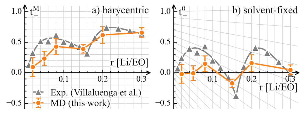
Figure 1: The transference number under a) barycentric RF and b) solvent-fixed RF in PEO-LiTFSI for different concentrations r [Li/EO] (the ratio of Li:ether oxygen). The conversion rule of $t_{+}^{\mathrm{}}$ as determined by Eq. 1 is shown by projecting the grid of a) to b). The experimental data and fitting of $t_{+}^{\mathrm{0}}$ re reproduced from Ref. 8. The transfer number in MD simulations are computed from the corresponding Onsager coefficients using Eq. 3, see the Supporting Information for simulation details.

While the two transference numbers are equivalent at the limit of infinite dilution ($\omega_{0}\to 1$), they become distinctly different at higher concentration. As shown in Fig. 1, at the concentration where negative $t_{+}^{\mathrm{0}}$ is observed, $t_{+}^{\mathrm{M}}$ is still positive. Moreover, $t_{+}^{\mathrm{}}$ generally shifts downward in the solvent-fixed RF as the concentration increases, as seen in Fig. 1. This trend can be expected, since at the other limit ($\omega_{0}\to 0$), $t_{+}^{\mathrm{M}}$ must converge to the $\omega_{-}$ in order to satisfy Eq. 1. This suggests that $t_{+}^{\mathrm{0}}$ will become increasingly sensitive at higher concentration since its value will be determined by the motion of a small fraction of solvent molecules.

The distinction between $t_{+}^{\mathrm{M}}$ and $t_{+}^{\mathrm{0}}$ may already explain why negative transference number is seldom observed in MD simulations, where the barycentric RF is the default setting. But more importantly, the strong dependency of $t_{+}^{\mathrm{}}$ on the RF suggests that the intuitive explanation of the observed negative $t_{+}^{\mathrm{0}}$ being due to the population of ion aggregates is not necessarily the case. Instead, as pointed out in recent studies^{15, 16, 17, 18, 19}, the explicit consideration of ion-ion correlations is essential to understand ion transport in polymer electrolytes.

In the following, we will show how the ion-ion correlations contribute to the negative transference number in light of the RF. In the Onsager phenomenological equations ²⁰, the flux $\mathbf{J}_{i}^{\mathrm{S}}$ of species under a reference frame $\mathrm{S}$ can be considered as the linear response of the external driving forces $\mathbf{X}_{j}^{\mathrm{}}$ acting on any species $j$:

$$\mathbf{J}_{i}^{\mathrm{S}}=\sum_{j}\Omega_{ij}^{\mathrm{S}}\mathbf{X}_{j}^{\mathrm{}}$$ (2)

where $\Omega_{ij}^{\mathrm{S}}$ are the Onsager coefficients. For the index $j$, here we denote the solvent as $0$, the cation as $+$, and the anion as $-$. In addition, the fluxes satisfy the following RF condition $\sum_{i}a_{i}^{\mathrm{S}}\mathbf{J}_{i}^{\mathrm{S}}=0$, where $a_{i}^{\mathrm{S}}$ are the proper weighing factors, i.e. $a_{i}^{\mathrm{M}}=M_{i}$ for the barycentric RF and $a_{i}^{\mathrm{0}}=\delta_{i0}$ for the solvent-fixed RF. Then, a unique set of the Onsager coefficients can be determined by applying the Onsager reciprocal relation: $\Omega_{ij}^{\mathrm{S}}=\Omega_{ji}^{\mathrm{S}}$, and the RF constraint $\sum_{i}a_{i}^{S}\Omega_{ij}^{\mathrm{S}}=0\ \forall j$.

Knowing these Onsager coefficients, one can express the transport properties of interest here, i.e. the transference number and the ionic conductivity, as:

$$t_{i}^{\mathrm{S}} =\frac{\sum_{j}q_{i}q_{j}\Omega_{ij}^{\mathrm{S}}}{\sum_{j,k}q_{j}q_{k}\Omega_{jk}^{\mathrm{S}}}$$ (3)

$$\sigma =\sum_{i,j}q_{i}q_{j}N_{\mathrm{A}}^{2}\Omega_{ij}^{\mathrm{S}}$$ (4)

where $q_{i}$ is the formal charge of $i$ and $N_{\mathrm{A}}$ is the Avogadro constant. It is worth noting that unlike the transference number, the ionic conductivity is RF-independent because of the charge neutrality condition.

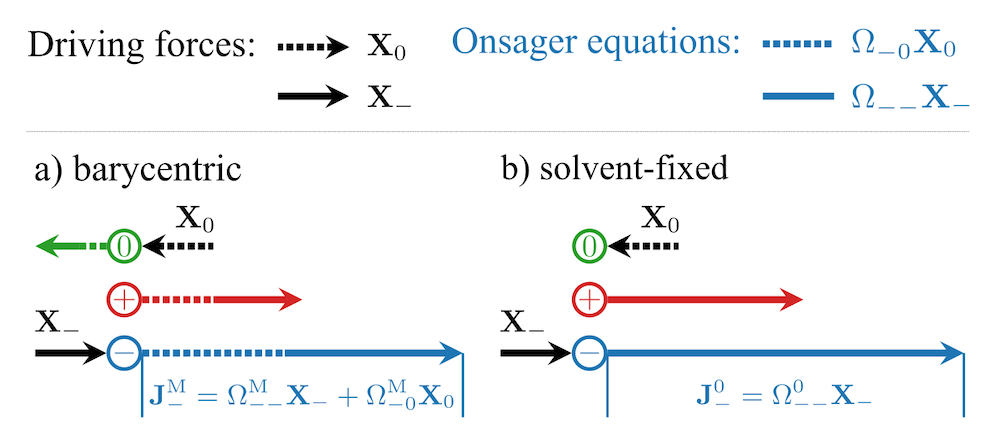
Figure 2: An illustration of the transformation procedure when converting $\Omega_{ij}^{\mathrm{M}}$ to $\Omega_{ij}^{\mathrm{0}}$ for the case where the driving force acting on cation is zero. The dashed lines indicate relevant parts related to the solvent.

While the transformation of $t_{+}^{\mathrm{}}$ from the solvent-fixed RF to the barycentric RF can follow the straightforward rule of Eq. 1, the corresponding RF transformation of $\Omega_{ij}^{\mathrm{}}$ is not trivial. This is illustrated by a simplified example shown in Fig 2, where driving force acting on the cation is assumed to be zero. In the barycentric RF both driving forces $\mathbf{X}_{0}^{\mathrm{}}$ acting on solvent and $\mathbf{X}_{-}^{\mathrm{}}$ acting on anion will contribute to the anion flux $\mathbf{J}_{-}^{\mathrm{M}}$. When transforming the Onsager coefficients to the solvent-fixed RF, only the driving force $\mathbf{X}_{-}^{\mathrm{}}$ contributes to the anion flux $\mathbf{J}_{-}^{\mathrm{0}}$, as $\Omega_{-0}^{\mathrm{0}}=0$ by construction.

Nevertheless, the general transformation rule can be derived using the independent fluxes and driving forces ²¹, which is consistent with the above constructions. Following the notation of Miller ²², one can consider only the $n-1$ independent fluxes and driving forces in a $n$ component system, where the flux of the solvent $\mathbf{J}_{0}^{\mathrm{}}$ is treated as a redundant variable. This leads to the following set of rules for the RF transformation:

$$A_{ij}^{\mathrm{RS}} =\delta_{ij}+\frac{c_{i}}{\sum_{k}a_{k}^{\mathrm{R}}c_{k}}\left(\frac{a_{0}^{\mathrm{R}}a_{j}^{\mathrm{S}}}{a_{0}^{\mathrm{S}}}-a_{j}^{\mathrm{R}}\right)$$ (5)

$$\mathbf{J}_{i}^{\mathrm{R}} =\sum_{j\neq 0}A_{ij}^{\mathrm{RS}}\mathbf{J}_{j}^{\mathrm{S}}$$ (6)

$$\Omega_{ij}^{\mathrm{R}} =\sum_{k,l\neq 0}A_{ik}^{\mathrm{RS}}\Omega_{kl}^{\mathrm{S}}A_{jl}^{\mathrm{RS}}$$ (7)

where $A_{ij}^{\mathrm{RS}}$ is the matrix that converts the independent fluxes from the reference frame S to R and $c_{i}$ is the molar concentration of species $i$. The coefficients $\Omega_{i0}^{\mathrm{R}}$ may then be fixed according to the RF constraint. The specific transformation equations for the barycentric and solvent-fixed RFs are provided in the Supporting Information.

This transformation provides the connection between $\Omega_{ij}^{\mathrm{0}}$ measured experimentally and $\Omega_{ij}^{\mathrm{M}}$ derived from MD simulations. Thus, one can compare Onsager coefficients under a common RF to see whether the simulation describes the same transport mechanism as in experiment or not. Here we computed Onsager coefficients following Miller’s derivation ⁶, with experimental measurements by Villaluenga et al. ⁸ MD simulations were performed using GROMACS ²³ and the General AMBER Force Field²⁴, from which Onsager coefficients were derived with an in-house analysis software. Details of the conversion and simulation procedure can be found in the Supporting Information. In addition, we shall note here that an alternative set of transport coefficients, i.e. the Maxwell-Stefan diffusion coefficients, were orginally reported from experiment ⁸, and they are consistent with the present framework (see the Supporting Information for the inter-conversion). However, the Onsager coefficients are favoured here because they are well-behaved at any given concentration and therefore helpful to understand the RF dependency of the ion-ion correlations.

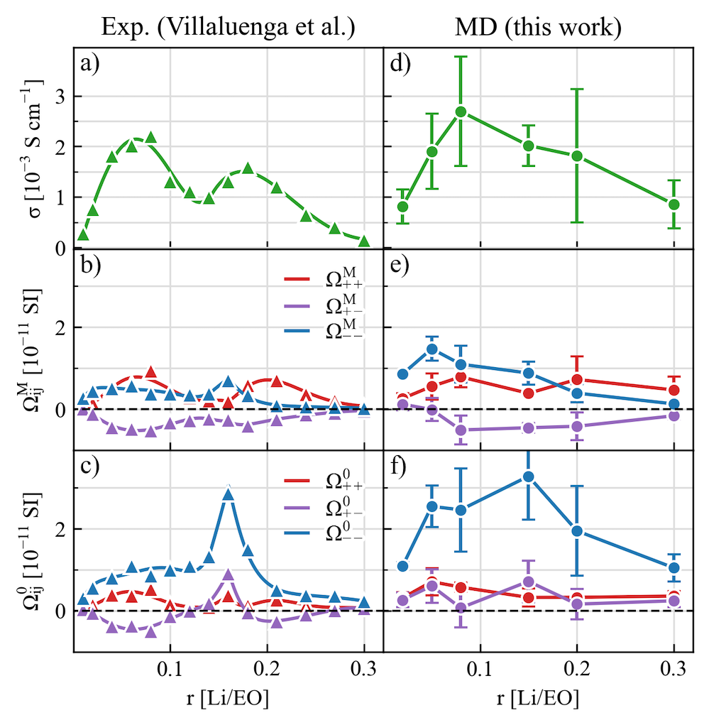
Figure 3: Ionic conductivity and Onsager coefficients under the barycentric and solvent-fixed derived from a-c) experimental measurements and d-f) MD simulations. The experimental measurements (triangle dots) and fittings (curved lines) are taken from Ref. 8. The MD simulation results are computed by fitting the mean displacement correlations functions, as detailed in the Supporting Information.

As shown in Fig. 3, the conductivity and Onsager coefficients obtained from MD simulations generally matches the experimental values. In particular, $\Omega_{+-}^{\mathrm{M}}$ is negative in the entire concentration range and this indicates an anti-correlation between cations and anions. Furthermore, we see that the experimentally observed negative transference number at $r=0.15$ is reproduced in the MD simulation, with consistent features of $\Omega_{ij}^{\mathrm{}}$, namely, $\Omega_{--}^{\mathrm{0}}>\Omega_{+-}^{\mathrm{0}}>\Omega_{++}^{\mathrm{0}}>0$ and $\Omega_{--}^{\mathrm{M}}>\Omega_{++}^{\mathrm{M}}>0>\Omega_{+-}^{\mathrm{M}}$. These results demonstrate that the experimentally observed negative transference number in PEO-LiTFSI systems is captured with the present force field parameterization used in the MD simulations.

If looking at the effects of RF, we see that $\Omega_{--}^{\mathrm{}}$ and $\Omega_{+-}^{\mathrm{}}$ changes more significantly upon RF transformation, as compared to $\Omega_{++}^{\mathrm{}}$. Especially, at $r=0.15$, $\Omega_{+-}^{\mathrm{M}}$ is negative while $\Omega_{+-}^{\mathrm{0}}$ is positive. This means that the driving force applied to the cations correlates to a co-directional anion flux in the solvent-fixed RF, but that an opposite anion flux is found in the barycentric RF. This, together with the observations made above, cannot be explained by any distribution of ideal charge carrying clusters.

To better understand the underlying physical account, we can look into the Onsager coefficients from a microscopic point of view, as they are related to the correlations functions of the fluxes. From the equations shown below, it is clear that the RF transformation is equivalent to transforming either the current-correlation function shown in Eq. 8 or, equivalently, the displacements of ions shown in Eq. 9. Thus, this result (Eq. 10) is consistent with Eq. 7, and Wheeler and Newman’s expression for $\Omega_{ij}^{\mathrm{0}}$ ²⁵.

$$\Omega_{ij}^{\mathrm{0}}= \frac{\beta}{3}\int d\mathbf{r}\int_{0}^{\infty}dt\left\langle\mathbf{J}_{i}^{\mathrm{0}}(0,0)\cdot\mathbf{J}_{j}^{\mathrm{0}}(\mathbf{r},t))\right\rangle$$ (8)

$$= \lim_{t\to\infty}\frac{\beta}{6VN_{\mathrm{A}}^{2}t}\left\langle\Delta\mathbf{r}_{i}^{\mathrm{0}}(t)\cdot\Delta\mathbf{r}_{j}^{\mathrm{0}}(t)\right\rangle$$ (9)

$$= \lim_{t\to\infty}\frac{\beta}{6VN_{\mathrm{A}}^{2}t}\left\langle\left(\sum_{k}A_{ik}^{\mathrm{0M}}\Delta\mathbf{r}_{k}^{\mathrm{M}}(t)\right)\cdot\left(\sum_{l}A_{jl}^{\mathrm{0M}}\Delta\mathbf{r}_{l}^{\mathrm{M}}(t)\right)\right\rangle$$ (10)

where $\beta=1/(k_{\mathrm{B}}T)$ is the inverse temperature, $N_{\mathrm{A}}$ is the Avogadro constant and $\Delta\mathbf{r}_{i}^{\mathrm{R}}(t)$ is the total displacement of species $i$ over a time interval $t$.

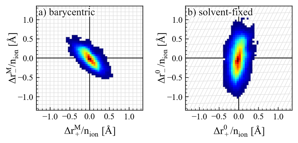
Figure 4: Transformation of the normalized displacement correlations upon a change of reference frame. $\Delta r^{\mathrm{M}}/n_{\mathrm{ion}}$ is the total displacement $\Delta r^{\mathrm{M}}$ (of cations “+" or anions “-”) normalized by the number of ions $n_{\mathrm{ion}}$. The correlation is obtained from a 400 ns MD trajectory, where the correlation between mean displacements of cations and anions over $\Delta t$=10ns is plotted in a) the barycentric RF and b) the solvent-fixed RF. The RF transformation according to Eq. 7 is visualized as the projection of grid lines from a) to b).

Based on this result, the conversion of Onsager coefficients upon an RF transformation can be visualized as an affine transformation of ion displacement, as shown in Fig. 4. At $r=0.15$, the displacement of cations and anions are apparently anti-correlated in the barycentric RF, while the correlation becomes positive in the solvent-fixed RF. This can be rationalized, since the motion of anions in the barycentric RF entails the motion of solvent in the opposite direction, giving rise to the enhanced anion motion and the positive cation-anion correlation in the solvent-fixed RF. On the other hand, the motion of cations induces a much less significant effect, as signified by the small distortion along the x-axis. This points in the direction that anions play a significant role for the transference number of Li⁺, not only by its relative motion to the cation.

Indeed, the sign of the experimentally measured $t_{+}^{\mathrm{0}}$ depends not only on $\Omega_{++}^{\mathrm{M}}-\Omega_{+-}^{\mathrm{M}}$, as is evident in Eq. 3, but also on the $\Omega_{--}^{\mathrm{M}}$ and the anion mass fraction. The importance of the anion-anion correlation and the anion mass is demonstrated in Fig. 5, where the partial derivative of $t_{0}^{\mathrm{+}}$ shows its strong dependency on the anion mass and Onsager coefficients. An increase of the anion mass introduces an even stronger reduction of the transference number $t_{0}^{\mathrm{+}}$, and therefore $t_{0}^{\mathrm{+}}$ is more likely to be negative. The same effect occurs when the anion-anion correlation becomes stronger and $\Omega_{--}^{\mathrm{M}}$ becomes larger. This suggests a direct connection between the observed negative $t_{+}^{\mathrm{0}}$ and a strong anion-anion correlation found at higher concentrations. The latter effect was also indicated in a recent X-ray scattering study of PEO-LiTFSI systems ¹².

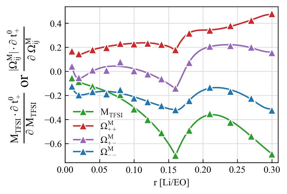
Figure 5: The sensitivity of transference number $t_{+}^{\mathrm{0}}$ in solvent-fixed RF to the variations in the anion molecular weight $\mathrm{M}_{\ch{TFSI}}$ and different Onsager coefficients $\Omega_{ij}^{\mathrm{M}}$ in the barycentric RF. The analysis is done by evaluating the partial derivative of $t_{+}^{\mathrm{0}}$ to the logarithm of $\mathrm{M}_{\ch{TFSI}}$ or $|\Omega_{ij}^{\mathrm{M}}|$, with data derived from experimental measurements in Ref. 8. Note that $\Omega_{+-}^{\mathrm{M}}$ is mostly negative as shown in Fig. 3, while the other variables are positive.

In summary, our present analysis reveals a strong RF dependency of the transference number and the Onsager coefficients in the PEO-LiTFSI system. With a proper transformation, the Onsager coefficients can be used as a rigorous test to compare the transport properties from experimental measurements and MD simulations, as shown here. This will provide a new ground to refine force field parameterization, for example, by including the subtle effects of electronic polarization ²⁶, although we found that the standard force field already captures the main features observed in experiments.

Not only do our results demonstrate that the experimentally observed negative $t_{+}^{\mathrm{0}}$ can be reproduced with MD simulations, but they also show that cations and anions are anti-correlated in the barycentric RF ($\Omega_{+-}^{\mathrm{M}}$<0) throughout the entire concentration range in both experiment and simulation. While this does not rule out the possibility of short-lived ion aggregates, neither does it support a transport mechanism based on negatively-charged ion clusters. Instead, we show that a large anion mass and strong anion-anion correlations can be responsible for a negative transference number of $t_{+}^{\mathrm{0}}$.

Furthermore, the RF-dependence of ion-ion correlations suggests that any discussions about ion-ion correlations need to be done within the same RF. This may shed light on why a different observation was made regarding the sign of $t_{+}^{\mathrm{}}$ with alternative experimental approaches such as electrophoretic NMR (eNMR) ¹⁰.

Although we do not expect that all discrepancies in transport properties between different experimental approaches and between experiment and simulation can be resolved by the present analysis, insights regarding the RF dependency of ion-ion correlations, and direct comparison of the complete set of Onsager coefficients between experiment and simulation as demonstrated in this work would be essential to elucidate the ion transport mechanism in polymer electrolytes and alike concentrated electrolyte systems.

This work has been supported by the European Research Council (ERC), grant no. 771777 “FUN POLYSTORE” and the Swedish Research Council (VR), grant no. 2019-05012. The authors thanks funding from the Swedish National Strategic e-Science program eSSENCE, STandUP for Energy and BASE (Batteries Sweden). The simulations were performed on the resources provided by the Swedish National Infrastructure for Computing (SNIC) at PDC.

Details of MD simulations and force field parameters; Computation and conversion of Onsager coefficients in different RFs; Conversion between different sets of transport equations; List of symbols.

References

- Mindemark et al. 2018 Mindemark, J.; Lacey, M. J.; Bowden, T.; Brandell, D. Beyond PEO—Alternative host materials for Li+-conducting solid polymer electrolytes. Prog. Polym. Sci. 2018, 81, 114–143
- Choo et al. 2020 Choo, Y.; Halat, D. M.; Villaluenga, I.; Timachova, K.; Balsara, N. P. Diffusion and migration in polymer electrolytes. Prog. Polym. Sci. 2020, 103, 101220
- Evans et al. 1987 Evans, J.; Vincent, C. A.; Bruce, P. G. Electrochemical measurement of transference numbers in polymer electrolytes. Polymer 1987, 28, 2324–2328
- Bruce and Vincent 1987 Bruce, P. G.; Vincent, C. A. Steady state current flow in solid binary electrolyte cells. J. Electroanal. Chem. Interfacial Electrochem. 1987, 225, 1–17
- Newman and Balsara 2020 Newman, J.; Balsara, N. P. Electrochemical Systems; Wiley, 2020
- Miller 1966 Miller, D. G. Application of Irreversible Thermodynamics to Electrolyte Solutions. I. Determination of Ionic Transport Coefficients for Isothermal Vector Transport Processes in Binary Electrolyte Systems. J. Phys. Chem. 1966, 70, 2639–2659
- Zwanzig 1965 Zwanzig, R. Time-Correlation Functions and Transport Coefficients in Statistical Mechanics. Annu. Rev. Phys. Chem. 1965, 16, 67–102
- Villaluenga et al. 2018 Villaluenga, I.; Pesko, D. M.; Timachova, K.; Feng, Z.; Newman, J.; Srinivasan, V.; Balsara, N. P. Negative Stefan-Maxwell Diffusion Coefficients and Complete Electrochemical Transport Characterization of Homopolymer and Block Copolymer Electrolytes. J. Electrochem. Soc. 2018, 165, A2766–A2773
- Hoffman et al. 2021 Hoffman, Z. J.; Shah, D. B.; Balsara, N. P. Temperature and concentration dependence of the ionic transport properties of poly(ethylene oxide) electrolytes. Solid State Ion. 2021, 370, 115751
- Rosenwinkel and Schönhoff 2019 Rosenwinkel, M. P.; Schönhoff, M. Lithium Transference Numbers in PEO/LiTFSA Electrolytes Determined by Electrophoretic NMR. J. Electrochem. Soc. 2019, 166, A1977–A1983
- Molinari et al. 2018 Molinari, N.; Mailoa, J. P.; Kozinsky, B. Effect of Salt Concentration on Ion Clustering and Transport in Polymer Solid Electrolytes: A Molecular Dynamics Study of PEO–LiTFSI. Chem. Mater. 2018, 30, 6298–6306
- Loo et al. 2021 Loo, W. S.; Fang, C.; Balsara, N. P.; Wang, R. Uncovering Local Correlations in Polymer Electrolytes by X-ray Scattering and Molecular Dynamics Simulations. Macromolecules 2021, 54, 6639–6648
- France-Lanord and Grossman 2019 France-Lanord, A.; Grossman, J. C. Correlations from Ion Pairing and the Nernst-Einstein Equation. Phys. Rev. Lett. 2019, 122, 136001
- Woolf and Harris 1978 Woolf, L. A.; Harris, K. R. Velocity correlation coefficients as an expression of particle–particle interactions in (electrolyte) solutions. J. Chem. Soc., Faraday Trans. 1 1978, 74, 933–947
- Vargas-Barbosa and Roling 2020 Vargas-Barbosa, N. M.; Roling, B. Dynamic Ion Correlations in Solid and Liquid Electrolytes: How Do They Affect Charge and Mass Transport? ChemElectroChem 2020, 7, 367–385
- Zhang et al. 2020 Zhang, Z.; Wheatle, B. K.; Krajniak, J.; Keith, J. R.; Ganesan, V. Ion Mobilities, Transference Numbers, and Inverse Haven Ratios of Polymeric Ionic Liquids. ACS Macro Lett. 2020, 9, 84–89
- Pfeifer et al. 2021 Pfeifer, S.; Ackermann, F.; Sälzer, F.; Schönhoff, M.; Roling, B. Quantification of cation–cation, anion–anion and cation–anion correlations in Li salt/glyme mixtures by combining very-low-frequency impedance spectroscopy with diffusion and electrophoretic NMR. Phys. Chem. Chem. Phys. 2021, 23, 628–640
- Fong et al. 2021 Fong, K. D.; Self, J.; McCloskey, B. D.; Persson, K. A. Ion Correlations and Their Impact on Transport in Polymer-Based Electrolytes. Macromolecules 2021, 54, 2575–2591
- Gudla et al. 2021 Gudla, H.; Shao, Y.; Phunnarungsi, S.; Brandell, D.; Zhang, C. Importance of the Ion-Pair Lifetime in Polymer Electrolytes. J. Phys. Chem. Lett. 2021, 12, 8460–8464
- Onsager 1945 Onsager, L. Theories and problems of liquid diffusion. Ann. N. Y. Acad. Sci. 1945, 46, 241–265
- Kirkwood et al. 1960 Kirkwood, J. G.; Baldwin, R. L.; Dunlop, P. J.; Gosting, L. J.; Kegeles, G. Flow Equations and Frames of Reference for Isothermal Diffusion in Liquids. J. Chem. Phys. 1960, 33, 1505–1513
- Miller 1986 Miller, D. G. Some comments on multicomponent diffusion: negative main term diffusion coefficients, second law constraints, solvent choices, and reference frame transformations. J. Phys. Chem. 1986, 90, 1509–1519
- Abraham et al. 2015 Abraham, M. J.; Murtola, T.; Schulz, R.; Páll, S.; Smith, J. C.; Hess, B.; Lindahl, E. GROMACS: High performance molecular simulations through multi-level parallelism from laptops to supercomputers. SoftwareX 2015, 1-2, 19–25
- Wang et al. 2004 Wang, J.; Wolf, R. M.; Caldwell, J. W.; Kollman, P. A.; Case, D. A. Development and testing of a general amber force field. J. Comput. Chem. 2004, 25, 1157–1174
- Wheeler and Newman 2004 Wheeler, D. R.; Newman, J. Molecular Dynamics Simulations of Multicomponent Diffusion. 1. Equilibrium Method. J. Phys. Chem. B 2004, 108, 18353–18361
- Borodin 2009 Borodin, O. Polarizable Force Field Development and Molecular Dynamics Simulations of Ionic Liquids. J. Phys. Chem. B 2009, 113, 11463–11478