Deformable Radar Polygon: A Lightweight and Predictable Occupancy Representation for Short-range Collision Avoidance

Abstract

Inferring the drivable area in a scene is a key capability for ensuring the vehicle avoids obstacles and enabling safe autonomous driving. However, a traditional occupancy grid map suffers from high memory consumption when forming a fine-resolution grid for a large map. In this paper, we propose a lightweight, accurate, and predictable occupancy representation for automotive radars working for short-range applications that take interest in instantaneous free space surrounding the sensor. This new occupancy format is a polygon composed of a bunch of vertices selected from noisy radar measurements, which covers free space inside and gives a Doppler moving velocity for each vertex. It not only takes a very small memory and computing resources for storage and updating at every timeslot but also has the predictable shape-change property based on vertex’s Doppler velocity. We name this kind of occupancy representation “deformable radar polygon”. Two formation algorithms for radar polygon are introduced for both single timeslot and continuous inverse sensor model update. To fit this new polygon representation, a matrix-form collision detection method has been modeled as well. The radar polygon algorithms and collision detection model have been validated via extensive experiments with real collected data and simulations, showing that the deformable radar polygon is very competitive in terms of its completeness, smoothness, accuracy, lightweight as well as the shape-predictable property. Our codes will be made available at https://github.com/Xiangyu-Gao/deformable_radar_polygon_occupancy_representation.

I Introduction

Occupancy mapping is an important component in road scene understanding for autonomous driving. It encapsulates information about the drivable area or free space, road obstacles and enables safe autonomous driving. A good occupancy representation should have a pixel value of 1 when corresponding location is occupied by obstacles, and a pixel value of 0 when free space. For a lot of short-range applications, e.g., vehicle back-off planning, the instantaneous free space surrounding the sensor is required [1, 2], instead of a whole-view map. Motivated by this, we focus on finding an accurate and also lightweight occupancy representation for instantaneous free space estimation.

A lot of algorithms have been proposed to deeply investigate occupancy mapping and free space detection. Traditionally, occupancy grid mapping is performed by applying Bayesian filtering and using hand-crafted inverse sensor model (ISM) functions [3, 4, 5, 6, 7, 8, 9, 10, 11, 12]. However, the main drawback of occupancy grid map is the high memory consumption when forming a fine-resolution grid for a large map. In our case, even if we are only interested in the instantaneous free space for each timeslot, a complete large map is required for occupancy grid updating to keep the consistency of confidence scores across multiple timeslots. Even with fast efficient computing methods in prior works [13, 14], it has not been fully addressed.

To solve this problem, we propose a lightweight solution for the occupancy representation of automotive radars, called deformable radar polygon. Specifically, based on the dense points provided by radar and the fact that short-range applications usually care more about the closest surrounding obstacles, we select vertices from the point clouds surrounding radar and connect all vertices to form a polygon that covers all free space. In this way, instead of storing and updating the whole map and its pixel value, we now only need to store a group of vertices and their confidence, which is much more convenient. Similar to the binary meaning in occupancy grid representation, the region within the polygon is assumed as the safety region (i.e., equivalent to having a pixel value of 0), and the region outside of the polygon is assumed to be occupied or dangerous. To form the radar polygon, we proposed two ways: one is by deterministic selecting vertices for each time-slot independently which will be introduced in Section III-B, the other one is more continuous by applying modified ISM in polygon update which will be introduced in Section III-C. Results in Section VII-A show that the radar polygon method consumes low storing memory, runs fast, keeps high smoothness, and forms complete and accurate occupancy representation with comparable performance to gird.

To detect potential collision that lies outside of the polygon region, we model a collision detection algorithm in Section V with the odd-even principle [15] and a matrix-form function, which is much more efficient than the way of checking the stored map and its pixel value table for grid map.

One exciting thing for radar polygon is that the vertices selected from radar points are with a Doppler velocity for each since automotive radars can measure and estimate the Doppler velocities of detected targets. The Doppler velocity can depict the movement of vertex (shrink or expansion) along the radial direction, which makes it possible to predict the shape of future radar polygon and feed the predicted results to downstream applications, e.g., route planning, and collision avoidance, for providing additional information.

In summary, the main contributions of this paper are three-fold:

• A new polygon-based occupancy representation that has the advantages of completeness, smoothness, accuracy, lightweight as well as shape-predictable property.

• Two formation algorithms for radar polygon that work for a single timeslot and continuous ISM update. Extensive experiments for validating the algorithms.

• A matrix-form collision detection algorithm that works for polygon representation.

II Related Work

For LiDAR occupancy grid generation [9], a delta function ISM is typically used, while it is more common to see a Gaussian variant (in range and azimuth) of the delta function ISM when generating radar occupancy grid since radar data is sparser and noisier. In [10, 12], the Gaussian ISM was upgraded to rate detection probability by calculating the plausibility of range, angle, and amplitude for each measurement. In [3], ISM works with ego-motion velocity-dependent parameters by giving higher values for the uncertainty ellipses when there is higher ego-velocity leading to less detection. In addition, [5] proposed a special ISM that converts the measurement signal-to-noise ratio (SNR) to the probability of detection using the Swerling-1 model. To fit the needs of more and more complicated application scenarios, radar occupancy methods have been extended to numerically efficient mapping in three dimensions [14, 5]. Without using hand-crafted ISM, the recent deep-learning methods have been used in occupancy grid mapping to improve accuracy via end-to-end model [8, 9, 6] and classification [7].

Based on the generated radar occupancy grid, plenty of downstream applications have been explored, e,g., free space detection using image analysis and dynamic b-spline contour tracking [16], detection of parallel-parked vehicles and cross-parked vehicles [17], and detection of available parking space [18], etc. Beyond occupancy mapping, vehicle perception using radars is attracting more interest in the community due to the availability of radars on off-the-shelf cars, the comparatively low price, 3D/4D estimation capability [1, 2], and robustness under harsh weather [19]. Novel applications, e.g., super-resolution imaging [2], road object detection [20] are proposed to take full advantage of automotive radars.

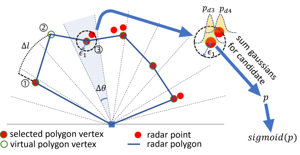
Figure 1: Procedures of forming a radar polygon. After sampling the FoV with $\Delta\theta$, a vertex (point 3) is selected based on normalized evidence probability or a virtual one (point 2) is created for each sampling sector.

III Radar Polygon for Occupancy Representation

III-A Problem Formulation

For a list of radar detections $\mathbf{E}$ where each detection $e$ includes the measurement of 3 dimensions $x$, $y$, $z$, Doppler velocity $v$ and SNR, we are looking to select subset points $\mathbf{E}^{\prime}$ from it as the vertices and construct an occupancy polygon that maximizes available free space, minimizes the number of selected points, and reduces the interference of false alarms. This is indeed an NP-hard Knapsack problem, and to solve it approximately we propose the below heuristic solution.

III-B Radar Polygon Formation for Single Time-slot

We first introduce a deterministic algorithm for forming radar polygon for each timeslot without any recursion or accumulation from previous timeslots. Since we are interested in the occupancy status in 2D bird-eye-view (BEV), the preparation step for point clouds with additional dimensions would be to project them into the 2D plane. For example, for $z$ dim. we select all points with reasonable height (i.e., greater than $-1.5\text{\,}\mathrm{m}$ and less than $3\text{\,}\mathrm{m}$) and project them to the 2D $x$-$y$ plane by compressing the height.

To determine the polygon vertex for different azimuth directions, we sample the whole field of view (FoV) with fixed angle interval $\Delta\theta$ (see Fig. 1). For each sampling sector, we define below policies to select a vertex or create a virtual one.

• We find the closest point as a candidate, and its neighboring points within distance $\epsilon_{1}$. Each point will be given its detection probability $p_{d}$ calculated from SNR [5] using Swerling-1 model Eq. (1).

  $$p_{d}^{\text{Swerling}}(\text{SNR})=p_{\textnormal{fa}}^{\frac{1}{1+\text{SNR}}}$$ (1)

  where $p_{\textnormal{fa}}$ is the false alarm rate used in point cloud extraction. The spatial occupancy evidence for each point is given by a Gaussian distribution $p_{d}\cdot\mathcal{N}(\bm{\mu},\,\bm{\Sigma})$ [4], where $\bm{\mu}$ is point location and $\bm{\Sigma}$ is a fixed parameter. Since $99.7\%$ of the energy of normal distribution is constrained in $3$-sigma region, we choose $\bm{\Sigma}=\bm{I}(\epsilon_{1}/3)^{2}$. We will sum up the occupancy evidence of all points on the location of candidate point and scale it with sigmoid normalization Eq. (2), and if the resulted value $\tilde{p}$ is greater than threshold $p_{\textnormal{thr}}$, we assume the candidate is the vertex, otherwise, we will look for the second-closest point and continue above operations. Note that $\epsilon_{1}$ limits the number of points we need to consider or compute, which relieves computation load.

  $$\tilde{p}=\textit{sigmoid}(p)=\frac{1}{2}+\frac{1}{2}\left[1+\exp\left(\frac{-\left(p-\bar{p}\right)}{\sigma_{p}}\right)\right]^{-1}$$ (2)

  where $\bar{p},\,\sigma_{p}$ is the shift and scaling factor.

• If there is no point in the sampling sector satisfies the above rules, we will check if to make a virtual vertex located at the boundary here (e.g., point 2 in Fig. 1) with zero Doppler velocity and SNR. The checking process is to measure the cross-range length $\Delta l$ (Arc length) between any two adjacent non-virtual vertices (e.g., point 1 and 2) and if it is smaller than the predefined threshold $l_{\textnormal{thr}}$ we will remove the virtual vertices between them. We bring in this checking process to avoid forming small spikes.

At last, all vertices plus the origin point are connected in sequence to form the radar polygon.

III-C Radar Polygon Update with Inverse Sensor Model

The single timeslot algorithm outputs the up-to-date occupancy polygon surrounding the ego-vehicle where the inside region is free space and the outside is occupied. To utilize the history measurements to get a higher-confidence polygon boundary and fill in the out-of-view gap on two sides of the ego-vehicle, we consider updating the radar polygon using the inverse sensor model (ISM). With the assumption that the vertex in one sampling sector across multiple timeslots can be tracked and belongs to the same target, ISM can be employed to calculate a posterior probability or confidence score using previous data. Note that when applying ISM to traditional grids, the cell is fixed, while in our case the vertex is moving, which works only when the above assumption is satisfied.

Mathematically, the problem is defined as: given the polygon vertices set $E^{\prime}_{t-1}$ and vertices confidence set $L_{t-1}$ for time $t-1$, and the noisy radar measurements $E_{t}$ and vehicle pose $Z_{t}$ for time $t$, the proposed radar polygon update algorithm gives the new polygon with $E^{\prime}_{t}$ and $L_{t}$ for current time $t$. To solve this, we first update $E^{\prime}_{t-1}$ with $Z_{t}$ for its latest location at $t$ and incorporate the updated $E^{\prime}_{t-1}$ into $E_{t}$. Assuming the vehicle pose $Z_{t}$ includes $(x_{t},y_{t},\phi_{t})$, the global position along $x,y$ and orientation $\phi$. Projecting $E^{\prime}_{t-1}$ to latest car coordinate at $t$ is done by compensating car motion $(x_{t}-x_{t-1},y_{t}-y_{t-1})$ and orientation change $\phi_{t}-\phi_{t-1}$.^†

For each sampling sector, a vertex candidate $e^{\prime}_{t}$ is selected from $E_{t}$ according to Section III-B, which is then dealt with in the following cases:

A old vertex: This means the candidate vertex $e^{\prime}_{t}$ is from the set $E^{\prime}_{t-1}$. If its confidence $\ell_{t-1}$ is negative, we would give up it and go back to find a new candidate. Otherwise, we give it a confidence penalty $-l_{\text{pen}}$ and add it to set $E^{\prime}_{t}$.

Trackable to old vertex: This means vertex $e^{\prime}_{t}$ is not from $E^{\prime}_{t-1}$ and is close to the latest location of the previous vertex $e^{\prime}_{t-1}$ for the same sampling sector within threshold $\epsilon_{2}$. If it satisfies, the following ISM Eq. (3) would be used to update its posterior probability $\ell_{t}$ based on the Bayes’ theorem [12].

$$\ell_{t}(e_{t}^{\prime})=\ell_{t-1}(e_{t-1}^{\prime})+\log\frac{\tilde{p}\left(e_{t}^{\prime}\mid E_{t},Z_{t}\right)}{1-\tilde{p}\left(e_{t}^{\prime}\mid E_{t},Z_{t}\right)}-\ell_{o}$$ (3)

where $\tilde{p}\left(e_{t}^{\prime}\mid E_{t},Z_{t}\right)$ is the normalized occupancy evidence of $e_{t}^{\prime}$ from Eq. (2), and $E_{t},Z_{t}$ are put here to describe the current measurement or vehicle pose. The initial confidence $\ell_{o}$ is typically assumed as 0, since nothing is known about the surrounding environment before the first measurement.

Uncertain emerging vertex: if $e^{\prime}_{t}$ is not old and not trackable to old vertex, we consider it might be an emerging vertex. All the emerging vertices are considered uncertain at first and are stored in set $U$, to reduce false alarms. When the vertex in $U$ has been associated with new-coming vertices more than one time, it would be moved from $U$ to the polygon set. The association happens when the inter-distance is smaller than $\epsilon_{2}$.

Missing: This is for the case of no candidate vertex being found in a sampling sector, a virtual vertex with 0 confidence is added to $E^{\prime}_{t}$ following the algorithm in Section III-B.

The pseudo code of ISM-based polygon update algorithm is shown in Algorithm 1.

Algorithm 1 Radar Polygon Formation and Update with ISM

1:procedure Polygon_ISM($E_{t},Z_{t},L_{t-1},E^{\prime}_{t-1},U$)

2:     if $t=1$ then

3:         form initial polygon $E_{1}^{\prime}$, following Section III-B

4:     else

5:         update $E^{\prime}_{t-1}$ with $Z_{t}$, do $E_{t}\leftarrow E_{t}\cup E^{\prime}_{t-1}$

6:         for each sampling set $S_{t}$ in $E_{t}$ do

7:              find the closet candidate vertex $e^{\prime}_{t}$ from $S_{t}$

8:              if not exist $e^{\prime}_{t}$ then

9:                  create a virtual vertex with confidence 0

10:                  continue               

11:              if $\left(e^{\prime}_{t}\textbf{ in }E^{\prime}_{t-1}\textbf{ and }\ell_{t-1}(e^{\prime}_{t})<0\right)$ or its spatial occupancy evidence $\tilde{p}$ $<p_{\text{thr}}$ then

12:                  remove $e^{\prime}_{t}$ from $S_{t}$

13:                  goto line 7, refind candidate               

14:              if $e^{\prime}_{t}$ in $E^{\prime}_{t-1}$ then

15:                  $\ell_{t}(e^{\prime}_{t})\leftarrow\ell_{t}(e^{\prime}_{t})-\ell_{\textnormal{pen}}$

16:              else if $e^{\prime}_{t}$ tracked to previous vertex $e^{\prime}_{t-1}$ then

17:                  $\ell_{t}(e^{\prime}_{t})\leftarrow\ell_{t-1}(e^{\prime}_{t-1})+\log\frac{\tilde{p}}{1-\tilde{p}}-\ell_{o}$

18:              else

19:                  if $e_{t}^{\prime}$ trackable among $U$ and age $>$ 1 then

20:                       $\ell_{t}(e_{t}^{\prime})\leftarrow\log\frac{\tilde{p}}{1-\tilde{p}}-\ell_{o}$

21:                       add $e^{\prime}_{t}$ to $E^{\prime}_{t}$ and add $l_{t}$ to $L_{t}$

22:                  else

23:                       add $e_{t}^{\prime}$ to $U$ and update $U$                   

24:                  continue               

25:              add $e^{\prime}_{t}$ to $E^{\prime}_{t}$ and add $l_{t}$ to $L_{t}$               

26:     output $E_{t}^{\prime}$, $L_{t},U$ $\triangleright$ Ending

Remark: The radar data collected from real-world radars usually contains noisy measurements/clutter due to the unwanted echoes returned from the ground, atmosphere, etc. Our proposed algorithms deal with it in two ways. First, the vertices with small SNRs or few nearby measurements are filtered out due to the low detection probability. Second, the ISM-based polygon update provides a extra correction overtime via consideing the tracking consistency and emerging uncertainty of vertices.

IV Deformable Radar Polygon

IV-A Deformable Polygon Prediction

The vertices that constitute the radar polygon have Doppler velocities, which can describe their instant movement along the radial direction (i.e., the direction from vertex to radar). By assuming the radial velocity of a vertex is constant within a short period and ignoring its tangential velocity (rotation), we can estimate the vertex’s future location by calculating and adding its radial movement using the current Doppler velocity (see Fig. 2(a)). That is, for a vertex with location $(x,y)$ and Doppler velocity $\mathbf{v}=(v_{\textnormal{x}},v_{\textnormal{y}})$, its radial movement $(\Delta x,\Delta y)$ for radar sensor $(x_{\textnormal{s}},y_{\textnormal{s}})$ within duration $\Delta t$ is given by:

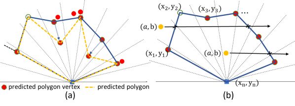
Figure 2: (a) Example of a deformable radar polygon. (b) Illustration of checking collision detection.

$$(\Delta x,\Delta y)=(v_{\textnormal{x}},v_{\textnormal{y}})\times\Delta t$$ (4)

$$(v_{\textnormal{x}},v_{\textnormal{y}})=\frac{(x-x_{\textnormal{s}},\ y-y_{\textnormal{s}})}{\sqrt{(x-x_{\textnormal{s}})^{2}+(y-y_{\textnormal{s}})^{2}}}\times v$$

Adding the estimated radial movement to current vertex, we can predict its new location $(x^{\prime},y^{\prime})=(x,y)+(\Delta x,\Delta y)$. The virtual vertex has zero Doppler velocity such that its location is unchanged. After predicting the new location of all vertices of the current polygon and connecting them in sequence, we will form the predicted polygon for $\Delta t$ time later. Since the polygon shape change can be roughly and manually predicted based on Doppler velocity, we call this kind of radar polygon “deformable polygon”.

 

$$\mathbf{F}(a,b)=\begin{bmatrix}y_{1}-y_{2}&x_{2}-x_{1}\\ y_{2}-y_{3}&x_{3}-x_{2}\\ \vdots&\vdots\\ y_{n-1}-y_{n}&x_{n}-x_{n-1}\\ y_{n}-y_{1}&x_{1}-x_{n}\\ \end{bmatrix}_{n\times 2}\begin{bmatrix}a\\ b\end{bmatrix}+\begin{bmatrix}x_{1}(y_{2}-y_{1})-y_{1}(x_{2}-x_{1})\\ x_{2}(y_{3}-y_{2})-y_{2}(x_{3}-x_{2})\\ \vdots\\ x_{n-1}(y_{n}-y_{n-1})-y_{n-1}(x_{n}-x_{n-1})\\ x_{n}(y_{1}-y_{n})-y_{n}(x_{1}-x_{n})\\ \end{bmatrix}_{n\times 1}$$ (5)

$$\mathbf{F}(a,b)=\mathbf{P}[\mathbf{Y_{n}}\;-\mathbf{X_{n}}]\begin{bmatrix}a\\ b\end{bmatrix}-(\mathbf{PY_{n}})\circ\mathbf{X_{n}}+(\mathbf{PX_{n}})\circ\mathbf{Y_{n}}$$ (6)

where $\mathbf{P}=\begin{bmatrix}1&-1&0&\ldots&0&0\\ 0&1&-1&\ldots&0&0\\ \vdots&\vdots&\vdots&\ddots&\vdots&\vdots\\ 0&0&0&\ldots&1&-1\\ -1&0&0&\ldots&0&1\\ \end{bmatrix}_{n\times n}$ and $\circ$ is the Hadamard product (element-wise multiplication).

IV-B Alternative to Pose Information for ISM

The ISM requires the accurate pose information of the vehicle for projecting the radar measurements from different time-slots to the same coordinate. In our case, Eq. (3) describes the usage of vehicle pose $Z_{t}=(x_{t}.y_{t},\phi_{t})$ in projecting the old radar polygon $E^{\prime}_{t-1}$ to the global coordinate of time $t$ and get the up-to-date polygon. Since the deformable polygon prediction property, i.e., the future shape of radar polygon can be roughly predicted with Doppler velocity, it is potential to use this deformation prediction to replace the required pose information under some critical cases when the localization sensors (e.g., inertial measurement unit, global positioning system) are not available and no large lateral movement exists. Detailedly, the cross-time compensating^† for vehicle motion $(x_{t}-x_{t-1},y_{t}-y_{t-1})$ and orientation change $\phi_{t}-\phi_{t-1}$ in Section III-C can be roughly replaced by moving the vertex by $\mathbf{v}_{t-1}\Delta t$ where $\mathbf{v}_{t-1}$ is the corresponding Doppler velocity of vertex and $\Delta t$ is the slot duration. Note that Doppler velocity measures the relative moving speed along radial direction, so even for static objects, there would be non-zero Doppler velocities reflecting the relative movement when the car moves.

V Collision Detection for Radar Polygon

The collision detection for polygon-based occupancy representation is modeled in this section. Assume the polygon has $n$ vertices $(x_{1},y_{1}),\ (x_{2},y_{2}),\dots,(x_{n},y_{n})$ sorted in azimuth ascending order, there is a point $(a,b)$ that needs to be checked if it has any collision to the region outside of the polygon. This problem is equivalent to asking whether point $(a,b)$ in the plane lies inside, or outside of the polygon.

One simple way of solving it is the even–odd rule algorithm [15]. For details, we draw a horizontal line to the right of point $(a,b)$ and extend it to infinity and count the number of times the line intersects with polygon edges (assuming the polygon boundary is not strictly horizontal). If the line intersects the edge an even number of times, $(a,b)$ is on the outside of the polygon; If an odd number of times, $(a,b)$ is on the inside of the polygon (see Fig. 2(b) for example).

Mathematically, the condition when horizontal line starting from point $(a,b)$ (to its right) intersects edge $(x_{1},y_{1})\rightarrow(x_{2},y_{2})$ can be expressed as:

$$\begin{gathered}\frac{(b-y_{1})(x_{2}-x_{1})}{y_{2}-y_{1}}>a-x_{1},\ \min(y_{1},y_{2})<b<\max(y_{1},y_{2})\end{gathered}$$

To check the intersection between horizontal line and all edges make up the polygon, we let $\mathbf{X_{n}}=[x_{1},\ x_{2},\dots,x_{n}]^{\intercal}$, $\mathbf{Y_{n}}=[y_{1},\ y_{2},\dots,y_{n}]^{\intercal}$, and define a matrix function $\mathbf{F}$ shown in Eq. (6) as below with its full expansion in Eq. (5).

For point $(a,b)$, function $\mathbf{F}(a,b)$ will return a column vector that needs to be made element-wise multiplication with $\mathbf{PY_{n}}$ and $\mathbf{Q}$, (i.e., $\mathbf{F}(a,b)\circ\mathbf{PY_{n}}\circ\mathbf{Q}$) to count the number of elements less than zero, where $\mathbf{P}$ and $\mathbf{Q}$ are defined in Eq. (6) (7) respectively. If it is odd number, $(a,b)$ is on the inside of polygon and if it is even number or zero, $(a,b)$ is on the outside of polygon and there exists a collision.

$$\mathbf{Q}=\begin{bmatrix}q_{1},q_{2},\dots,q_{n}\end{bmatrix}\quad\text{where}$$ (7)

$$q_{i}=\begin{cases}1,&\text{if }\min(y_{i},y_{i+1})<b<\max(y_{i},y_{i+1})\\ 0,&\text{otherwise}\end{cases}$$

The collision detection function (6) can be extended from a point to a input matrix. Let input be $\mathbf{A}=\begin{bmatrix}a_{1},a_{2},\ldots,a_{m}\\ b_{1},b_{2},\ldots,b_{m}\\ \end{bmatrix}$, the new detection function $\mathbf{F}(\mathbf{A})$ is given by Eq. (8). For each column of result $\mathbf{F}(\mathbf{A})$, we can apply above checking process for collision detection.

$$\mathbf{F}(\mathbf{A})=\mathbf{P}\begin{bmatrix}\mathbf{Y_{n}},\mathbf{-X_{n}}\end{bmatrix}\mathbf{A}-(\mathbf{PY_{n}})\circ\mathbf{X_{n}}+(\mathbf{PX_{n}})\circ\mathbf{Y_{n}}$$ (8)

Significantly, using the deformable polygon property, we can even make the collision detection for a short time later. This is done by first predicting the new polygon shape $\mathbf{X^{\prime}_{n}},\mathbf{Y^{\prime}_{n}}$ based on current polygon shape $\mathbf{X_{n}},\mathbf{Y_{n}}$ and Doppler velocity components projected onto $x$, $y$ direction $\mathbf{V_{xn}},\mathbf{V_{yn}}$ using Eq. (9). Then new polygon shape $\mathbf{X^{\prime}_{n}},\mathbf{Y^{\prime}_{n}}$ is input to Eq. (6) (8) for collision detection.

$$\begin{bmatrix}\mathbf{X^{\prime}_{n}},\mathbf{Y^{\prime}_{n}}\end{bmatrix}=\begin{bmatrix}\mathbf{X_{n}},\mathbf{Y_{n}}\end{bmatrix}+\begin{bmatrix}\mathbf{V_{xn}},\mathbf{V_{yn}}\end{bmatrix}$$ (9)

VI Implementation

VI-A Testbed Setup

The testbed shown in Fig. 3 includes 4 radars two of them are mounted on the front side of the car and two are on the rear side. All radars are placed with a certain shift on boresight to increase the overall FoV (light green region). The radars are configured with maximum detectable range $20\text{\,}\mathrm{m}$, range resolution $4.3\text{\,}\mathrm{c}\mathrm{m}$, azimuth FoV $\pm$$$, elevation FoV $\pm$$$, Doppler resolution $0.22\text{\,}\mathrm{m}\mathrm{/}\mathrm{s}$, Doppler ambiguity $7.1\text{\,}\mathrm{m}\mathrm{/}\mathrm{s}$, and frame rate $10\text{\,}\mathrm{f}\mathrm{p}\mathrm{s}$. The test car is also equipped with cameras for synchronized data collection, relying on the closest timestamp match.

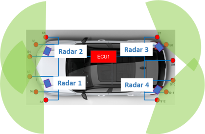
Figure 3: Testbed with 4 radars (blue rectangles). The FoV of radars are visualized with the light green color.

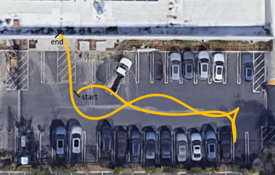
Figure 4: BEV parking lot where the car backing-off experiment was performed along the yellow trajectory. Image is from Google map.

VI-B Experiments

Experiments were performed at the parking lot with the scenario of the classic car backing off and the pedestrian/car passing by. The point clouds of 4 radars were recorded along with the camera images and their own timestamps. The vehicle pose and trajectory required by ISM were obtained from odometry [2, 21] calculation. The ground truth for evaluating occupancy status was generated by human labeling on camera BEV images and projecting the label to radar coordinates via the BEV-radar sensor calibration and transformation. The hyper-parameters used in radar polygon formation and ISM were chosen by grid search. Specifically, $\epsilon_{1}=1,\,\epsilon_{2}=1,\,l_{\textnormal{thr}}=$7.5\text{\,}\mathrm{m}$,\,\bar{p}=12.1,\,\sigma_{p}=7.132,\,p_{\textnormal{thr}}=0.62,\ell_{\textnormal{pen}}=0.5$. Other system parameters includes sampling angle $\Delta\theta=2\degree$, CFAR false alarm rate $p_{\textnormal{fa}}=10^{-3}$. For ease of computing, we formed a polygon for two front radars and the other one for two rear radars, and made the union of two polygons as final result. All experiments were run on a laptop with $2.9\text{\,}\mathrm{G}\mathrm{H}\mathrm{z}$ 6-Core Intel i9 processor and $32\text{\,}\mathrm{G}\mathrm{B}$ of RAM to have a fair comparison between different algorithms.

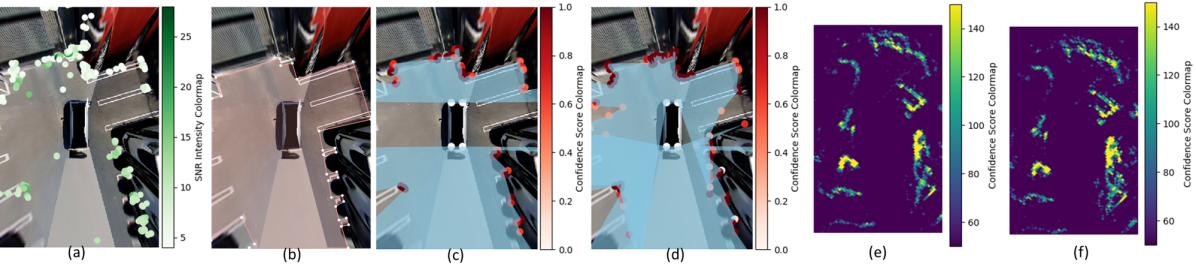
Figure 5: Examples in self-collected dataset: (a) point cloud visualization, (b) free space ground truth (in red), (c) single-shot radar polygon result (free space is in blue), (d) ISM-based radar polygon result, (e)-(f) occupancy grid results from [10] and [12].

VII Evaluation

VII-A Numerical Evaluation

A numerical evaluation was performed on the car backing-off experiment by analyzing the accuracy and smoothness of proposed radar polygon approaches and comparing them with state-of-art occupancy grid works [10, 12]. The experiment data was recorded at the parking lot shown in Fig. 4 with the vehicle trajectory highlighted with yellow curves. We implemented the proposed radar polygon (single frame), radar polygon with ISM method, and the occupancy grip mapping methods Werber et al. [10], Li et al. [12] with the collected data. For [10, 12], we consider a grid map of $$60\text{\,}\mathrm{m}$\times$60\text{\,}\mathrm{m}$$ with $0.3\text{\,}\mathrm{m}$ resolution for the accumulation of every $70$ frames.

We presented one snapshot of the recorded data along with its point cloud visualization, free space ground truth, and the output from different methods in Fig. 5(a)-(f). From the comparison, we see that the radar polygon is accurate and complete as it depicts the clear contours of the surrounding parked cars and the empty parking space sandwiched between two parked cars. Besides, the radar polygon with ISM would fill in the out-of-view gap on two sides of the vehicle.

The numerical evaluation was done by calculating the intersection over union (IoU) between ground truth and radar polygon (IoU-gt) to show completeness, calculating the IoU between every two successive polygon predictions (IoU-smooth) to show smoothness, and calculating the mean square error (MSE) between ground truth and polygon/occupancy grid to show accuracy. The averaged results are presented in Table. LABEL:tab:nume_evl and the detailed IoU-gt, IoU-smooth results along vehicle motion is shown in Fig. 6. From those results, we learn that the radar polygon method achieves around $70\%$ IoU-gt and perfect $90\%$ IoU-smooth. With adopting the ISM in polygon formation, all metrics got significant improvement on both averaged (Table. LABEL:tab:nume_evl) and instantaneous results (Fig. 6). When comparing the radar polygons to the occupancy grids [10, 12], the IoU-based metric didn’t work anymore. Thus, we measured the MSE of free space predictions. Specifically, we assumed the inner region of the polygon is free and the grid cell with the confidence less than a threshold is free. Results in Table. LABEL:tab:nume_evl show that radar polygon with ISM has comparable MSE performance with referred occupancy grids at around $0.1$, showing adequate accuracy.

TABLE I: The evaluation results of algorithms in terms of IoU-gt, IoU-smooth, MSE, and running time.

Method	IoU-gt	IoU-smooth	MSE	Run time
radar polygon	66.21%	86.45%	0.2979	$20.10\text{\,}\mathrm{m}\mathrm{s}$
radar polygon (ISM)	73.12%	89.68%	0.1302	$19.75\text{\,}\mathrm{m}\mathrm{s}$
Werber et al. [10]	–	–	0.0897	$98.38\text{\,}\mathrm{m}\mathrm{s}$
Li et al. [12]	–	–	0.1151	$97.65\text{\,}\mathrm{m}\mathrm{s}$

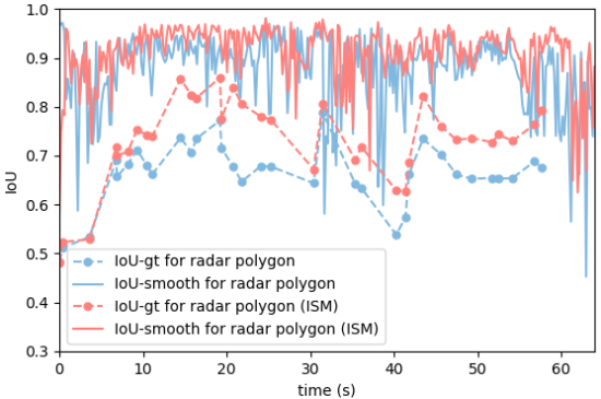
Figure 6: The instantaneous IoU-gt, IoU-smooth values for single-shot radar polygon (blue lines) and ISM-based radar polygon (red lines) across $60\text{\,}\mathrm{s}$.

VII-B Required Storing Memory Analysis

In addition to the advantages of completeness, smoothness, and accuracy, the radar polygon has a very lightweight storage memory consumption. As the vehicle moves and for each timeslot, only the vertex information (location, SNR, confidence) is needed to be stored and transferred to the next timeslot. The vertex size would not be continuously accumulated since the rules guarantee at most one vertex per sampling interval in both the formation and update stage. Therefore, the storing memory for radar polygon is approximate $\mathcal{O}(M)$ with the number of samplings $M$ for covering FoV. While for the occupancy grid, the storing memory is usually linearly increased with the number of cells in a gird, i.e., $\mathcal{O}(N^{2})$ with $N$ cells in each dimension. For example, a $$60\text{\,}\mathrm{m}$\times$60\text{\,}\mathrm{m}$$ grid map with $0.3\text{\,}\mathrm{m}$ resolution requires $N=200$. To get a similar resolution for radius of $30\text{\,}\mathrm{m}$, a radar polygon with $0.5\degree$ sampling interval requires $M=720$. Assume a vertex and a cell would occupy same-size memory space, then a rough calculation of the division between their overall storing memory is $\mathcal{O}(N^{2})/\mathcal{O}(M)=200^{2}/720\approx 56$, showing remarkable deduction on memory consumption with radar polygon.

VII-C Polygon Prediction

To show what the Doppler velocity on each vertex looks like in a radar polygon, more data were collected under two cases: pedestrians passing by, and vehicles passing by. We visualized the polygon results formed by rear radars in Fig. 7 and plotted measured Doppler velocities for polygon vertices using red arrows. From those results, we could tell that the polygon has a good representation of passing pedestrians and moving vehicles. The plotted Doppler velocity also indicates the moving speed and direction of the vertex, of which the effectiveness would be primarily verified next.

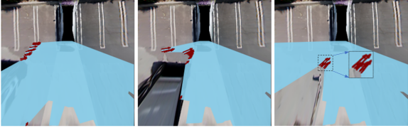
Figure 7: Rear-radar polygon results for moving vehicles and pedestrian. The Doppler velocity for each vertex is visualized with red arrow indicating the vertex motion in next timeslot.

To quantitatively evaluate how well the proposed polygon prediction performs (Section IV), we made the one-to-one comparison between the current-frame radar polygon and the predicted polygon from the last frame in Fig. 8, and calculated the IoU between them. Three examples are from car backing-off, pedestrian, and vehicle passing-by experiments, respectively. In Fig. 8, current-frame radar polygons are shown with a light-blue region, and predicted polygons are plotted with the dotted line. The predicted polygons are highly overlapped with the new measurements with IoU above $0.9$, which shows a good prediction performance and primitively verifies the correctness of our deformable radar polygon idea.

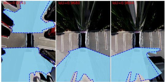
Figure 8: Polygon prediction results for car backing-off, pedestrian and vehicle passing-by experiments. Light blue region is the measured radar polygon while the dotted line forms the predicted radar polygon from last frame.

VII-D Impact of Sampling Angle $\Delta\theta$

Sampling angle $\Delta\theta$ is an important system parameter that affects the performance and required resources. A numerical evaluation was done for the single-shot radar polygon, and ISM-based radar polygon with varying $\Delta\theta$. As shown in Fig. 9, with smaller $\Delta\theta$, the formed radar polygon would be more complete and accurate, showing better IoU-gt and IoU-smooth for both methods. Overall, the accuracy, and smoothness decrease is not drastic with $\Delta\theta$ changing from $0.5\degree$ to $10\degree$. On the other hand, decreased sampling angle brings in computing complexity issues and storing memory issues since there would be more vertices to be calculated, stored and updated, and vice versa. Therefore, it is important to find a good trade-off point of $\Delta\theta$ fitting specific application requirements.

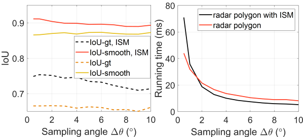
Figure 9: Impact of varying sampling angle $\Delta\theta$ on (a) accuracy and smoothness IoU-gt and IoU-smooth, and (b) running time for two radar polygon methods.

VII-E Generalization to Other Dataset

Besides the self-collected dataset, We evaluated the proposed algorithms on the open-source RadarScenes dataset [22], with the focus on the city-road driving case. Specifically, a clip of data for 916 frames were selected. Similar to the previous numerical evaluation, the IoU-gt, IoU-smooth, MSE metrics were calculated for 4 algorithms and were shown in Table LABEL:tab:nume_evl_radarscene. From it, we can tell that the radar polygon method only achieves around $40\%$ IoU-gt and $60\%$ IoU-smoothm, while the ISM-based method improve two metrics to $75.86\%$, $82.92\%$, respectively. The huge gain comes from that the history vertices fill the unknown gap and the uncertain vertex design reduces false alarms. The comparison to Werber et al. [10], Li et al. [12] shows the ISM-based radar polygon reaches the accuracy as good as the time and memory-consuming occupancy grid methods, with the MSE around $0.02$. We also presented one snapshot of the recorded data along with its output from four algorithms in Fig. 10(a)-(d).

The qualitative results of polygon prediction are presented in Fig. 11. Even in the sophisticated city-road driving case, the deformable polygon still brings off a good short-term prediction performance with a high overlapping with the new measurements. We also noticed that when new points/objects appear, the prediction performance usually degrades because of missing those.

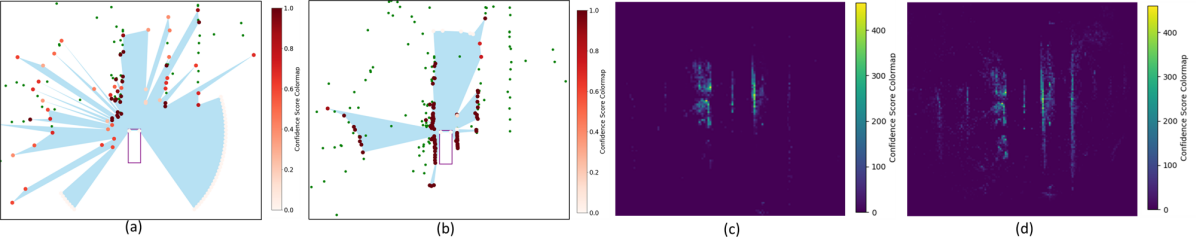
Figure 10: Examples in RadarScenes dataset: (a) single-shot radar polygon result (free space is in blue), (b) ISM-based radar polygon result, (c)-(d) occupancy grid results from [10] and [12].

TABLE II: The evaluation results of algorithms in terms of IoU-gt, IoU-smooth, MSE, and running time on RadarScenes.

Method	IoU-gt	IoU-smooth	MSE	Run time
radar polygon	39.59%	61.15%	0.0665	$6.61\text{\,}\mathrm{m}\mathrm{s}$
radar polygon (ISM)	75.86%	82.92%	0.0221	$11.03\text{\,}\mathrm{m}\mathrm{s}$
Werber et al. [10]	–	–	0.0194	$29.47\text{\,}\mathrm{m}\mathrm{s}$
Li et al. [12]	–	–	0.0319	$29.72\text{\,}\mathrm{m}\mathrm{s}$

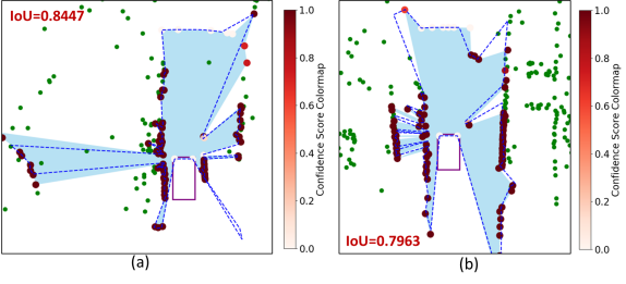
Figure 11: Polygon prediction results for RadarScenes dataset. Light blue region is the measured radar polygon while the dotted line forms the predicted radar polygon from last frame.

VIII Discussion

VIII-A Strength and Limitation

The radar polygon method is good at forming complete and accurate occupancy representation, keeping high smoothness, consuming low storing memory, and running fast. While for limitations, it only focuses on the instantaneous free space around the vehicle and ignores others behind obstructions, which may not fit for applications that request a whole-scene map. If the sampling FoV and distance are extremely large, the real contour of objects may be in the polygon free space. Besides, its performance under static (ego-car and object) scenario drops (see the first $5\text{\,}\mathrm{s}$ of Fig. 6) since the low SNR of point clouds and the false alarms resulted from less gain of Doppler estimation [1].

IX Conclusion

In this paper, we explained the proposed radar polygon formation algorithm using radar point cloud input. Besides, we modeled the collision detection method for fitting this new polygon representation. The radar polygon and collision detection model have been validated via extensive experiments with real collected data. It shows that the radar polygon is very competitive in terms of its simplicity, accuracy, and robustness. Besides, the deformable polygon idea was verified by showing the high IoU correlation between the predicted radar polygon and the actually generated one. For future work, we will explore the approaches to make the radar polygon fit long-range scenarios and be more robust.

References

- [1] X. Gao, G. Xing, S. Roy, and H. Liu, “Experiments with mmwave automotive radar test-bed,” in 2019 53rd Asilomar Conference on Signals, Systems, and Computers, 2019, pp. 1–6.
- [2] X. Gao, S. Roy, and G. Xing, “Mimo-sar: A hierarchical high-resolution imaging algorithm for mmwave fmcw radar in autonomous driving,” IEEE Transactions on Vehicular Technology, vol. 70, no. 8, pp. 7322–7334, 2021.
- [3] R. Prophet, H. Stark, M. Hoffmann, C. Sturm, and M. Vossiek, “Adaptions for automotive radar based occupancy gridmaps,” in 2018 IEEE MTT-S International Conference on Microwaves for Intelligent Mobility (ICMIM), 2018, pp. 1–4.
- [4] P. Berthold, M. Michaelis, T. Luettel, D. Meissner, and H.-J. Wuensche, “Deriving spatial occupancy evidence from radar detection data,” in 2020 IEEE Intelligent Vehicles Symposium (IV), 2020, pp. 831–836.
- [5] J. Degerman, T. Pernstål, and K. Alenljung, “3d occupancy grid mapping using statistical radar models,” in 2016 IEEE Intelligent Vehicles Symposium (IV), 2016, pp. 902–908.
- [6] F. E. Nowruzi, D. Kolhatkar, P. Kapoor, F. Al Hassanat, E. J. Heravi, R. Laganiere, J. Rebut, and W. Malik, “Deep open space segmentation using automotive radar,” in 2020 IEEE MTT-S International Conference on Microwaves for Intelligent Mobility (ICMIM), 2020, pp. 1–4.
- [7] J. Lombacher, K. Laudt, M. Hahn, J. Dickmann, and C. Wöhler, “Semantic radar grids,” in 2017 IEEE Intelligent Vehicles Symposium (IV), 2017, pp. 1170–1175.
- [8] N. Engelhardt, R. Pérez, and Q. Rao, “Occupancy grids generation using deep radar network for autonomous driving,” in 2019 IEEE Intelligent Transportation Systems Conference (ITSC), 2019, pp. 2866–2871.
- [9] L. Sless, B. E. Shlomo, G. Cohen, and S. Oron, “Road scene understanding by occupancy grid learning from sparse radar clusters using semantic segmentation,” in 2019 IEEE/CVF International Conference on Computer Vision Workshop (ICCVW), 2019, pp. 867–875.
- [10] K. Werber, M. Rapp, J. Klappstein, M. Hahn, J. Dickmann, K. Dietmayer, and C. Waldschmidt, “Automotive radar gridmap representations,” in 2015 IEEE MTT-S International Conference on Microwaves for Intelligent Mobility (ICMIM), 2015, pp. 1–4.
- [11] C. Diehl, E. Feicho, A. Schwambach, T. Dammeier, E. Mares, and T. Bertram, “Radar-based dynamic occupancy grid mapping and object detection,” in 2020 IEEE 23rd International Conference on Intelligent Transportation Systems (ITSC), 2020, pp. 1–6.
- [12] M. Li, Z. Feng, M. Stolz, M. Kunert, R. Henze, and F. Küçükay, “High resolution radar-based occupancy grid mapping and free space detection,” in VEHITS, 2018.
- [13] F. Homm, N. Kaempchen, J. Ota, and D. Burschka, “Efficient occupancy grid computation on the gpu with lidar and radar for road boundary detection,” in 2010 IEEE Intelligent Vehicles Symposium, 2010, pp. 1006–1013.
- [14] M. Slutsky and D. Dobkin, “Fast implementation of volumetric occupancy grids,” in 2019 IEEE Intelligent Vehicles Symposium (IV), 2019, pp. 750–755.
- [15] M. Shimrat, “Algorithm 112: Position of point relative to polygon,” Commun. ACM, vol. 5, no. 8, p. 434, Aug. 1962. [Online]. Available: https://doi.org/10.1145/368637.368653
- [16] M. Schreier and V. Willert, “Robust free space detection in occupancy grid maps by methods of image analysis and dynamic b-spline contour tracking,” in 2012 15th International IEEE Conference on Intelligent Transportation Systems, 2012, pp. 514–521.
- [17] R. Dubé, M. Hahn, M. Schütz, J. Dickmann, and D. Gingras, “Detection of parked vehicles from a radar based occupancy grid,” in 2014 IEEE Intelligent Vehicles Symposium Proceedings, 2014, pp. 1415–1420.
- [18] R. Prophet, M. Hoffmann, M. Vossiek, G. Li, and C. Sturm, “Parking space detection from a radar based target list,” in 2017 IEEE MTT-S International Conference on Microwaves for Intelligent Mobility (ICMIM), 2017, pp. 91–94.
- [19] X. Gao, S. Roy, G. Xing, and S. Jin, “Perception through 2d-mimo fmcw automotive radar under adverse weather,” in 2021 IEEE International Conference on Autonomous Systems (ICAS), 2021, pp. 1–5.
- [20] X. Gao, G. Xing, S. Roy, and H. Liu, “Ramp-cnn: A novel neural network for enhanced automotive radar object recognition,” IEEE Sensors Journal, vol. 21, no. 4, pp. 5119–5132, 2021.
- [21] D. Kellner, M. Barjenbruch, J. Klappstein, J. Dickmann, and K. Dietmayer, “Instantaneous ego-motion estimation using multiple doppler radars,” in 2014 IEEE International Conference on Robotics and Automation (ICRA), 2014, pp. 1592–1597.
- [22] O. Schumann, M. Hahn, N. Scheiner, F. Weishaupt, J. Tilly, J. Dickmann, and C. Wöhler, “RadarScenes: A Real-World Radar Point Cloud Data Set for Automotive Applications,” Mar. 2021. [Online]. Available: https://doi.org/10.5281/zenodo.4559821